
Submitted:
04 September 2025
Posted:
08 September 2025
You are already at the latest version
Abstract
The influence of a material sensor in the component’s surface layer on its fatigue strength is investigated by FE simulation. A material model for metastable austenite transformation to martensite from literature is adapted to include effects significant to this scenario. Sensor operation is simulated for single overloads and load cycles and a fatigue assessment is carried out. The detrimental effect on component life stems from the neutralization of the mean compressive stress from shot peening by sensor manufacture and a notch effect during sensor triggering. A straightforward approach for incorporating the effect of the material sensor into component design with worst-case assumptions is presented. The adverse effect can be averted or minimized by appropriate positioning of the sensor.
Keywords:
material sensor
; metastable austenite
; sensor-integrating machine element
; material model
1. Introduction
The load-induced transformation of metastable austenite to martensite, primarily found in stainless steels like 1.4301 (AISI 304/X5CrNi18-10), can be used for sensing applications. A concept for sensor-integrating machine elements is explored, where austenite content is adjusted locally in an initially martensitic surface layer by laser heat treatment of a component, and eddy current sensors are applied on the locally austenitised surface (Figure 1, [1]) for capturing martensite content evolution as a measure of the loads it experienced.
When accumulating plastic strain, metastable austenite transforms to martensite. Therefore, martensite content can be interpreted as a measure of the loads the component has experienced. As this microstructural transformation takes place without the need for electrical power and can be read out by eddy current testing with eddy current sensors at large intervals, it is well suited for ultra-low power applications where electrical power for data processing is e. g. generated via energy harvesting. Austenite and martensite phases can be differentiated by eddy current probing due to their different electromagnetic properties.
As the material sensor affects component stress – as will be explored in this paper – it should not be placed in the most highly loaded spot. Nonetheless, it needs to be placed in a relatively highly loaded location in order to be stressed above its triggering threshold.
In this paper, the influence of the sensor placement on the component is investigated. Starting with a shot peened surface with martensite saturation, austenite is generated locally by laser heat treatment. A microsection of such a sensor spot is shown in Figure 2. The volume differential between the two phases leads to high residual stresses, which affect component life due to the mean stress effect. Furthermore, austenite has a much lower yield strength than martensite; the sensor spot thus yields when the rest of the component is stressed elastically. Plastic straining is in fact necessary for the microstrutural transformation to take place, and thus for the sensor to function. When the sensor spot flows plastically, it has a reduced apparent stiffness, and acts as a notch to the component it is embedded in. With rising martensite content, the yield strength differential as well as the volume differential decreases; the effect on component fatigue thus changes over time.
The quantification of a derating factor containing both stress concentration as well as the mean stress effect is pursued numerically via a material model capable of portraying martensite content evolution inside a finite element model. A simulation-based approach is chosen, as the stress distribution underneath the material sensor cannot easily be recorded by measurement, and this approach leads to the largest qualitative insight.
2. Material Model
A material model by Gallée et al. is implemented, which is capable of simulating martensite evolution of the yielding material [2]. Martensite and austenite are modeled as two separate phases and overall behavior is calculated via a phase mixture law by Pilvin [3], which is based on the work of Berveiller and Zaoui [4]. Martensite develops according to a model by Shin [5], which depends on accumulated plastic strain in the austenite phase, modified by Gallée [6] for additionally including the dependence of austenite transformation on hydrostatic stress. The individual phases harden isotropically following Voce law [7] and kinematically according to Armstrong-Frederick [8] with an additional Prager type component [9]. The model includes a transformation plasticity effect modeled as proposed by Leblond [10], which leads to additional deviatoric strains due to the phase evolution. While the model would be capable of representing viscoplasticity, only quasistatic loading, i. e. a low loading frequency is simulated in this paper for the sake of simplicity. For a detailed description of the model, see [2].
Unlike in the original version developed for orthotropic sheet metal, yielding according to Hill’s criterion for anisotropic materials is not implemented, but the von Mises yield criterion for isotropic materials is used instead for the laser heat treated spot. Further modifications to this model are made concerning hydrostatic volume change and model constants.
2.1. Volume Change
The original model only contains deviatoric transformation plasticity as an additional strain due to phase change, but does not describe the hydrostatic volume change between the two phases. As the sensor is situated at the component’s surface, it experiences no stresses orthogonal to the surface. Hydrostatic volume change therefore does not lead to fully hydrostatic stresses, which would not influence the sensor’s yielding behavior. Strains due to volume change are modeled analogous to thermal strains as follows:
with the length difference between austenite and martensite in each direction % [11], the martensite volume fraction , the difference in martensite volume fraction compared to the initial state, and the identity tensor . The strain applies to the phase mixture, i. e. it is applied like a strain due to external loading.
In order to model the stress state due to the volume differential between the sensor and the surface layer, the sensor is gradually generated in the FE model based on the real-world manufacturing process by starting from martensite saturation in the surface layer, and then pulling the martensite volume fraction down in the sensor volume by a prescribed amount over many small time steps. As the material starts to yield during this process due to the resulting high tensile stresses caused by the laterally constrained contraction, a fraction of the prescribed martensite reduction in each step is not realized when the sensor slightly transforms back to higher martensite content. This simulation artefact leads to the simulation not starting at exactly 100% austenite (cf. Figure 14), yet close enough for practical purposes. Without the use of a detailed thermal model of the laser heat treatment, this manual adjustment of the martensite content leads to a worst case analysis.
2.2. Model Constant Fit
As Gallée developed the material model primarily for forming applications, i. e. one load cycle, the material constant fit is unsatisfying for a high number of load cycles. With Gallée’s constants, material behavior is strongly dependent on isotropic hardening; by hardening, the austenite phase yield limit can increase by 1532 , which unrealistically lies above the ultimate strength. This means that after a few load cycles, no more yielding of the austenite phase, and thus no more martensite content evolution takes place.
Due to this limitation new material constants are fitted for 1.4301 to experiments with more load cycles. The availability of fatigue data from these experiments is an additional benefit; otherwise material data from two vastly different research projects would need to be mixed.
Medhurst [12] performed fatigue tests for sensory utilizable stainless steels with different amounts of prestrain. He recorded martensite content and yield limits for different amounts of prestrain as well as stress-strain diagrams for inital loading. Thus, martensite content after simulated prestraining and the yield limit at reloading after prestraining can be fitted. Additionally, the stress amplitude evolution in low-cycle fatigue (LCF) testing allows for material constant fitting over many load cycles, although martensite content was not measured over time. As Medhurst [12] worked with cold rolled sheet metal, specimens with zero austenite content are unfortunately not available. The use of the material model constants below 25% martensite content is therefore an unvalidated extrapolation. Furthermore, the principal direction properties of sheet metal are transferred to be omnidirectional.
In Table 1 material constants used in the following analysis are compared with Gallée’s paper. The comparison is grouped by equation or rather physical context. For further unchanged constants used in additional equations with no alterations, see [2]. The qualitative change is marked in the last column. Isotropic hardening is completely reversed; going from modeling intense cyclic hardening to mild cyclic softening. Cyclic hardening now stems primarily from the increased martensite transformation rate. Further changes are comparatively small (marked as ≈). The phase of initial cyclic softening followed by continuous cyclic hardening where non-metastable steels would exhibit a horizontal curve progression can be observed in Figure 3 where experimental and simulated results for a LCF experiment are compared. Results from simulated prestraining are shown in Table 2.
3. FE Model
Computations are carried out in FE program Code Aster [13] with the material model implemented as a UMAT (user material subroutine). The most basic configuration of a sensor spot on a cuboid under uniaxial tension is investigated. This geometry can be analyzed exploiting quarter symmetry. The configuration is shown in Figure 4.
3.1. Sensor Geometry
Sensor geometry is gauged off a microsection of a lasered sensor spot (Figure 2). As the transition between austenite and martensite in the surface layer is quite abrupt, it is represented as an interface in the FE model. The sensor spot has a depth of approx. 120 and a curvature of . The surface martensite layer has about the same depth as the sensor spot. The core is a phase mixture of approx. 65% martensite saturation for sufficient core strength in the exemplifying splined shaft application. The radius at the corner of the sensor spot, surface layer, and base material is modeled with a radius of .
3.2. Simulation Stability
The interface between the yielding and due to phase transformation contracting sensor spot and the surface layer presents a discontinuity that leads to a phenomenon known as spurious oscillations or checkerboarding where the stresses near the interface oscillate between positive and negative values from element to element. Initially this leads to wrong results; at higher loading the solver fails.
As attempts to model a less abrupt interface with a gradual change in martensite content over a few elements were unsuccessful, this issue is remedied by the extended finite element method (XFEM) [14,15,16]. Near the interface a mesh of standard elements is “enriched” with basis functions incorporating Heaviside step functions. XFEM’s ability to model discontinuities not conforming to the mesh – which is particularly useful for growing cracks – is not used here and instead the XFEM interface follows a manually cut face in a structured mesh (Figure 5). This is necessary to overcome issues with the FE program’s XFEM implementation which when cutting through elements with XFEM in some cases assigns initial martensite content by interpolating from both sides of the interface, leading to destabilizing spikes of drastically different stiffness properties on one side of the interface.
As the method by default models openable cracks and simply bonded contacts are not implemented for XFEM, a cohesively bonded contact with an unreachably large rupture load is applied in the FE program.
3.3. Cycle Jumping
Due to the transient characteristics of the sensor, behavior over the entire fatigue life needs to be worked out. However, it would be unfeasible to explicitly simulate the high number of load cycles occuring during fatigue loading. Following some highly non-linear evolution during initial loading, it is possible to approximate behavior by piece-wise linearizations. A cycle jumping technique introduced in [17] is therefore used for speeding up the computation. The internal variables of the material model at the start of the next load cycle are extrapolated from the results of the last five explicitly calculated load cycles.
A permissible jumping step size is determined with an error approximation method [18] based on Richardson extrapolation. The jumping procedure is run from the same starting point for four cycle jumps with the current step size and for two cycle jumps with double the step size and one cycle jump with quadruple the step size. Maximum stress is compared for the end points of the three parallel analyses. Step size is then doubled, when the local convergence error is less than %. Conversely, a halving of the step size is implemented, should the error rise again, although this option was not needed.
3.4. Load
The simulated cuboid (Figure 4) cut out of a larger structural component is operated with prescribed strains on its sides for uniaxial tension. Applicable displacements are calculated for a prescribed nominal stress of this cuboid.
Residual stresses from shot peening are not applied in the FE model in order to provide greater contrast concerning sensor-caused phenomena in the following figures. Initial residual stress is comparatively insignificant to the sensor, as it strains by multiples of the commonly used % yield limit during manufacturing. As the martensitic surface layer exhibits linear elastic behavior throughout all analyses, the stress amplitude does not depend on residual stress and for mean stress effects in fatigue assessments, residual stress can be linearly superposed.
4. Fatigue Assessment
The influence of time-dependent stress amplitudes on component fatigue can be assessed in a computation of non-linear damage accumulation. The calculation process known as “FKM non-linear” [19] is used with damage parameter . Resultant loads of each FEM node are rainflow counted; damage accumulation is calculated with stress and strain from FEM. Component failure is expected at 100% damage. Material fatigue data are taken from Medhurst [12] for 1.4301.
Fatigue data for maximally pre-strained specimens, i. e. specimens with martensite saturation, are used for assessing the surface layer. Fatigue data for non pre-strained specimens, i. e. specimens with low martensite content, can be used for assessing the sensor for single-amplitude loading. The “low” martensite content being 25% presents a source of error that can only be quantified by fatigue experiments that lie outside the scope of the current research programme.
The sensor is essentially operated strain controlled with approximately constant strain for constant stress amplitude of the base component, as it has negligible influence on macroscopic component deformation. This type of loading is equivalent to strain controlled constant amplitude fatigue testing. Fatigue assessment for variable amplitude loading would not be permissible for the sensor, as the fatigue material data do not capture transient effects. Variable amplitude loading assessment would be permissible for the surface layer, as it does not exhibit transient behavior due to martensite saturation.
5. FE Analysis
All following FE result figures are zoomed in to a cube’s edge length of 1 for sake of clarity.
5.1. Initial State
Figure 6 shows the residual stress after simulated “heat treatment” as described in Section 2.1. The sensor is pre-stressed to about 130% ; the base material at the sensor’s edge is at a considerable tensile stress of about 70% . Compressive residual stresses from shot peening are neutralized.
5.2. Single Load Cycle (overload detection)
Figure 7a,b show the stress state when a single load cycle with an amplitude of 125% is applied starting from the initial state. The critical spot in the base component as well as the sensor is at the sensor’s edge tangential to the loading direction (on the left edge in these figures).
Figure 7c,d show the system at an amplitude below yield stress (25% ). No derating factor needs to be calculated for loads well below the sensor yield strength, as the tolerable load cycle number lies orders of magnitude above VHCF load cycle numbers.
Figure 8 shows stress factors that relate local stresses to nominal stress for different overloads. For high overloads, the stress factor inside the sensor lies below one due to it yielding with weak hardening effects. Higher overloads lead to higher stress factors in the surface layer.
5.3. Muliple Cycles (Load Logger)
The model was run for 1.2 × 10⁴ load cycles at 125% . As a load logger, the sensor should be placed on a component with an equal expected life – in this case one with a maximum stress of approx. 440 .
Figure 9, Figure 10 and Figure 11 show the martensite content, residual stress and stress amplitude at three characteristic stages. As can be seen from Figure 9b, sensor transformation is quite homogenous.
Note that Figure 10 and Figure 11 use different scales than Figure 6 and Figure 7 in order to better highlight the minute differences. Figure 11 does not start at zero for the same reason.
Compared to Figure 7 the location of maximum stress has moved to the edge of the martensite layer underneath the sensor after cyclic softening. Calculations in this location are imprecise, as the phase fraction and geometry of this transition region are vague approximations of Figure 2. The results can be evaluated nonetheless, as the stress distribution closely resembles that of the simplified notch without material in the sensor volume (Section 5.4) as an upper limit.
The residual stresses due to the sensor (Figure 10) are reduced compared to the initial state (Figure 6), yet do not completely neutralize. Noticeably, the residual stress in the sensor rises a little towards the end (Figure 10c)
The stresses and strains in this critical spot are plotted in Figure 12 over time. The changes are relatively small and a rough dimensioning could be performed using constant values. This can also be concluded from the almost linear development of cumulative damage (Figure 13). Figure 14 shows the similarly quasilinear development of martensite level in the sensor. A stress factor can be calculated by dividing the stress by (125% ).
As the calculated cumulative damage of the sensor spot is far off 1 (Figure 13), no derating of the component needs to be performed in such a configuration. Derating is only needed in specific cases when the sensor is used as a sensitive overload detection device and not placed far enough away from the components’ critical spot.
5.4. No Material in Sensor Volume
It is conceivable that simulating the base component without the sensor, i. e. as a classical geometric notch, could provide a more easily available upper limit to the notch effect of the sensor. The result is shown in Figure 15. When comparing this to the previous analysis with material in the sensor volume – albeit that included initial residual stresses from the sensor – a general transferability can be found. No transferability exists for the first approx. hundred cycles, where cyclic softening takes place starting from the stress distribution shown in Figure 7. The general apperance of Figure 11 and Figure 15 is similar; the maximum stress lies underneath the sensor, and the maximum stresses are very closely matched. The stresses on the sensor’s edge in direction of the tensile load differ by a factor of two in this case.
6. Discussion of Mean Stress Effect
6.1. Analytical Equations
The following discussion is conducted on analytical equations from the (linear) FKM standard [20]. Without time-consumingly modeling the transient effects of the sensor, this reasoning can be used to find an upper limit to the mean stress effect from the initial, worst case state. With the FKM not representing laws of nature, but rather empirical relations, it is somewhat strained in this instance, where it is evaluated outside of its original scope of application.
When discussing residual stresses, mean stress is made up of residual stress and load mean stress :
This paper works with pure alternating load, i. e. . Mean stress sensitivity for shot peened surfaces is given as 0.3 [20].
The FKM standard proposes factors for hardened surfaces that are multiplied by the fatigue limit of the surface layer to account for mean stresses. For high residual compressive stresses and alternating load, Eq. 3 is applicable:
The surface layer fatigue strength is calculated to be 340 from Medhurst’s experiments on 15% prestrained 1.4301 [12], and the cyclic yield strength of the surface layer is given as 458 from the same series of experiments, although the definition of cyclic yield strength with non-stabilizing transient behavior is blurry. Medhurst evaluates it at half life in the LCF test. With this set of values, the unaltered shot peened surface layer would experience beneficial mean stress influence under compressive stresses to the factor of acc. to Eq. 3. With the sensor spot shrinking by a multiple of the generally set % strain limit at its microstructural transformation, compressive stresses at the boundary to the sensor spot are neutralized. The mean stress effect factor then is 1.
Overall, surface layer fatigue strength is reduced by the ratio of the ’s with and without a sensor. When the sensor is heavily utilized, the mean stress effect lessens over time, as the sensor expands with increasing martensite content, although it does not completely neutralize (Figure 10c). When it sits unused as an overload detection device over the majority of the component’s life, the mean stress effect stays at its initial state.
In applications where a martensitic surface layer is not achieved by shot peening but by means that do not lead to compressive residual stresses, a tensile residual stress would result. For residual tensile stresses in the order of double the surface layer fatigue strength, Eq. 4 is applicable and would lead to a much worse adverse of 0.65:
The mean stress effect acting on the sensor itself is less severe. Mean stress sensitivity for ductile pure austenite with low (cf. [21]) is close to zero.
6.2. FE Results, Nonlinear FKM
In the case of a full transient FE analysis with evaluation according to the non-linear FKM standard, the mean stress effect is included in the damage coefficient (as demonstrated for calculating Figure 13).
7. Derating
7.1. Local Derating of the Sensor Spot
In the analytical assessment, the load capacity of the sensor spot is reduced by the stress factor and the ratio of the mean stress effects:
For a first estimate of the stress factor, one can use a standard FE model with no material in place of the sensor (Section 5.4). The stress factor is only relevant at load amplitudes that trigger the sensor, i. e. yield a reduced apparent stiffness. For operation below the triggering threshold, only the mean stress effect is needed. Alternatively, can more precisely be found from a transient simulation as described in Section 5.3.
7.2. Overall Derating of the Component
If one placed the sensor in the most heavily loaded spot on the component, the component would need to be derated by the entire detrimental effect of the sensor . One thus tries to place the sensor far away from this spot, but for the sensor to function, it still needs to be placed some place where it is stressed above its yield strength. The stress ratio between these two spots is given as the sensor yield limit divided by the component’s fatigue strength . The threshold stress at the component’s initial critical spot, at which the sensor starts to work, can be related to the component fatigue strength via an overload factor o:
When o is greater than 1, the sensor works only as an overload detection device where phase transformation starts only at high loads not expected from general operation. For , the sensor can be used for logging general component loading in the LCF regime, with higher fidelity for smaller o. An overall component derating factor is thus given as:
8. Experimental Results
Initial experimental results exist from rotating bending tests focusing on sensor operation, i. e. laser heat treatment parameters and eddy current testing [22,23]. These are not statistically evaluable for fatigue due to too many varied parameters and too few repetitions. However, they also do not indicate massive reductions in fatigue life by adding a sensor in the maximally stressed position. The current state of experiments does not contradict the simulatively obtained thesis, that load capacity reduction cannot be compensated by sensor placement.
9. Résumé
This study was performed on not entirely suitable material data from literature. It would greatly benefit from experimental data recorded specifically on specimen-integrated material sensors. As presented, it is possible to find general limits. The FE simulations give insight into the principle of the sensor weakening the component. During sensor operation, the notch effect due to the yielding sensor is a bit more pronounced than the mean stress effect due to volume differences between the two phases. In load cycles where the sensor is not triggered, only the mean stress effect is relevant. The sensor cannot necessarily be placed far enough away from the component’s initial critical spot for it not to influence overall component life, as it needs to be stressed high enough to accumulate significant plastic strain for it to function. Due to the very high time requirement of the full FE solution, a coarse dimensioning as described in Section 7 is vastly preferable for practical applications outside of research.
Data Availability Statement
Data are available from the corresponding author upon request.
Acknowledgments
This study was funded by the Deutsche Forschungsgemeinschaft (DFG, German Research Foundation) – Project number 466760574 with the title “Load sensitive spline shaft with sensory material”. The project is part of the SPP 2305 with the project number 441853410. The authors thank the DFG for financial support.
References
- Heinrich, C.; Lohrengel, A.; Gansel, R.; Maier, H.J. Lastsensitive Zahnwelle mit sensorischem Werkstoff. Proceedings of the 9th VDI-Fachtagung Welle-Nabe-Verbindungen 2022, 253–257. [Google Scholar]
- Gallée, S.; Manach, P.Y.; Thuillier, S. Mechanical behavior of a metastable austenitic stainless steel under simple and complex loading paths. Materials Science and Engineering: A 2007, 466, 47–55. [Google Scholar] [CrossRef]
- Pilvin, P. Approches multiechelles pour la prévison du comportement anélastique des métaux. Dissertation University Paris 1990, 6. [Google Scholar]
- Berveiller, M.; Zaoui, A. An extension of the self-consistent scheme to plastically-flowing polycrystals. Journal of the Mechanics and Physics of Solids 1979, 26, 325–344. [Google Scholar] [CrossRef]
- Shin, H.C.; Ha, T.K.; Chang, Y.W. Kinetics of deformation induced martensitic transformation in a 304 stainless steel. Scripta Materialia 2001, 45, 823–829. [Google Scholar] [CrossRef]
- Gallée, S.; Manach, P.Y.; Thuillier, S.; Pilvin, P.; Lovato, G. Identification de modèles de comportement pour l’emboutissage d’aciers inoxydables. Matériaux & Techniques 2004, 92, 3–12. [Google Scholar]
- Voce, E. The relationship between stress and strain for homogeneous deformation. Journal of the Institute of Metals 1948, 74, 537–562. [Google Scholar]
- Armstrong, P.J.; Frederick, C.O. A Mathematical Representation of the Multiaxial Bauschinger Effect. Central Electricity Generating Board Report, Berkeley Nuclear Laboratories 1966. [Google Scholar]
- Prager, W. Probleme der Plastizitätstheorie; Birkhäuser: Basel, 1955; ISBN 978-3-0348-6929-4. [Google Scholar]
- Leblond, J.B. Mathematical modelling of transformation plasticity in steels II: Coupling with strain hardening phenomena. International Journal of Plasticity 1989, 5, 573–591. [Google Scholar] [CrossRef]
- Leblond, J.B.; Mottet, G.; Devaux, J.C. A theoretical and numerical approach to the plastic behaviour of steels during phase transformations—I. Derivation of general relations. Journal of the Mechanics and Physics of Solids 1986, 34, 395–409. [Google Scholar] [CrossRef]
- Medhurst, T.M. Zyklisches Verhalten metastabiler austenitischer Feinbleche in Abhängigkeit des Umformgrades, Dissertation TU Clausthal, 2014.
- Electricité de France 1989–2024 Finite element code_aster, Analysis of Structures and Thermomechanics for Studies and Research. Open source on www.code-aster.
- Belytschko, T.; Black, T. Elastic crack growth in finite elements with minimal remeshing. International Journal for Numerical Methods in Engineering 1999, 45, 601–620. [Google Scholar] [CrossRef]
- Moës, N.; Dolbow, J.; Belytschko, T. A finite element method for crack growth without remeshing. International Journal for Numerical Methods in Engineering 1999, 46, 131–150. [Google Scholar] [CrossRef]
- Belytschko, T.; Moës, N.; Usui, S.; Parimi, C. Arbitrary discontinuities in finite elements. International Journal for Numerical Methods in Engineering 2001, 50, 993–1013. [Google Scholar] [CrossRef]
- Lesne, P.M.; Savalle, S. An efficient cycles jump technique for viscoplastic structure calculations involving large number of cycles. Second International Conference on Computational Plasticity. Barcelona 1989, 591–602. [Google Scholar]
- Roache, P.J. Perspective: A method for uniform reporting of grid refinement studies. Journal of Fluids Engineering 1994, 116, 405–413. [Google Scholar] [CrossRef]
- Fiedler, M.; Wächter, M.; Varfolomeev, I.; Vormwald, M.; Esderts, A. Richtlinie Nichtlinear: rechnerischer Festigkeitsnachweis unter expliziter Erfassung nichtlinearen Werkstoffverformungsverhaltens: für Bauteile aus Stahl, Stahlguss und Aluminiumknetlegierungen, 1st ed.; FKM-Richtlinie (Frankfurt am Main: VDMA Verlag GmbH), 2019; ISBN 978-3-8163-0729-7. [Google Scholar]
- Rennert, R.; Kullig, E.; Vormwald, M.; Esderts, A.; Luke, M. Rechnerischer Festigkeitsnachweis für Maschinenbauteile aus Stahl, Eisenguss- und Aluminiumwerkstoffen, 7th ed.; FKM-Richtlinie (Frankfurt am Main: VDMA Verlag), 2020; ISBN 978-3-8163-0743-3. [Google Scholar]
- Cohen, M. The strengthening of Steel. Transactions of the Metallurgical Society of AIME 1962, 224, 638–657. [Google Scholar]
- Gansel, R.; Quanz, M.; Lohrengel, A.; Maier, H.J.; Barton, S. Qualification of austenitic stainless steels for the development of material sensors. Journal of Materials Engineering and Performance 2024, 9004–9016. [Google Scholar] [CrossRef]
- Gansel, R.; Heinrich, C.; Lohrengel, A.; Maier, H.J.; Barton, S. Development of material sensors made of metastable austenitic stainless steel for load monitoring. Journal of Materials Engineering and Performance 2024, 13570–13582. [Google Scholar] [CrossRef]
Figure 1.
concept of a component-integrated material sensor on a splined shaft [1]
Figure 1.
concept of a component-integrated material sensor on a splined shaft [1]
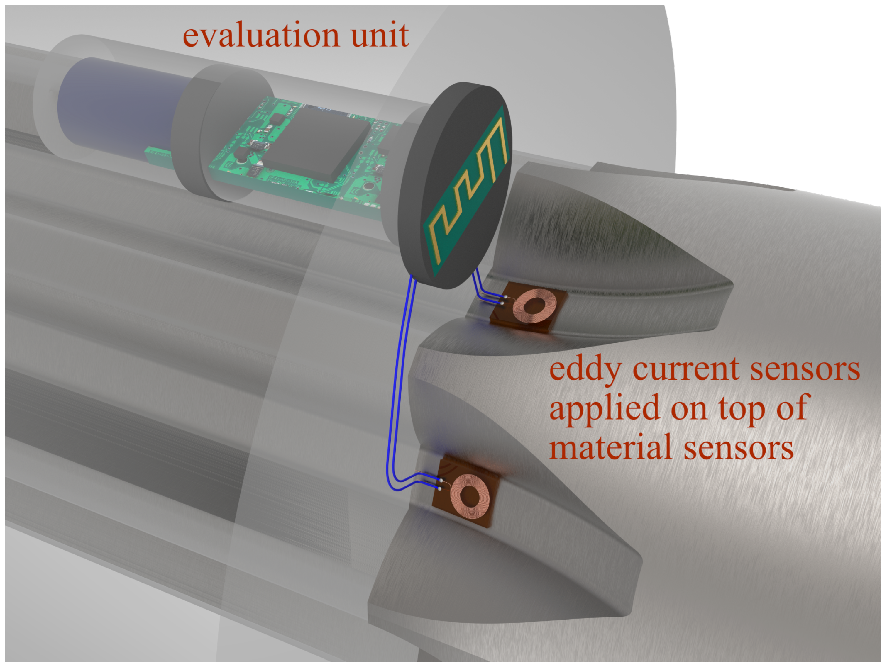
Figure 2.
Beraha II-etched microsection of a lasered lenticular sensor spot. Boundaries for computer modelling marked in red. Deformation structure, including martensite is black, austenite gold-colored. The mounting compound for metallography is dark greyish blue colored.
Figure 2.
Beraha II-etched microsection of a lasered lenticular sensor spot. Boundaries for computer modelling marked in red. Deformation structure, including martensite is black, austenite gold-colored. The mounting compound for metallography is dark greyish blue colored.
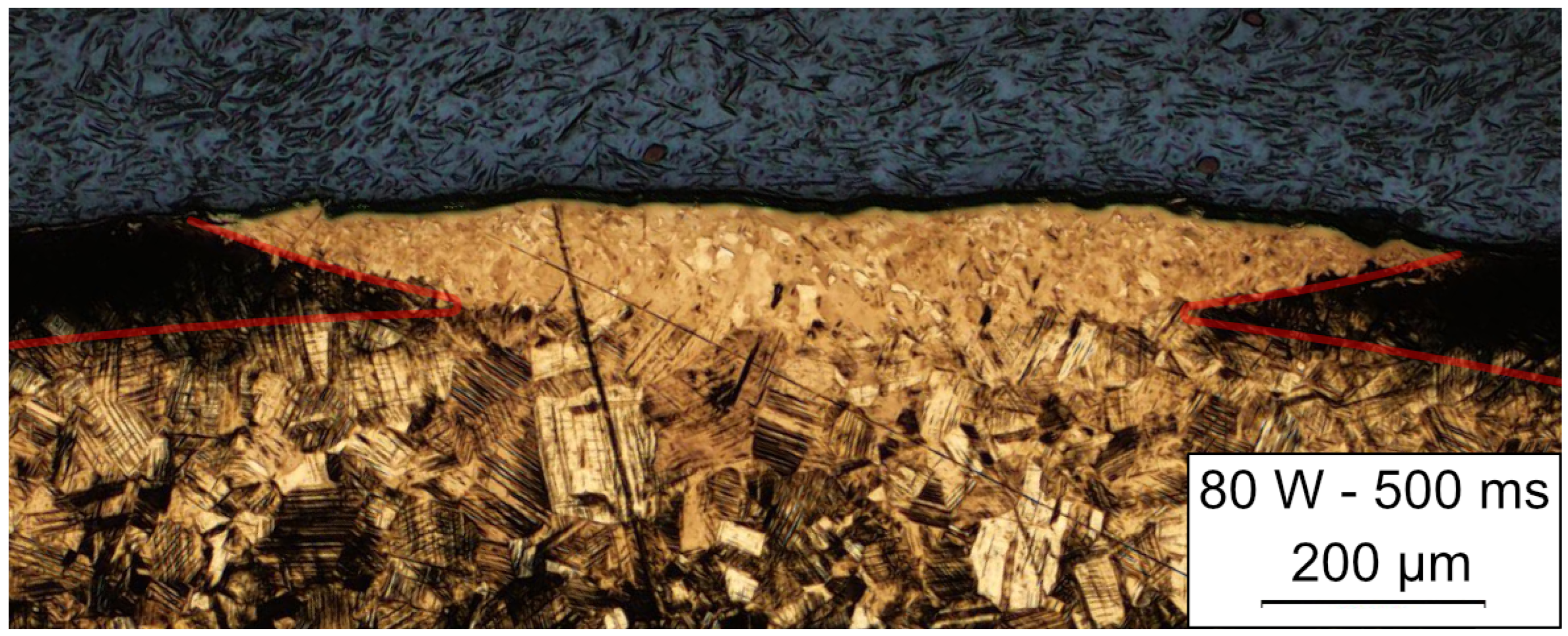
Figure 3.
simulated low-cycle fatigue test (8‰ strain amplitude) compared to experimental result. The experimental data are taken from Figure 96 of [12].
Figure 3.
simulated low-cycle fatigue test (8‰ strain amplitude) compared to experimental result. The experimental data are taken from Figure 96 of [12].
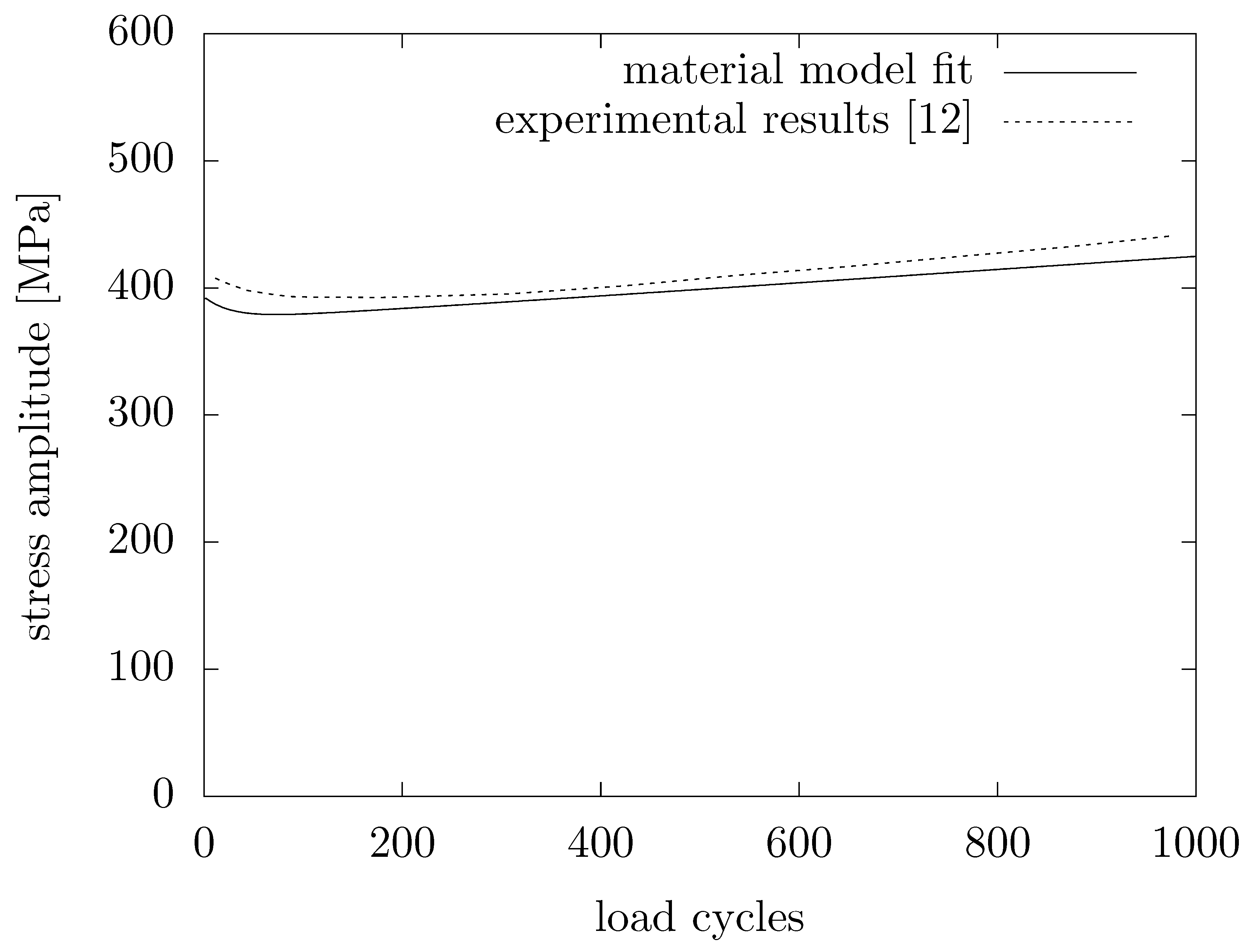
Figure 4.
geometrical model
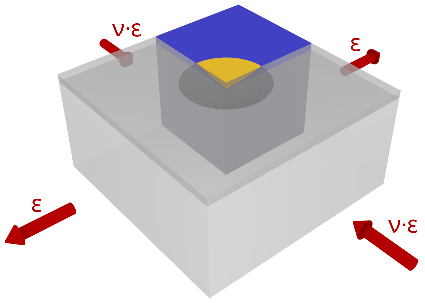
Figure 5.
Mesh with the XFEM boundary marked in red
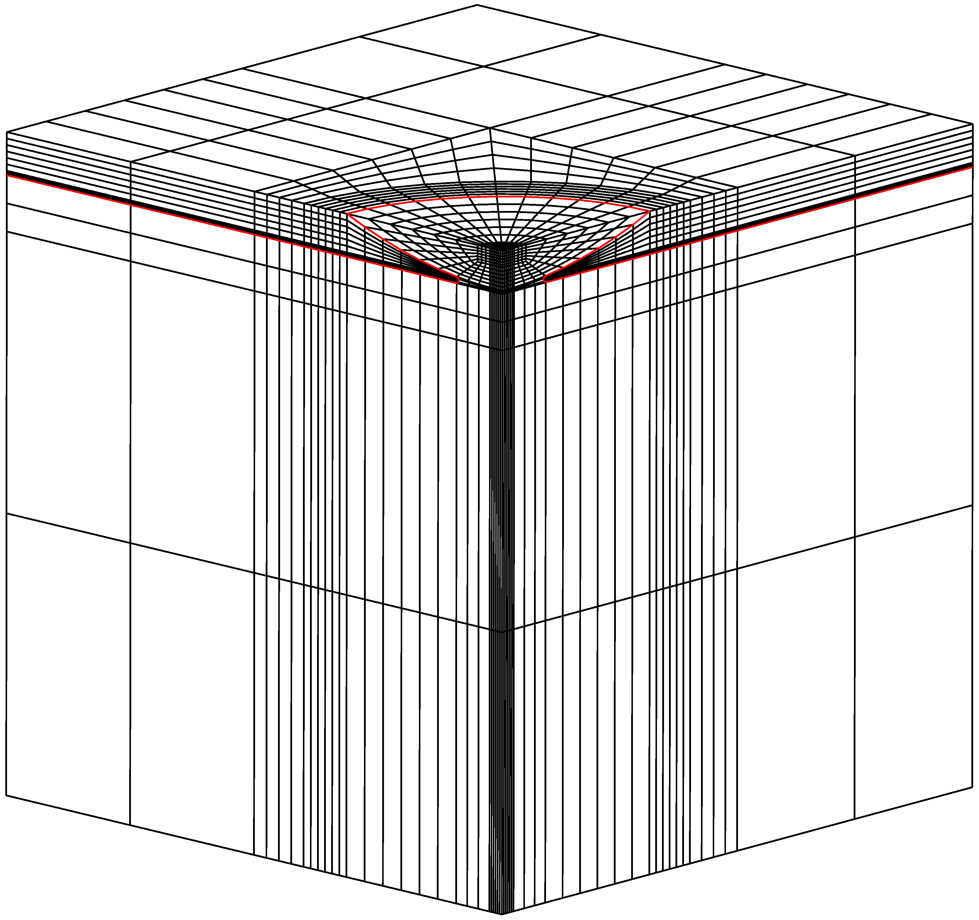
Figure 6.
initial state
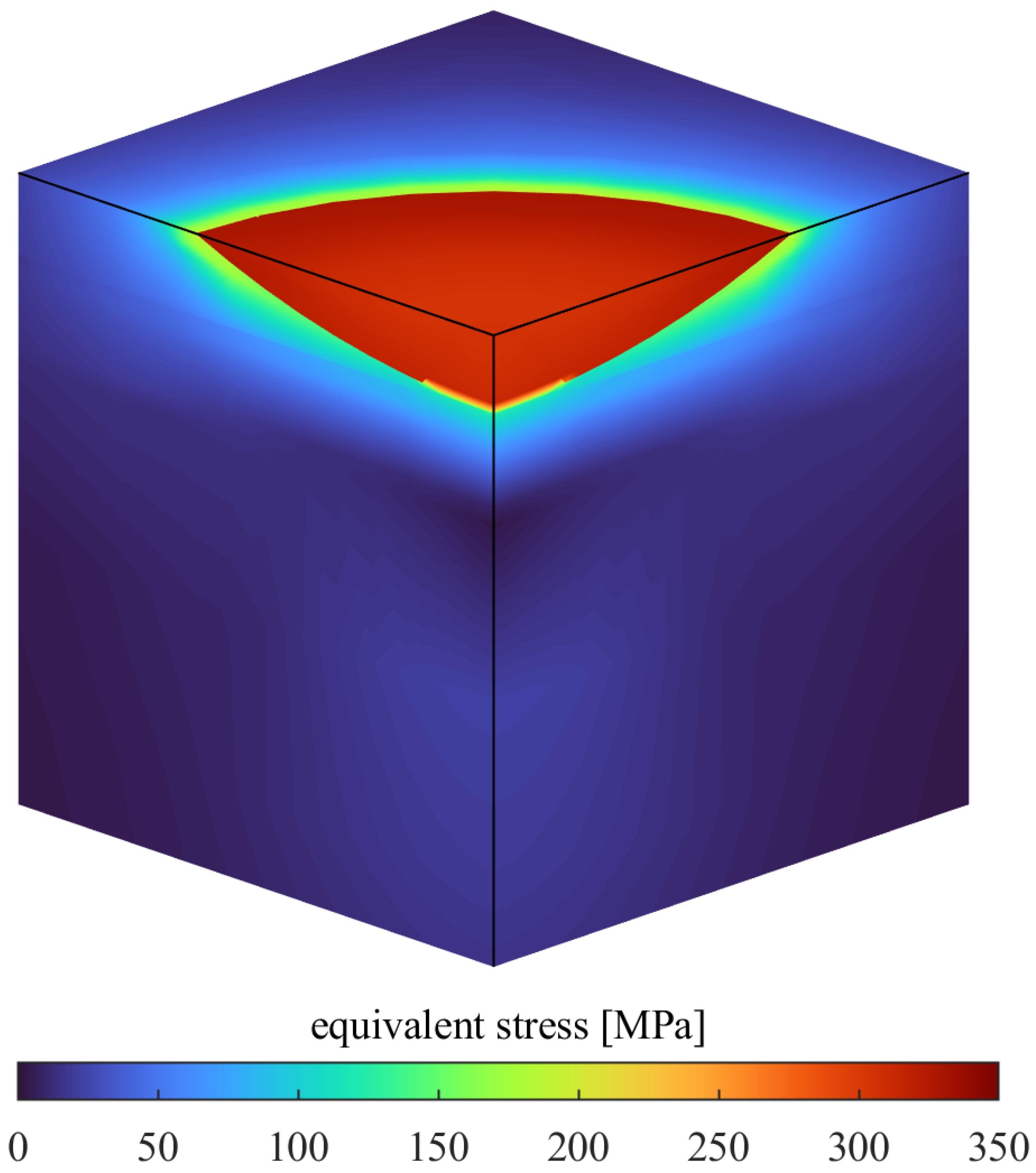
Figure 7.
single high and subsequent single low load amplitude
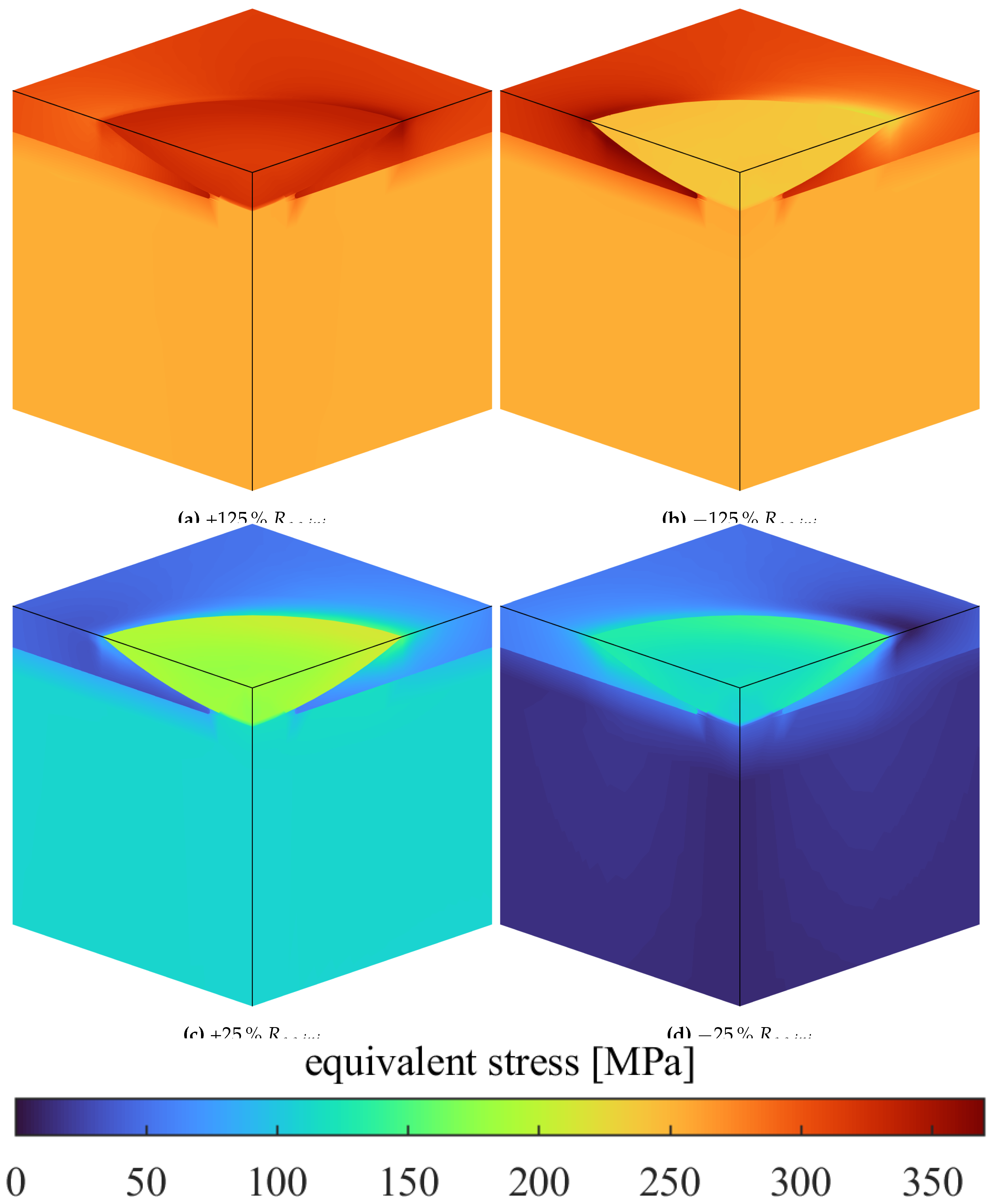
Figure 8.
stress factor at different overloads
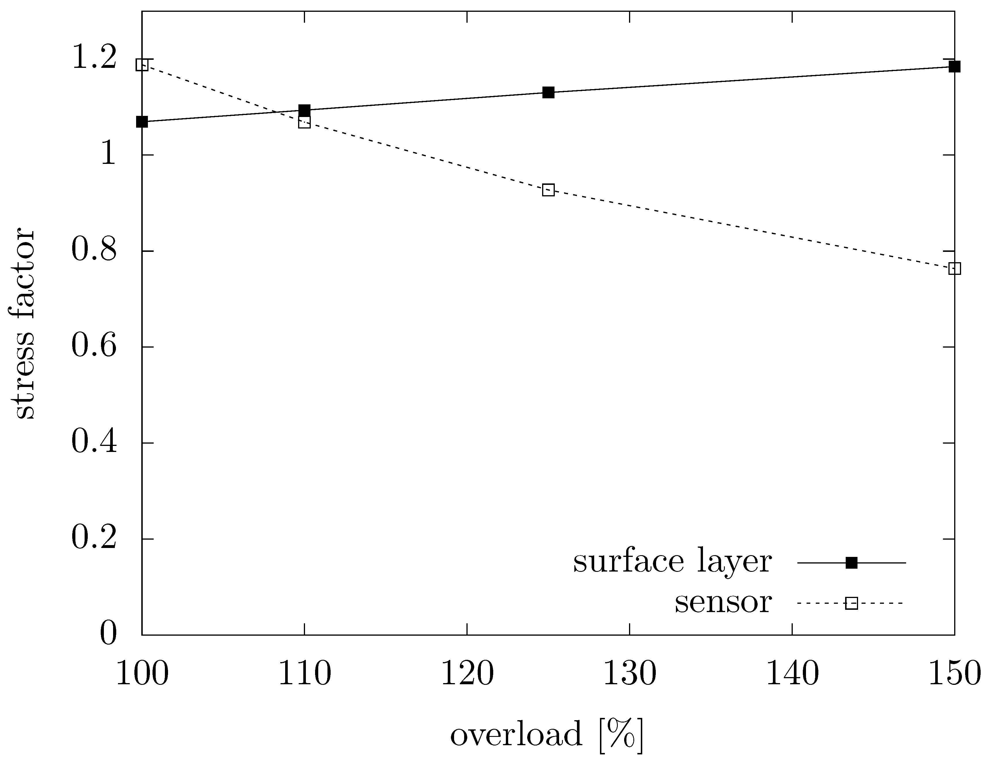
Figure 9.
martensite content at characteristic stages
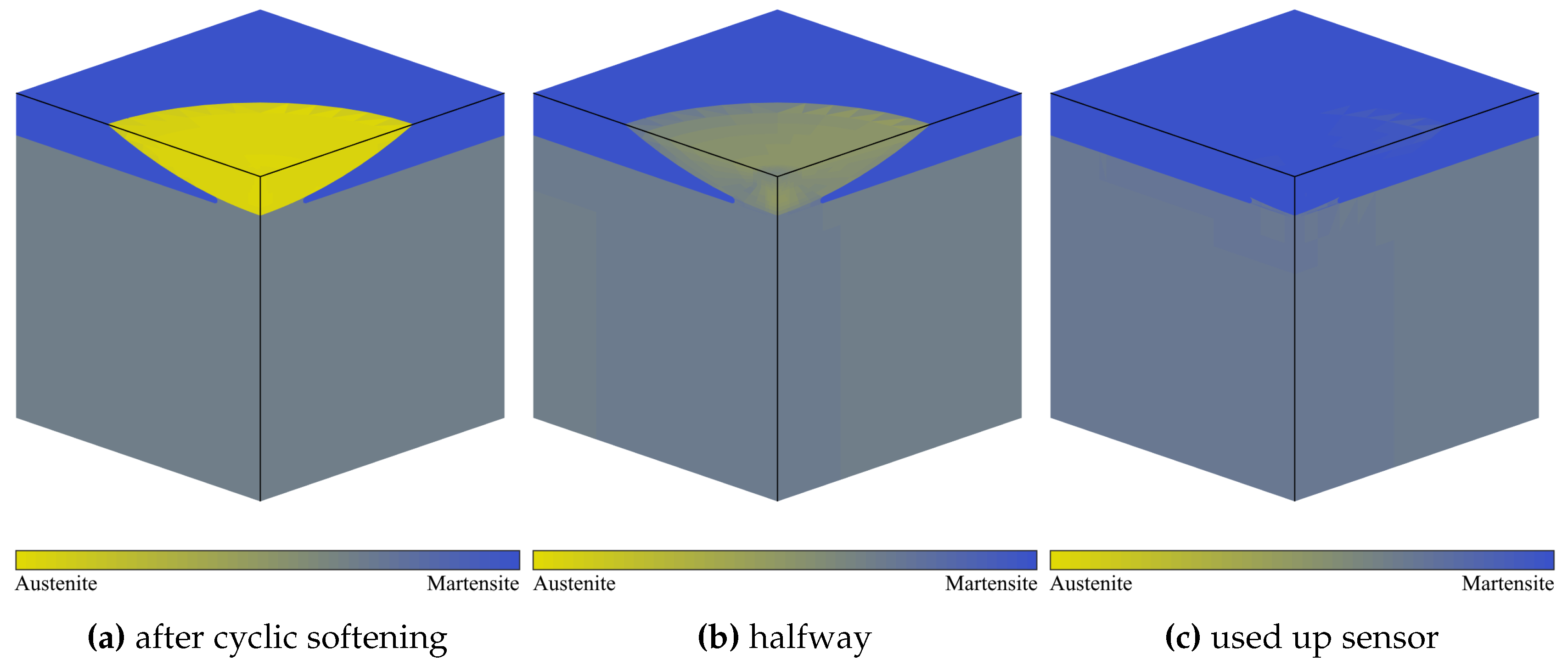
Figure 10.
residual stress at characteristic stages (without residual stress from shot peening)
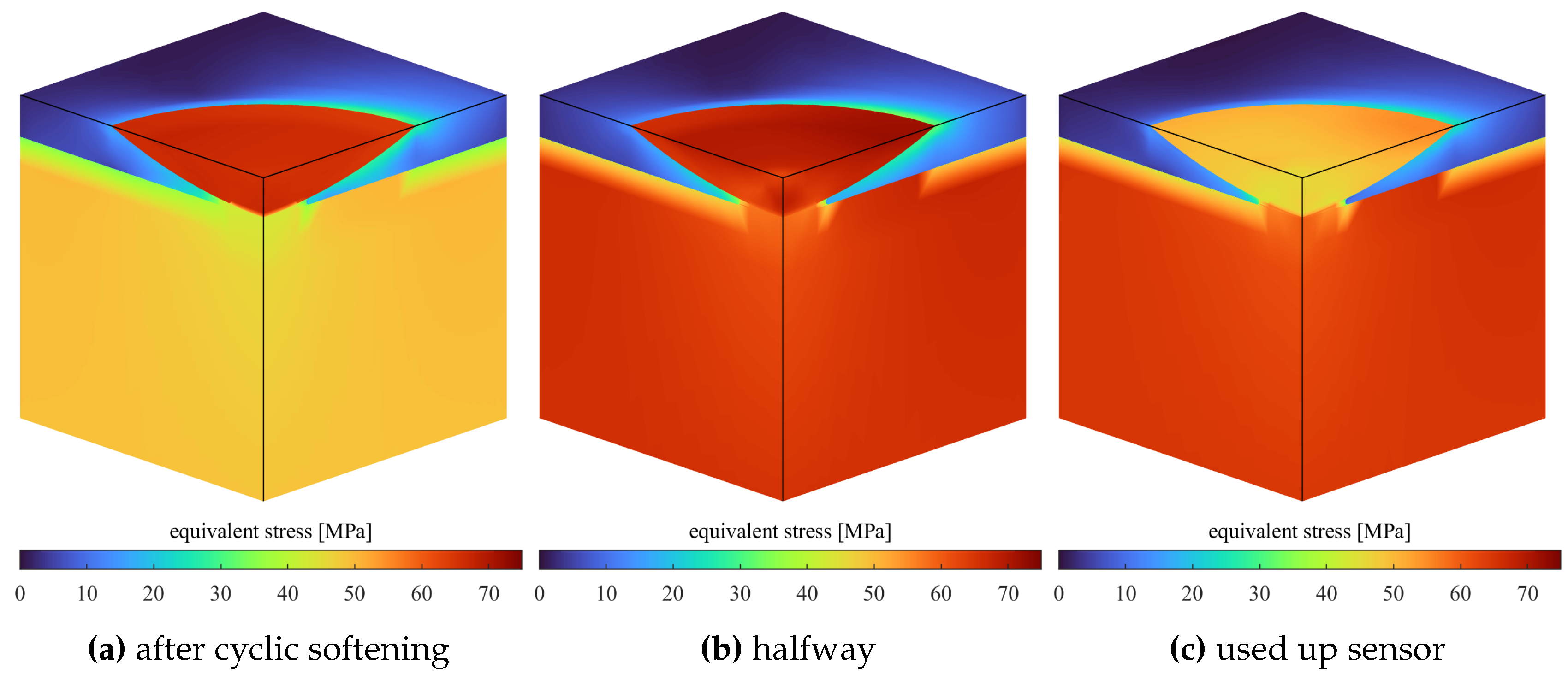
Figure 11.
stress under load at characteristic stages
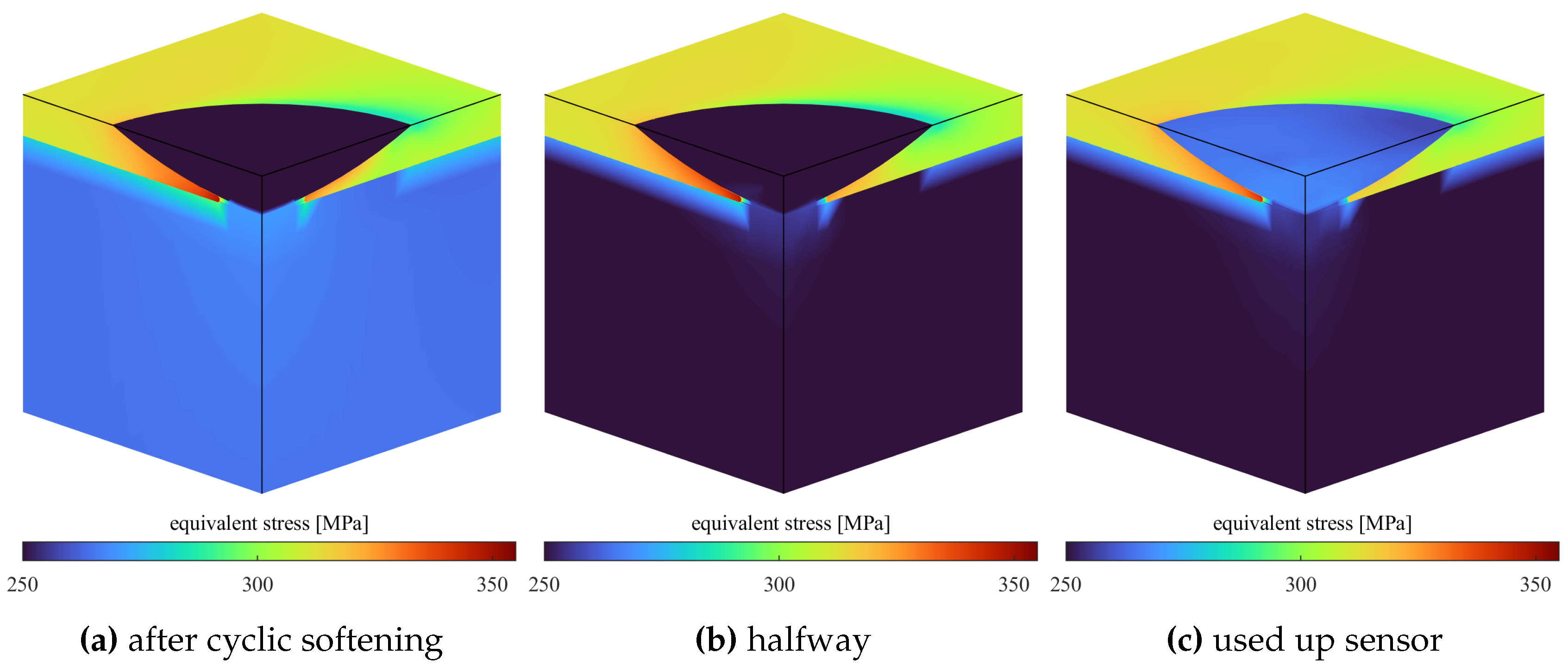
Figure 12.
stress and strain at the critical spot over load cycles (minimum values are negative before forming the absolute)
Figure 12.
stress and strain at the critical spot over load cycles (minimum values are negative before forming the absolute)
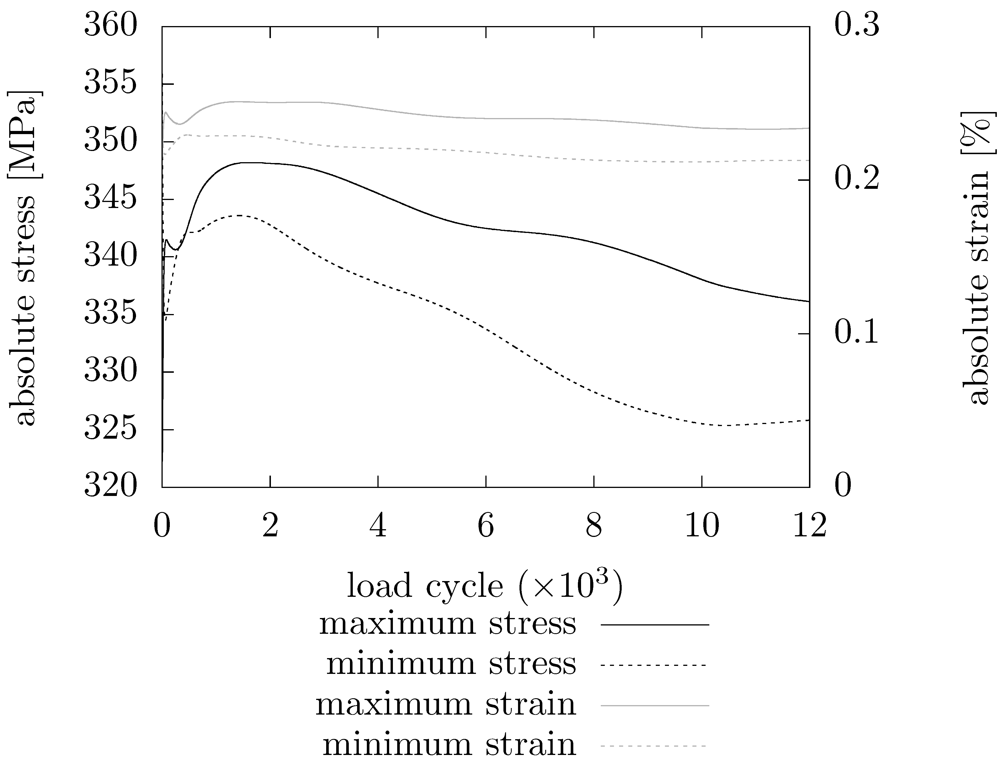
Figure 13.
cumulative damage at the critical spot over load cycles
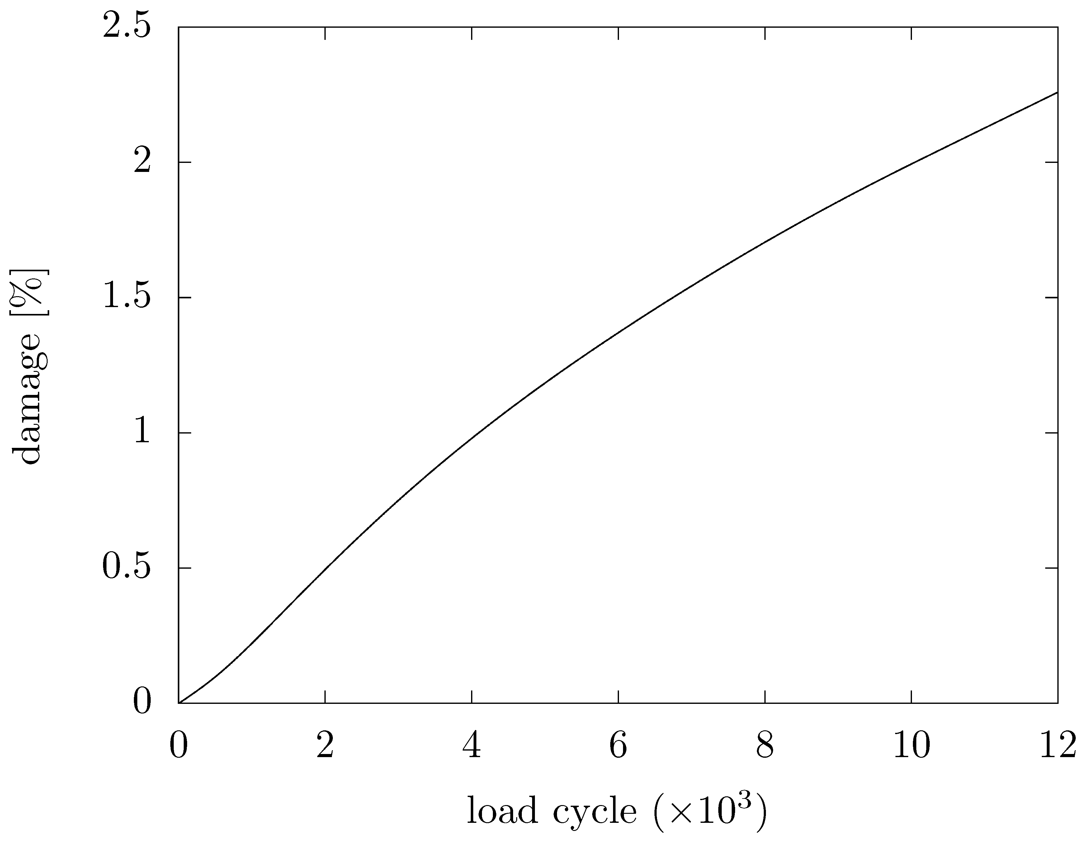
Figure 14.
martensite saturation level in the sensor over load cycles
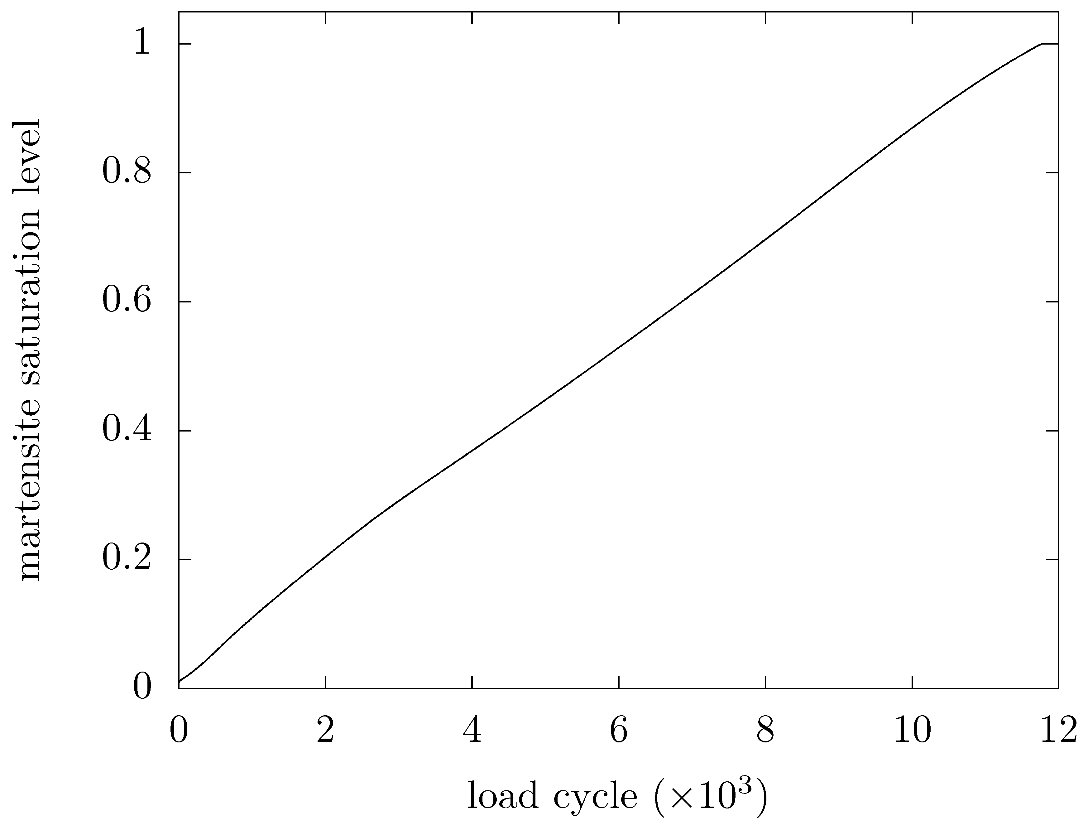
Figure 15.
no material in sensor volume (tensile load of 125% )
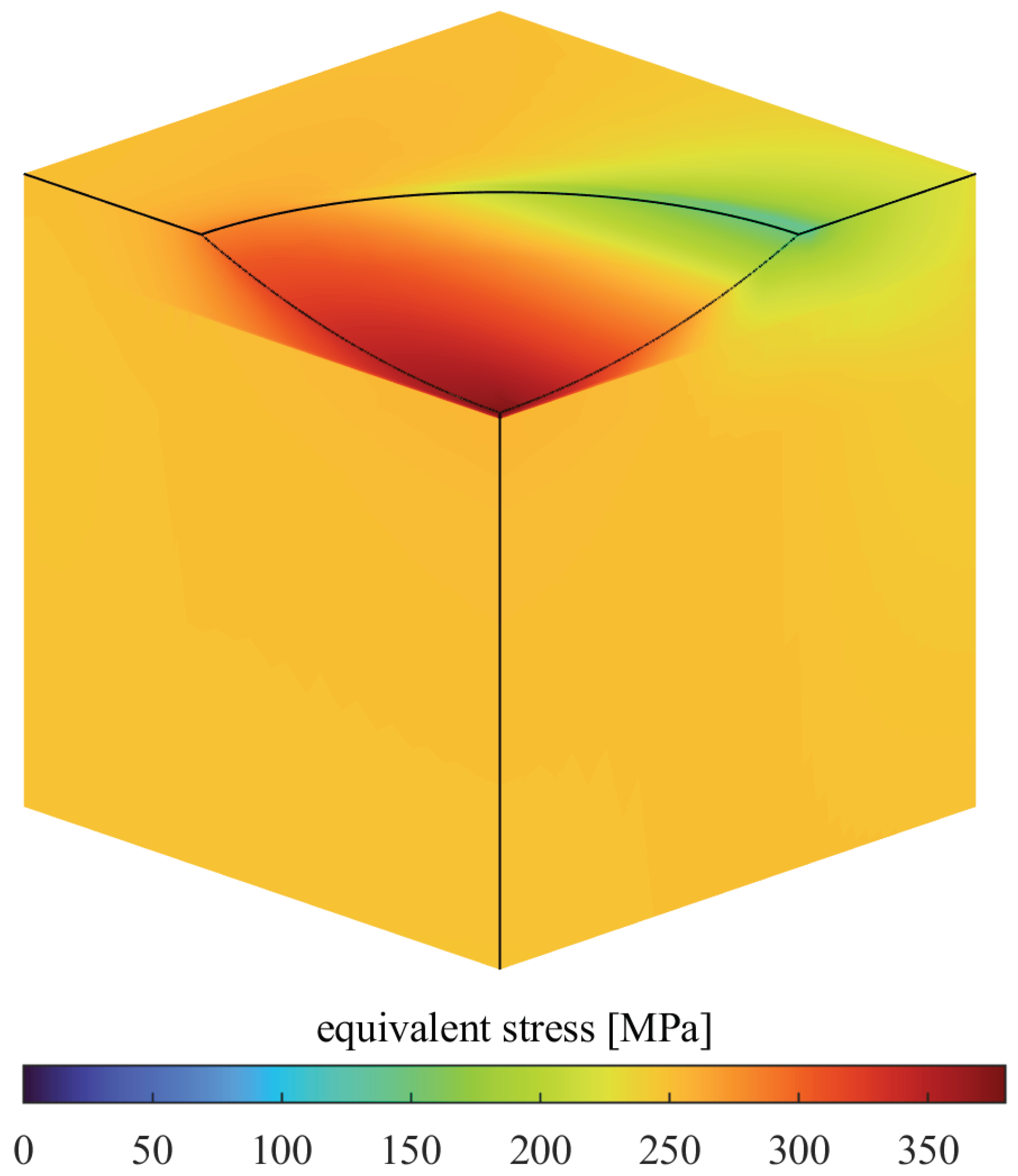

Table 1.
material constants (nomenclature acc. to [2])
Table 1.
material constants (nomenclature acc. to [2])
| coefficient | unit | Gallée [2] | this paper | ||
|---|---|---|---|---|---|
| austenite phase yield strength | 206 | 250 | ≈ | ||
| martensite transformation rate exponent | N | 2.2 | 2.4 | ≈ | |
| martensite transformation rate factor | 2.2 | 20 | ↑ | ||
| kinematic hardening factor | 11800 | 15000 | ≈ | ||
| kinematic hardening factor | 349 | 50 | ≈ | ||
| kinematic hardening factor | 136 | 50 | ≈ | ||
| isotropic hardening factor | Q | 1532 | −30 | ↓ | |
| isotropic hardening exponent | b | 1.12 | 0.4 | ↓ |
Table 2.
yield strength and martensite content after prestraining. Experimental martensite content from Table 7; experimental yield limits read off of Figs. 78, 81, 84 and 89 of [12]
Table 2.
yield strength and martensite content after prestraining. Experimental martensite content from Table 7; experimental yield limits read off of Figs. 78, 81, 84 and 89 of [12]
| prestrain | 0% | 5% | 10% | 15% | |
|---|---|---|---|---|---|
| unit | |||||
| yield strength experiment | 341 | 498 | 604 | 686 | |
| yield strength simulation | 308 | 516 | 619 | 729 | |
| yield strength | % | −9.7 | 3.6 | 2.5 | 6.3 |
| martensite content experiment | 25.6 | 31.9 | 36.6 | 47.1 | |
| martensite content simulation | 25.6 | 27.6 | 34.6 | 46.6 | |
| martensite content | % | 0.0 | −13.5 | −5.5 | 1.1 |
Disclaimer/Publisher’s Note: The statements, opinions and data contained in all publications are solely those of the individual author(s) and contributor(s) and not of MDPI and/or the editor(s). MDPI and/or the editor(s) disclaim responsibility for any injury to people or property resulting from any ideas, methods, instructions or products referred to in the content. |
© 2025 by the authors. Licensee MDPI, Basel, Switzerland. This article is an open access article distributed under the terms and conditions of the Creative Commons Attribution (CC BY) license (http://creativecommons.org/licenses/by/4.0/).
Copyright: This open access article is published under a Creative Commons CC BY 4.0 license, which permit the free download, distribution, and reuse, provided that the author and preprint are cited in any reuse.


