Submitted:
02 September 2025
Posted:
03 September 2025
You are already at the latest version
Abstract
Ohm's law has become ubiquitous in numerous scientific and technical disciplines. Generally, the subject is introduced to students in secondary school as fundamental technical knowledge. The present study proposes a visual model to facilitate the comprehension of Ohm's law in electron transport in solids to pre-university and university students. The objective is to facilitate students' comprehension of the correlation between electron movement in solids, as depicted by current, and the energy of the system, which is introduced by the electric field and the material's structure. The approach's originality lies in its novel strategy for describing electron trajectory randomization. This enables the establishment of a relationship between the material's structure and its resistivity. Moreover, the description of electron transport and scattering processes is presented in terms of different types of entropy. It is found that electrons follow maximum trajectory entropy and that thermal entropy presents a quadratic relationship with configurational entropy. The determinism of Ohm's law is inferred from statistical entropy.
Keywords:
Ohm’s law
; entropy
; randomization
; determinism
; Joule effect
; dissipation
; relaxation time
1. Introduction
Georg Simon Ohm published the homonymous physical law that relates electrical current, voltage and resistance in 1827. To commemorate the close bicentenary Connelly has recently published a thesis that provides a contemporary explanation of the original research [1]. In the 1891 translated edition [2], three interesting ideas can be identified. Firstly, Ohm attempted to derive the law in parallel with Fourier’s conduction law. Secondly, a note from J.C. Maxwell indicated that this was a mistaken approach; and thirdly, a comment in the preface from T.D. Lockwood stating that “many quote Ohm’s law and talk about Ohm’s law, who know little or nothing of Ohm himself, or of his book”. The first idea can be interpreted within the framework of irreversible thermodynamics, wherein Ohm’s law, in conjunction with Joule effect, elucidates entropy generation in dissipative processes[3]. Conversely, the pervasive use of Ohm’s law in engineering confirms that it has been completely decoupled from the original thermodynamic approach, as Maxwell observed.
The most widely accepted interpretation of Ohm’s law is that the material opposes the flow of an electrical current when subjected to a voltage. However, the manner in which the material exhibits this resistance is unclear from the general expression (1). Various approaches have been suggested to explain this relationship (see Table 1). The original approach describes Ohm’s law as a proportionality through a resistor, which must be determined experimentally. When the geometry of the material is introduced, the resistor can be split into resistance, section and length. Resistance is an intrinsic parameter of the material (illustrated in equation 2). Drude proposed a model based on electron collisions which evolve from a constant R to a constant τ, related to the relaxation time of the electrons in the solid (see equation 3). At present, electron transport in solid-state physics books [4,5] is described in terms of band theory and of Boltzmann equation. This equation is based on the conservation of momentum of a free electron gas scattering in the solid. It is difficult to solve unless simplifications are assumed. A common simplification consists of considering the linearization of relaxation time. Also, local thermal equilibrium and the fact that collisions are completely effective in obliterating any information about the nonequilibrium configuration that the electrons may be carrying [4,5] help to find an analytical solution of (4).
As mentioned above, there is a relationship between entropy generation and Ohm’s law. Entropy measures the uncertainty of a system. Entropy was historically introduced by Clausius to study the performance of thermal machines, which led to the formulation of the second law of thermodynamics. More recently, Boltzmann related entropy to the available states of a system within the framework of statistical physics. It has been proven that these two approaches are equivalent [6]. This is reasonable, as both expressions define the probability of the thermal system from different points of view: macroscopic in thermodynamics and microscopic in statistical physics. Planck studied the entropy related to the probability of energy availability in oscillators [7], which led to the birth of quantum physics. Shannon generalised Planck’s entropy by averaging probabilities and applied it to information transmission [8]. It is important to understand here that all entropies measure the same thing: the probability of a system’s property. However, it is also worth pointing out that, whereas the entropy of a thermal system measures energy probability, Shannon entropy measures the probability of information transmission quality. More refined general mathematical expressions were later derived, such as Tsallis [9] or Rényi [10], of which Boltzmann, Planck and Shannon are limit cases.
Ohm’s law is introduced to students’ curriculum in secondary school. As found in the literature, the physical comprehension of Ohm’s law, as derived from a solid-state approach, is rather complex. The available model conceptualises electron collisions as random processes, in such a way that after each collision, previous information is obliterated. Furthermore, the utilisation of differential equations, founded upon time evolution, is employed for the analysis and prediction of outcomes. While differential equations are a convenient tool for the description of deterministic systems, their application to random processes is typically intractable, as evidenced by the attempts to solve (4). Finally, the reason behind introducing entropy in this context stems from Feynman’s suggestion that Ohm’s law should adhere to a minimum entropy trajectory. However, this approach remained unexplored [11].
Thus, the aim of this study is to propose a straightforward model for the visualisation of electron transport in conductors, with the intention of facilitating comprehension among pre-university and university students. The model introduces a novel randomisation strategy for the analysis of electron trajectories, with the constraints of momentum and energy conservation. For convenience, entropy is utilised to evaluate the randomness associated with collisions. This approach recovers Ohm’s original approach to a dissipative system, and it further incorporates entropy concepts that emerged subsequent to Ohm’s contributions. Obviously, given the well-established nature of Ohm’s law within the domain of physics, characterised by its deterministic and causal nature, it is essential that the model incorporates these features.
The objectives of this manuscript are:
- -
- To develop a simplified model that explains electron conduction in solids through Ohm’s law, the Joule effect, and the associated entropy changes.
- -
- To establish a multiphysics framework aimed at helping both pre-university and university students gain a deeper understanding of the role of random process in physics laws, in particular, in Ohm’s law.
The scope is to facilitate a visual comprehension of electron transport for students at the pre-university and university levels. In Spain, the physics curriculum for students around 13 years of age encompasses an introduction to the structure of matter (protons, electrons, and neutrons), energy (mechanical and electrical), and forces (mechanical and electrical). Within the discipline of mathematics, students receive a brief introduction to fundamental probability concepts, encompassing combinatorics and the Gaussian distribution. Following the introduction of mechanical energy, the concept of Ohm’s law is introduced through simple electric circuits. With respect to university undergraduate students, they are familiar with probability theory, with a particular emphasis on the Gaussian distribution. Their studies have encompassed atomic models and the associated concepts of energy and entropy. Furthermore, they possess a comprehensive understanding of fundamental principles, including the conservation of momentum and energy, as well as the familiarity with elastic and inelastic collisions.
2. Materials and Methods
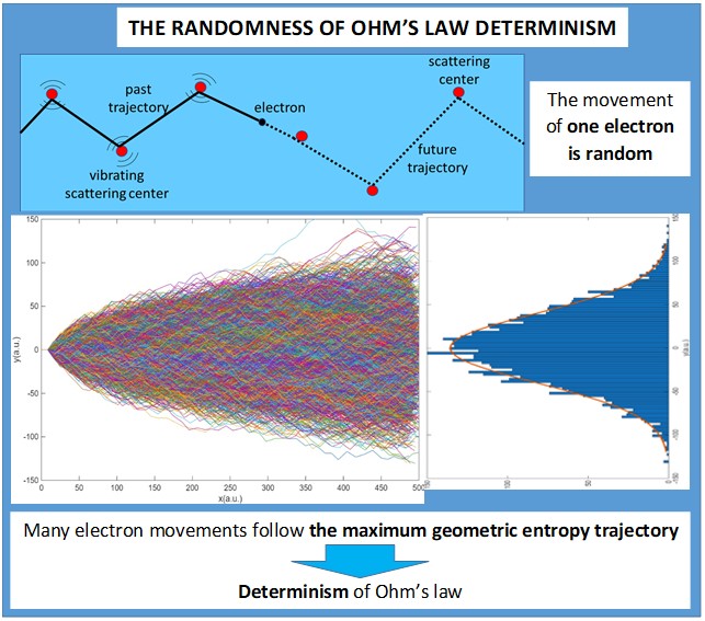
The model’s methodology is inspired by the Galton board [12] (see Figure 1a for an illustration). It is assumed that the electrons follow a specific trajectory from the starting point (the negative electrode) to the end (the positive electrode). This trajectory depends on collisions within the material, which are randomly distributed along the path. Rather than taking the classical differential approach to study how electrons move from one point to the next in a given time, we adopt an integral approach, considering the final two-dimensional trajectory of each electron (see Figure 1b). The critical difference between the two approaches lies in how randomisation is performed in the transition from the mechanical to the statistical approach. In statistical models, such as those explained in Table 1, randomisation is carried out for every collision at each instant in time. In this approach, we retain prior information relating to the previous collision for each electron and project it into the future. As in the theory of probability, time is less relevant than in classical physics. This means that we do not observe what the electron does at each moment, but rather we take a broader view of what it is expected to do overall. This gives us a general picture of an electron’s behaviour, enabling us to obtain the current from the sum of all the electrons’ trajectories. Finally, it is worth explaining how the trajectories are set. Electrons are known to move from one electrode to another due to the electric field. The electric field introduces a privileged direction, favouring collisions in this direction. Unlike pure random collisions (4), collisions are random, but those aligned in the direction of the field are more probable. Figure 1c illustrates how an electron absorbs energy from the field in the privileged direction and transfer it to the lattice in a random direction.
The following assumptions are considered:
- -
- Each electron and each trajectory are independent of the others (free electron gas approximation).
- -
- Collisions occur against collision centres, of which only the impact point, radii and its mass are considered.
- -
- The velocity along the X-axis (i.e., in the direction of the electric field) remains constant prior to the next collision; otherwise the current would not be constant. This simplification implies that no back collisions are considered in this approach, but no loss of generality occurs.
- -
- The velocity in the Y-axis depends on the energy dissipated in each collision, and then reabsorbed from the field between collisions.
- -
- The density of scattering centres is a material-specific characteristic.
- -
- Collision centres are located at a distance R ± X·d where -1 < X < 1 is a random number and d is chosen to be 20 % of R. Thus, the collision centres are randomly distributed at a constant average distance R ± 20 % in order to consider that scattering centres can move due to thermal vibrations, diffusions or any other dynamic process.
- -
- Two dimensions for collisions are assumed. One dimension would imply either a superconductor or a blocked trajectory by the scattering centre. The extension to three dimensions of these model is straightforward.
- -
- Electrons have memory, introduced by the privileged direction of the electric field. They do not obliterate past information related to previous collisions.
Once the assumptions are fixed, we propose the following steps to evaluate Ohm’s law, as graphically schematized in Figure 2. The numerical simulations are carried out with Matlab©.
Step 1 – Location of random centres:
Random centres are located at an increasing X, and random Y using the expression:
α, γ are indexes randomly changing between 0 or 1, to have positive or negative variation with respect to the average distance change d. β and δ are random decimal numbers between 0 and 1. c is a constant limiting the variation range around d. In our simulations, we choose 0.2, so that the points are located at an average distance d±c d in the X-axis. With respect to the Y-axis, the following collision can only take place within the range ±c·d from the previous collision. Thus, starting from point (x,y)=(0,0), we create an array of numbers with an average distance (+d ±c d,. ±c d).
Step 2 – Simulate the movement of electrons, one by one, by imposing:
- -
- A definite number of collisions.
- -
- A definite number of electrons.
Step 3 – Analyse the momentum that is transferred to the atoms of the network (collision centres)
And the energy that is transferred to the atoms of the network (collision centres)
m* is the effective mass of the electron, mc the mass of the collision center, vei the input velocity of the electron prior to the collision and veo and vco the velocities of the electron and the collision centre after the collision.
Step 4 – Impose Ohm’s law and Joule effect to each one of the paths that different electrons follow, in terms of position, momentum and energy, to find the voltage field profile.
Step 5 – Evaluate the entropies of the trajectory and of the energy (details provided in next section).
Current is defined as where n is the electron density, e- the charge of the electron, v the velocity moving between electrodes and A the area of the electrodes. It is worth recalling the parallelism between moment (6) and energy (7) equations and Ohm’s law and Joules’s law
Knowing that the I is proportional to v. Current and momentum are linear with velocity whereas energy is quadratic in both cases. For their part, the electrons lose energy in each collision. But after colliding, they take some energy back from the electric field to continue moving at the same speed in the X direction, so they always impact the next atom with the same vx (see Figure 1c). Using Joule effect where t is the time that takes the electron to complete its trajectory and Ediss the dissipated energy during the trajectory, which is the original energy that the electron had at the negative electrode. Substituting
We obtain the resistance of the material of length L.
2.1. Determination of Entropies
The entropy expressions used in the results analysis are briefly introduced here: Shannon entropy, thermal entropy and statistical entropy.
2.1.1. Shannon Entropy
Shannon entropy is given by
where S is the entropy and P is the probability of an event. In the original work [8], the probability was referred to information. In our work, however, we simply consider a general probability. In the case of an electron’s trajectory, P represents the probability of it taking one path or another at each collision, as in a Galton machine. Different types of probability can be defined. Following the histograms in Figure 4, the probability of deviating from the X-axis PY can be written as:
where DY is the collision distance from the x-axis and D is the distance between particles as illustrated in Figure 3. Also, the geometrical probability Pc of the subtended angle αc (between to consecutive collision points with respect to the x-axis) can be considered:
π is taken as the total angle because no backward collisions are considered in the model. In the geometry, it is assumed that the distances between collision points are much larger that their size.
Figure 3.
Geometry of the collision between the electron (circle in red) and the scattering centres (circles in blue). The green line represents the trajectory of the electron that collides with particle 1, and α1 is the angle with respect to the x-axis. The black solid lines show the distance between the collision centre and the electron. The black dashed lines, with angle αmax corresponds to the maximum angle subtended by the scattering centre.
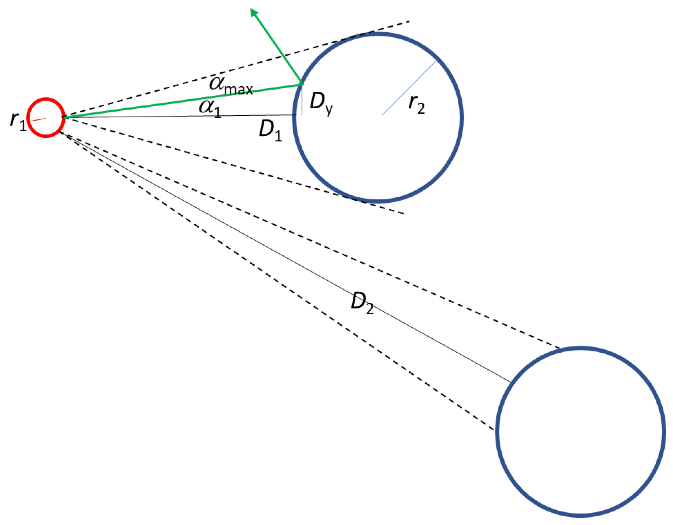
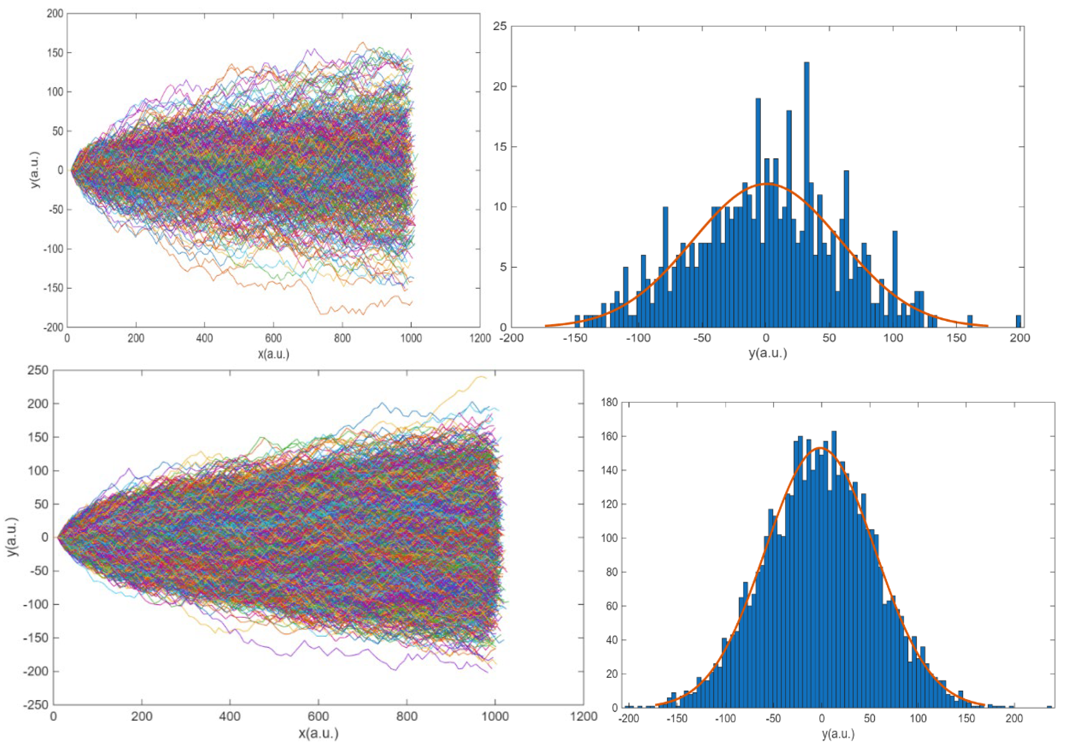
Figure 4.
a) Pre-defined trajectory of one electron with random scattering centres from left to right. The red and yellow straight lines are the limit the maximum Y in each position. b) trajectories of 500 electrons colliding 100 times. c) histogram of the final positions in the y axis in (b) with m=-1.57 and σ = 57.06. d) trajectories of 5000 electrons colliding 100 times e) histogram of the final position in the y axis in (d) with m=-1.57 and σ = 57.06.
2.1.2. Thermal Entropy
The thermal entropy generation at a resistor due to the energy conversion from electrical to thermal is given by [3]
where V is the voltage drop at the resistor, I the current and T the temperature of the resistor and t the integration time.
2.1.3. Statistical Entropy
When large amount of data is described by gaussian distribution, the entropy of the distribution represents the degree of dispersion of the samples. Its entropy is given by [13]
where σ2 is the variance of the gaussian.
3. Results
Following the strategy pointed out in the methodology, the results for the electron transport between electrodes are illustrated in Figure 4. In a) the trajectory of a single electron is plotted once the scattering centres have been generated. The electron follows a random trajectory travelling from the negative electrode towards the positive electrode attracted by the voltage drop. Obviously, one electron does not define Ohm’s law. Simulations with 500 and 5000 are illustrated in Figure 4b and d. Each electron follows a random trajectory between electrodes as the one described in a). This trajectory is independent of the other electrons. Their distributions with respect to the origin are illustrated in the histograms (Figure 4 c and e). It is evident that as the number of electrons increases, the trajectories are distributed in a Gaussian with respect to the Y direction. The mean of this distribution is equal to zero, and the variance is dependent on the geometry.
Once the trajectory of every electron is established, the power transferred to the lattice can be estimated from the energy losses at each collision with the scattering centres, as described in equations (6) and (7),
Where t is the time between collisions and τ the relaxation time. This is an interesting result because it allows to infer the relaxation time. Relaxation time is the time that takes the electron to absorb energy from the field and recover the v of the steady state. Simplifying for one electron:
In order to keep a constant resistivity ρ, this equation must be time-independent, otherwise, a change in the current (proportional to v) would lead to a change in the resistance, which is not possible to solve Ohm’s equation. Thus, it is necessary that:
where k is a constant. This means that the relaxation time is linear with the collision time. This result may seem arbitrary at first glance, but we can consider the following interpretation. As both times are proportional, it means that
Where l is the distance between scattering centres and lmean is the distance required to reabsorb energy from the field. It is reasonable to think that, as the electron is moving at a certain velocity to reach the next collision, it also relaxes at the same velocity in a shorter range. This is helpful to understand the different definitions of τ found in literature, such as the time between collisions [4], the sums up of all scattering events [14] or relaxation time, i.e., the time to reach thermal equilibrium (or constant vx in this case). In these conditions, dissipated energy is proportional to k, and thus, it is related to the geometry defined by the trajectory.
Determining k for each case, we can recalculate R using (10) and then, find V=R·I.
where α is the angle between the trajectory and the X-axis. This expression relates the voltage with the geometry of the scatter centres. Thus, we found the connection between the geometry of the material and the electron transport which match with the electrical observations: Ohm’s law and Joule effect.
4. Discussion
The implications on entropy in Figure 4 are of considerable significance and deserve detailed discussion. We consider implications on: characterizing the deterministic behaviour of Ohm’s law, the preferred trajectories of the electrons, the energy transfer to the lattice, and the relationship between the geometry of the material and the opposition to current flow.
First, we consider the profile of the distribution on the histograms. The distribution is found to be gaussian, due to the randomness of the collision. According to Jaynes [15], the gaussian probability distribution is the one with larger entropy for a given mean and variance, for which it is useful to describe random processes. The scattering centres were simulated by means of the Matlab functions rand and randn, whose function is to generate random numbers that are uniformly and normally distributed respectively. No discernible difference between both types of geometries is observed. Furthermore, the gaussian distribution is also achieved if the scattering centres follow a regular pattern, as in the Galton board shown in the methodology, where the separation between the centres is constant. Thus, the randomness of the collisions is independent of the configuration of the scattering centres. With respect to the properties of the distributions, the mean and variance of the probability distribution are independent of the number of points. It can thus be concluded that the entropy of the probability distribution, as defined for Ss (13), depends on the distance between scattering centres, but not on the number of electrons. This is illustrated in Figure 5, which shows the relationship between the distance between collision centres and the entropy of the probability distribution, Ss.
It is also interesting to note that, in the context of Gaussian distributions, the relationship between the mean, the variance, and the number of particles is expressed as [15]:
and describe the fluctuations δX with respect to the average <X> of a magnitude X. Hence, the behaviour of one electron is purely indeterministic whereas for a system of a large number of electrons, fluctuations decrease, and the system becomes deterministic, an expected behaviour of Ohm’s law.
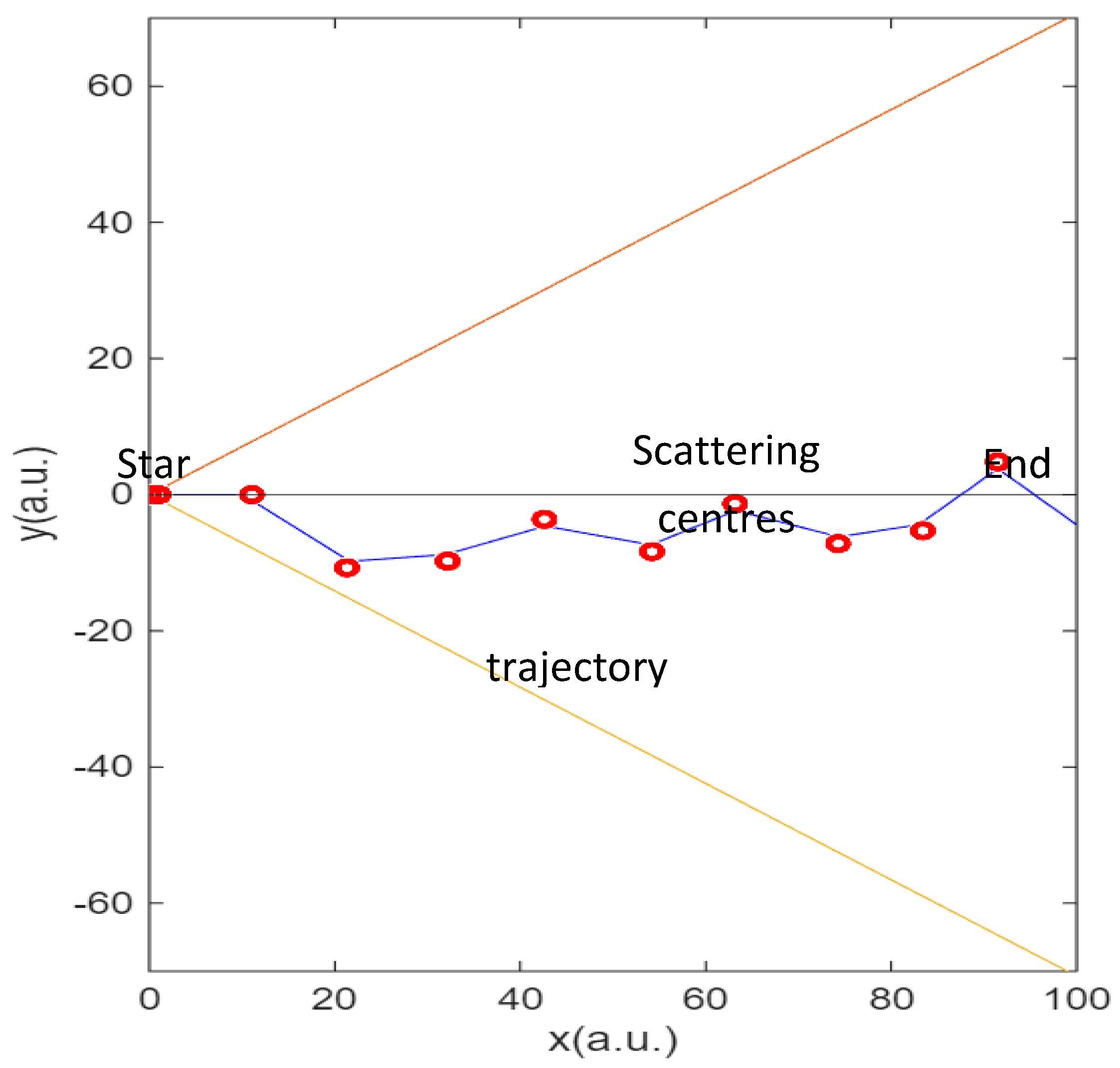
Second, as stated in the methodology, the description was inspired in the Galton board. Each trajectory can be described by the angles of collisions. Thus, we can digitalize the trajectory by assigning 1 if the collision deviates the electron up and assign 0 if the collision deviates the electron down. Each trajectory will have the same total collisions as imposed in the model. The extreme ones (orange and yellow lines in Figure 6) will be a digital word with all numbers equal (00..00 for the yellow one and 11..11 for the orange one). Those trajectories reaching the mean have the same number of collisions up and down and are the most common, as seen in the histograms. We calculate the entropy of the digitalized series as the ratio of times it goes up (Y>0) or down (Y<0) using expression (11) to obtain the trajectory entropy ST. If all the collisions are in the same direction, the ST = 0. If there are as many in one direction or the other, ST is maximum. This is graphically illustrated in Figure 6.
Thus, in the case of a very large number of electrons, the fluctuations decrease, favouring the most probable trajectories, which are those with maximum ST, i.e., the most probable trajectories are those with the greatest entropy trajectory entropy ST. These two facts allow for the visualisation of the movement of electrons: they are constantly colliding to go up and down and move through a kind of channel close to the mean, the one that offers the maximum entropy of the trajectory. The distance traversed by the maximum ST path is equivalent to the minimum distance from the origin (See Figure 6) whereas the longest distance corresponds to the minimum ST.
Third, we discuss the thermal entropy in the problem, that is, how the energy of the electrons is transferred to the lattice. The electrons flowing in the electric field collide with the scattering centres, whom they transfer energy. This energy increases the thermal entropy of lattice. After the collision and before the next collision, the electron reabsorb energy from the field, to keep the constant velocity and start the same process in the next collision. Thus, we can recover the classical expression of entropy generation in electric circuits [3]:
This expression shows the link that Ohm’s law is close related to Joule effect during current flow through a solid conductor.
Finally, following the philosophy of the manuscript of calculating probabilities and entropies, the last analysis relates the configurational entropy of the material with thermal entropy, i.e., we aim to understand how electron’s energy is dissipated as a function of material structure. To obtain thermal entropy Si, we integrate (11) over time. The configurational entropy is obtained using (13) from the probability of collision as a function of the angle (calculated using (11)). A quadratic relationship between thermal entropy and configurational entropy is found, illustrated in Figure 7, and thus proving the causality between them. This quadratic relationship is also dependent on the distance between scattering centres through the geometric probability Sc. This final figure illustrates how electrons moving over a geometrical structure, the conductor, in the presence of an electric field obeys momentum conservation and energy conservation. This relationship clarifies the usual concept “opposition” that that current undergoes when flowing through a resistor. Summarizing, as there is a correlation between entropies, as between thermodynamics and statistitical physics, entropies are causally related [16].
We had carried out experimental measurements on resistors to study their degration mechanisms [17]. Ohm law and Joule effect were satisified and evolved with degradation, which was explained in terms of thermal entropy. However, the best model at the moment was based on unified mechanics theory [18] but it failed to relate the internal structure evolution with the thermal performance. Our present model has solved this issue by relating configurational entropy to thermal entropy.
With respect to the utility of the model for pre-university and university students, it can be useful for:
- -
- Introducing entropy linked to probability intuitions to understand real world, beyond the limited use to thermal machines. Also, in contrast to the usual understanding of Physics in terms of forces it would be possible to describe it in terms of energy and entropy, facilitating the Multiphysics comprehension.
- -
- Introducing collisions (moment and energy conservation in mechanics). Though the model considers collisions, their analysis can be introduced qualitatively in pre-university courses and quantitatively in university courses.
- -
- Introducing transport properties in solid state courses.
Last, but not least, this probabilistic approach could serve for a better understanding of quantum mechanics courses and artificial intelligence courses. For our research, it must be helpful to develop battery degradation models.
5. Conclusions
The proposed model to describe Ohm’s law has provided a simple understanding of nonequilibrium electron transport in a resistor based on the relationship between the entropies present in the problem: the configurational entropy, the statistical entropy and the thermal entropy. It was concluded that:
- -
- Electric current in Ohm’s law follows the maximum configurational entropy trajectory, thus becoming a deterministic problem.
- -
- The large number of electrons favour a gaussian distribution with smaller fluctuations (electrical noise).
- -
- The model satisfies the goal of the manuscript of achieving a simple visualization description of Ohm’s law that can be useful to pre-university students. The introduction of probability concepts in elementary physics provides a deeper understanding of the physical laws.
Author Contributions
“Conceptualization, A.C., M.C.A., G.C.A; methodology, A.C.; software, A.C.; validation, A.C., M.C.A., G.C.A.; writing—original draft preparation, A.C.; writing—review and editing, A.C. All authors have read and agreed to the published version of the manuscript.”
Funding
“This research was funded by the Spanish Ministerio de Ciencia, Innovación y Universidades (MICINN) and Agencia Estatal de Investigación (AEI) under projects PID2022-138631OB-I00 and PID2022-139479OB-C21 (MICIU/AEI/10.13039/501100011033 and “ERDF/EU”). The APC was funded by MDPI”.
Data Availability Statement
Dataset available on request from the authors.
Acknowledgments
“During the preparation of this manuscript/study, the authors used DeepL (https://www.deepl.com/) for the purposes of text editing. The authors have reviewed and edited the output and take full responsibility for the content of this publication.”
Conflicts of Interest
“The authors declare no conflicts of interest.”
References
- Connelly, C.E. A History of Ohm ’ s Law Investigating the Flow of Electrical Ideas through the Instruments of Their Production, 2022.
- Ohm, G.S. The Galvanic Circuit Investigated Mathematically; 1891st ed.; Van Nostrand Company: Berlin, 1827;
- Kondepudi, D.; Prigogine, I. Modern Thermodynamics From Heat Engines to Dissipative Structures British Library Cataloguing in Publication Data. 1998.
- Ashcroft, N.W. Solid State Physics; Mermin, N.D., Ed.; Saunders College: Philadelphia, 1976; ISBN 0030493463.
- Grosso, Giuseppe. Solid State Physics; Pastori Parravicini, G., Ed.; 2nd ed.; Elsevier: Amsterdam, 2014; ISBN 9780123850317.
- Dewar, R.C.; Lineweaver, C.H.; Niven, R.K.; Regenauer-Lieb, K. Beyond the Second Law: Entropy Production and Non-Equilibrium Systems; 2014; ISBN 978-3-642-40153-4.
- Planck, M. Theory of Heat Radiation; P. Blakiston’s Son & Co: Philadelphia, 1914;
- Shannon, C.E. A Mathematical Theory of Communication. Bell System Technical Journal 1948, 27, 379–423. [CrossRef]
- Tsallis, C. Possible Generalization of Boltzmann-Gibbs Statistics. J Stat Phys 1988, 52, 479–487. [CrossRef]
- Rényi, A. On Measures of Entropy and Information. In Proceedings of the Proceedings of the fourth Berkeley Symposium on Mathematical; 1961.
- Feynman, R.P.; Leighton, R.B.; Sands, M.L. The Feynman Lectures on Physics; Basic Books,: New York :, 2010; ISBN 9780465023820.
- Galton Board Available online: https://en.wikipedia.org/wiki/Galton_board (accessed on 11 April 2025).
- Hill, T.L. An Introduction to Statistical Thermodynamics; Dover: USA, 1986;
- Grundmann, M. The Physics of Semiconductors: An Introduction Including Devices and Nanophysics; Springer: Heildelberg, Germany, 2006; ISBN 9783540253709 (cart.).
- Jaynes, E.T. (Edwin T.) Probability Theory : The Logic of Science; Bretthorst, G.L., Ed.; Cambridge University Press: Cambridge, 2003; ISBN 0521592712.
- Cuadras, A.; Ovejas, V.J.; Martínez-García, H. Entropies in Electric Circuits. Entropy 2025, Vol. 27, Page 73 2025, 27, 73. [CrossRef]
- Cuadras, A.; Crisóstomo, J.; Ovejas, V.J.V.J.; Quilez, M. Irreversible Entropy Model for Damage Diagnosis in Resistors. J Appl Phys 2015, 118, 2016. [CrossRef]
- Basaran, C. Introduction to Unified Mechanics Theory with Applications; Springer Nature Switzerland, 2021;
Figure 1.
(a) Example of Galton Board [12] (b) equivalent system for an electron moving inside the conductor (c) the electron transfers energy to the lattice in the collision EL and absorbs energy from the field EV during the relaxation time τ after the collision.
Figure 1.
(a) Example of Galton Board [12] (b) equivalent system for an electron moving inside the conductor (c) the electron transfers energy to the lattice in the collision EL and absorbs energy from the field EV during the relaxation time τ after the collision.
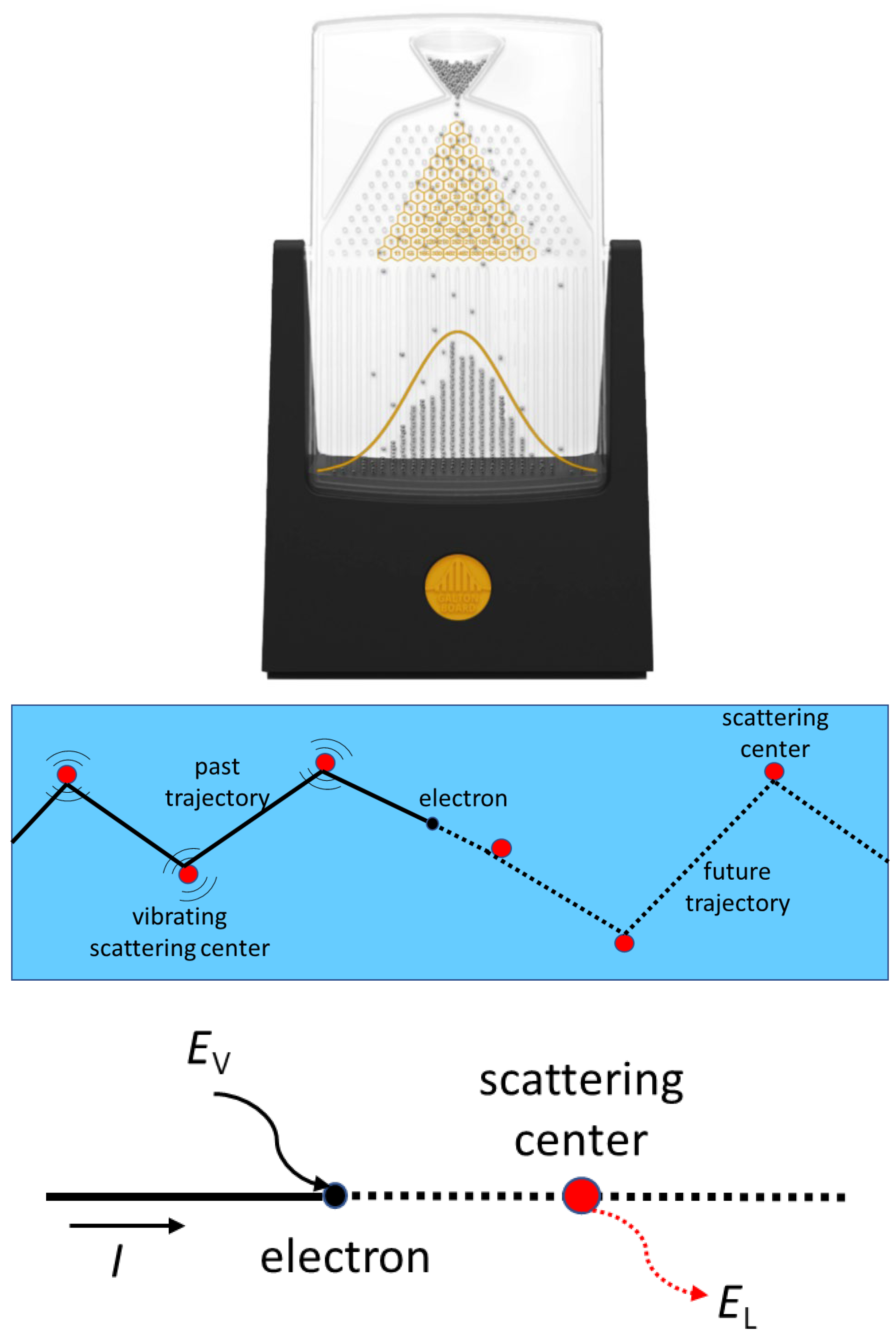
Figure 2.
Schematic flow diagram of the simulation processes.
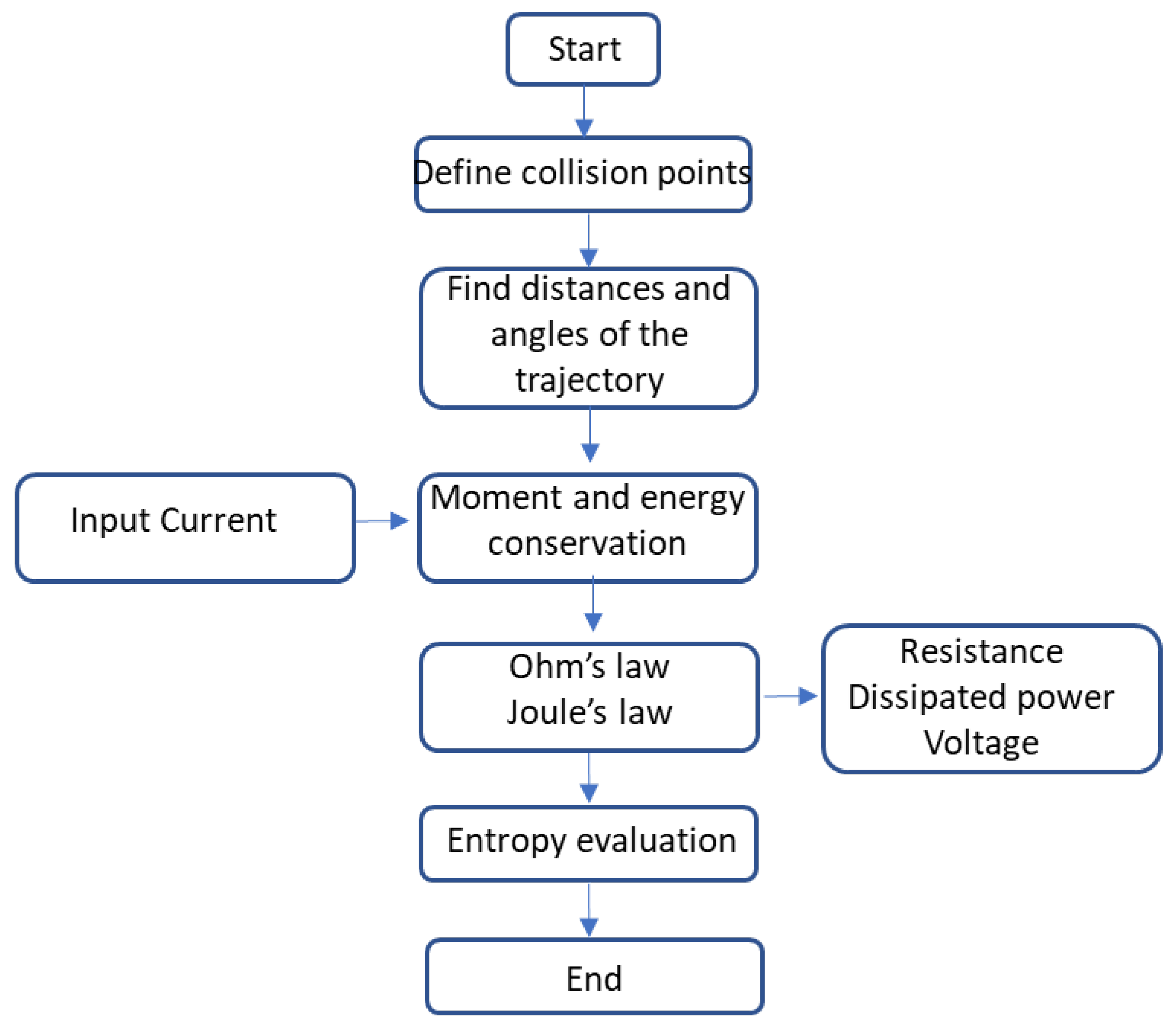
Figure 5.
Relationship between distance between collision centres and statistical entropy, Ss. The variance of the distribution is proportional to the distance σ= 6.88 d + 4.90 (correlation factor r=0.999). When averaged per unit length, the variation becomes constant.
Figure 5.
Relationship between distance between collision centres and statistical entropy, Ss. The variance of the distribution is proportional to the distance σ= 6.88 d + 4.90 (correlation factor r=0.999). When averaged per unit length, the variation becomes constant.
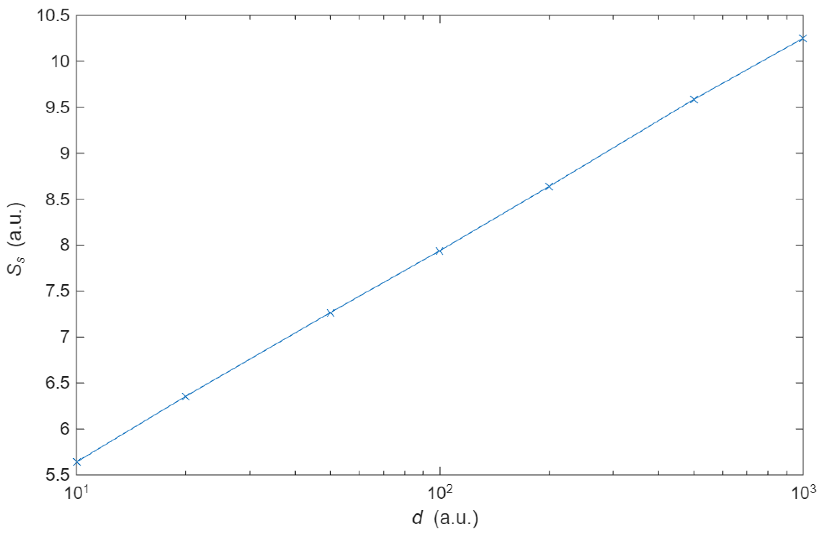
Figure 6.
– Digitalization of the trajectory by considering the probabilities of the electron moving up and down. The shorter dT path correspond to the maximum trajectory entropy. The longest path dT correspond to the minimum trajectory entropy.
Figure 6.
– Digitalization of the trajectory by considering the probabilities of the electron moving up and down. The shorter dT path correspond to the maximum trajectory entropy. The longest path dT correspond to the minimum trajectory entropy.
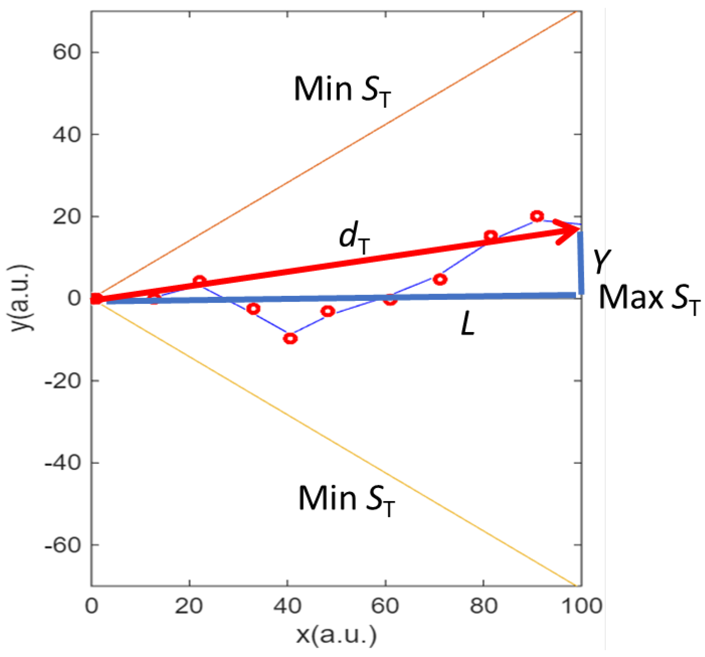
Figure 7.
Relationship between thermal entropy and configurational energy. The dots are obtained from simulations with 5000 electrons, 50 collisions and distances d from 10 to 1000 (The number labels distinguish the distance between scattering centres). The data fit a quadratic curve (in red), proving the causal relationship between the structure of the scattering centres and the energy dissipation.
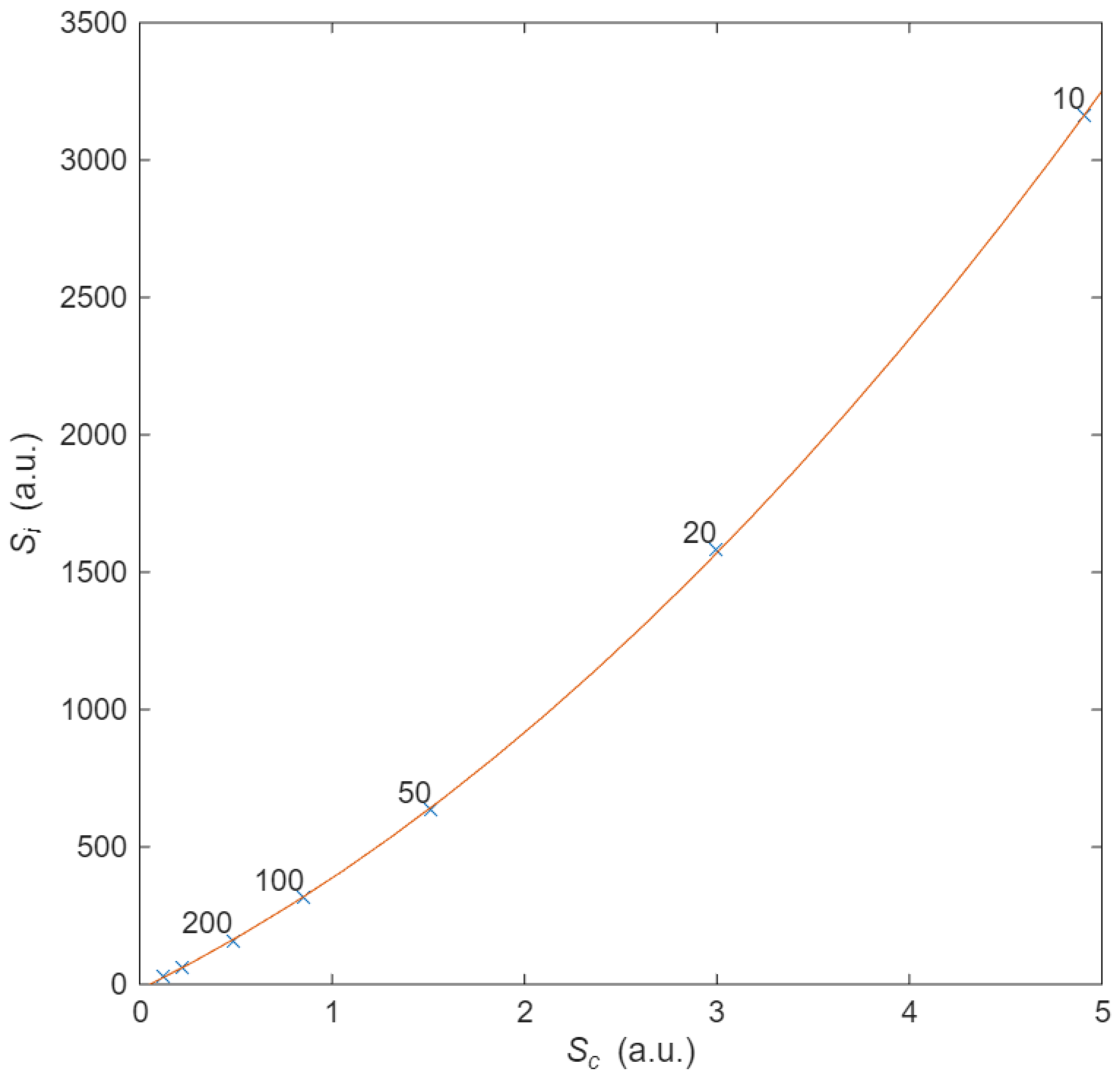

Table 1.
Different models for electron transport in solid conductors. In (1), I is the current, V the voltage and R the resistor. In 2, ρ is the resistivity, L the length and S the area, in (3), m* is the effective mass of the electrons, n the density of electrons, e the electrical charge of the electron and τ the relaxation time. In (4), g is the distribution that describes the gas of electrons, v the velocity, t ,r and k the time, position and moment of the electron.
| Model | Pros | Cons | |
|---|---|---|---|
| Ohm’s law (Classical) |
I=V/R (1) |
Simple to use. Experimentally available |
No information about material |
| Geometry (Classical) |
R=ρ L/S (2) | The constant is assigned to the material | ρ has to be found experimentally |
| Drude (semiclassical) |
(3) | ρ is inferred from intrinsic constants of the material. | different definitions of τ in literature has to be measured experimentally |
| Solid State (quantum) |
(4) | Solution of the quantum mechanics | Based on deterministic differential equations |
Disclaimer/Publisher’s Note: The statements, opinions and data contained in all publications are solely those of the individual author(s) and contributor(s) and not of MDPI and/or the editor(s). MDPI and/or the editor(s) disclaim responsibility for any injury to people or property resulting from any ideas, methods, instructions or products referred to in the content. |
© 2025 by the authors. Licensee MDPI, Basel, Switzerland. This article is an open access article distributed under the terms and conditions of the Creative Commons Attribution (CC BY) license (http://creativecommons.org/licenses/by/4.0/).
Copyright: This open access article is published under a Creative Commons CC BY 4.0 license, which permit the free download, distribution, and reuse, provided that the author and preprint are cited in any reuse.


