
Submitted:
02 September 2025
Posted:
03 September 2025
You are already at the latest version
Abstract
Thermal imaging is increasingly applied in remote sensing to identify material degradation, monitor structural integrity, and support energy diagnostics. However, its broader adoption is limited by the low spatial resolution of thermal sensors compared to RGB cameras. This study proposes a modular pipeline to generate thermally enriched 3D point clouds by fusing RGB and thermal imagery acquired simultaneously with a dual sensor unmanned aerial vehicle system. The methodology includes geometric calibration of both cameras, undistortion of images, cross-spectral feature matching, and projection of radiometric data onto the photogrammetric model (accepting a certain approximation) through a computed homography. Thermal values are extracted using a custom parser and assigned to 3D points based on visibility masks and interpolation strategies. Among twelve evaluated matching algorithms, LightGlue yielded the most accurate results. The system achieved subpixel reprojection errors and low temperature deviation from ground-truth data. A case study on photovoltaic panels demonstrates the method’s capability to identify surface anomalies and map thermal patterns with high spatial detail. Developed entirely in Python, the workflow can be integrated into Agisoft Metashape or adapted to other software. The proposed approach enables cost-effective, high-resolution thermal mapping and holds potential for civil engineering, cultural heritage conservation, and environmental monitoring applications.
Keywords:
thermal photogrammetry
; two-view geometry
; image fusion
; planar homography
; feature matching
1. Introduction
In the context of advances in intelligent techniques applied to the conservation of architectural heritage, three-dimensional digital documentation and multispectral analysis of historic buildings have gained a central role. The convergence of 3D modelling, artificial intelligence (AI), multi-view photogrammetry, and thermal or multispectral sensing is reshaping the way deterioration processes in heritage assets are detected, interpreted, and managed. This research addresses the integration of quantitative thermal data into high-resolution photogrammetric models as an accessible tool for non-destructive structural diagnosis and multi-scale documentation.
Fusing geometric and thermal domains within a three-dimensional framework is an ambitious yet highly valuable goal. 3D models generated through photogrammetry can accurately capture the shape and texture of heritage structures, enabling morphological analysis, the creation of digital twins, and longitudinal monitoring. In parallel, infrared thermography (IR) is widely recognised as a non-invasive technique to detect moisture ingress, delamination, insulation loss, or concealed defects. By combining these spatial and thermal domains, it becomes possible to localise thermal anomalies in a 3D spatial context, thereby improving both interpretability and interdisciplinary communication [1,2].
Nonetheless, this integration is not without significant technical challenges. One of the most critical is the inherently low spatial resolution of thermal sensors compared to RGB optical cameras. While visible-light cameras can achieve resolutions of 48MP or more, thermal cameras typically operate at 160×120 to 640×512 pixels. This disparity makes fine architectural details, such as hairline cracks, material joints, or ornamental features, invisible or blended in the thermal field. As a result, models generated solely from thermal imagery are often too sparse or inaccurate for meaningful 3D analysis [3]. Moreover, differences in perspective, distortion, and field of view between optical systems hinder direct registration and often prevent automatic integration of thermal data within standard photogrammetric workflows.
Thermal resolution thus becomes a bottleneck not only for building 3D thermal models, but also for radiometric interpretation of critical details. This challenge is magnified in complex architectural scenarios where surfaces are irregular, heights vary, and access is limited. In such contexts, traditional overlay techniques, based on planar homographies or manual registration, may prove insufficient or introduce systematic errors. Additionally, many existing solutions depend on specialised hardware, such as active thermal scanners, hardware-calibrated cameras, or proprietary systems with non-programmable pipelines, which restricts their applicability in real-world, low-budget settings [4,5].
Various approaches have been proposed to address this problem from different angles. Some methods map thermal images as textures onto pre-existing photogrammetric models, using planar transformations (homographies) between pre-calibrated optical systems [6]. While effective in planar scenes or constant-height contexts such as façades or flat roofs, this strategy falters in complex environments. Other authors have embedded thermal cameras directly into Structure-from-Motion (SfM) workflows, treating them as additional nodes in the reconstruction network, although performance is often constrained by the low number of keypoints detected in thermal imagery. More recently, hybrid workflows have emerged combining RGB reconstruction, multi-sensor calibration, and per-camera thermal projection to produce 3D thermotextured models [1,7]. Although technically sound, such approaches often involve intensive manual processing, proprietary software, or image-by-image adjustments, thus limiting their scalability and reproducibility.
With the advent of computer vision and deep learning, a new generation of algorithms has enabled robust matching between images, even across spectral domains. Models such as LightGlue, SuperGlue, and LoFTR have improved correspondence matching in optical systems, enhancing the estimation of homographies and relative poses [8,9,10]. In parallel, AI has been applied to classify thermal patterns in historical buildings, detecting moisture or degradation zones without manual supervision [11]. However, these advances have not yet been fully translated into reproducible workflows that programmatically and accurately generate 3D thermal models. A methodological gap remains between algorithmic potential and its practical application in heritage documentation and diagnostics.
This paper introduces a high-resolution 3D thermal mapping methodology, based on a reproducible, programmable, and low-cost pipeline. A dual-sensor acquisition system (RGB + thermal), mounted on a UAV or handheld platform, is used to capture data. A complete geometric calibration is performed, estimating intrinsic parameters of the cameras. This operation is based on a chessboard-style target visible in both spectral domains thanks to an evenly heated surface with infrared lamps. A precise point correspondence is obtained by leveraging machine learning and computer vision techniques to compute a single homography between imaging systems. The resulting approximated transformation enables the correlation of thermal coordinates onto the RGB images. Under controlled acquisition and co-mounted sensors, this strategy drastically reduces processing complexity without compromising spatial accuracy, as demonstrated in prior work [12].
Radiometric data is extracted using the manufacturer’s SDK (Software Development Kit). A dense point cloud is generated from RGB images using multi-image photogrammetry. After the RGB point cloud is reconstructed, visibility information is used to determine which thermal images observe each 3D point. Radiometric data is spatially interpolated before being assigned to each point. Consequently, all the elements of the cloud are enriched with a physical temperature value, moving beyond conventional false-colour representations or relative scales. The process is implemented in Python, integrating computer vision libraries and the Agisoft Metashape API (Application Programming Interface). Its automation ensures reproducibility and facilitates adaptation to different contexts or optical systems, including potential integration into Heritage Building Information Modelling (HBIM) platforms, energy analysis tools, or long-term monitoring frameworks.
The proposed system offers multiple operational advantages:
- it leverages the geometric detail of RGB reconstruction to compensate for low thermal resolution;
- it enables the inclusion of radiometrically accurate thermal data in 3D models;
- it avoids per-image registration, thus reducing processing time and cumulative errors;
- it is compatible with existing heritage workflows due to its integration into widely used software.
Moreover, the pipeline could be extended to multispectral sensors or integrated with deep learning techniques for automatic anomaly detection or thermal segmentation.
Applications of this type of enriched 3D thermal model are numerous: from precisely locating energy losses in historic building envelopes, to identifying structural pathologies not visible from the exterior, to tracking damage progression over time. It can also support advanced documentation of archaeological sites, energy efficiency assessment in heritage assets, or thermal mapping of climate-vulnerable structures.
This paper is structured as follows: Section 2 presents the objectives of the proposed pipeline; Section 3 reviews related work addressing similar challenges; Section 4 describes the acquisition system, optical system calibration, and thermal fusion strategy; Section 5 details the step-by-step methodology for building and enriching the point cloud; Section 6 presents a case study, including the results, quantitative analysis, and 3D visualisation of thermal anomalies; Section 7 discusses the results in relation to prior approaches and highlights the method’s limitations across various geometric scenarios; finally, Section 8 and Section 9 summarise the main contributions and proposes future research directions, including integration with hyperspectral sensors, neural architectures, and real-time embedded processing.
2. Goals
The general objective of this work is to develop and validate a reproducible methodology for generating high-resolution three-dimensional thermal models using dual-sensor acquisition systems (RGB + thermal), with applications in heritage documentation, structural monitoring, and non-destructive analysis. The proposed approach focuses on integrating radiometrically calibrated thermal information into dense point clouds obtained through multi-view photogrammetry, ensuring accurate, efficient, and scalable projection.
To achieve this general objective, the following specific goals are pursued:
- design a geometric calibration methodology, including all the intrinsic parameters for dual RGB–thermal optical systems. This stage involves validating calibration targets visible in both spectral domains and computing camera parameters, preparatory to the subsequent correlation between RGB and thermal images;
- identify an efficient algorithm for computing the homography between the thermal and RGB systems comparing the performance of various feature matching algorithms. The evaluation considers feature detection and correspondence methods such as DUSt3R [13], MASt3R [14], EfficientLoFTR [10], XoFTR [15], LiftFeat [16], RDD [17], LightGlue [9], DeDoDe [18,19], GIM [20], RoMa [21], OmnieGlue [22], and SuperGlue [8], assessing their robustness and accuracy under real-world acquisition conditions.
- implement an automated and programmable workflow, based on Python and the Agisoft Metashape API, that enables the fusion of thermal data into the point cloud generated from RGB imagery. This pipeline must be adaptable to different capture scenarios and facilitate integration into digital documentation processes.
- evaluate the accuracy and consistency of the resulting thermal model, considering both the spatial projection quality and the radiometric fidelity of the assigned thermal values. This includes analysing the mean absolute deviation against reference data and the procedural stability across varying configurations.
By fulfilling these objectives, the study seeks to contribute to the development of accessible, accurate, and reproducible solutions for enriched 3D thermal modelling, thereby expanding the reach of intelligent technologies applied to the conservation of the built heritage.
3. Related Works
The study of methods for generating thermal point clouds and integrating spectral data into photogrammetric workflows has received increasing attention over the past decade. This section reviews previous approaches related to four core aspects of the present research: 3D reconstruction from thermal images, optical system calibration, fusion techniques between thermal and RGB imagery, and feature matching algorithms applied across different spectral domains, particularly between RGB and thermal images.
3.1. Photogrammetric Point Cloud Generation from Thermal Imagery
Three-dimensional reconstruction based exclusively on thermal imagery has been explored primarily in energy inspection and structural monitoring applications, both in architecture and civil engineering. In these contexts, thermography is used to reveal surface anomalies related to heat loss, moisture ingress, or insulation defects [2]. However, generating dense point clouds from thermal images faces significant limitations, mainly due to the low spatial resolution of thermal cameras and the poor detectability of keypoints in such imagery.
It is possible to construct 3D thermal models using SfM and Multi-View Stereo (MVS) solely with thermal images, but the resulting models tend to be less detailed and noisier than those derived from RGB data [23]. To overcome these shortcomings, some researchers have developed hybrid techniques that combine photogrammetric reconstructions with post-hoc thermal texturing, or use base models obtained from RGB or LiDAR (Light Detection and Ranging) sensors onto which infrared radiometry is projected [1]. Other approaches employ monocular or stereo thermal reconstruction strategies using calibrated systems or high-sensitivity thermal sensors, although these typically involve higher costs [12].
In summary, although methods exist for generating point clouds from thermal imagery, their applicability is limited to scenarios with strong thermal texture, simple geometries, or high radiometric contrast. Most studies acknowledge the need to incorporate RGB sensors to improve the geometric fidelity of the resulting 3D model.
3.2. Optical System Calibration
The joint calibration of RGB and thermal sensors is a fundamental requirement for accurate data fusion in multispectral workflows. Various studies have proposed the use of custom-made calibration targets that are simultaneously visible in both the visible and infrared spectra [5]. These include heated checkerboards or passive panels with differential emissivity, enabling the estimation of intrinsic and extrinsic parameters and supporting full three-dimensional transformations, rotation and translation matrices.
Recent advances include the development of passive targets constructed with materials of contrasting emissivity, which improve thermal visibility under natural lighting conditions [24]. Other strategies involve active calibration devices with internal heating mechanisms that stabilise temperature throughout the capture sequence, thereby minimising thermal noise and improving repeatability [25].
Thermal image pre-processing also plays a key role. Applying contrast enhancement (e.g., histogram equalisation and CLAHE), intensity inversion, and adaptive thresholding using OTSU’s method enhances the detection of corners in thermal calibration targets when using computer vision techniques such as OpenCV [26,27].
3.3. Image Fusion Techniques
Fusing images from one sensor or diverse sensors, on the same or even with different spectral, optical, and geometric resolutions requires precise image registration strategies. Among the most used methods are projective transformations (homographies), direct registration based on intrinsic and extrinsic parameters (stereo calibration), and approaches based on automatic or manual correspondences.
The homography technique has been successfully applied in planar or controlled-depth scenes, such as façades or flat surfaces. This method assumes that all image points lie on a single plane or at a constant distance, which enables projection through a single transformation matrix [3]. In studies involving constant-altitude flights and co-mounted cameras, this assumption holds reasonably well, making homography an efficient and easily reproducible option. However, in scenes with significant parallax or complex geometry, this approach can introduce projection errors due to planarity assumptions, prompting the development of more robust methods such as direct projection, affecting both interior and exterior orientation.
Another class of data fusion techniques includes manual overlay registration, which, although still used in operational contexts, lacks reproducibility and scalability. These methods rely on the operator’s ability to manually align the thermal image onto the model, often resulting in inconsistent outcomes, particularly under uncontrolled acquisition conditions.
Recent advances in deep learning have opened new perspectives in multimodal registration. Unsupervised networks have been proposed to learn feature descriptors invariant to modality changes, significantly improving cross-spectral matching. For instance, contrastive learning frameworks trained on RGB images have demonstrated superior performance in handling spectral discrepancies, viewpoint changes, and scene complexity [32]. Similarly, domain adaptation techniques allow networks trained on RGB data to be generalised for thermal input, facilitating correspondence estimation across modalities without requiring exact spatial overlap [33].
In general, the most robust and accurate methods combine geometric calibration, optical distortion correction, and per-camera projection, allowing precise fusion of thermal data into high-resolution three-dimensional models.
3.4. Feature Matching Algorithms for Cross-Spectral Applications
Feature matching between RGB and thermal images represents one of the key challenges for multispectral integration within photogrammetric workflows. The spectral difference implies that many traditional descriptors, such as SIFT (Scale-Invariant Feature Transform), SURF (Speeded Up Robust Feature), ORB (Orientated FAST and Robust BRIEF), are unable to find reliable correspondences between images captured at different wavelengths. This limitation has led to the development of specialised algorithms, some based on deep learning, that can identify common points even when the visual content appears significantly different.
In this study, we conduct a comparative analysis of several matching algorithms that have demonstrated effectiveness in RGB context: DUSt3R, MASt3R, EfficientLoFTR, XoFTR, LiftFeat, RDD, LightGlue, DeDoDe, GIM, RoMa, OmniGlue and SuperGlue. Each of these methods is grounded in different architectural principles. Some, such as EfficientLoFTR and XoFTR, employ transformer-based architectures to model global spatial relationships, while others, like LightGlue and SuperGlue, rely on hybrid architectures that combine convolutional descriptors with attention modules [8,9,34].
DUSt3R and MASt3R integrate multi-level feature fusion and refinement mechanisms, making them suitable for low-overlap image pairs. LiftFeat and RDD, on the other hand, focus on robust keypoint extraction through supervised learning and have shown strong performance under adverse conditions. Although the use of these techniques in thermal–RGB contexts remains experimental, preliminary results are promising, particularly when combined with accurate calibration of the cameras.
The algorithms analysed not only improve RGB-thermal correlation, but also serve as key enablers for extending traditional photogrammetric pipelines into the multispectral domain, allowing for more automated and accurate workflows in heritage documentation projects.
3.5. Limitations and Gaps
Despite recent advances in 3D reconstruction techniques and multispectral data fusion, the specialised literature still presents several limitations that justify the need for new, accessible, and reproducible methodological proposals.
Firstly, methods that use thermal imagery for direct point cloud generation remain strongly constrained by the resolution and quality of infrared sensors. Even under high thermal contrast conditions, dense reconstruction based solely on thermal images typically yields sparse results, with low point density and a loss of geometric detail that is crucial for heritage analysis. This limits their practical applicability and often necessitates the use of additional sensors.
Secondly, although various approaches exist for correlating and fusing thermal imagery with RGB models, most of them suffer from at least one of the following shortcomings:
- reliance on proprietary, non-programmable tools;
- the need for manual registration steps, which lack reproducibility;
- use of homographies without prior calibration, which can lead to significant errors in scenes with parallax or irregular geometry.
- rigorous quantitative validation of the spatial and thermal accuracy of the resulting fusion.
Thirdly, the latest matching algorithms have shown strong potential, but their adoption in operational workflows remains limited. While some have been applied in registration or reconstruction tasks, systematic evaluations comparing their performance in RGB-thermal contexts under real capture conditions are still rare. Likewise, integrated workflows that combine matching, calibration, projection, and point cloud enrichment into a single programmable solution are seldom reported.
Finally, a significant methodological gap persists regarding the automation and standardisation of these processes. Existing solutions often require high levels of manual intervention or lack scalability, making them difficult to adopt in heritage workflows, where efficiency, traceability, and precision are required under technically constrained environments.
This landscape highlights the need for an approach that combines the geometric accuracy of RGB models, the calibrated radiometric information from thermal sensors, and the power of modern matching algorithms within a reproducible, validated, and adaptable workflow suited to different capture and analysis scenarios.
4. System Overview
The implementation of the proposed workflow requires a platform capable of capturing RGB and thermal images simultaneously, as well as a processing environment that integrates photogrammetry, computer vision, and programming tools. This section describes the data acquisition system, its main components, and the software tools used for automated processing. Figure 1 provides a schematic overview of the complete system, from field acquisition to the generation of the enriched thermal point cloud.
4.1. Dual-Sensor Platform
For this study, a DJI Mavic 3T drone was used, which features an integrated payload consisting of an RGB camera and a thermal camera. This system was selected because it allows for the simultaneous capture of both image types, reducing temporal offset between optical systems and minimising registration errors. Furthermore, it enables automated flight missions through precise trajectory planning over the area of interest, ensuring homogeneous and controlled coverage.
The technical specifications of both systems are presented in Table 1, including key characteristics such as effective resolution, lens type, field of view (FOV), and thermal sensitivity (NETD). These properties directly influence data quality and the accuracy of thermal fusion.
It is important to note that this approach is not limited exclusively to UAV platforms. The workflow can be adapted to systems mounted on tripods, masts, or handheld rigs, provided that their calibration is performed and the correlation between the dual sensor system of the frames is analysed. Nevertheless, the use of drones offers significant operational advantages, such as the ability to cover large areas automatically and to capture scenes from consistent angles and altitudes with a very small distance between the two optical systems, which facilitates the application of a single homography.
During the capture campaigns, a specific operational limitation of the DJI Mavic 3T was observed: if the shooting interval is equal to or less than 2 seconds, the system automatically reduces the resolution of the RGB sensor. This behaviour is related to the internal management of the sensor and the prevention of saturation artefacts. Therefore, for those wishing to replicate this methodology, it is recommended to plan flight missions with appropriate intervals between image captures. Despite this limitation, the system remains fully scalable and applicable to any dual-sensor platform that enables synchronisation and proper geometric control.
4.2. Software Environment
The processing of the captured data was carried out in an environment composed of tools widely recognised in the fields of photogrammetry and computer vision. Agisoft Metashape Professional was selected as the photogrammetric reconstruction engine due to its flexibility, accuracy, and compatibility with Python scripting. This last feature was particularly important, as it allowed the integration of the pipeline’s various modules within a single environment, facilitating the automation of the entire reconstruction and enrichment workflow.
Custom Python scripts were developed to automate key stages of the proposed pipeline, including sensor calibration, image undistortion, cross-spectral feature matching, homography computation, thermal data extraction, point cloud projection export, and thermal enrichment. These stages were integrated into Agisoft Metashape through its API, enabling structured access to camera parameters, image geometry, and spatial relationships, and ensuring reproducibility across datasets.
Python was chosen as the primary programming language for its seamless integration with computer vision and machine learning libraries. Specifically, OpenCV was used for image preprocessing, pattern detection, and geometric calculations; NumPy for efficient matrix handling; PyTorch for executing neural network-based matching models; and the DJI thermal SDK for extracting radiometrically calibrated values from the original image files.
The versions of the software and libraries used are listed in Table 2, to ensure reproducibility of the experiments and to facilitate the replication of the workflow in other environments.
This modular architecture enables future extensions to other sensors, capture formats, or specialised libraries, consolidating its value as an adaptable tool for multispectral heritage documentation projects.
5. Methodology
This section outlines the proposed methodology for generating a thermally enriched three-dimensional point cloud using a dual-sensor acquisition system. The workflow is structured into seven consecutive stages that enable, in an automated and reproducible manner, the capture of data, reconstruction of 3D geometry, extraction of calibrated thermal information, and its projection onto the 3D model. Each step was designed to minimise manual intervention and to ensure traceability between the captured images, camera parameters, and the thermal values assigned to each point. The following subsections describe each of these stages in detail.
5.1. Optical System Calibration
The first step of the proposed workflow consists of the geometric calibration of the RGB and thermal sensors, with the aim of correcting lens-induced distortions and estimating the intrinsic parameters required for the subsequent stages of image undistortion, spectral registration, and thermal data fusion. This step is critical to ensure accurate correspondence between RGB and thermal images, and to guarantee that thermal information can be coherently projected onto three-dimensional models generated via photogrammetry.
The need for multispectral calibration has been widely discussed in the literature. To achieve precise fusion across different spectral domains, it is essential to have well-defined intrinsic parameters for each optical system, and these parameters must be derived from patterns visible in both spectra [5]. In this context, several authors have proposed the use of heated checkerboards or materials with differential emissivity as practical solutions for thermal calibration targets [35,36].
In this work, a calibration pattern composed of black and white squares arranged as a 9×6 inner-corner checkerboard, with square cells of 40 mm, was designed. The pattern was printed on a rigid surface and placed on a flat base in a controlled temperature environment. It was heated using an infrared lamp, producing sufficient thermal contrast to make it visible in both the RGB and thermal domains. This strategy, recommended in prior cross-calibration studies [37], enabled detection of the same pattern in both modalities without the need for special sensors or active markers.
Image acquisition was performed using the DJI Mavic 3T UAV system, keeping the pattern centred within the frame and at a fixed distance from the sensors. Multiple photographs were taken from different perspectives to ensure sufficient coverage in terms of orientation and angle of view [38], following the recommendations of the pinhole camera model implemented in OpenCV. In the case of the thermal camera, it was necessary to invert the grayscale levels of the image, as heating reverses the expected contrast: black squares tend to absorb more radiation and appear hotter (and therefore brighter), while white squares reflect more and remain cooler.
Once the images were loaded into Agisoft Metashape within a single chunk configured as a Multi-Camera System, the software automatically identified the RGB–Thermal image pairs, assigning the sensors based on import order and dataset structure. The user can access the first step of the workflow through the Metashape interface by navigating to Scripts, 3D Thermal Mapping, STEP 1 - Calibrate Sensors, which opens an interactive window allowing confirmation of the primary (RGB) and secondary (Thermal) cameras, as well as the definition of the calibration pattern dimensions. By default, a 9×6 checkerboard with 40 mm square cells is used, although these parameters can be adjusted depending on the experimental setup. The system automatically stores the calibration results within the active project. Agisoft Metashape allows the export of the intrinsic matrices and distortion coefficients to external files for further use or independent validation.
Prior to the calibration computation, specific preprocessing techniques were applied to maximise pattern detectability. In RGB images, contrast normalisation and local adaptive histogram equalisation (CLAHE) were applied, while thermal images underwent greyscale inversion, automatic binary segmentation using Otsu’s method, and local thermal contrast enhancement. These operations proved particularly beneficial for improving pattern visibility in low-resolution thermal sensors.
The pattern detection process in each image involved a geometric analysis to locate the internal corners of the checkerboard and refine their positions using sub-pixel adjustment techniques. This was performed independently for both RGB and thermal images, ensuring high accuracy in both spectral domains. Once multiple pattern-image correspondences were identified across the dataset, individual calibration was carried out for each sensor, estimating the intrinsic matrix, optical distortion coefficients, and the rotation and translation vectors describing the pattern’s position relative to the camera. The entire procedure was implemented using OpenCV tools, which are widely validated for computer vision and multiview calibration tasks.
The results were integrated into the Metashape chunk to be used in subsequent stages of the pipeline. Additionally, Agisoft Metashape allows the export of the calibration parameters in .xml format for external traceability or for reuse in future projects using the same dual-sensor system.
The full calibration routine was automated through Python scripts, directly integrated into the Metashape API, enabling a repeatable, traceable, and replicable execution of the process, from image loading to parameter export. Figure 2 shows the flowchart corresponding to this procedure, as well as the Metashape interface used for its execution.
Reprojection errors were also computed individually per image, allowing for a quantitative assessment of the geometric calibration quality and enabling the selection of the most accurate views for the following stages of the workflow. When both cameras successfully detected the pattern in each capture, a joint calibration was performed, generating a stereoscopic configuration that includes the intrinsic parameters of each sensor and their relative spatial relationship. Figure 3 illustrates the results of this process, showing the original image of each sensor and the detected pattern in both modalities.
Figure 3 illustrates the results of the calibration step, showing the original and the detected chessboard on each pair.
5.2. Image Undistortion
Once both sensors have been calibrated and their respective intrinsic parameters, including lens distortion coefficients, have been obtained, the next step involves undistorting all captured images. This procedure aims to remove lens-induced deformations and produce images that conform to the pinhole projection model, which is essential for accurate geometric computations across views. In particular, prior undistortion improves both the numerical stability and accuracy of homography estimation, as point correspondences are established using distortion-free coordinates, a principle widely demonstrated in foundational computer vision studies [37].
The undistortion process is based directly on the camera matrices and distortion coefficients obtained in Section 5.1 (Sensor Calibration). These matrices enable the reconstruction of idealised image representations in which pixels correspond to linear projections on the image plane. The procedure was implemented through a Python script that automates the processing of RGB–Thermal image pairs. This script can be executed independently or integrated as an auxiliary module within Agisoft Metashape, allowing seamless incorporation into existing workflows.
Within the Metashape environment, this step can be initiated by navigating to Scripts, 3D Thermal Mapping, STEP 2 - Undistort Cameras. This action opens an interactive dialog that allows the user to select and launch the undistortion process. Internally, the script retrieves the calibration data stored in the current project and applies the transformation to each RGB–Thermal image pair. The resulting undistorted images are stored in a temporary chunk, which preserves the camera orientation and projection parameters, and can be directly used in the subsequent stage for homography computation. Figure 4 presents a flowchart of this process alongside its implementation within the Metashape environment.
The process leverages functions from the OpenCV library to generate undistorted images by correcting both radial and tangential distortion. Input and output resolutions are preserved to ensure consistency in scale and field of view.
Figure 5 presents visual examples comparing original and undistorted images from both the RGB and thermal channels. Notable improvements include the correction of peripheral curvature and the straightening of linear structures, which significantly enhance the reliability of feature matching in subsequent stages of the pipeline.
Although technical in nature, this step has a direct impact on the accuracy of downstream computations, particularly in multispectral contexts where geometric discrepancies between sensors tend to amplify registration errors. Ensuring that all images conform to the same projection model provides a reliable foundation for homography computation and the RGB-thermal registration described in the following section.
5.3. Cross-Spectral Feature Matching and Homography Computation
Precise registration between the RGB and thermal sensors is essential for the accurate transfer of radiometric information onto the 3D model. Since these sensors operate in distinct spectral domains, registering their respective images poses specific challenges, particularly in the detection and matching of keypoints. To address this issue, a two-stage strategy was implemented: an initial benchmarking phase involving feature matching algorithms, followed by the computation of a single homography matrix for the entire system.
During the evaluation phase, a representative set of ten RGB–Thermal image pairs, captured during the calibration process (see Section 5.1), was selected based on clear visibility of the calibration pattern in both channels. For each image pair, a series of manually annotated control points was recorded to serve as reference data.
Each image pair was processed using twelve state-of-the-art feature matching algorithms, selected for their proven performance in multispectral or multimodal contexts: DUSt3R, MASt3R, EfficientLoFTR, XoFTR, LiftFeat, RDD, LightGlue, DeDoDe, GIM, RoMa, OmniGlue and SuperGlue. These methods were assessed based on their ability to detect robust keypoints correspondences, generate sufficient match points, and enable stable projective transformation computation.
For each algorithm, a homography matrix was computed from the detected correspondences and applied to project thermal image points onto the RGB image plane. The projected points were then compared to the manually annotated control points, and the average Euclidean distance per image pair was calculated. A global mean error was subsequently computed across the ten pairs.
The algorithm yielding the lowest alignment error was selected as the optimal method and adopted as the default throughout the remainder of the pipeline, due to its robustness, accuracy, and efficiency under real-world acquisition conditions.
In the second stage, once the optimal method had been defined, it was applied to the newly acquired dataset. For each undistorted RGB-Thermal image pair, the selected algorithm was used to detect and match features, and a single homography matrix was computed between the sensors. This matrix encapsulates the geometric transformation between both sensors and is used in subsequent stages to project thermal data onto the 3D model.
The use of a single homography matrix, rather than one per image pair, is justified by the controlled acquisition conditions, fixed sensor mounting, consistent flight altitude, and the relatively planar nature of the observed scenes. These conditions make it possible to model the acquisition system as if all images were projected onto a shared planar surface, validating the use of a single global projective transformation [36]. This strategy significantly simplifies subsequent processing and avoids cumulative errors resulting from heterogeneous local estimations, as demonstrated in recent studies on multispectral fusion with co-mounted sensors [37].
To initiate the homography estimation step within Agisoft Metashape, the user must navigate to Scripts, 3D Thermal Mapping, STEP 3 - Calculate Homography. This action opens a dedicated dialog that guides the configuration and execution of the homography computation process. The interface allows the user to select the chunk containing the undistorted images generated in the previous step. By default, the script automatically selects the temporary chunk produced during the undistortion process; however, this can be manually modified to point to any compatible chunk within the current project.
Additionally, the user can choose the feature matching algorithm to be used for establishing point correspondences between the RGB and thermal images. By default, the system uses LightGlue, but alternative algorithms can be selected as needed. The dialog also exposes a set of algorithm-specific parameters that can be tuned to optimise detection thresholds, descriptor matching strategies, or filtering criteria, depending on the selected method. Figure 6 presents a flowchart outlining this procedure, along with a screenshot of the interface implemented in Metashape for user interaction.
A quantitative comparison of the accuracy achieved by each algorithm is presented in Section 7, along with an analysis of thermal accuracy and the final enriched 3D model.
5.4. Thermal Data Extraction
The next step in the pipeline involves extracting calibrated thermal information from each thermal image captured by the UAV system. This process aims to retrieve, for every pixel in the thermal image, a radiometrically corrected temperature value, adjusted according to ambient conditions and the physical properties of the observed surface.
To achieve this, a Python script was developed using DJI’s official SDK, with ExifTool employed as an auxiliary utility for accessing embedded image metadata. The script can be executed independently or integrated directly within the Agisoft Metashape environment, allowing seamless incorporation into photogrammetric workflows.
The procedure begins by reading the original thermal images, which are then processed through radiometric decoding using the parse_dirp2 function provided by the DJI SDK. This function outputs a temperature matrix with the same dimensions as the input image, where each cell represents the apparent surface temperature at the corresponding pixel. The resulting data is saved in compressed .npz format using the NumPy library, ensuring efficient storage and rapid access in downstream stages.
To improve thermal accuracy, the script incorporates several physical and environmental parameters that influence thermal data interpretation:
- ambient temperature, measured in situ during the field campaign.
- relative humidity, recorded under the same environmental conditions.
- material emissivity, defined according to standard reference tables.
- sensor-to-object distance, estimated from flight metadata.
These factors allow for correction of reflected temperature and compensate for systematic deviations due to external conditions, following established calibration principles for uncooled thermal sensors. The tool currently supports thermal images at 640×512 resolution and produces floating-point matrices ready for 3D mapping in the subsequent projection step.
To initiate this process within Metashape, the user must navigate to Scripts, 3D Thermal Mapping, STEP 4 - Extract Thermal Information. This action opens a dialog that allows the user to select the thermal sensor, which is automatically assigned by Metashape based on the project configuration but can be manually adjusted if necessary. The interface also enables the user to input the measured field conditions, including ambient temperature, relative humidity, material emissivity, and sensor-to-object distance, previously described in detail.
These values are then used to generate a temperature matrix for each thermal image, ensuring that the radiometric data are physically consistent with the acquisition context. The thermal outputs are stored and linked to the corresponding undistorted images, preparing them for integration with the RGB model in the final stage of the pipeline.
Figure 7 presents a flowchart describing this procedure, along with a screenshot of the script interface implemented in Agisoft Metashape.
This process ensures that each thermal image is associated with a matrix of physically meaningful data, prepared for integration with the RGB point cloud. In doing so, it enables precise projection of temperature values onto the reconstructed 3D model during the final stage of the workflow.
5.5. Photogrammetric Generation of High-Resolution RGB Point Cloud
Data acquisition for point cloud generation was carried out using a DJI Mavic 3T UAV platform, equipped with both RGB and thermal sensors. For the photogrammetric capture, the system’s wide-angle optical camera was used exclusively, as it offers higher spatial resolution compared to the telephoto camera, an essential factor for achieving a dense and accurate three-dimensional reconstruction. The selection of this camera maximises the geometric quality of the point cloud, leveraging its wider field of view, which is better suited to SfM and MVS reconstruction tasks.
The data acquisition flight was planned using an automated path divided into three grids: one for nadir images and two for oblique shots at 45 degrees, flown in orthogonal directions. To ensure robust coverage and reliable reconstruction, the RGB images were captured with 85% forward overlap and 80% side overlap. These values also provide good coverage for the thermal dataset, which features a narrower field of view compared to the RGB sensor. The flight speed was limited to 2 m/s to prevent an excessive shooting frequency that could overwhelm the RGB camera processor, potentially forcing it to reduce image resolution. This configuration ensures sufficient redundancy for multi-view triangulation and robust keypoint detection. Figure 8 shows the flight planning interface used during this phase.
Throughout the survey, a constant flight altitude was maintained to minimise parallax errors between cameras and to ensure that the homography conditions between image planes remained stable across the dataset.
This homogeneous acquisition condition is fundamental for later applying a single transformation matrix between sensors, without needing to recalculate it for each image pair. For this purpose, a technology based on a digital terrain model (DTM) with a resolution of 5 meters, obtained from LIDAR data, was used.
A Real-Time Kinematic (RTK) module was integrated into the drone in network mode to receive corrections from nearby permanent stations, thereby enhancing the positional accuracy of the captured images. This differential correction helps to reduce systematic geolocation errors and enhances geometric consistency among RGB images. While not essential to the proposed pipeline, the inclusion of accurate positioning supports more efficient photogrammetric orientation and can be relevant in applications requiring absolute georeferencing. To ensure maximum accuracy in the survey operations, 15 artificial checkerboard targets were uniformly distributed across the area of interest, ten of which were used as Ground Control Points (GCPs) and five as Check Points (CPs). The coordinates of these points were acquired using a GNSS antenna operating in network RTK (nRTK) mode. In accordance with the European INSPIRE directive (Technical Guidelines Annex I - D2.8.I.1), the geodetic reference system used for these operations was ETRS89, based on the GRS80 ellipsoid, which in Italy corresponds to the ETRF2000 realization (epoch 2008.0).
During the image acquisition, key environmental variables were also recorded for subsequent thermal processing. Ambient temperature and relative humidity were measured on site, as these parameters directly influence the calibration of thermal data. The estimated emissivity of the predominant material in the scene was also identified, based on reference tables, along with the average distance between the sensor and the object. These factors influence the apparent temperature measured by the thermal sensor. All this information was integrated into subsequent stages to refine radiometric interpretation and ensure that thermal values were physically meaningful.
The set of RGB images was processed using Agisoft Metashape Professional, following a standard photogrammetric workflow that included image orientation, structure optimisation, and dense image matching. The intrinsic and distortion matrices previously obtained during sensor calibration were incorporated into this process to correct optical deformations before reconstruction. Figure 9 presents a flowchart summarising the overall procedure followed during this stage.
Only the images from the wide-angle RGB camera were used in this stage. The resulting point cloud provides a high-resolution three-dimensional representation, which will later be enriched with thermal information. This reconstruction also allows for the extraction of camera projections needed to determine which images were observed at each point in the cloud, which is essential for thermal value assignment in the following steps. An example of the outcome of this stage is shown in Figure 10.
5.6. Exporting Point Cloud Reprojections
Following the generation of the dense point cloud described in the previous section, the next step involves exporting the image-space reprojections of each 3D point onto the set of calibrated RGB images. This process is essential for the subsequent thermal mapping stage, as it establishes a geometric correspondence between each 3D point in the model and its 2D reprojections in the original undistorted images.
To execute this step within Agisoft Metashape, the user must navigate to Scripts, 3D Thermal Mapping, STEP 6 - Export Reprojections. This opens a dedicated dialog where the user can choose whether to include all cameras in the export or restrict the output to a subset of selected cameras. Although the original dataset contains both RGB and thermal imagery, this step exclusively considers the RGB cameras, as they define the reference coordinate space for projection and colour mapping.
For each 3D point in the dense cloud, the script computes the corresponding (x,y) coordinates in each image where the point is visible. Additionally, the script records two quality metrics for each point-camera pair:
- the reprojection error, which quantifies the discrepancy between the observed and projected point positions, providing a measure of orientation reliability.
- the visibility state, which indicates whether the point is occluded or lies within the image frame and field of view.
These two metrics are retained for use in the next step of the pipeline, where they inform the selection of valid image observations for assigning thermal values to each 3D point.
The results are exported in a structured HDF5 file, saved automatically within the project directory. This file encodes the point IDs, projection coordinates, camera references, occlusion, and reprojection errors in an efficient format that supports fast access and large-scale processing.
Figure 11 presents a schematic of this step, showing the mapping between the 3D dense cloud and the 2D reprojections across selected RGB images, along with a screenshot of the interface in Metashape.
5.7. Thermal Enrichment of Point Cloud
The final stage of the proposed workflow consists of enriching the three-dimensional point cloud with calibrated thermal information, assigning a temperature value to each 3D point previously reconstructed via multi-view photogrammetry. This step synthesises and connects all the previous components: geometric calibration, image undistortion, spectral matching, and thermal data extraction.
The procedure was fully implemented in Python and designed to run either as a standalone application or embedded within the Agisoft Metashape environment via its scripting interface. This allows automation of the entire process, minimising manual errors and maintaining traceability between geometry and radiometric data. To launch the final stage of the workflow within Metashape, the user must navigate to Scripts, 3D Thermal Mapping, STEP 7 - Thermal Enrich Point Cloud. This action opens a simple dialog that allows the user to select the temperature value smoothing technique and initiate the thermal mapping process. No additional input is required at this stage, as all necessary data (undistorted imagery, thermal matrices, point reprojections, homography matrix, and camera parameters) have been prepared in previous steps. Figure 12 shows a flowchart of the implemented algorithm along with a partial view of its integration within the Agisoft interface.
The process relies on the camera projection data (calculated on the previous step, Section 5.6) stored in Agisoft Metashape, which makes it possible to determine, for each point in the cloud, which RGB images observed it and what its corresponding image-plane coordinates are. Using the RGB intrinsic and distortion matrices obtained during calibration (Section 5.1), the projected coordinates are corrected, yielding their exact position in the undistorted RGB image.
Next, the homography matrix between RGB and thermal (calculated in Section 5.3) is applied to project the RGB coordinates into the thermal image system. If the transformed point lies within the valid boundaries of the thermal image, it is first reprojected from the undistorted coordinate system back into the original form (using the camera’s intrinsic and distortion matrices calculated on Section 5.1), only then, the corresponding value in the calibrated temperature matrix (Section 5.4) is retrieved and assigned to the 3D point as an additional scalar attribute.
It is important to note that a single 3D point in the dense cloud may be projected onto multiple RGB images and, by extension, onto several corresponding thermal images via homography. To resolve this ambiguity and ensure the consistency of the thermal attribution, a visibility filtering and weighting strategy was implemented. This mechanism leverages the occlusion state and reprojection error values computed during the reprojection export stage (see Section 5.6) to determine whether a given point should be considered visible and geometrically reliable in a particular view. Reprojections flagged as occluded or exhibiting high reprojection error are automatically excluded from the fusion process to avoid erroneous temperature assignments.
For the remaining valid reprojections, where multiple views are available for a single point, a weighted aggregation of temperature values is performed. Each temperature is weighted based on the Euclidean distance between the image centre and the projected pixel coordinates (x,y). This approach favours pixels near the optical axis, where lens distortion is minimal and radiometric accuracy is typically higher. By applying this distance-based weighting, the process reduces peripheral artefacts and improves the spatial coherence of the thermal enrichment.
This strategy enables robust fusion of thermal data across multiple views, ensuring that each point in the cloud receives a reliable and physically meaningful temperature value, even in scenarios where redundancy or partial occlusion is present.
Furthermore, due to the difference in resolution between cameras, there may be significant divergence in the spatial density of pixels. That is, several RGB pixels might project onto the same thermal cell. To address this discrepancy, various smoothing and thermal interpolation strategies were evaluated, including:
- no interpolation, assigns the nearest thermal pixel value directly.
- linear interpolation, averages values from nearby pixels.
- bilinear interpolation, estimates the local plane using the four closest neighbours.
- trilinear interpolation, considers a constrained 3D neighbourhood.
- adaptive contour-preserving smoothing, applies a local mask that respects thermal discontinuities.
Each of these strategies offers advantages depending on the required level of accuracy and the regularity of the thermal pattern. In this work, bilinear interpolation was used by default, as it provides a good trade-off between radiometric fidelity and visual smoothness without excessive computational cost.
The outcome of this stage is a dense, thermally enriched point cloud in which each point contains not only RGB colour, 3D position, and normal vector, but also a scalar temperature value. This multispectral 3D model serves as a foundation for inspection tasks, structural pathology monitoring, or energy documentation of built heritage assets.
6. Case Study
To validate the proposed methodology, a first case study was carried out on a photovoltaic solar panel installation located on the university campus. This type of scenario is particularly suitable for thermal evaluation, as anomalies in the temperature distribution can reveal defective cells, efficiency losses, or failures in the heat dissipation system. Moreover, the flat, well-defined, and sun-exposed surfaces provide ideal geometric conditions to assess the effectiveness of the thermal–geometric fusion process.
The full workflow was executed, from flight planning to the generation of the enriched 3D model. The aerial survey was conducted under supervised weather conditions, using a constant distance from the ground of about 30 meters
During processing, the performance of the previously selected feature matching algorithm was verified, with robust registration observed between RGB–Thermal image pairs, even under moderate thermal contrast conditions. In one of the analysed scenes, precise correspondences were achieved, as illustrated in Figure 13, where matched points across spectral domains are shown using the adopted method.
To visually assess the accuracy of the computed homography, composite images were generated by superimposing the thermal image onto the undistorted RGB image. This type of visualisation, shown in Figure 14, enables the spatial alignment between structural edges (e.g., panel borders, cast shadows) and their associated thermal variations to be evaluated. The accurate contour matching confirms the effectiveness of the underlying geometric model.
Finally, thermal enrichment of the point cloud was performed. The results are presented in Figure 15, which shows, on the left, the dense RGB model reconstructed via photogrammetry and, on the right, the point cloud enriched with thermal information. In the latter, each 3D point is assigned a scalar value coded chromatically according to surface temperature. This multispectral 3D representation allows for high-fidelity visualisation of thermal distribution mapped onto the real-world geometry of the system.
The results obtained confirm the operational viability of the proposed approach. Spectral registration was accurate, temperature assignment was continuous and coherent, and the final model enables the identification of localised overheating zones. This capacity to represent thermal information directly on 3D models opens new possibilities in preventive diagnostics, energy monitoring, and multispectral digital modelling of infrastructure.
7. Results
This section presents the results obtained from the application of the proposed workflow, both during the calibration phase and in the subsequent case study. The results are presented through a combination of qualitative and quantitative observations, structured in accordance with each stage of the pipeline, from pattern detection to the final visualisation of the thermally enriched 3D model.
7.1. Pattern Detection and Image Undistortion
The first key stage involved detecting the calibration pattern within the captured RGB and thermal images. The dataset comprised 88 images, after applying domain-specific preprocessing to each spectral channel, the algorithm failed to detect the calibration pattern in only 2 RGB and 16 thermal images, therefore the chessboard was successfully detected in 72 image pairs (81.8 % of the total). This detection rate provided a sufficient number of image pairs to carry out the calibration of both sensors and proceed with the workflow.
7.2. Feature Matching Evaluation
During the evaluation phase of the feature matching algorithms, the twelve selected models were applied to a subset of ten RGB-Thermal pairs from the calibration dataset. For each case, the mean reprojection error was calculated, expressed as the Euclidean distance between the points projected by the homography and the manually defined control points.
Table 3 summarizes, for each algorithm, the proportion of initial matches retained after geometric verification (% matches) and the area under the cumulative reprojection error curve at tolerances of 1 px, 3 px and 5 px (AUC@1 px, AUC@3 px and AUC@5 px). % matches reflects the percentage of raw keypoint pairs that survive RANSAC, while each AUC metric measures the fraction of these surviving correspondences whose reprojection error falls within the given pixel threshold. As highlighted in bold, LightGlue retains 99.0 % of its matches, higher than SuperGlue’s 98.0 % and EfficientLoF’s 47.6 %, and achieves the best AUC scores at all three thresholds (18.2 % at 1 px, 65.1 % at 3 px and 79.0 % at 5 px). These results demonstrate that LightGlue consistently produces a greater proportion of highly accurate correspondences than its competitors.
Figure 16 shows visual examples of the feature matching process for three different algorithms (Dust3R, GIM-dmk and Mast3R), allowing comparison of the density and accuracy of the projected correspondences between RGB and IR domains.
Once the optimal algorithm was selected, the homography matrix between sensors was computed. The validation of this transformation can be observed in the visual compositions generated by overlaying thermal images onto their corresponding RGB images.
Figure 17 shows this result for a scene from the calibration environment, where a precise alignment of the chessboard edges is visible across both spectral domains. In contrast.
7.3. Radiometric Extraction
Thermal data extraction was performed on all thermal images in the dataset, generating a temperature matrix for each. These matrices contain physical values in degrees Celsius, corrected for emissivity, humidity, ambient temperature, and distance to the object. Although this process does not yield an inherently visual result, a region of interest was selected showing a portion of a solar panel, represented in matrix format in Figure 18, where colour encodes temperature and numerical values are overlaid.
7.4. Thermal Enriched 3D Model
Finally, the thermal data were integrated into the three-dimensional point cloud generated from the RGB images. The result was a multispectral model in which each point contains, in addition to colour and geometric information, a scalar temperature value.
Figure 19 illustrates a representative section of the thermally enriched 3D point cloud. Five points are highlighted with their corresponding temperature values, expressed as Scalar field. The graphic also includes one of the corresponding thermal images of that specific region and, in the upper-right corner, a cropped view indicating the region of interest used for analysis. It is also possible to distinguish areas with homogeneous temperatures and others with localized variations, possibly associated with defects or differences in solar exposure.
8. Discussion
The proposed approach has proven effective for integrating calibrated thermal information into high-resolution three-dimensional models without requiring specialized equipment or proprietary workflows. However, the process is not free from technical challenges, which merit discussion, as well as opportunities for future expansion and adaptation.
One of the main advantages of the proposed pipeline is its modularity and operational flexibility. All components were developed in Python using open-source libraries, allowing each module to be executed independently or integrated as an extension within existing photogrammetric software. In this study, the pipeline was embedded directly into Agisoft Metashape, leveraging its native scripting system. Nevertheless, it can be adapted to other platforms, as the required data (point clouds, camera projections, RGB/Thermal images) are compatible with any software adhering to common photogrammetric standards. This opens the door to integration in environments such as MicMac, COLMAP, or RealityCapture, or even with point clouds generated by active sensors like LiDAR.
Another relevant aspect concerns the generation of thermally visible patterns for sensor calibration. In this work, a chessboard-style target heated with an infrared lamp was used, but other valid configurations exist, such as circular patterns, Charuco boards, or active emitters for dark scenes. The pattern choice depends on the sensor used, its resolution, thermal range, and the ability to obtain sufficient contrast between cells. The literature shows that with appropriate preprocessing techniques, robust multispectral calibrations are possible even under challenging conditions.
For thermal data extraction, the DJI SDK was used alongside a custom Python script, compatible with a wide range of commercial cameras, including FLIR AX8, FLIR B60, FLIR E40, FLIR T640, DJI H20T, DJI XT2, DJI XTR, DJI XTS, Zenmuse XT S, DJI M2EA, H20N, M3T, M30T, M3TD, H30T, and Matrice 4. Nonetheless, this module can be easily replaced by another SDK or parser compatible with different thermal camera models or brands. The architecture of the system does not depend on the manufacturer, but rather on access to a calibrated radiometric map, making it highly extensible to new platforms.
Regarding feature matching algorithms, the pipeline was designed to remain agnostic to the specific method employed. In this study, twelve modern algorithms were evaluated, and the best-performing one was selected as the default. However, the architecture allows for the easy integration, evaluation, and use of new algorithms as they emerge from the computer vision community, without affecting the rest of the system.
Finally, it is important to highlight that one of the main challenges of this type of multispectral fusion is its sensitivity to geometric discrepancies between image captures. Despite the joint calibration and image undistortion, parallax (particularly in non-planar surfaces or those with significant depth) can introduce projection errors. This effect is worsened when there are variations in the distance between the sensors and the target, especially in geometrically irregular environments. To mitigate this, in our study the flight altitude was kept constant, and the analysis was limited to predominantly planar scenes, such as photovoltaic panels. However, in more complex contexts, it will be necessary to incorporate additional strategies such as local homography correction or 3D reprojection using depth maps.
9. Future Works
Although the proposed pipeline has proven effective for generating thermally enriched 3D models, several technical and conceptual aspects remain to be addressed and optimized in future work.
The integration of a thermally regulated element within the calibration scene. For instance, a controllable heating device, such as a resistive element with variable output, could be employed to maintain a fixed temperature. This would enhance the thermal contrast of the calibration pattern, particularly the checkerboard rectangles, thereby improving their detectability in the infrared spectrum. Such an approach could serve as a contrast adjustment mechanism during the training survey used to compute the intrinsic parameters of the thermal camera.
One of the main challenges identified is the presence of parallax in scenes with variable depth. This paper adopted the simplification of a global homography between sensors, which is valid under the assumption of planar scenes and constant distance between the camera and the target. However, in more complex contexts, this assumption no longer holds, leading to projection errors. A potential direction for future research involves estimating local homographies for each image pair or even for individual image regions. While this approach increases computational complexity, it can enhance geometric fidelity. Alternatively, using depth maps derived from the dense model would allow for more accurate thermal reprojection onto the 3D cloud, correcting parallax effects based on the actual geometry of the scene.
Another promising extension lies in the integration of multispectral sensors. Although this work focused specifically on RGB and thermal data, the pipeline is conceptually extensible to other spectral domains, such as near-infrared (NIR), red-edge, or even hyperspectral imagery. This would enable applications in precision agriculture, material moisture analysis, or biological stress detection, among others.
Furthermore, the modular architecture of the pipeline facilitates its adoption in real-time contexts, whether embedded on UAVs with onboard computing capabilities or on stationary systems for continuous monitoring. Achieving this would require additional optimization in terms of computational efficiency and parallelization, as well as the possible integration of neural networks for segmentation or cross-spectral image matching.
Finally, future work should explore the incorporation of supervised deep learning techniques to improve both homography estimation and thermal interpolation. Models trained specifically for cross-spectral transfer tasks could reduce matching errors and increase system robustness under uncontrolled conditions.
10. Conclusions
This work presents a modular and replicable processing pipeline for the generation of 3D point clouds enriched with thermal information, by combining RGB and thermal images captured simultaneously using a dual-sensor platform. The pipeline includes well-defined stages covering geometric calibration, image undistortion, cross-spectral feature matching, radiometric data extraction, and finally, thermal projection onto three-dimensional models.
Using open-source tools and Python-based scripts, the system was implemented within the Agisoft Metashape environment, although its architecture allows for adaptation to any compatible photogrammetric software or for standalone use. The case study applied to photovoltaic solar panels demonstrated the practical feasibility of the approach, both in terms of geometric accuracy and thermal continuity on the final 3D model.
Among the most relevant outcomes are the effectiveness of the selected matching algorithm, the accuracy of the thermal projection, and the ability to detect temperature patterns on complex geometries without the need for expensive fused sensors. Furthermore, limitations associated with parallax were addressed, and potential improvements were discussed, including the use of local homographies or depth maps.
Overall, this approach lays the groundwork for accessible high-resolution 3D thermal fusion, with potential applications in structural monitoring, energy inspection, heritage documentation, and precision agriculture. Its open and scalable design enables future extensions to other spectral domains, new sensor platforms, or real-time applications.
Author Contributions
Conceptualization, N.G. and A.d.F.; methodology, N.G. and A.d.F.; software, N.G.; validation, N.G., S.B. and A.d.F.; formal analysis, N.G. and A.d.F.; investigation, N.G., A.d.F and S.B.; resources, N.G. and A.dF.; data curation, N.G.; writing-original draft preparation, N.G. and A.d.F; writing-review and editing, N.G., S.B. and A.dF.; visualization, N.G.; supervision, A.d.F. and S.B.; project administration, A.d.F.; funding acquisition, S.B. All authors have read and agreed to the published version of the manuscript.
Funding
This research received no external funding.
Institutional Review Board Statement
Not applicable.
Informed Consent Statement
Not applicable.
Data Availability Statement
Not applicable.
Acknowledgments
The authors gratefully acknowledge the support provided by the University of Salerno, particularly the Modelli Laboratory of the Department of Civil Engineering, for supplying the UAV used in the data acquisition campaign and for providing the computing infrastructure necessary for the development and processing of the dataset.
Conflicts of Interest
The authors declare no conflict of interest.
Abbreviations
The following abbreviations are used in this manuscript:
| MDPI | Multidisciplinary Digital Publishing Institute |
| AI | Artificial Intelligence |
| IR | Infrared |
| UAV | Unmanned Aerial Vehicle |
| SfM | Structure from Motion |
| SDK | Software Development Kit |
| API | Application programming interface |
| HBIM | Heritage Building Information Modelling |
| MVS | Multi-View Stereo |
| LiDAR | Light Detection and Ranging |
| SIFT | Scale-Invariant Feature Transform |
| SURF | Speeded Up Robust Feature |
| ORB | Orientated FAST and Robust BRIEF |
| FOV | Field of View |
| NETD | Noise Equivalent Temperature Difference |
| RTK | Real-Time Kinematic |
| NIR | Near InfraRed |
References
- Patrucco, G.; Gómez, A.; Adineh, A.; Rahrig, M.; Lerma, J.L. 3D Data Fusion for Historical Analyses of Heritage Buildings Using Thermal Images: The Palacio de Colomina as a Case Study. Remote Sens. 2022, 14, 5699. [Google Scholar] [CrossRef]
- Sutherland, N.; Marsh, S.; Priestnall, G.; Bryan, P.; Mills, J. InfraRed Thermography and 3D-Data Fusion for Architectural Heritage: A Scoping Review. Remote Sens. 2023, 15, 2422. [Google Scholar] [CrossRef]
- Adamopoulos, E.; Volinia, M.; Girotto, M.; Rinaudo, F. Three-Dimensional Thermal Mapping from IRT Images for Rapid Architectural Heritage NDT. Buildings 2020, 10, 187. [Google Scholar] [CrossRef]
- Hou, Y.; Chen, M.; Volk, R.; Soibelman, L. Investigation on Performance of RGB Point Cloud and Thermal Information Data Fusion for 3D Building Thermal Map Modeling Using Aerial Images under Different Experimental Conditions. J. Build. Eng. 2022, 45, 103380. [Google Scholar] [CrossRef]
- ElSheikh, A.; Abu-Nabah, B.A.; Hamdan, M.O.; Tian, G.-Y. Infrared Camera Geometric Calibration: A Review and a Precise Thermal Radiation Checkerboard Target. Sensors 2023, 23, 3479. [Google Scholar] [CrossRef] [PubMed]
- Ramón, A.; Adán, A.; Javier Castilla, F. Thermal Point Clouds of Buildings: A Review. Energy Build. 2022, 274, 112425. [Google Scholar] [CrossRef]
- Adamopoulos, E.; Patrucco, G.; Volinia, M.; Girotto, M.; Rinaudo, F.; Tonolo, F.G.; Spanò, A. 3D Thermal Mapping of Architectural Heritage. In Proceedings of the Digital Heritage. Progress in Cultural Heritage: Documentation, Preservation, and Protection; Ioannides, M., Fink, E., Cantoni, L., Champion, E., Eds.; Springer International Publishing: Cham, 2021; pp. 26–37.
- Sarlin, P.-E.; DeTone, D.; Malisiewicz, T.; Rabinovich, A. SuperGlue: Learning Feature Matching with Graph Neural Networks 2020.
- Lindenberger, P.; Sarlin, P.-E.; Pollefeys, M. LightGlue: Local Feature Matching at Light Speed 2023.
- Wang, Y.; He, X.; Peng, S.; Tan, D.; Zhou, X. Efficient LoFTR: Semi-Dense Local Feature Matching with Sparse-Like Speed.; 2024; pp. 21666–21675.
- Alexakis, E.; Delegou, E.T.; Mavrepis, P.; Rifios, A.; Kyriazis, D.; Moropoulou, A. A Novel Application of Deep Learning Approach over IRT Images for the Automated Detection of Rising Damp on Historical Masonries. Case Stud. Constr. Mater. 2024, 20, e02889. [Google Scholar] [CrossRef]
- Piccinelli, N.; De Rossi, G.; Daffara, C.; Muradore, R. A Passive Stereo Calibration Technique for Visible-Thermal, Low-Resolution Imaging in Remote Sensing Applications. Measurement 2024, 231, 114647. [Google Scholar] [CrossRef]
- Wang, S.; Leroy, V.; Cabon, Y.; Chidlovskii, B.; Revaud, J. DUSt3R: Geometric 3D Vision Made Easy.; 2024; pp. 20697–20709.
- Leroy, V.; Cabon, Y.; Revaud, J. Grounding Image Matching in 3D with MASt3R. In Proceedings of the Computer Vision – ECCV 2024; Leonardis, A., Ricci, E., Roth, S., Russakovsky, O., Sattler, T., Varol, G., Eds.; Springer Nature Switzerland: Cham, 2025; pp. 71–91.
- Tuzcuoğlu, Ö.; Köksal, A.; Sofu, B.; Kalkan, S.; Alatan, A.A. XoFTR: Cross-Modal Feature Matching Transformer.; 2024; pp. 4275–4286.
- Liu, Y.; Lai, W.; Zhao, Z.; Xiong, Y.; Zhu, J.; Cheng, J.; Xu, Y. LiftFeat: 3D Geometry-Aware Local Feature Matching 2025.
- Chen, G.; Fu, T.; Chen, H.; Teng, W.; Xiao, H.; Zhao, Y. RDD: Robust Feature Detector and Descriptor Using Deformable Transformer.; 2025; pp. 6394–6403.
- Edstedt, J.; Bökman, G.; Wadenbäck, M.; Felsberg, M. DeDoDe: Detect, Don’t Describe - Describe, Don’t Detect for Local Feature Matching. In Proceedings of the 2024 International Conference on 3D Vision (3DV); March 2024; pp. 148–157.
- Edstedt, J.; Bökman, G.; Zhao, Z. DeDoDe v2: Analyzing and Improving the DeDoDe Keypoint Detector.; 2024; pp. 4245–4253.
- Shen, X.; Cai, Z.; Yin, W.; Müller, M.; Li, Z.; Wang, K.; Chen, X.; Wang, C. GIM: Learning Generalizable Image Matcher From Internet Videos 2024.
- Edstedt, J.; Sun, Q.; Bökman, G.; Wadenbäck, M.; Felsberg, M. RoMa: Robust Dense Feature Matching 2023.
- Jiang, H.; Karpur, A.; Cao, B.; Huang, Q.; Araujo, A. OmniGlue: Generalizable Feature Matching with Foundation Model Guidance 2024.
- Dlesk, A.; Vach, K.; Pavelka, K. Transformations in the Photogrammetric Co-Processing of Thermal Infrared Images and RGB Images. Sensors 2021, 21, 5061. [Google Scholar] [CrossRef] [PubMed]
- Kinnen, T.; Blut, C.; Effkemann, C.; Blankenbach, J. Thermal Reality Capturing with the Microsoft HoloLens 2 for Energy System Analysis. Energy Build. 2023, 288, 113020. [Google Scholar] [CrossRef]
- Roshan, M.C.; Isaksson, M.; Pranata, A. A Geometric Calibration Method for Thermal Cameras Using a ChArUco Board. Infrared Phys. Technol. 2024, 138, 105219. [Google Scholar] [CrossRef]
- Sher, B.A.; Xu, X.; Chen, G.; Feng, C. Marker-Based Extrinsic Calibration for Thermal-RGB Camera Pair with Different Calibration Board Materials. Int. Symp. Autom. Robot. Constr. ISARC Proc. 2023, 2023 Proceedings of the 40th ISARC, Chennai, India, 490–497. [CrossRef]
- Infrared Camera Geometric Calibration: A Review and a Precise Thermal Radiation Checkerboard Target. Available online: https://www.mdpi.com/1424-8220/23/7/3479 (accessed on 4 August 2025).
- Choinowski, A.; Dahlke, D.; Ernst, I.; Pless, S.; Rettig, I. AUTOMATIC CALIBRATION AND CO-REGISTRATION FOR A STEREO CAMERA SYSTEM AND A THERMAL IMAGING SENSOR USING A CHESSBOARD. Int. Arch. Photogramm. Remote Sens. Spat. Inf. Sci. 2019, XLII-2-W13, 1631–1635. [CrossRef]
- Calibration for 3D Reconstruction of Thermal Images | Request PDF. In Proceedings of the ResearchGate.
- Saponaro, P.; Sorensen, S.; Rhein, S.; Kambhamettu, C. Improving Calibration of Thermal Stereo Cameras Using Heated Calibration Board. In Proceedings of the 2015 IEEE International Conference on Image Processing (ICIP); September 2015; pp. 4718–4722.
- Chen, Y.; Huang, F.; Shi, F.; Liu, B.; Yu, H. Plane Chessboard-Based Calibration Method for a LWIR Ultra-Wide-Angle Camera. Appl. Opt. 2019, 58, 744–751. [Google Scholar] [CrossRef] [PubMed]
- Hong, M.; Lu, Y.; Ye, N.; Lin, C.; Zhao, Q.; Liu, S. Unsupervised Homography Estimation with Coplanarity-Aware GAN 2022.
- Zhang, J.; Wang, C.; Liu, S.; Jia, L.; Ye, N.; Wang, J.; Zhou, J.; Sun, J. Content-Aware Unsupervised Deep Homography Estimation 2020.
- Sarlin, P.-E.; Cadena, C.; Siegwart, R.; Dymczyk, M. From Coarse to Fine: Robust Hierarchical Localization at Large Scale 2019.
- Vidas, S.; Lakemond, R.; Denman, S.; Fookes, C.; Sridharan, S.; Wark, T. A Mask-Based Approach for the Geometric Calibration of Thermal-Infrared Cameras. IEEE Trans. Instrum. Meas. 2012, 61, 1625–1635. [Google Scholar] [CrossRef]
- Zhang, Z. Camera Calibration. In Computer Vision; Springer, Cham, 2021; pp. 130–131 ISBN 978-3-030-63416-2.
- Luhmann, T.; Piechel, J.; Roelfs, T. Geometric Calibration of Thermographic Cameras. In Thermal Infrared Remote Sensing: Sensors, Methods, Applications; Kuenzer, C., Dech, S., Eds.; Springer Netherlands: Dordrecht, 2013; pp. 27–42. ISBN 978-94-007-6639-6. [Google Scholar]
- Parrinello, S.; De Marco, R. Digital Strategies for Endangered Cultural Heritage. Forthcoming Interspecies: Handbook of Research on Strategies and Creative Interdisciplinarity for the Digitization and Safeguard of Endangered Heritage. PROSPETTIVE MULTIPLE: STUDI DI INGEGNERIA, ARCHITETTURA E ARTE,2023,pp 1-288.
Figure 1.
System overview and processing workflow for 3D thermal point cloud generation.
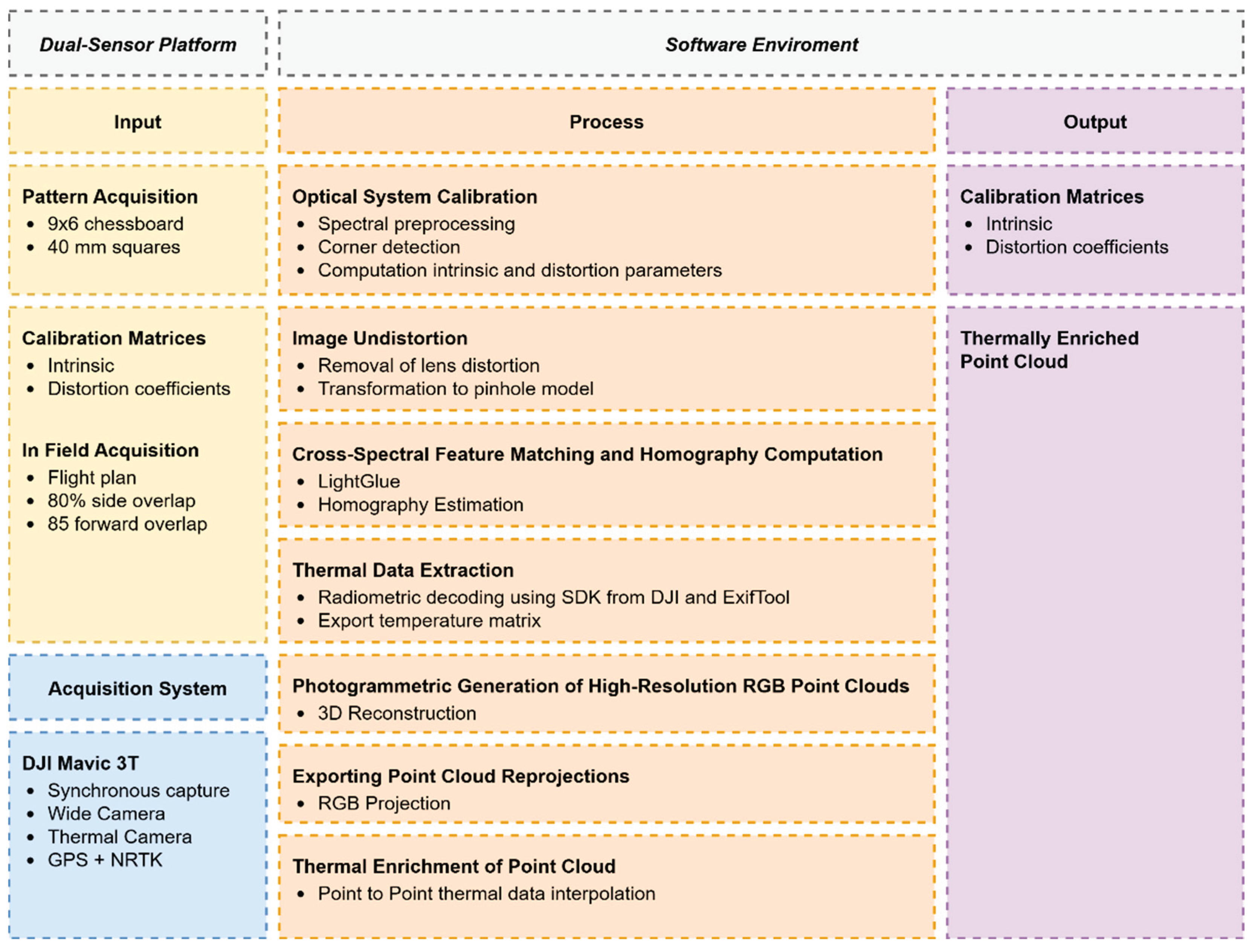
Figure 2.
Sensor calibration pipeline: (a) processing flowchart; (b) implementation in Agisoft Metashape.
Figure 2.
Sensor calibration pipeline: (a) processing flowchart; (b) implementation in Agisoft Metashape.
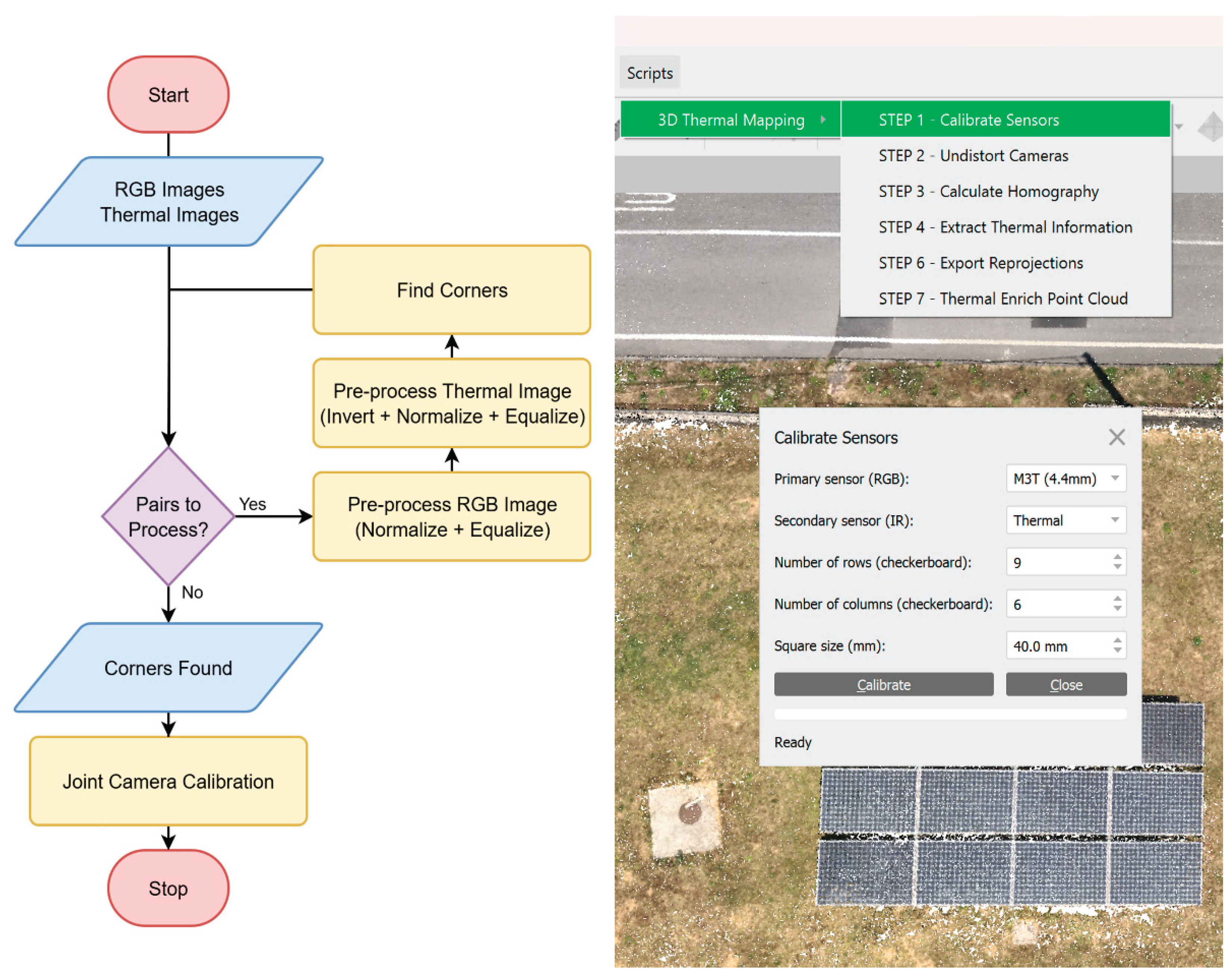
Figure 3.
Comparison of original and the chessboard found on a subset of 4 pairs (RGB on the left and thermal on the right).
Figure 3.
Comparison of original and the chessboard found on a subset of 4 pairs (RGB on the left and thermal on the right).
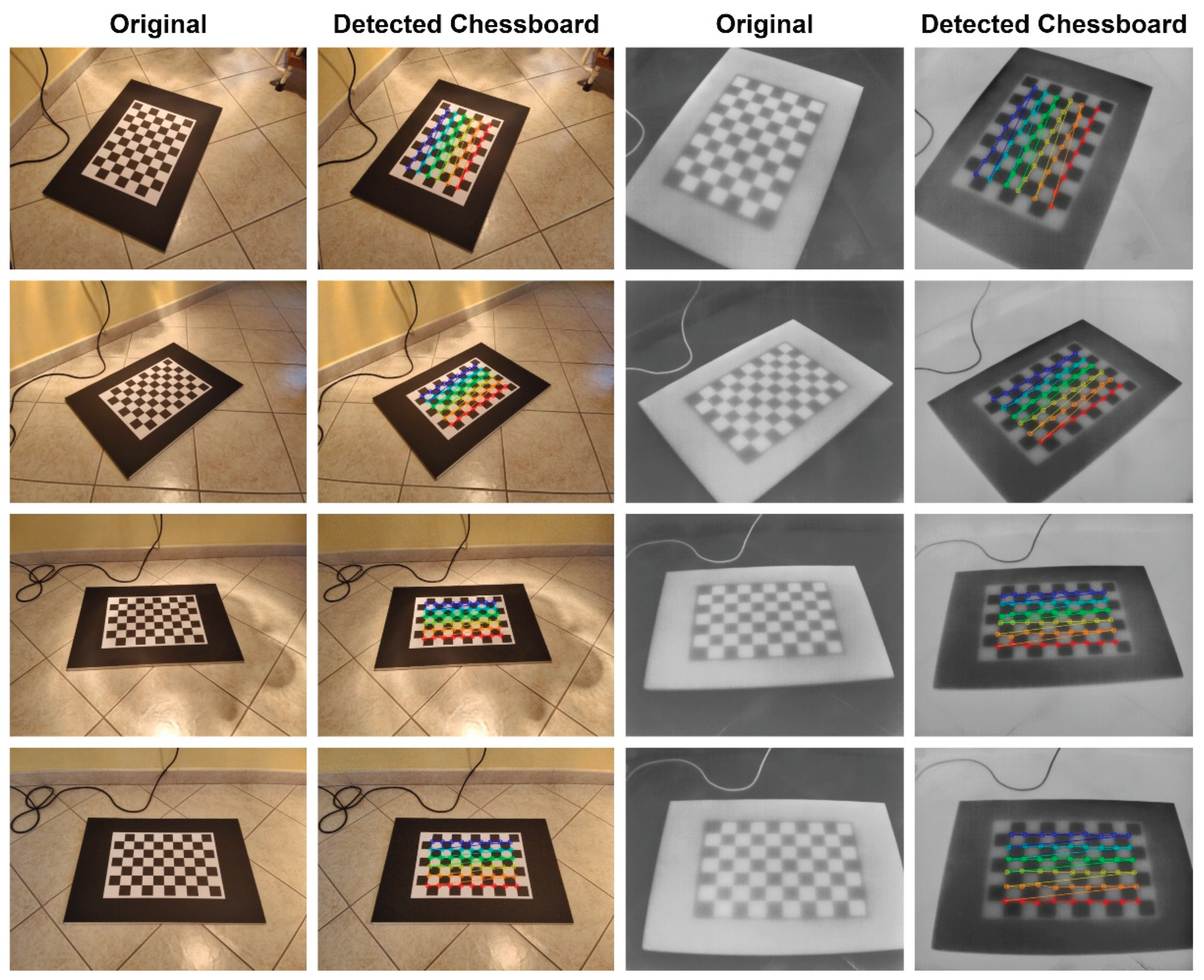
Figure 4.
Image undistortion process: (a) workflow; (b) implementation in Agisoft Metashape.
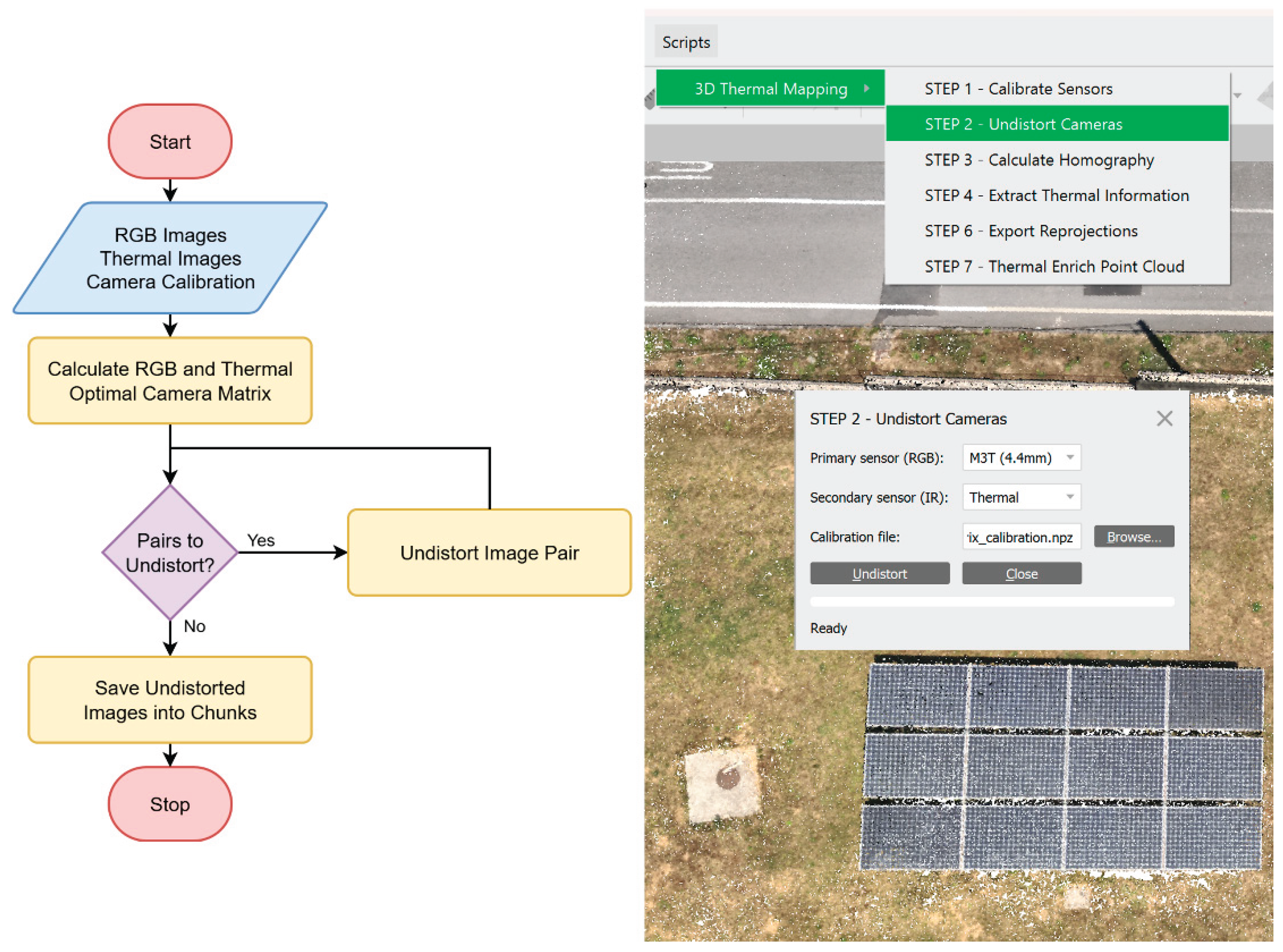
Figure 5.
Comparison of original and undistorted images on a subset of 4 pairs (RGB on the left and thermal on the right).
Figure 5.
Comparison of original and undistorted images on a subset of 4 pairs (RGB on the left and thermal on the right).
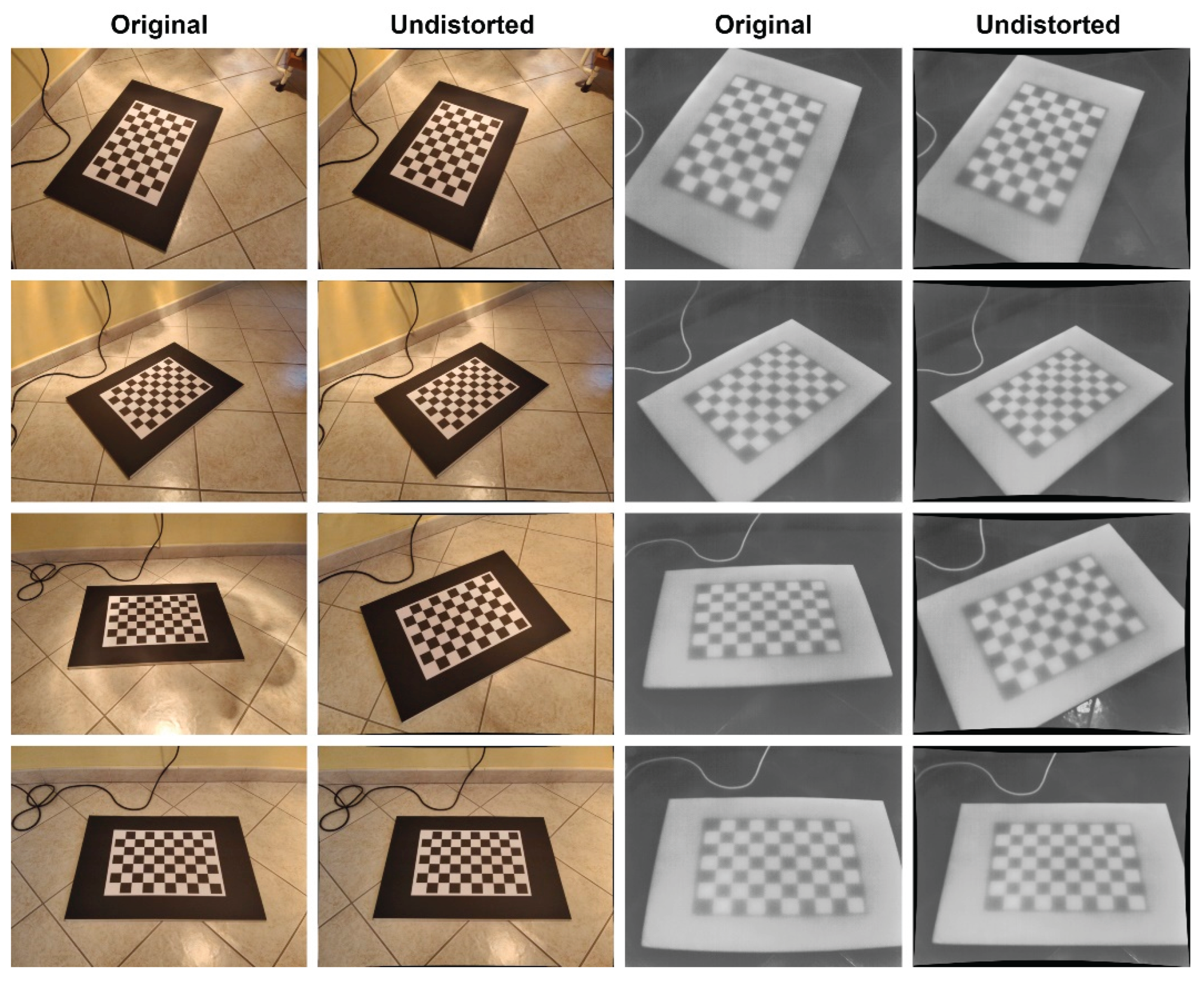
Figure 6.
Homography estimation process: (a) matching and transformation workflow; (b) implementation in Agisoft Metashape interface.
Figure 6.
Homography estimation process: (a) matching and transformation workflow; (b) implementation in Agisoft Metashape interface.
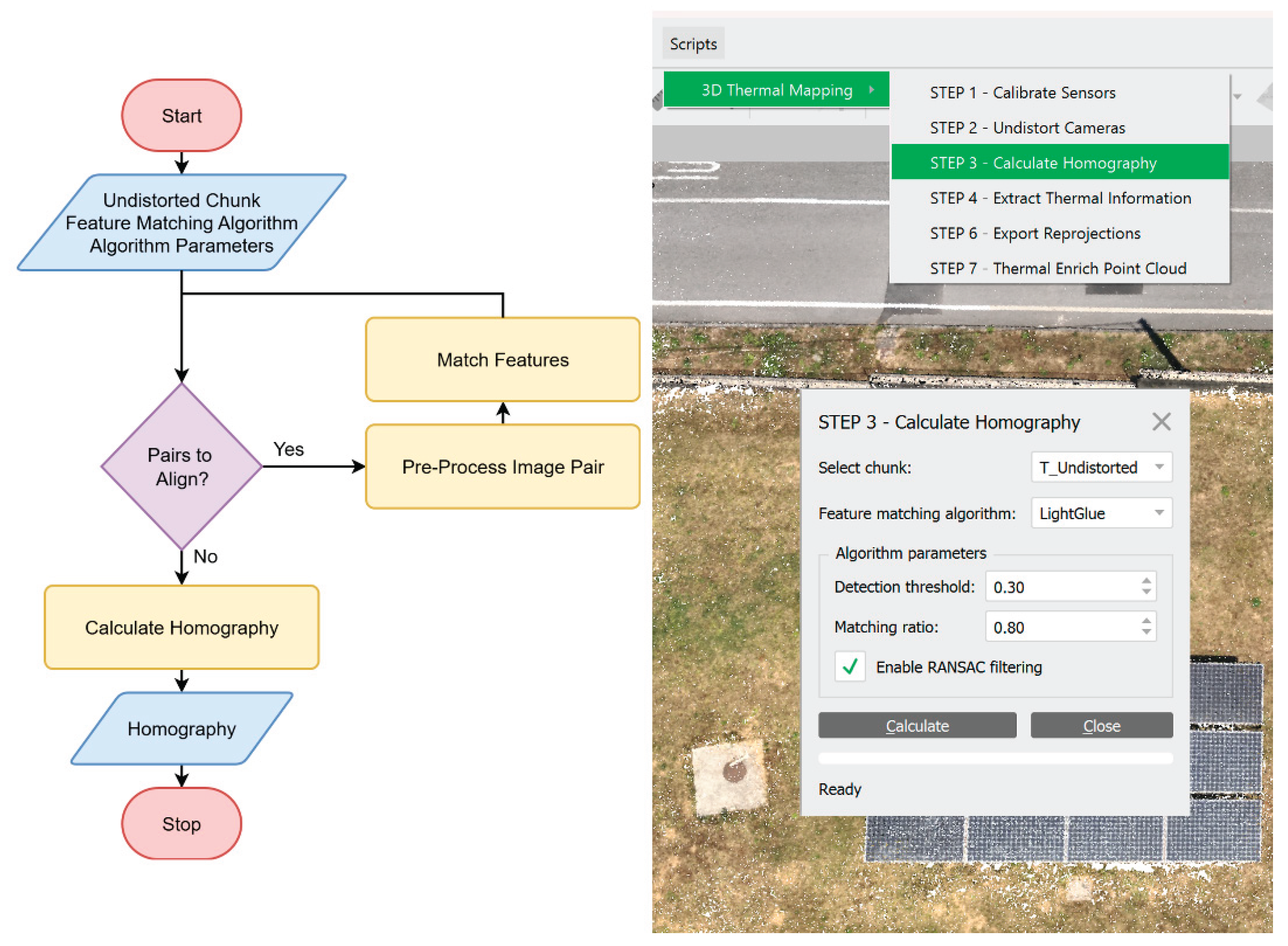
Figure 7.
Thermal data extraction: (a) workflow diagram; (b) implementation in Agisoft Metashape interface.
Figure 7.
Thermal data extraction: (a) workflow diagram; (b) implementation in Agisoft Metashape interface.
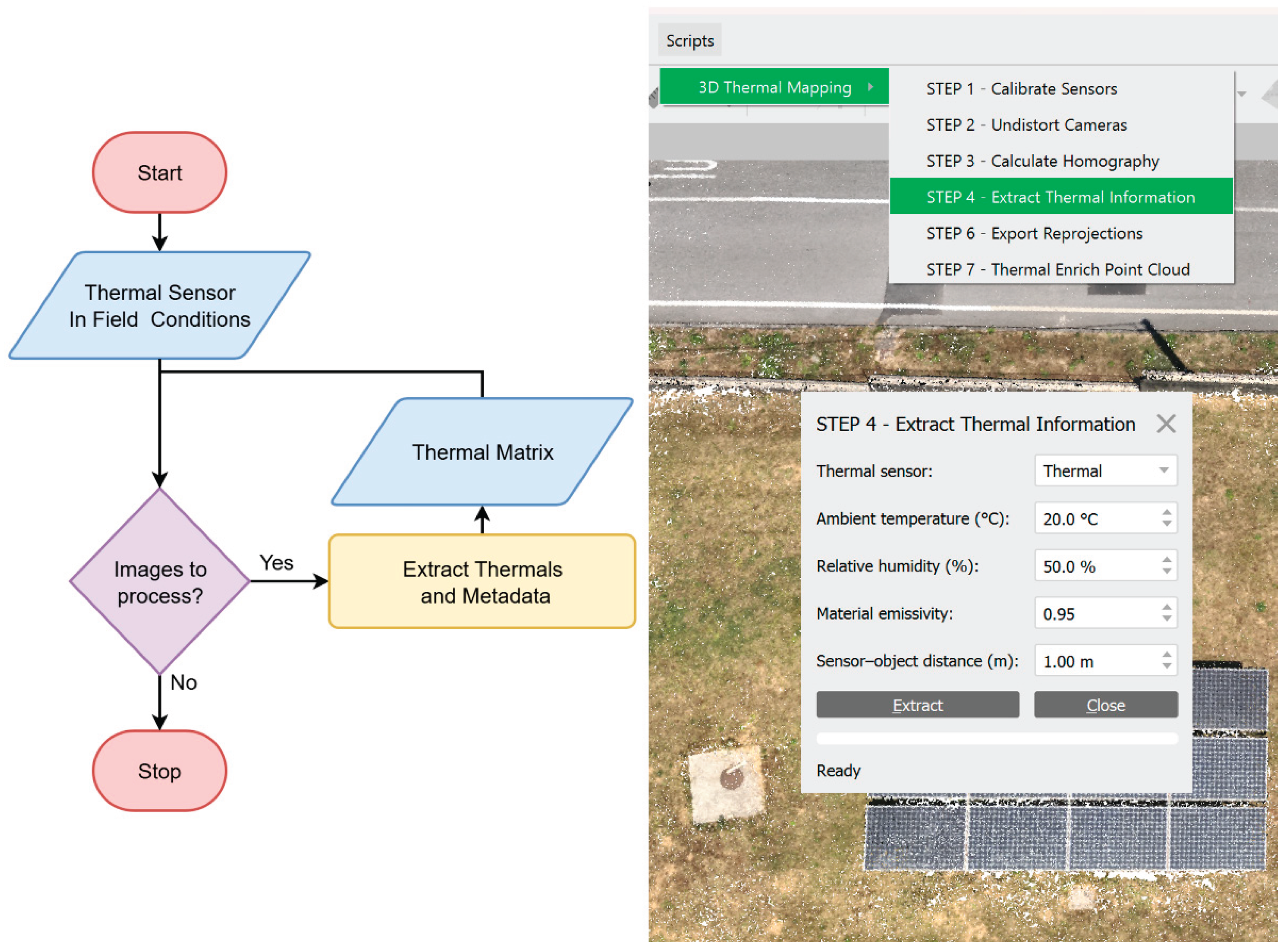
Figure 8.
Flight planning interface showing the automated survey grid over the area of interest.
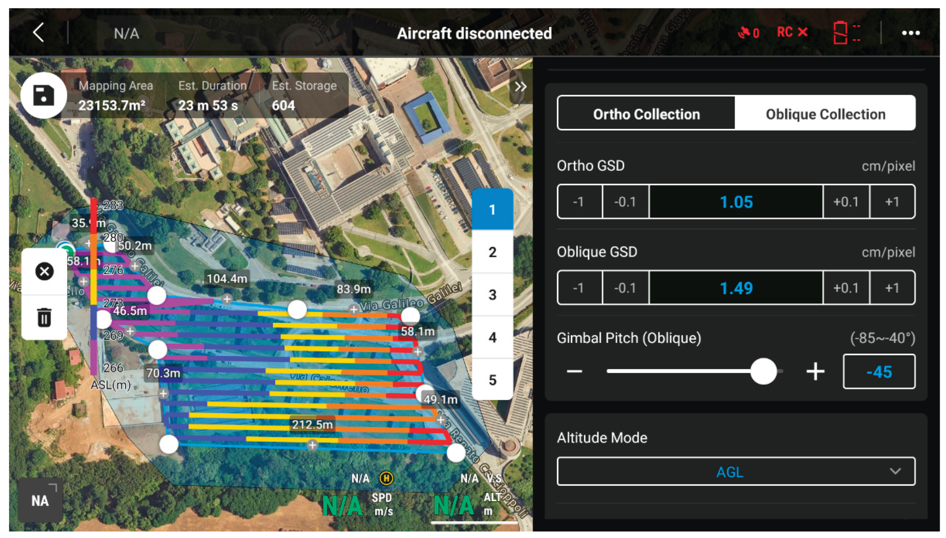
Figure 9.
Workflow diagram for the generation of the high-resolution RGB point cloud.
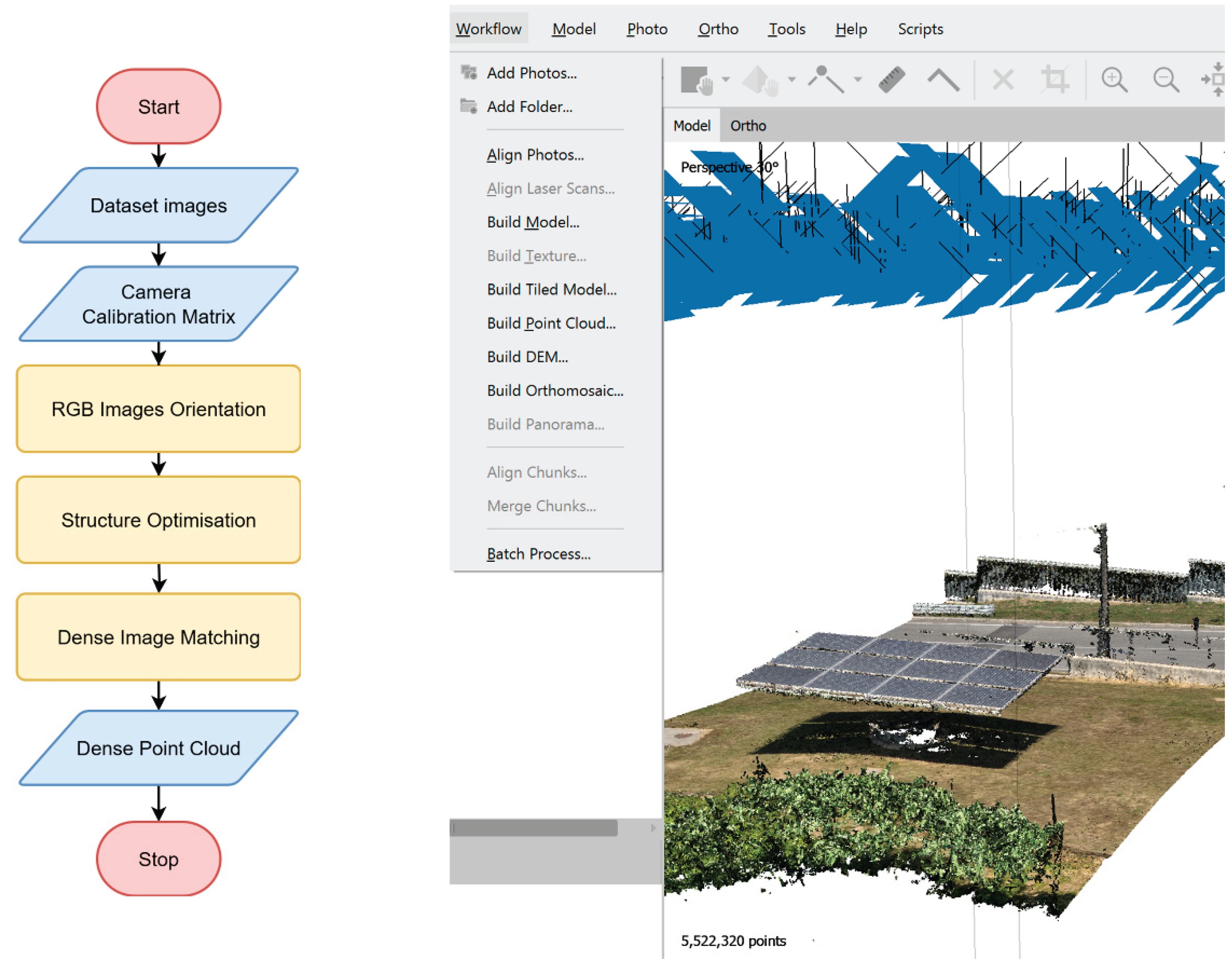
Figure 10.
Point cloud generated from the RGB dataset using Agisoft Metashape.
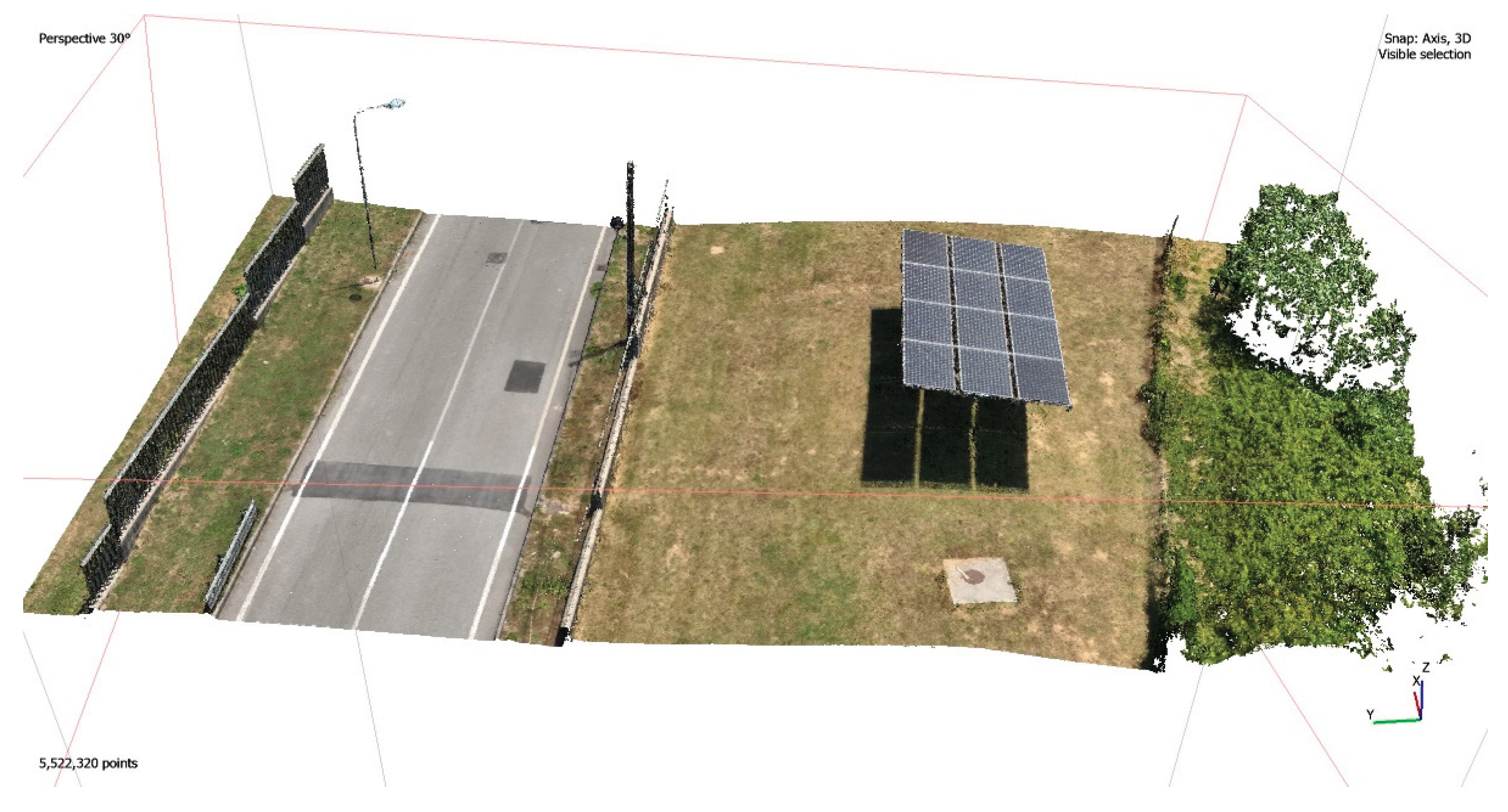
Figure 11.
Reprojection extraction: (a) workflow diagram; (b) implementation in Agisoft Metashape interface.
Figure 11.
Reprojection extraction: (a) workflow diagram; (b) implementation in Agisoft Metashape interface.
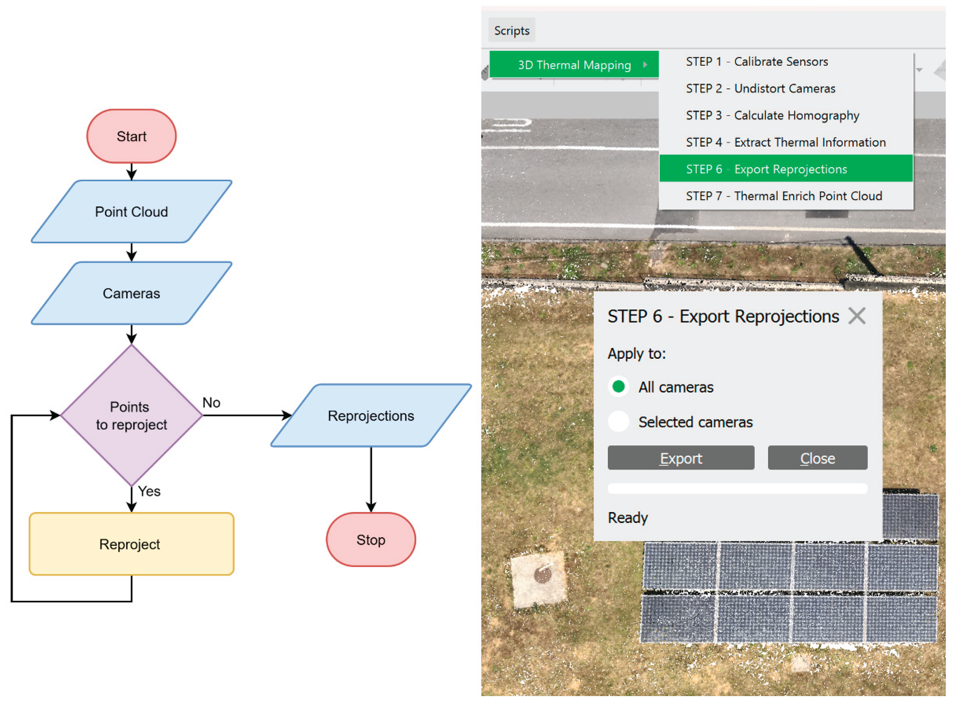
Figure 12.
Point cloud enrichment process: (a) workflow diagram; (b) result in Agisoft Metashape interface.
Figure 12.
Point cloud enrichment process: (a) workflow diagram; (b) result in Agisoft Metashape interface.
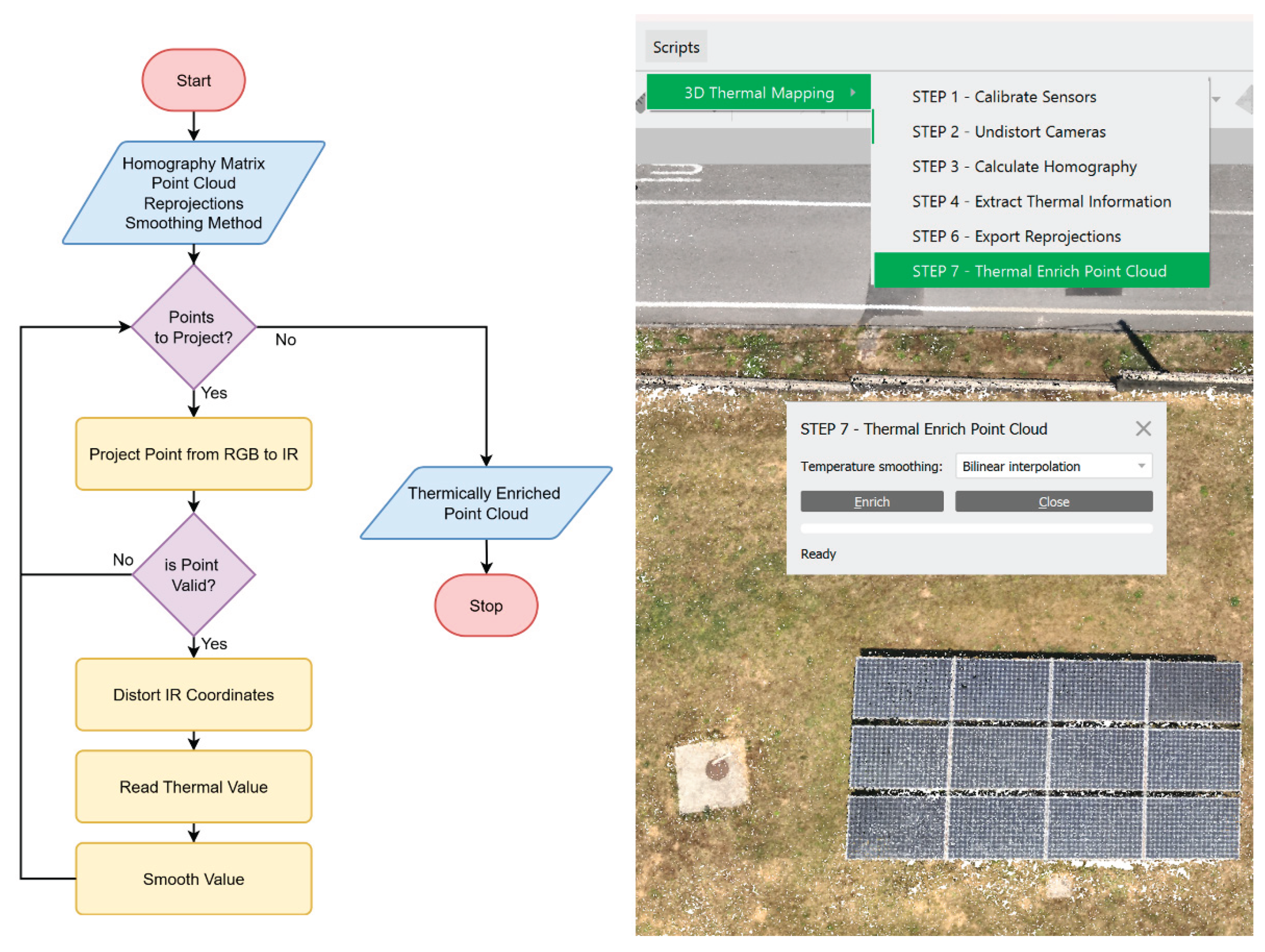
Figure 13.
Feature Matching between RGB and Thermal Images.
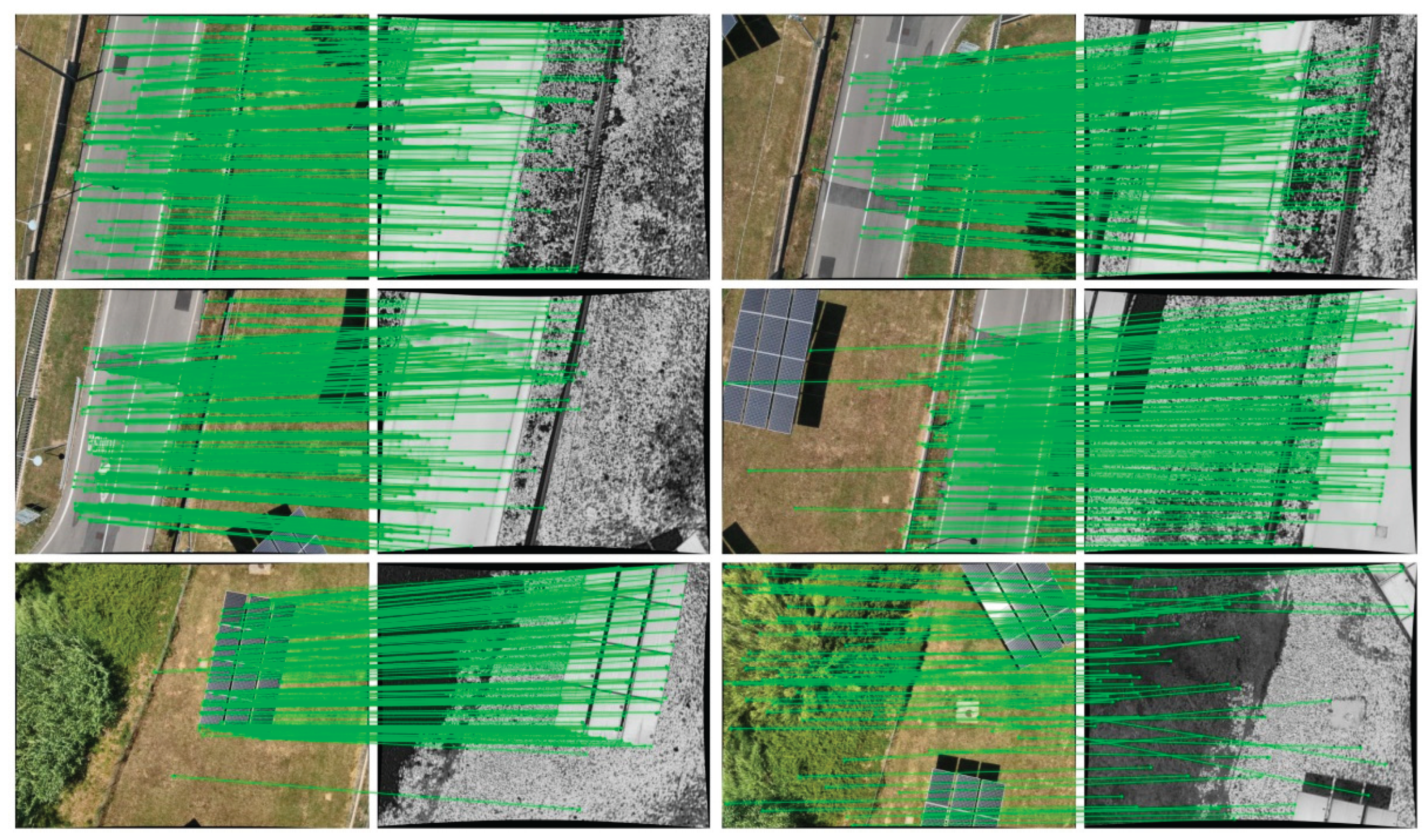
Figure 14.
Composite Overlay of RGB and thermal images.
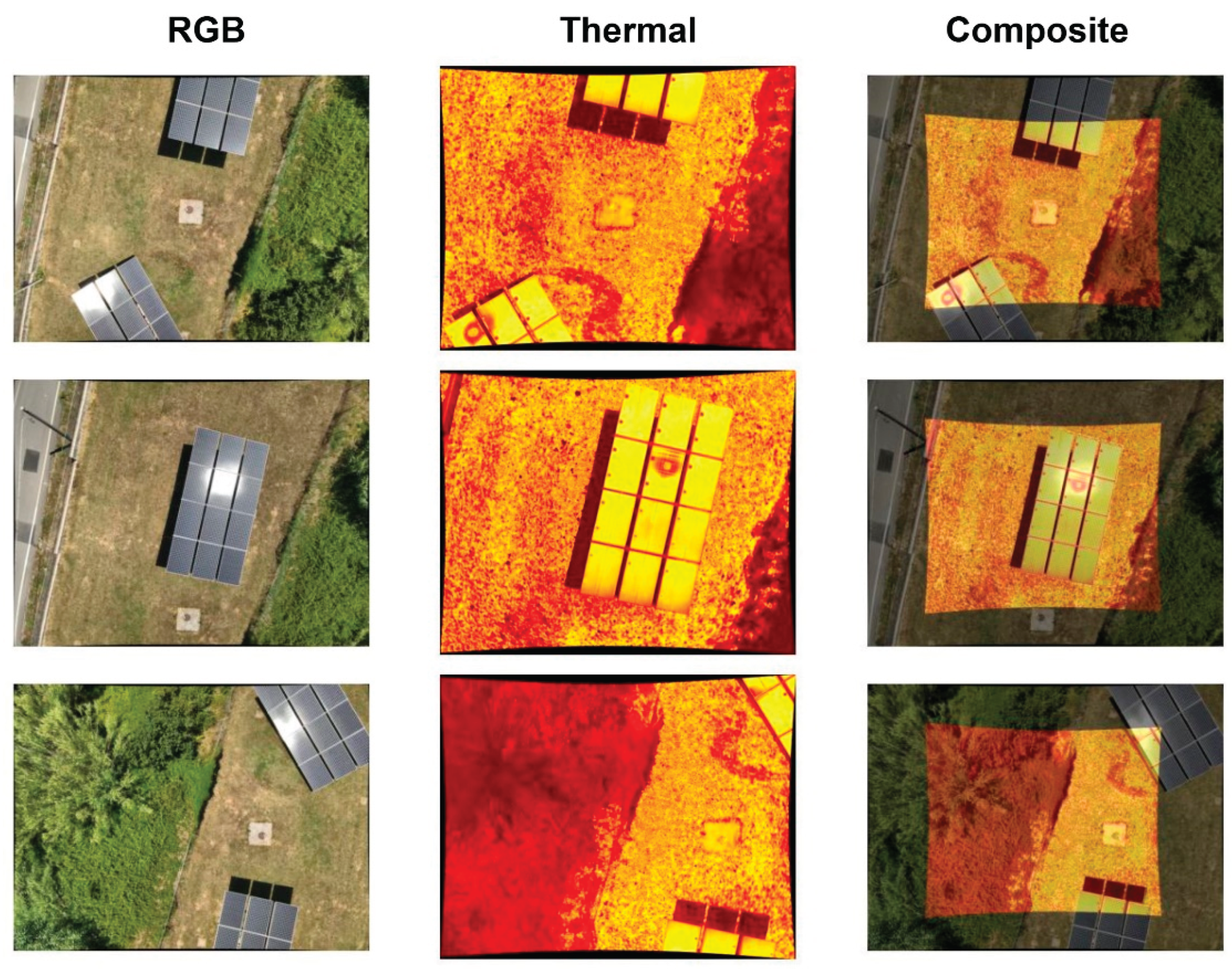
Figure 15.
Point Clouds: (a) Photogrammetric; (b) Thermally Enriched.
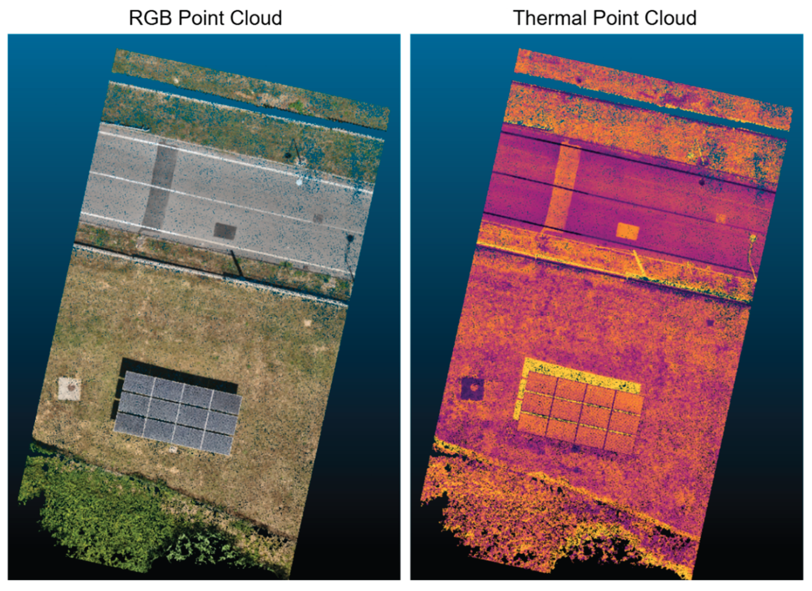
Figure 16.
Visual comparison of feature matching results across three algorithms: projection of correspondences between RGB and thermal images and composite images using the obtained homography.
Figure 16.
Visual comparison of feature matching results across three algorithms: projection of correspondences between RGB and thermal images and composite images using the obtained homography.
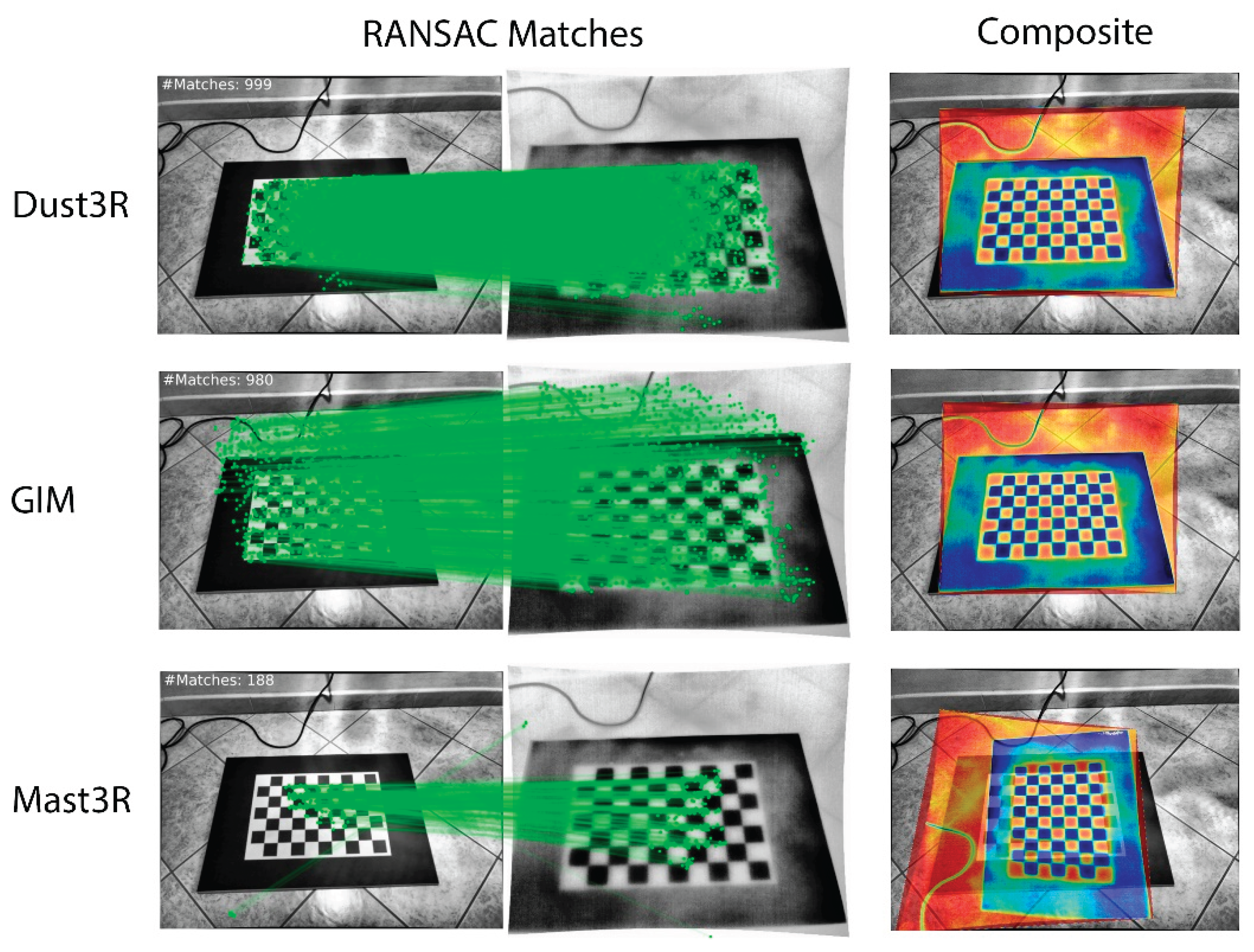
Figure 17.
Composite IR over RGB images in the calibration environment: overlay of thermal and RGB images using the computed homography.
Figure 17.
Composite IR over RGB images in the calibration environment: overlay of thermal and RGB images using the computed homography.
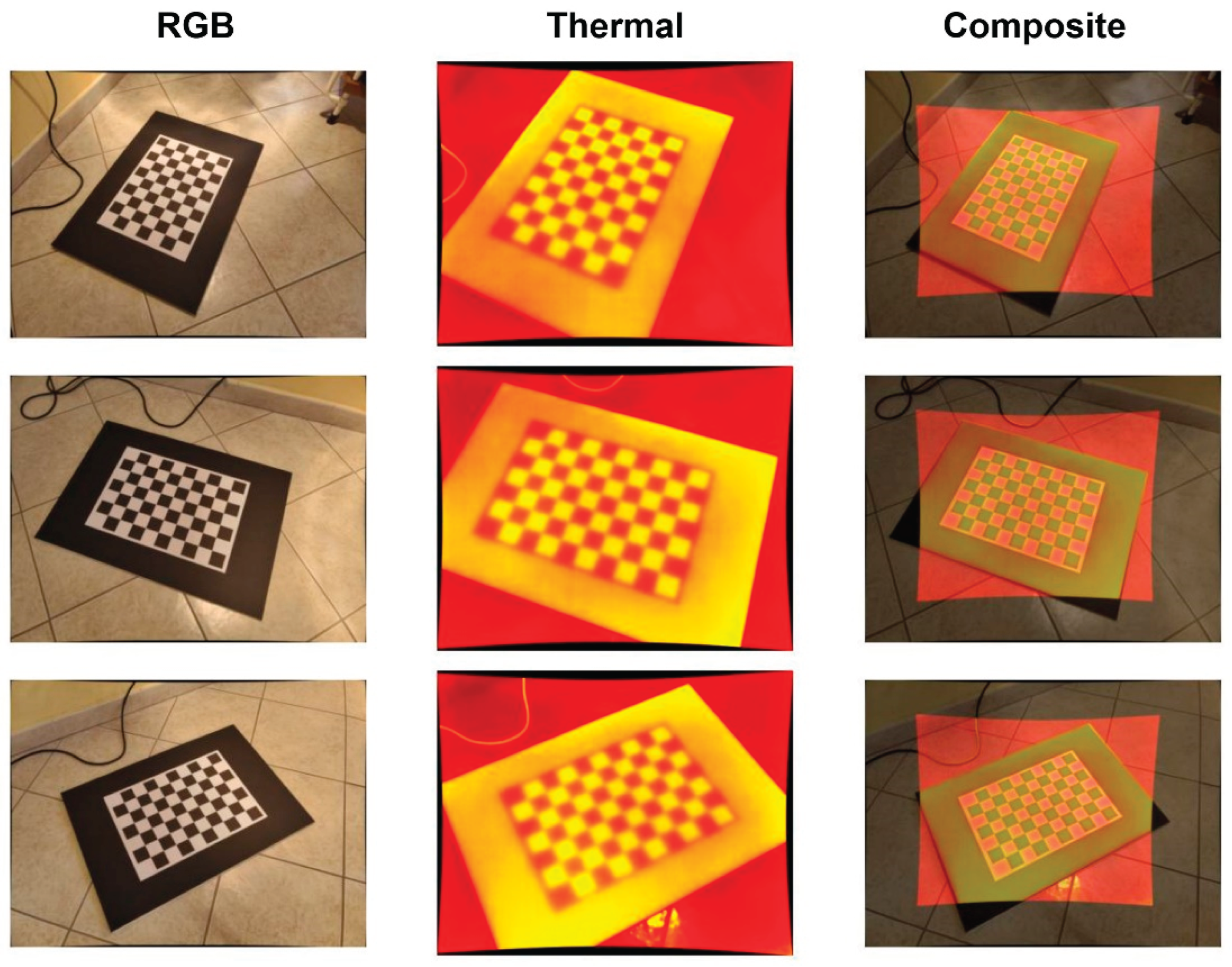
Figure 18.
Thermal matrix extracted from a region of interest: numerical values overlaid on a colour-coded temperature distribution.
Figure 18.
Thermal matrix extracted from a region of interest: numerical values overlaid on a colour-coded temperature distribution.
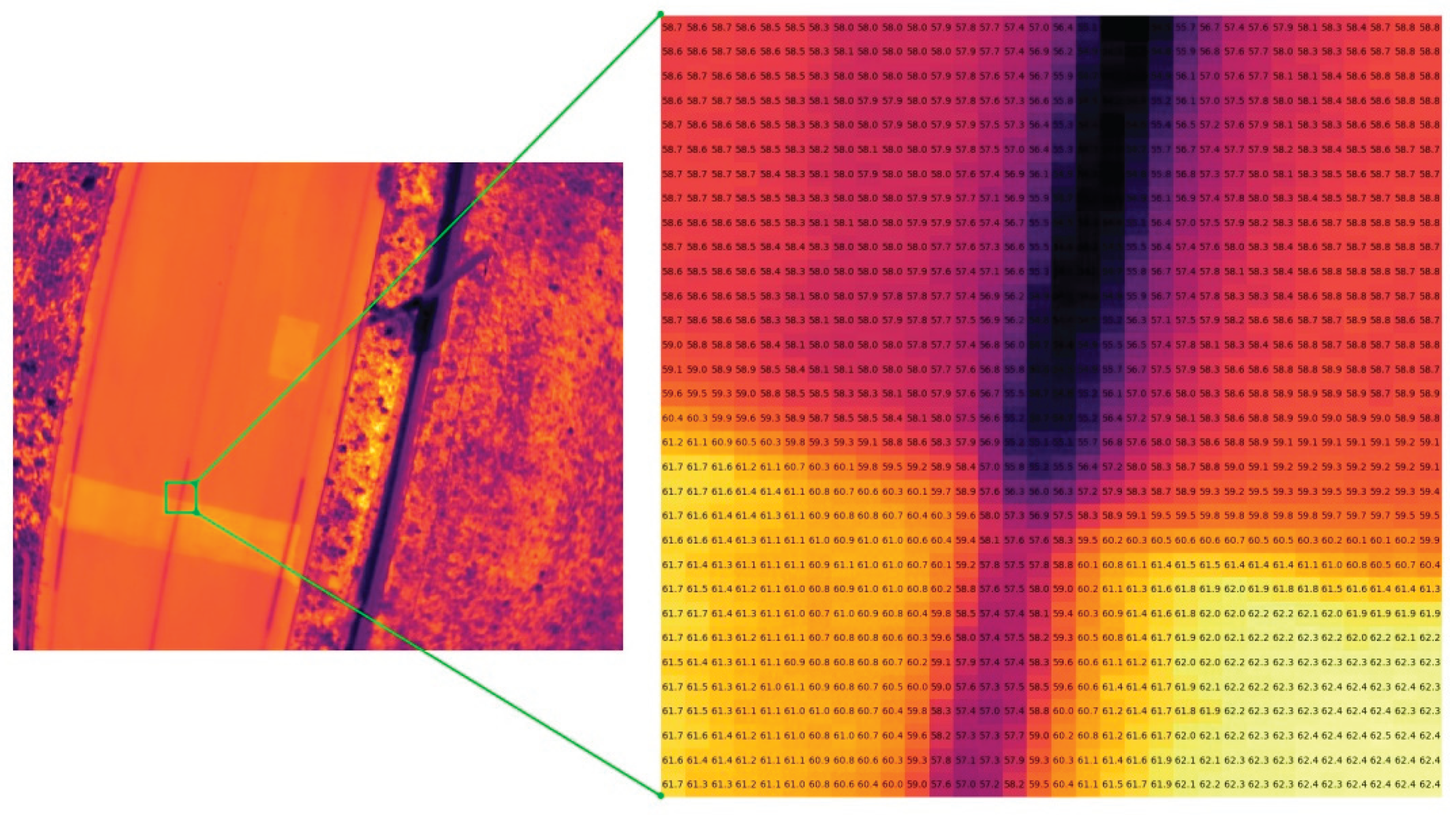
Figure 19.
View of the thermally enriched 3D point cloud, with temperature encoded by a colour gradient. A region of interest and its corresponding thermal image are also shown.
Figure 19.
View of the thermally enriched 3D point cloud, with temperature encoded by a colour gradient. A region of interest and its corresponding thermal image are also shown.
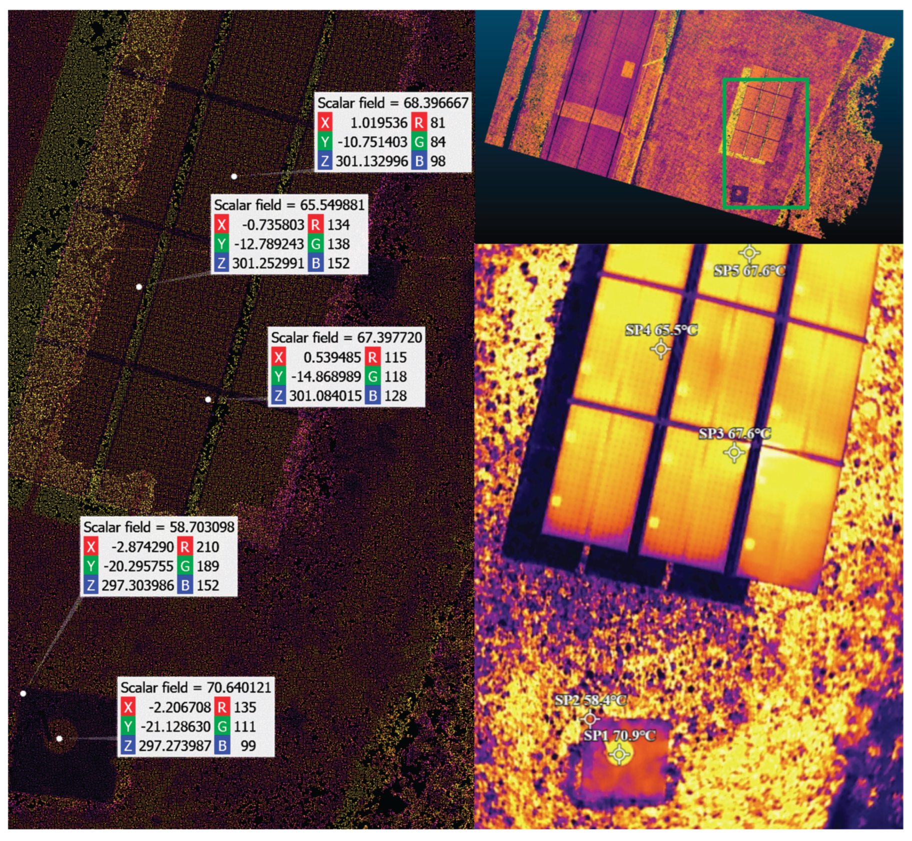

Table 1.
Technical specifications of the RGB and thermal systems onboard the DJI Mavic 3T.
| Wide Camera | Thermal Camera | Tele Camera | |
|---|---|---|---|
| System | 1/2-inch CMOS | Uncooled VOx Microbolometer | 1/2-inch CMOS |
| Resolution | 48MP - 8000x6000 (1) 12MP - 4000x3000 |
640x512 | 12MP - 4000x3000 |
| FOV | 84° | 61° | 15° |
| Aperture | f/2.8 | f/1.0 | f/4.4 |
| Focus | 1m to ∞ | 5 m to ∞ | 3 m to ∞ |
| Infrared Wavelength | N/A | 8-14 μm | N/A |
| Temperature Range | N/A | -20° to 150° C (2) 0° to 500° C (3) |
N/A |
| Infrared Accuracy | N/A | ±2° C or ±2% (4) | N/A |
| NETD | N/A | ≤50 mK@F1.0 | N/A |
(1) Shooting 48MP photo does not support 2s interval; (2) High Gain Mode; (3) Low Gain Mode; (4) using the larger value.
Table 2.
Software, tools and library versions used.
| Software | Version | Build | Channel |
|---|---|---|---|
| Agisoft Metashape Pro | 2.2.0 | 19135 | N/A |
| Python | 3.8.20 | h8205438_0 | N/A |
| OpenCV | 4.10.0 | py38hd762f8c_0 | conda-forge |
| Numpy | 1.24.3 | py38h1d91fd2_0 | conda-forge |
| PyTorch | 2.2.2 | py3.8_cuda11.8_cudnn8_0 | pytorch |
| PyTorch-CUDA | 11.8 | h24eeafa_6 | pytorch |
| MatplotLib | 3.7.2 | py38haa244fe_0 | conda-forge |
| CUDA | 11.8 | N/A | nvidia |
| DJI Thermal SDK | 1.7 | 20241205 | N/A |
| ExifTool | 13.21 | N/A | N/A |
Table 3.
Feature matching algorithm evaluated.
| matches | Error (px) | AUC (%) | ||||||
|---|---|---|---|---|---|---|---|---|
| Algorithm | # | % | μ | med | P95 | @1px | @3px | @5px |
| DeDoDe | 6 | 30 | 32.49 | 32.65 | 43.66 | 0.0 | 0.0 | 0.0 |
| Dust3R | 999 | 99.9 | 3.17 | 3.11 | 4.12 | 0.0 | 5.61 | 36.57 |
| EfficientLoF | 476 | 47.6 | 1.08 | 1.09 | 1.84 | 15.0 | 64.10 | 78.46 |
| GIM (RoMa) | 969 | 96.9 | 1.68 | 1.73 | 2.42 | 3.59 | 44.17 | 66.45 |
| GIM (dmk) | 980 | 98.0 | 1.40 | 1.50 | 1.99 | 6.96 | 53.36 | 72.02 |
| LiftFeat | 39 | 20.9 | 3.54 | 3.71 | 5.23 | 0.01 | 11.37 | 29.74 |
| LightGlue | 99 | 99.0 | 1.05 | 1.00 | 1.78 | 18.21 | 65.09 | 79.01 |
| Mast3R | 188 | 18.8 | 86.41 | 93.93 | 120.81 | 0.00 | 0.0 | 0.0 |
| OmnieGlue | 87 | 95.6 | 1.13 | 1.12 | 1.83 | 13.99 | 62.44 | 77.47 |
| RDD | 357 | 95.2 | 1.45 | 1.47 | 2.14 | 5.22 | 51.81 | 71.05 |
| SuperGlue | 98 | 98.0 | 1.05 | 1.04 | 1.80 | 17.53 | 64.99 | 79.03 |
| XoFTR | 384 | 38.4 | 1.13 | 1.16 | 1.86 | 14.72 | 62.38 | 77.41 |
Disclaimer/Publisher’s Note: The statements, opinions and data contained in all publications are solely those of the individual author(s) and contributor(s) and not of MDPI and/or the editor(s). MDPI and/or the editor(s) disclaim responsibility for any injury to people or property resulting from any ideas, methods, instructions or products referred to in the content. |
© 2025 by the authors. Licensee MDPI, Basel, Switzerland. This article is an open access article distributed under the terms and conditions of the Creative Commons Attribution (CC BY) license (http://creativecommons.org/licenses/by/4.0/).
Copyright: This open access article is published under a Creative Commons CC BY 4.0 license, which permit the free download, distribution, and reuse, provided that the author and preprint are cited in any reuse.


