
Submitted:
04 December 2024
Posted:
06 December 2024
You are already at the latest version
Abstract
Point clouds are a crucial element in the process of scanning and reconstructing 3D environments, such as buildings or heritage sites. They allow for the creation of 3D models that can be used in a wide range of applications. In some cases, however, only the 3D model of an environment is available, and it is necessary to obtain point clouds with the same characteristics as those captured by a laser scanner. For instance, point clouds may be required for surveys, performance optimization, site scan planning or validation of point cloud processing algorithms. This paper presents a new Terrestrial Laser Scanner (TLS) simulator, designed as an Blender add-on, that produces synthetic point clouds from 3D models in real-time, while adhering to standard laser scanner parameters. The target meshes may be derived from either a real-world scan or 3D designs created using design software. The simulator generates point clouds with distributions and characteristics similar to those obtained by a real laser scanner, incorporating the standard parameters from scanner specification sheets. This feature, together with its real-time generation capability, makes it particularly suitable for scan planning and the creation of synthetic point cloud repositories.
Keywords:
Virtual laser scanner
; point clouds
; scan plannong
; dataset generation
; geometry nodes
; Blender
1. Introduction
Laser scanners have undergone significant developments over the past two decades, and it seems likely that this trend will continue in the near future. Since their inception, three-dimensional (3D) scanning technologies have ushered in a new era of applications in an expanding range of disciplines, including architecture, engineering, construction, healthcare, entertainment, manufacturing and cultural heritage preservation, among others [1]. Currently, an increasing number of projects in all fields require accurate, high-quality three-dimensional point clouds, which can only be obtained with laser scanners.
Despite the availability of sophisticated commercial 3D scanners, the high cost and specialized hardware requirements often restrict their accessibility, particularly for small businesses, educational institutions, and independent developers. Besides, the acquisition of point clouds is a lengthy, costly, complex, and occasionally dangerous or impossible process [2,3]. These factors have led to a shortage of large point cloud data sets. One potential solution to this issue is the generation of synthetic data.
The generation of synthetic point clouds has been a topic of particular interest within the computer vision community. This process is complex and requires careful research and strategizing to establish an effective procedure that ensures the properties of the synthetic data aligns closely with those of the real data, which will permit the synthetic data to be used as substitutes for the real data.
Consequently, numerous researchers have explored the use of synthetic datasets in a variety of fields to address specific needs and applications.
In general, the different methods proposed in the literature can be classified into two primary categories: those that create synthetic point clouds by sampling existing geometric models and those that generate them from a scanner simulator.
Among the approaches that utilize existing models, [4] presents a procedure his method involves the use of three different software tools to convert 3D models into synthesized point clouds.: Autodesk Revit [5] for developing the 3D models, Trimble SketchUp [6] for importing them, and Safe Software FME desktop workbench [7] to transform SketchUp files into synthetic point clouds. In [8], a bottom-to-top methodology is proposed for the automated generation of synthetic bridge geometries. This approach assembles complete bridge models from primitive shapes. The resulting synthetic dataset is designed to approximate the geometric properties of two types of real masonry arch bridges: straight and curved bridges. To replicate geometric distortions and laser scanning errors that typically occur in practice, a noise-free synthetic point cloud is initially generated from sampling these models. Subsequently, random noise is introduced to simulate realistic conditions. Also, in the field of bridges, [9] explores two distinct methodologies for generating synthetic point clouds. Both approaches start with the creation of 3D geometric models of the truss bridges. From these models, uniform point clouds are produced by uniformly sampling of the mesh surface points. To produce point clouds with occlusion, a TLS (terrestrial laser scanning) simulator is employed. The procedure entails specifying the positions of the virtual TLS in the target environment and defining the angular pitch to emulate a scanning operation. For its implementation, the Open3D [10] ray casting function is used to project rays from each virtual scanner position and compute the impact points where the rays intersect with the surrounding mesh surfaces. More examples of synthetic data generation by surfaces sampling are reported in [11], where Grasshopper visual programming has been leveraged to define parametric shapes of historical dome systems, which are then converted to mesh and subsampled in CloudCompare; [12], in which Zhai et al. present subsampling IFC and complementary OBJ models for generating labeled point clouds with coordinates and color data; and [13], that presents an approach for automatic generation of synthetic dataset of point clouds for Cultural Heritage field.
The second major category is that of scanning simulations, which represents a more sophisticated technique. It entails the generation of synthetic scanners that emulate the operational characteristics of their real-world counterparts. BlenSor [14] is one of the most well-known proposals in the field. It is a unified simulation and modeling environment capable of simulating several different types of sensors, considering their physical properties. It is based on ray tracing and incorporated as a standalone tool within the Blender software suite [15]. BlenSor provides the capability to develop algorithms for the sensors it simulates without the necessity of physically owning a sensor. Additionally, it allows for the simulation of situations that would otherwise be unfeasible, as well as for the effective pre-planning of both scanner positions and scanning parameters (e.g., mounting height, angle, speed) prior to undertaking real-world scanning. BlenSor has been used in the work by Griffiths et al. [16] to generate SynthCity, an open, large-scale synthetic point cloud designed to facilitate research into the potential benefits of pre-training segmentation and classification models on synthetic data sets. Other researchers in the autonomous driving field have also contributed to enhancing real datasets with synthetic data obtained from LiDAR simulators [17,18,19]. In [20], BlenSor is used for generating synthetic point clouds from IFC models, and for FBX models in [21]. Korus et al. developed DynamoPCSim [22], another Terrestrial Laser Scanning (TLS) simulator also based on ray tracing. They have developed the simulator as a package to Dynamo [23], an open-source visual programming environment, that provides the base for geometrical processing. The simulator can utilize BIM models directly due to the linkage of Dynamo with Revit. The simulator's modular design, combined with the flexibility of visual programming, makes it adjustable to specific tasks, varying scanning attributes, desired point cloud parameters, and customizable automatically gathered labels. One more proposal of this nature is HELIOS++ [24], an open-source simulation framework for terrestrial static, mobile, UAV-based and airborne laser scanning implemented in C++. It has been employed with OBJ models that have been converted with Blender from IFC models that were originally created in Revit [25] or scenes that were generated directly in Blender [26]. Table 1 in [22] presents a comparative analysis of the three laser scanner simulators. Another interesting approach is the driving simulator CARLA [27] for a mobile scanning simulator [28], or the generation of the Paris-CARLA-3D dataset [29], which comprises a collection of dense, colored point clouds of outdoor environments. In the field of robotics, MORSE [30] is an open-source simulator for academic robotics that was discontinued in 2020. It is a generic robot simulator project that includes a LIDAR simulator that is not of the TLS type, but rather employs multilayer range sensors. The primary focus of this approach is the detection of objects in industrial settings. Similarly to MORSE, Gazebo [31] employs a configurable LIDAR, allowing the user to specify parameters such as maximum and minimum angles, resolution, and the potential for introducing noise to the obtained data. The VRScan3D simulator [32] is a comprehensive virtual reality (VR) tool for training and education in laser scanning techniques. The software enables users to simulate the entire procedure of data acquisition from a laser scanner, providing a realistic experience that allows them to virtually position the scanner within the scanning area, adjust its parameters, and undertake other essential steps involved in the scanning process.
Notwithstanding the existence of these efforts to develop simulation tools, there remains a lack of available solutions that provide sufficient control over the simulation parameters and properties of the acquired point clouds, emulate the performance of scanners, and do not require dedicated processes. To illustrate, Blensor is unable to function in real time. Gazebo does not appear to be readily configurable to align with the format typically seen in laser scanner data sheets (Xmm@Ym) and it lacks obstacle detection functionality. VRScan3D is primarily oriented towards an educational perspective.
Our approach addresses these limitations by introducing a TLS simulator that generates synthetic point clouds from 3D models in real time, adhering to the standard parameters of a laser scanner. The input meshes can be derived either from real-world scans converted into 3D meshes or from designs created using computer-aided design (CAD) software. By utilizing standard parameters from laser scanner specification sheets, the simulator produces point clouds with distributions and characteristics comparable to those of real-world laser-scanned data. This capability makes the tool highly versatile for a range of applications reliant on point cloud data. Specifically, it provides an efficient solution for scan planning and significantly aids in the creation of point cloud repositories, which are essential for testing and validating 3D processing algorithms.
The rest of the paper is structured as follows. Section 2 begins with the brief description of the geometry nodes tool interface in Blender, followed by an explanation of the methodology used to develop our Real time TLS. Section 3 presents the experimental validation of the proposal. Finally, Section 4 presents a discussion on the results obtained.
2. Materials and Methods
The real-time TLS simulator that we propose is an add-on of the open-source software Blender [15]. The add-on development is based in Blender Python API and in Visual Programming Tools (VPL) included in Blender. These tools permit the creation of algorithms that procedurally generate a great variety of Blender geometries and operations. In this case, the VPL tool employed is Geometry Nodes, a node-based system designed for modifying the geometry of an object or generating new associated geometries. This system operates by taking an input geometry and producing an output geometry through the creation of a network of interconnected nodes. Within this network, nodes can be grouped into higher-level nodes to streamline the representation of the network, resulting in a tree structure of nodes that can encompass various levels of depth and complexity.
Figure 1 depicts the default Geometry Nodes’ Blender interface in programming mode. The 3D environment is displayed in the upper right quadrant, with the objects present therein. The upper left quadrant presents pertinent information about the object being created by geometry nodes in real time, including the number and position of its vertices, edges, or faces. The lower quadrant illustrates the visual programming area of the geometry nodes.
As illustrated in Figure 1, the geometry nodes, situated in the lower panel, facilitate the creation and editing of any type of geometry in real time by allowing the addition and interconnection of nodes with varying functionalities. Any changes made to the nodes are automatically reflected in the 3D environment, enabling the manipulation of complex geometric structures in a dynamic and efficient manner.
The illustration depicts the generation of a sphere through the transfer of the output parameter ‘Mesh’ from the UV sphere node to the Group Output node, which is responsible for displaying the generated geometry on the screen.
The add-on is based on the creation of 'scanner' objects in the scene, to which a 'Geometry nodes' modifier is assigned, which implements the scanning process of the selected scene meshes. Figure 2 shows the geometry node tree generated by the add-on.
The basic operation, summarized in the diagram in Figure 3, starts with a mesh or set of meshes of the scene to be scanned and a set of user input parameters. Internally, a virtual scan of these meshes is performed, resulting in a set of scanned points on the mesh surfaces. A filter is then applied to these points to eliminate those that cannot be scanned because they are under the device where the laser is not emitted, thus simulating the limitations imposed by the constructive dispositions of the laser scanners. Next, it is possible to modify the colors associated with the results of the scans. Finally, the possibility of configuring various parameters of the 3D representation of the result is offered. Furthermore, to complete the process, the add-on allows the generation of files that store the scan data or that show a scanning map.
The following sections describe each block of this schema in more detail.
2.1. Scanning Simulation
The node on which the virtual scanning function is based is the Scanner node. This node contains a tree (Figure 4) that consists of three main blocks: Sphere Scanner, Scanner Model, Point Deletion and Transform Points.
Specifically, the origin of the scan is inside the Sphere Scanner block, where a UV sphere is created whose vertices are the points that will be projected onto the environment. This sphere is composed of quadrilaterals (formed by two coplanar triangles), as the one shown in Figure 5a, and is characterized by its radius and the number of rings and segments that define it (Figure 5b, c). The scanner simulation procedure is based on launching rays that pass through the vertices of the sphere and whose orientation coincides with the normal vectors of these vertices, as shown in Figure 5d - f. The parameters that define the laser emission simulation process are the emission angle and the range of the lasers, shown in Figure 5g. Of these two, the one that affects the creation of the UV sphere primitive is the angle. Thus, the smaller the angle, the more rings and segments will form the sphere. Therefore, if ϕ is the angle entered by the user in degrees, obtaining the number of rings, r, and segments, s, fulfills the relationships of the following equations:
This last condition is necessary to make the sphere regular in terms of face sizes. Regarding the radius, it is sufficient to enter a small value in relation to the dimensions of the meshes to be acquired. A value of 1e-6 is considered acceptable for any mesh to be used.
2.1.1. Point Projection
Once the sphere has been generated with the required number of vertices, these vertices are projected onto the three-dimensional environment, thereby simulating the point cloud that would be obtained with an ideal laser scanner, which would not exhibit any type of error or deviation.
As with real laser scanners, the laser intersects with the surrounding surfaces and bounces off to be received back into the device. This process takes place within the Raycasting node shown in Figure 2, the contents of which are shown in Figure 6. The Raycast node is used to simulate this intersection process. The input parameters are ‘Target Geometry’ and ‘Ray Direction’. The former denotes the geometry of the 3D environment on which the ray’s intersection will be detected, while the latter indicates the direction, defined by a vector starting from the vertices of the sphere, in which each of them will be projected onto the environment. As the direction of projection coincides with the position vector of each vertex with respect to the sphere center, this position node is added as an input parameter.
The output parameters of this node are as follows. ‘Is Hit’ is a list of Booleans that indicate for each vertex whether it has intersected the geometry of the environment. ‘Hit Position’ is a list of vectors indicating, for each projected vertex of the sphere, the position where it intersected the 3D environment (Figure 9b). ‘Hit Distance’ is a list of floats indicating for each vertex of the sphere the distance from its center.
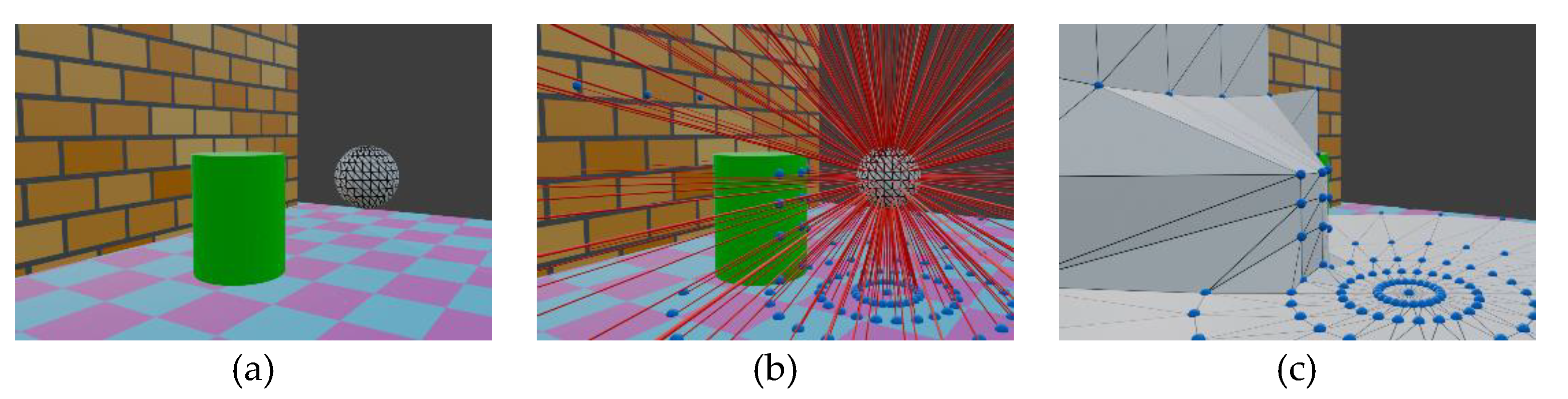
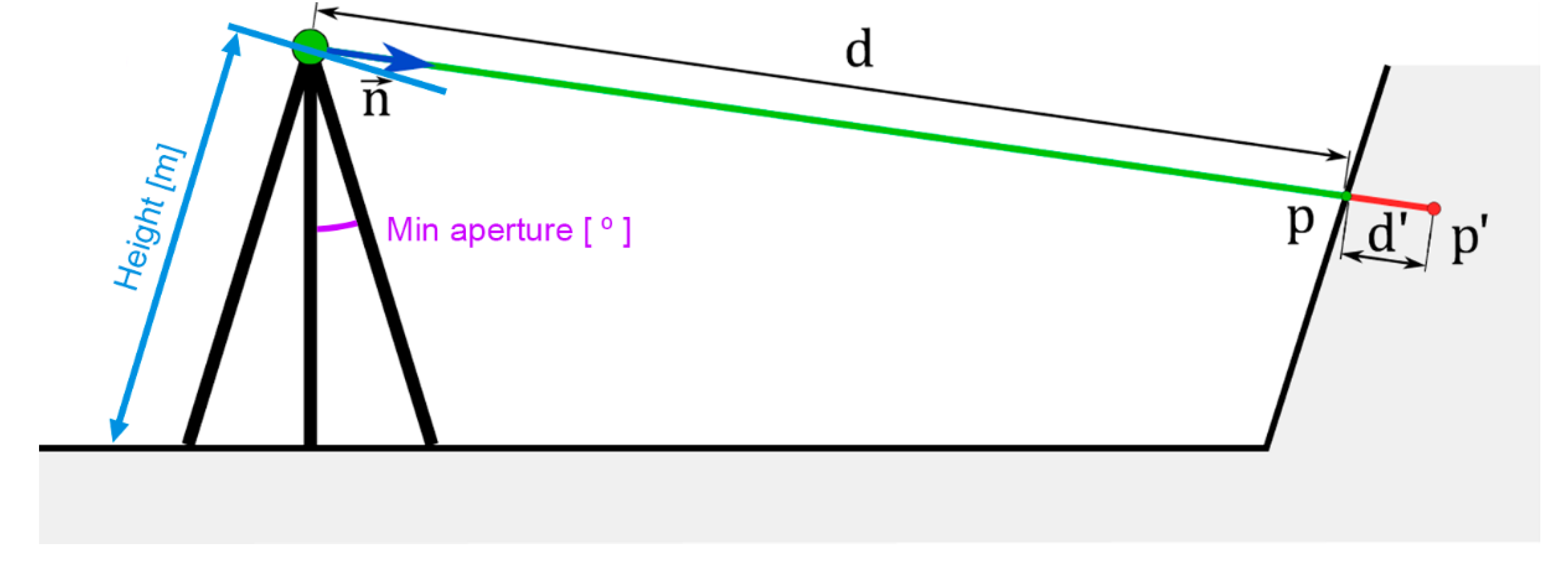
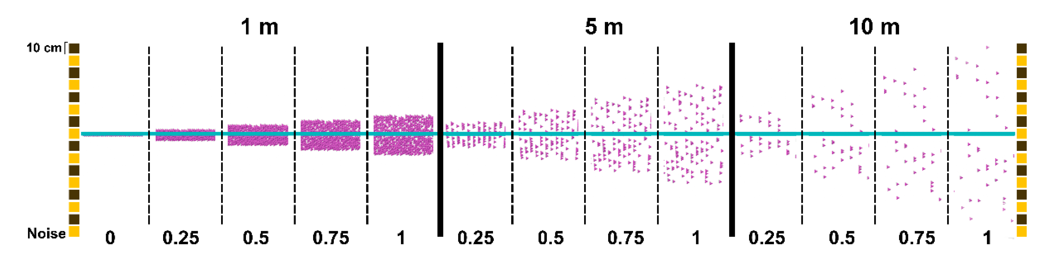
Figure 7.
(a) Example of simple set of meshes to be scanned (wall, floor and cylinder) by the scanner (wireframed UV sphere); (b) representation of the raycasting process and the intersection computed on every mesh (represented by blue spheres); (c) resulting mesh produces after translating the UV sphere points, keeping the definition of the original sphere faces.
Figure 8.
Calculation of point p from the distance d and the error d' and parameters of the scanner model: Height(m) and Min aperture ().
Figure 8.
Calculation of point p from the distance d and the error d' and parameters of the scanner model: Height(m) and Min aperture ().
Figure 9.
Noise.
Specifically, as shown in Figure 6, two Raycast nodes are used. The one above simulates the mesh scanning, and the one below is only used to compute the height of the scanner with respect to the mesh. That is why only one ray, (0, 0, -1), is used as direction input of the node.
Then, in the Transform Points block, the vertices of the scanner sphere are displaced to their final positions by means of the Set Position node. This node accepts as input parameters the geometry to be modified (the sphere), the list of final positions (intersection points obtained in the Raycast node), and a selection (list of points whose emitted rays intersect with mesh).
The output of this node is the geometry with the modified vertex positions, in this case with each vertex projected onto the geometry of the environment. Thus, the initial sphere scanner (Figure 7a) is transformed into a mesh whose vertices are over the acquired scanned meshes (Figure 7c), since the vertices have been translated but the faces are composed by the same edges.
The Set Position node also accepts another input parameter, designated as ‘Offset’. This parameter allows the user to enter a list of vectors, whose values are added element-wise to the positions indicated in the ‘Position’ input parameter. This enables the modification of the previously obtained positions by introducing a series of values, d', which depend on the distance d travelled by a point from its initial position to the position where it intersects with the 3D geometry of the environment to be scanned, and on a user-defined tolerance parameter tol for the laser scanner.
The tolerance parameter tol is further modified by applying white noise (w) to introduce randomness in the displacement of the points in opposite directions. To achieve this, the White Noise Texture node generates random values in the range following a white noise pattern. These values are then mapped to the range using the Subtract node.
Once the values of the previously mapped white noise, , are multiplied by the parameter , the resulting displacements are adjusted based on the assumption of a linear relationship between the point dispersion produced by the laser scanner and the distance to the scanner. Thus, the error at a distance of m will be approximately ten times smaller than the error at a distance of m.
Consequently, the noise value is sequentially multiplied by the tolerance parameter tol and the distance of the point to the scanner, resulting in the offset .
The coordinates of the projected points, prior to the addition of noise and denoted by , can be expressed as:
Here, represents the vectors that define the line connecting the scanner and the projected points, which are the normal vectors of the sphere vertices emitting the rays that project the points.
Therefore, after applying the noise, the coordinates of the points are given by:
This transformation is implemented in the Set position node, where the inputs are the coordinates and the offset .
A conceptual representation of the noise-induced offset is shown in Figure 8. On the other hand, Figure 9 depicts the top view of several pink point clouds produced after scanning a wall located at distances of 1, 5 and 10 meters from the scanner and using different values of the tol parameter: 0, 0.25, 0.5, 0.75 and 1.
2.2. Model Scanner and Point Delection
To assist the user in positioning the scanner, a schematic model of the scanner on a tripod can be displayed. The parameters that can be modified are the length of the tripod legs and the minimum opening angle of the tripod legs, as shown in Figure 8.
During the positioning of the scanner object, if the Z coordinate of the scanner’s position decreases, the tripod legs automatically open. On the other hand, as the Z coordinate increases, the legs will close until the 'Min aperture' value is reached. Beyond this point, if the Z coordinate continues to increase, the scanner and tripod will lift off the floor, maintaining a constant leg opening angle. Figure 10 shows the models of three scanners with different Z coordinates and consequently different tripod leg openings.
In real scanners, the scanner cannot capture the points that fall under the tripod due to design constraints. Therefore, the point clouds they produce have circular holes in the areas where the scanner is positioned. Similarly, in the simulator, the scanner model is used to eliminate those points acquired during the raycasting process that fall within this region.
This is done within the Point deletion block shown in Figure 4. To eliminate them, the following comparison is analyzed:
where is the unit vector and is the normal vector at each sphere vertex. Therefore, the projection of each normal onto the vertical axis is compared with the cosine of the angle introduced by the user. If this comparison is true, that means that the point lies within the aperture angle and must be deleted. Otherwise, the comparison is false.
On the other hand, other sets of points that need to be deleted are those whose rays did not intersect with the environment during the raycasting process, i.e., the non-projected points. To remove them, the ‘Is Hit’ output of the Raycast node is used, which returns a list of Booleans indicating the points that have intersected with the environment. The complement of this list is conveyed as an input parameter to the Delete Geometry node, which outputs the same geometry with the vertices not indicated by the Boolean list removed.
2.3. Color
The Color block introduces the possibility of modifying the display color of the 3D data (points or meshes) resulting from the acquisition process. The selected color is saved and assigned to the 3D data as a material. The tree of nodes contained in the Color block is shown in Figure 11.
- The user can choose between three assignment options: a constant color, a color based on the distance from the scanned point to the scanner, or a color that matches the texture of the scanned mesh.
- Solid color: in this case, the user can select a unique color to assign to all the 3D data through a color picker panel.
- Distance-based color: the 'Hit Distance' data obtained from the Raycasting block is read and the Attribute Statistic node determines the maximum and minimum distance values. For each point, its 'Hit Distance' value is retrieved, and the Map Range node is used to map the distance to a color within the RYGB scale (Red-Yellow-Green-Blue). The minimum and maximum values obtained previously are assigned to the red and blue extremes of the scale, respectively. The final color assignment is done within the Color Ramp node.
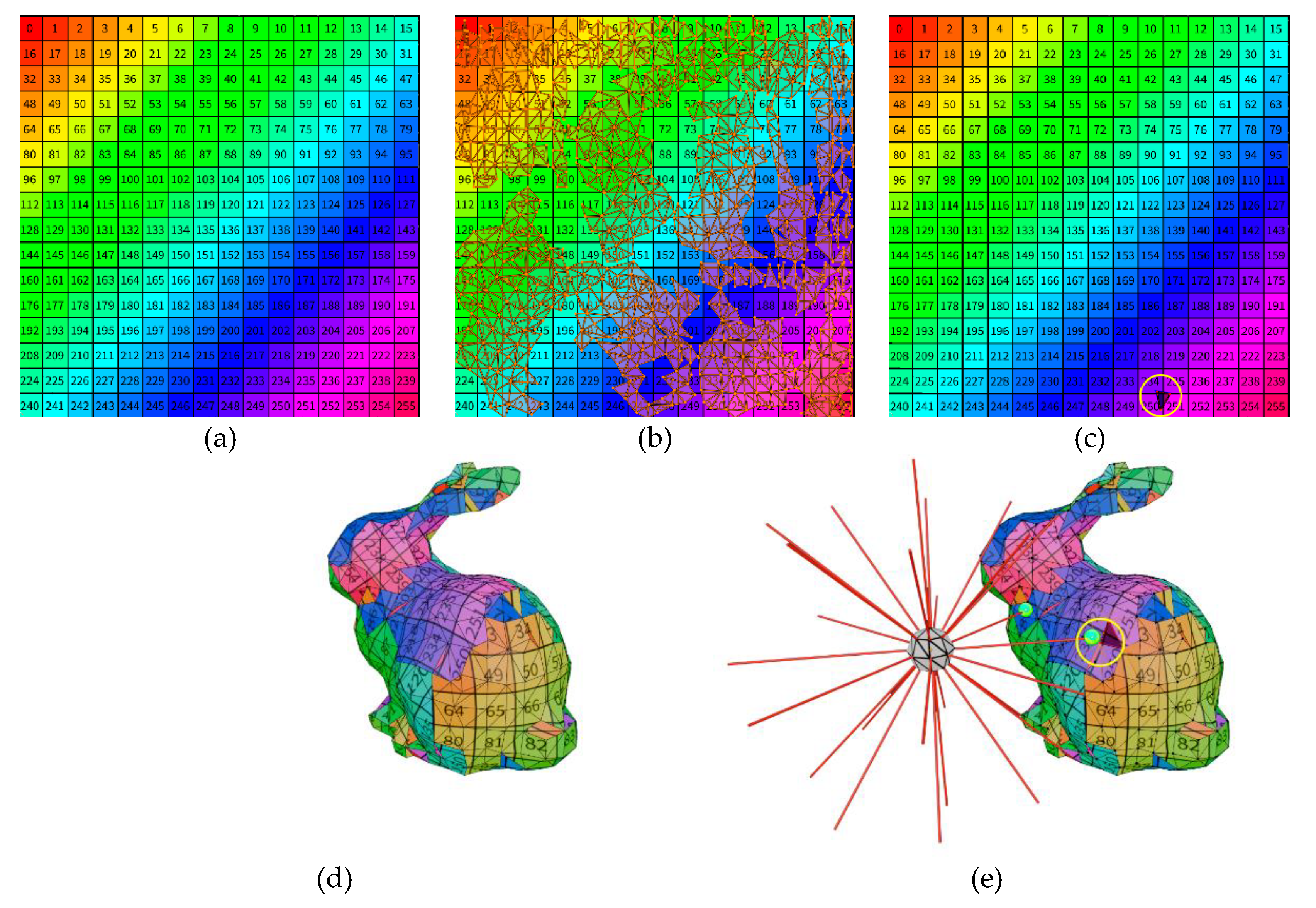
- Texture-based color: in this case, the user selects the texture image to be applied. To solve this color assignment, the UVMap property of scanned meshes is used. UVmap is a two-dimensional map, with U and V coordinates, that assigns the colors of a texture image to the vertices and faces of a mesh. For example, Figure 12d shows the texture mesh of a rabbit whose texture image is shown in Figure 12a. The UVmap, which creates a correspondence between the faces of the mesh displayed on the plane and the texture image, can be seen in Figure 12b. Since the texture mapping is only performed on the captured or scanned points (raycasting intersections), these points are taken and sampled in the Sample Nearest node, which is used to determine the closest point of the captured mesh to each scanned point, such as the point circled in yellow in Figure 12d. Then, using the Sample Index and Image Texture nodes, the UVMap coordinates of these points are determined, and thus the pixels to which they correspond in the texture image (Figure 12c), and this is the color assigned to each point.
Figure 12.
(a) Image texture applied to the mesh of (d); representation of the UVMAP with unwrapped mesh of (d) placed over the image texture of (a); (c) selection of the triangle intersected of (e) in the UVMAP; (d) textured mesh using the image of (a); (d) representation of the raycasting process of the scanner where the rays intersect the mesh and a correspondence between the intersection points and the pixels in the image texture can be established.
2.5.3. D representation.
The results of the scan simulation process can be visualized in several ways. The node tree that manages the rendering methods is shown in Figure 14.
Following the process described in the previous sections, the scanning process consists of projecting the points of a UV sphere onto the scanned mesh, composed of vertices, faces and normals. The vertex coordinates of the source sphere are transferred to the intersection points computed in Raycasting, but the definition of faces remains unchanged. Taking these starting data and considering the different input parameters of the add-on, the scheme shown in the Figure 15 is established. This scheme summarizes the different processes that are applied to these starting data, influenced by the input parameters and which give rise to three representation formats: point cloud, mesh and sparse points.
The default representation format is the point cloud, which is the format natively produced by laser scanners. This is achieved by removing the edges and faces information in the Mesh to Points node and then creating instances of a simple 3D model at each acquired point. The simple 3D model used is a UV sphere of three segments and two rings, which entails a small number of vertices and faces, allowing the number of elements to be represented in real time to be manageable when working with thousands of points. This number of elements is inversely proportional to the scanner input parameter ‘Angle’. It is up to the user to ensure that the selected angle is not too small, as this may hinder processing depending on the computer's specifications. At any time, the user can modify the radius of these spheres instantiated at each point.
Another representation method is the mesh, which preserves the topological relationships of the original sphere: edges and faces. The mesh corresponding to the scan consists of all the projected points and preserves the connection between them (edges and faces) of the UV sphere of the Scanner sphere. A flip-normal process must be applied to the resulting meshes, since normal vectors of the sphere are oriented outwards and those of the scanned meshes are oriented in the opposite direction. The number of faces in the mesh is inversely proportional to the scan angle. Figure 16b shows an example of this type of representation applied to the target mesh in Figure 16a. It is desirable to eliminate the connection between distant points that are likely to belong to different objects or regions of the mesh. To do this, the user has the option of removing edges from the mesh whose length exceeds a certain value. This value can be modified in real time until the resulting mesh meets the user's specifications, as shown in Figure 16c. This filtering is performed in the Filter Long Edges block. In this block, the geometric distances between each pair of mesh points are calculated and stored. The average value of these distances is then determined in the Attribute Statistics block. The filter value entered by the user is multiplied by this average value, resulting in the value δ. All edges whose length is greater than δ are removed. Thus, if the user enters a filter value of 2, edges with a length equal to or greater than twice the average length of all edges will be removed. Figure 16d depicts the result of the filtering applied to the mesh in Figure 16c.
Finally, to simulate the scanning process of other devices, such as lidar sensors, where the produced point cloud is not as linearly structured as laser scanners, the Sparse points option can be activated. In this case, the acquisition process introduces a randomness factor in point locations. This process is performed within the Sparse Points block. This mode of representation builds upon the mesh explained above, generating a random distribution of points across its surface. At these randomly distributed points, instances of individual UV spheres are created, as in the standard scanning process. using two parameters: Density, which defines the number of points per square meter, and Seed, which determines the randomness seed for point generation. Since this mode is based on the mesh, the edge filtering process described earlier also applies here. An example of this type of visualization is shown in Figure 16e.
2.3. Export Data
In addition to enabling real-time visualization of the scanning process within Blender, one of the most notable features of this add-on is its ability to export data for use in external software. Depending on the visualization mode chosen, it will be more appropriate to export in one format or another.
If a structured or sparse point representation mode has been selected, the Export to PLY function generates an ASCII PLY file containing the XYZ coordinates of the points, the associated RGB color, and the scalar value 'Hit Distance' which represents the distance of each point from the scanner. The RGB color corresponds to the color mode selected by the user, which can be a single color, color by distance or color by texture. In any case, regardless of the chosen color mode in which the PLY is saved, the 'Hit Distance' scalar is always included, enabling the visualization of point-to-scanner distances using alternative RGB scales in other software.
An additional export function has been implemented to export the scanning result of a scanner animation. That is, if the user creates an animation in Blender in which a scanner follows a defined path, a PLY file will be created with all the scans made in each frame. To manage point cloud density and avoid generating clouds with an excessive number of points, the possibility of specifying the start frame, the end frame and the step of the animation has been included. The resulting PLY file includes a scalar value that records the frame at which each point was generated. For example, Figure 17a illustrates the scanning of the corridor mesh in Figure 17b, using the translation animation of a single scanner with a frame step of 10. The point colors in the visualization represent the frame in which each point was acquired.
Conversely, if the mesh representation mode is selected, exporting should utilize Blender's native recording options found in the File → Export submenu. The most suitable formats for this purpose are OBJ or FBX, as they effectively preserve texture information.
Finally, a major functionality integrated into the design of this add-on is its role in assisting the planning of environmental scanning. For this purpose, the add-on includes features that display the height values of each scanner object introduced in the scene, along with the option of visualizing a scan map. This map is an image rendered from a zenithal point of view with an orthographic camera of a schematic visualization of the mesh to be scanned and a representation of the position of the scanners by means of red circles, with each circle indicating the height of the corresponding scanner.
3. Results
The final version of the add-on presented in this article is available to be downloaded in [33]. It includes the interfaces shown in Figure 19 to allow the user to control the variety of options explained above. A general interface is accessible from the 3D viewport tabs that allows the generation of as many scanner objects as desired associated to the selected target mesh (Figure 194). The combined PLY point cloud and the top view image can also be generated using this interface. Each scanner specific parameters and exportation options are accessible from the ‘Modifier’ menu (Figure 19b, c).
Several tests have been carried out with the developed add-on to prove its features. Some of them are described in the following paragraphs.
The set of target meshes used in these tests were obtained from various sources and were created by different methodologies. Those presented in this article are shown below.
- -
- Meshes acquired by laser scanners: Church of Santa Catalina in Badajoz.
- -
- -
- Meshes obtained by 3d modeling: City model [36]
- -
- Meshes acquired using iPad Pro (Lidar).
- -
- Digitized meshes using Matterport. House model from House Matterport repository [37].
We have simulated the process of scanning interiors of meshes of historical heritage buildings, such as the cases shown in Figure 20 (source: photogrammetry - Church of Santa María de Melque in Toledo [34]) and Figure 21 and Figure 22 (source: laser scanner - Church of Santa Catalina in Badajoz). Scan angles: 1.5 and 2.2, respectively, and range of 50 meters have been used in both examples.
The add-on has also been applied to scan the interior of conventional buildings. Figure 23 shows an example of scanning a house, acquired using a Matterport device. The particularity of this example is that instead of selecting a single target mesh, it is necessary to select all the meshes composing the building. To do this, the Blender 'Join' function is used to create a set of selected meshes, which results in a single element in the scene that combines all of them. Additionally, meshes digitized using the iPad Pro have been also used for testing TLSynth, as the examples shown in Figure 10, Figure 13 and Figure 17, in which a classroom, a laboratory and a long corridor were acquired, respectively.
These examples highlight the straightforwardness of the TLSynth application procedure for one of its primary functions: scan planning. As illustrated in Figure 24 , the process begins with a preliminary scan conducted using easily accessible devices, such as an iPad LiDAR or a Matterport camera, delivering a quick and low-resolution output. This initial result is then transferred to a computer, where TLSynth is utilized to evaluate, optimize, and plan the scanning process. A scan map (explained above) is subsequently generated to guide the technician in executing the high-resolution scanning campaign. Notably, this workflow enables the preliminary scan to be conducted remotely by a customer, who may be geographically distant from the technician responsible for the final scan, thereby significantly reducing unnecessary travel and associated costs.
Finally, additional tests have been conducted to demonstrate another use case: the simulation of digitization using laser scanners mounted on mobile vehicles. For this purpose, a single scanner is used, to which a motion animation is applied in Blender. Then, the add-on functionality is used to generate the point cloud resulting from the scanner animation. In the Figure 25 , the digitization of a city model obtained by 3D modeling [36], is shown. A linear movement has been applied to the scanner at ground level with an angle of and a minimum aperture of by means of an animation of 200 frames, simulating a car in motion with an on-board scanner. The resulting point cloud was generated by capturing data every 10 frames, with point colors corresponding to their respective animation frames.
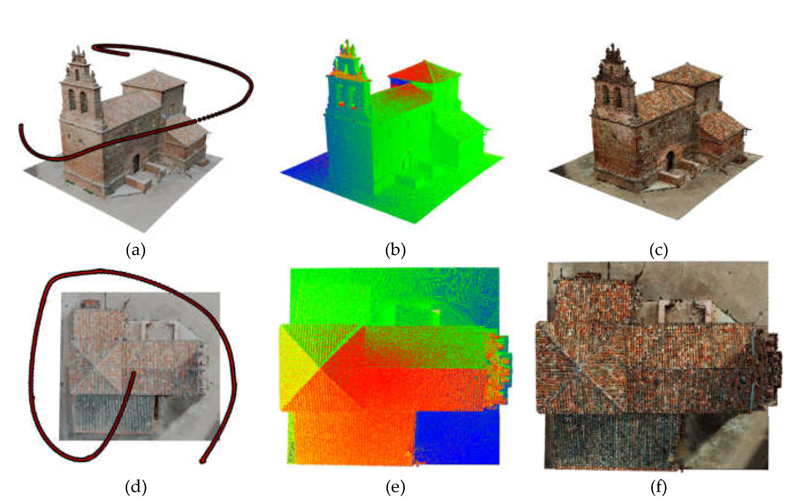
Similarly, Figure 26 depicts a simulation of digitization from a drone-mounted scanner. In this case, the 3D model of the Church of La Barbolla in Sigüenza [35], obtained by photogrammetry, was used as a target. An animation was created where the scanner followed the building's contour while gradually increasing its altitude. An angle of and an opening angle of was set. From the animation, a single point cloud was generated by capturing data every frame, with colors assigned according to the frame.
4. Discussion
This paper presents a laser scanner simulator developed as a blender add-on, TLSynth, that offers several notable advances over existing proposals, as discussed in the introduction. The most significant differences and improvements can be observed with regard to real-time functionality, parameter control, and export capabilities.
The primary advantage is its real-time functionality, which enables the immediate generation of synthetic point clouds. This feature distinguishes it from BlenSor [14], which, despite its popularity, lacks the capacity for real-time operations.
In addition, the proposed TLS simulator employs Blender's visual programming tools, facilitating real-time modifications of critical parameters such as scanner position, angle, resolution, and noise. This interactivity enhances the user's ability to optimize scanning configurations rapidly, which makes it particularly valuable for tasks such as performance optimization and site scan planning, where immediate feedback is essential. This feature distinguishes it from Gazebo [31], which offers LIDAR sensor simulations for robotic applications, but does not provide the fine-grained control over parameters and formats involved in high-precision terrestrial laser scanning.
A further noteworthy attribute of this proposal is its export functionality. The capacity to export data to common file formats, namely PLY, OBJ, and FBX, ensures seamless integration with other software used in the field of 3D modeling and point cloud processing. In particular, the PLY format is highly effective for storing point cloud data, as it captures both geometric and scalar information, including the XYZ coordinates, RGB color values, distance measurements or acquisition frame. Formats of this nature, wherein the cloud points feature supplementary attributes, are particularly advantageous for applications such as the one presented in [38,39], where our group developed a virtual reality tool to interactively explore and survey enriched point clouds. This feature also extends to the export of animation data, where the tool can generate a PLY file based on scans captured across multiple frames of a scanner's movement, offering an efficient method for creating large-scale point cloud datasets for algorithm testing and development.
It should also be noted, over the other alternatives, the possibility of generating mesh surfaces directly, in real time, which can be useful to generate data repositories for research, or the aleatory distribution on points over the mesh to simulate other types of 3D sensors.
The incorporation of scan planning tools serves to augment the functionality of the add-on. By providing a visual representation of the height of scanner objects and generating scan maps, the tool allows users to evaluate the efficacy of their scanning configuration. The scan map provides a top-down representation of the scanning environment, illustrating the positions of the scanners and identifying areas that may require additional scans. This feature is particularly useful for optimizing scan coverage and ensuring that essential elements of the scanned environment are captured with sufficient detail.
In terms of performance, the simulator generates synthetic point clouds that closely replicate those produced by real-world laser scanners. The inclusion of adjustable noise parameters serves to augment the realism of the tool, emulating real-world imperfections. This renders the tools a valuable asset not only for pre-scan planning but also for the generation of synthetic datasets applicable to machine learning and other domains. While BlenSor is an effective tool for generating synthetic datasets, such as SynthCity [16], it lacks the real-time interactivity offered by our simulator, which is essential for applications requiring rapid iterations and adjustments.
Notwithstanding the aforementioned strengths, the present implementation of the simulator is subject to certain limitations. To illustrate, the simulator does not currently provide users with real-time feedback on synthetic point clouds, beyond fundamental metrics such as position and point count. This limitation restricts the user's ability to fully evaluate the quality of the generated data throughout the simulation process. Additionally, an advanced user may perceive the level of interactivity to be inadequate. For instance, more precise control over the laser scanning behavior, such as the simulation of particular scanner settings (e.g., pulse rate, scan speed), may be required for applications requiring high precision. Another functionality that might be desirable would be the customization of the emitter geometry, currently based on a UV Sphere. Simpler shapes, could be considered, such as a sector of the sphere, with a vertical and a horizontal aperture angle, or as a simple circle, to simulate a 2D lidar.
Future research will focus on overcoming these limitations. One fundamental area of improvement is the full simulation of laser beam behavior, including interactions with different materials in the 3D environment model. This enhancement will allow the simulation to account for the effects of laser reflection, absorption, and scattering on a variety of surface types. Furthermore, an automatic reporting feature will be implemented, providing users with detailed information about each generated point cloud. It will include metrics such as the number of points, the average deviation, and the maximum deviation relative to the underlying 3D geometry.
Author Contributions
Conceptualization, A.S-H.; methodology, A.S-H., E.P. and P.M.; software, A.S-H. and E.P; validation, A.S-H. and E.P.; formal analysis, A.S-H. and E.P; investigation, A.S-H. and P.M; resources, A.S-H. and E.P; data curation, A.S-H. and E.P.; writing— original draft preparation, A.S-H. and P.M.; writing—review and editing, P.M and E.P.; supervision, P.M. and E.P.; project administration, P.M.; funding acquisition, P.M. All authors have read and agreed to the published version of the manuscript.
Funding
This research was funded by the Agencia Estatal de Investigación (Ministerio de Ciencia Innovación y Universidades) under Grant PID2019-108271RB-C32/AEI/10.13039/501100011033; and the Consejería de Economía, Ciencia y Agenda Digital (Junta de Extremadura) under Grant IB20172.
Data Availability Statement
The developed Blender add-on is available for download at https://github.com/3dcovim/TLSynth
Conflicts of Interest
The authors declare no conflicts of interest.
References
- B. Muralikrishnan, Performance evaluation of terrestrial laser scanners—a review, Meas. Sci. Technol. 32 (2021) 072001 (31pp), https://doi.org/10.1088/1361-6501/abdae3. [CrossRef]
- L. Ma, R. Sacks, R. Zeibak-Shini, A. Aryal, S. Filin, Preparation of synthetic as damaged models for post-earthquake BIM reconstruction research, J. Comput. Civ. Eng. 30 (2016) 1–12, https://doi.org/10.1061/(asce)cp.1943-5487.0000500. [CrossRef]
- Y. Xu, U. Stilla, Toward building and civil infrastructure reconstruction from point clouds: a review on data and key techniques, IEEE J. Select. Top. Appl. Earth Observat. Remot. Sens. 14 (2021) 2857–2885, https://doi.org/10.1109/JSTARS.2021.3060568. [CrossRef]
- Jong Won Ma, Thomas Czerniawski, Fernanda Leite, Semantic segmentation of point clouds of building interiors with deep learning: Augmenting training datasets with synthetic BIM-based point clouds, Automation in Construction, 2020, 113, 103144, https://doi.org/10.1016/j.autcon.2020.103144. [CrossRef]
- Autodesk Revit, Building information modeling software. https://www.autodesk.com/products/revit/overview.
- Trimble SketchUp, 3D modeling computer program. https://www.sketchup.com.
- Safe software fme, Data integration platform for spatial data. https://www.safe.com/fme/.
- Y. Jing, B. Sheil, S. Acikgoz, Segmentation of large-scale masonry arch bridge point clouds with a synthetic simulator and the BridgeNet neural network, Autom.Constr. 142 (2022), 104459, https://doi.org/10.1016/J.AUTCON.2022.104459. [CrossRef]
- Daniel Lamas, Andrés Justo, Mario Soilán, Belén Riveiro. Automated production of synthetic point clouds of truss bridges for semantic and instance segmentation using deep learning models. Automation in Construction, 2024, 158, 105176, https://doi.org/10.1016/j.autcon.2023.105176. [CrossRef]
- Q.-Y. Zhou, J. Park, V. Koltun, Open3D: A Modern Library for 3D Data Processing, 2018, https://doi.org/10.48550/arxiv.1801.09847. [CrossRef]
- M.C. Günes¸, A. Mertan, Y.H. Sahin, G. Unal, M. ¨Ozkar, Synthesizing Point Cloud Data Set for Historical Dome Systems, Communicat. Comput. Informat. Sci. 1465 CCIS (2022) 538–554, https://doi.org/10.1007/978-981-19-1280-1_33. [CrossRef]
- R. Zhai, J. Zou, Y. He, L. Meng, BIM-driven data augmentation method for semantic segmentation in superpoint-based deep learning network, Autom. Constr. 140 (2022), 104373, https://doi.org/10.1016/j.autcon.2022.104373. [CrossRef]
- L. T. De Paolis and P. Bourdot (Eds.): AVR 2019, LNCS 11613, pp. 203–219, 2019. https://doi.org/10.1007/978-3-030-25965-5_16. [CrossRef]
- BlenSor: Blender Sensor Simulation Toolbox M. Gschwandtner, R. Kwitt, A. Uhl In Advances in Visual Computing: 7th International Symposium, (ISVC 2011) Las Vegas, Nevada, USA, September 26 - 28, 2011.
- Blender, Open source 3D Creation Suite. blender.org, 2024 (last access: 10.08.2023).
- D. Griffiths, J. Boehm, SynthCity: a large scale synthetic point cloud, arXiv preprint, 2019, https://doi.org/10.48550/arXiv.1907.04758. [CrossRef]
- Wu, A. Wan, X. Yue, K. Keutzer, Squeezeseg: Convolutional neural nets with recurrent crf for real-time road-object segmentation from 3d lidar point cloud. IEEE International Conference on Robotics and Automation (ICRA), IEEE, May 2018, 1887–1893, https://doi.org/10.1109/ICRA.2018.8462926. [CrossRef]
- B. Wu, X. Zhou, S. Zhao, X. Yue, K. Keutzer, Squeezesegv2: Improved model structure and unsupervised domain adaptation for road-object segmentation from a lidar point cloud. International Conference on Robotics and Automation (ICRA), IEEE, May 2019, 4376–4382, https://doi.org/10.1109/ICRA.2019.8793495. [CrossRef]
- J. Fang, D. Zhou, F. Yan, T. Zhao, F. Zhang, Y. Ma, R. Yang, Augmented lidar simulator for autonomous driving, IEEE Robot. Auto. Lett. 5 (2) (2020) 1931–1938, https://doi.org/10.1109/LRA.2020.2969927. [CrossRef]
- J.W. Ma, B. Han, F. Leite, An Automated Framework for Generating Synthetic Point Clouds from as-Built BIM with Semantic Annotation for Scan-to-BIM. Proceedings - Winter Simulation Conference 2021-Decem, 2021, https://doi.org/10.1109/WSC52266.2021.9715301. [CrossRef]
- B. Han, J.W. Ma, F. Leite, A framework for semi-automatically identifying fully occluded objects in 3D models: towards comprehensive construction design review in virtual reality, Adv. Eng. Inform. 50 (2021), 101398, https://doi.org/10.1016/j.aei.2021.101398. [CrossRef]
- Kamil Korus, Thomas Czerniawski, Marek Salamak. Visual programming simulator for producing realistic labeled point clouds from digital infrastructure models. Automation in Construction, 2023, 156,105126, https://doi.org/10.1016/j.autcon.2023.105126. [CrossRef]
- Dynamo, Open Source Graphical Programming for Design. github.com/DynamoDS/Dynamo, 2023.
- Lukas Winiwarter, Alberto Manuel Esmorís Pena, Hannah Weiser, Katharina Anders, Jorge Martínez Sánchez, Mark Searle, Bernhard Höfle. Virtual laser scanning with HELIOS++: A novel take on ray tracing-based simulation of topographic full-waveform 3D laser scanning. Remote Sensing of Environment, 2022, 269,112772, https://doi.org/10.1016/j.rse.2021.112772. [CrossRef]
- F. Noichl, A. Braun, A. Borrmann, “BIM-to-Scan” for Scan-to-BIM: Generating Realistic Synthetic Ground Truth Point Clouds based on Industrial 3D Models. Proceedings of the 2021 European Conference on Computing in Construction 2, 2021, 164–172, https://doi.org/10.35490/ec3.2021.166. [CrossRef]
- V. Zahs, K. Anders, J. Kohns, A. Stark, B. H¨ofle, Classification of structural building damage grades from multi-temporal photogrammetric point clouds using a machine learning model trained on virtual laser scanning data, Int. J. Appl. Earth Obs. Geoinf. 122 (2023), 103406, https://doi.org/10.1016/j.jag.2023.103406. [CrossRef]
- CARLA, Simulator. https://carla.org/, 2023 (accessed July 11, 2024).
- F. Wang, Y. Zhuang, H. Gu, H. Hu, Automatic generation of synthetic LiDAR point clouds for 3-D data analysis, IEEE Trans. Instrum. Meas. 68 (2019) 2671–2673, https://doi.org/10.1109/TIM.2019.2906416. [CrossRef]
- J.E. Deschaud, D. Duque, J.P. Richa, S. Velasco-Forero, B. Marcotegui, F. Goulette. Paris-CARLA-3D: a real and synthetic outdoor point cloud dataset for challenging tasks in 3D mapping, Remote Sens. 13 (2021) 4713, https://doi.org/10.3390/RS13224713. [CrossRef]
- MORSE: Modular Open Robots Simulator Engine. https://morse-simulator.github.io/. (accessed July 11, 2024).
- Gazebo, Robotic Design, Development and Simulation Suite. gazebosim.org, (accessed July 11, 2024).
- VRscan3D. A simulator for terrestrial laser scanning in virtual reality. http://www.vrscan3d.com/. (accessed July 11, 2024).
- TLSynth Github Available online: https://github.com/3dcovim/TLSynth.
- Global Digital Heritage and GDH-Afrika. Available for download at https://sketchfab.com/3d-models/santa-maria-de-melque-toledo-spain-36cacabf9f364f8cbd45ff659a6144d4.
- Global Digital Heritage and GDH-Afrika. Available for download at https://sketchfab.com/3d-models/la-barbolla-church-siguenza-spain-dacdc9a91c33440780063e7a69f43bd3.
- Full Gameready City Buildings Available online: https://sketchfab.com/3d-models/full-gameready-city-buildings-0545317292c44490af5408cb58633121.
- Chang, A.; Dai, A.; Funkhouser, T.; Halber, M.; Niebner, M.; Savva, M.; Song, S.; Zeng, A.; Zhang, Y. Matterport3D: Learning from RGB-D Data in Indoor Environments. In Proceedings of the 2017 International Conference on 3D Vision (3DV); IEEE, 2017; pp. 667–676.
- Pérez, E.; Merchán, P.; Espacio, A.; Salamanca, S. Fusion of Thermal Point Cloud Series of Buildings for Inspection in Virtual Reality. Buildings 2024, 14, 2127, doi:10.3390/buildings14072127. [CrossRef]
- VR Point Cloud Analysis Github Available online: https://github.com/3dcovim/VR-Point-Cloud-Analysis.
Figure 1.
Blender interface in the Geometry Nodes workspace.
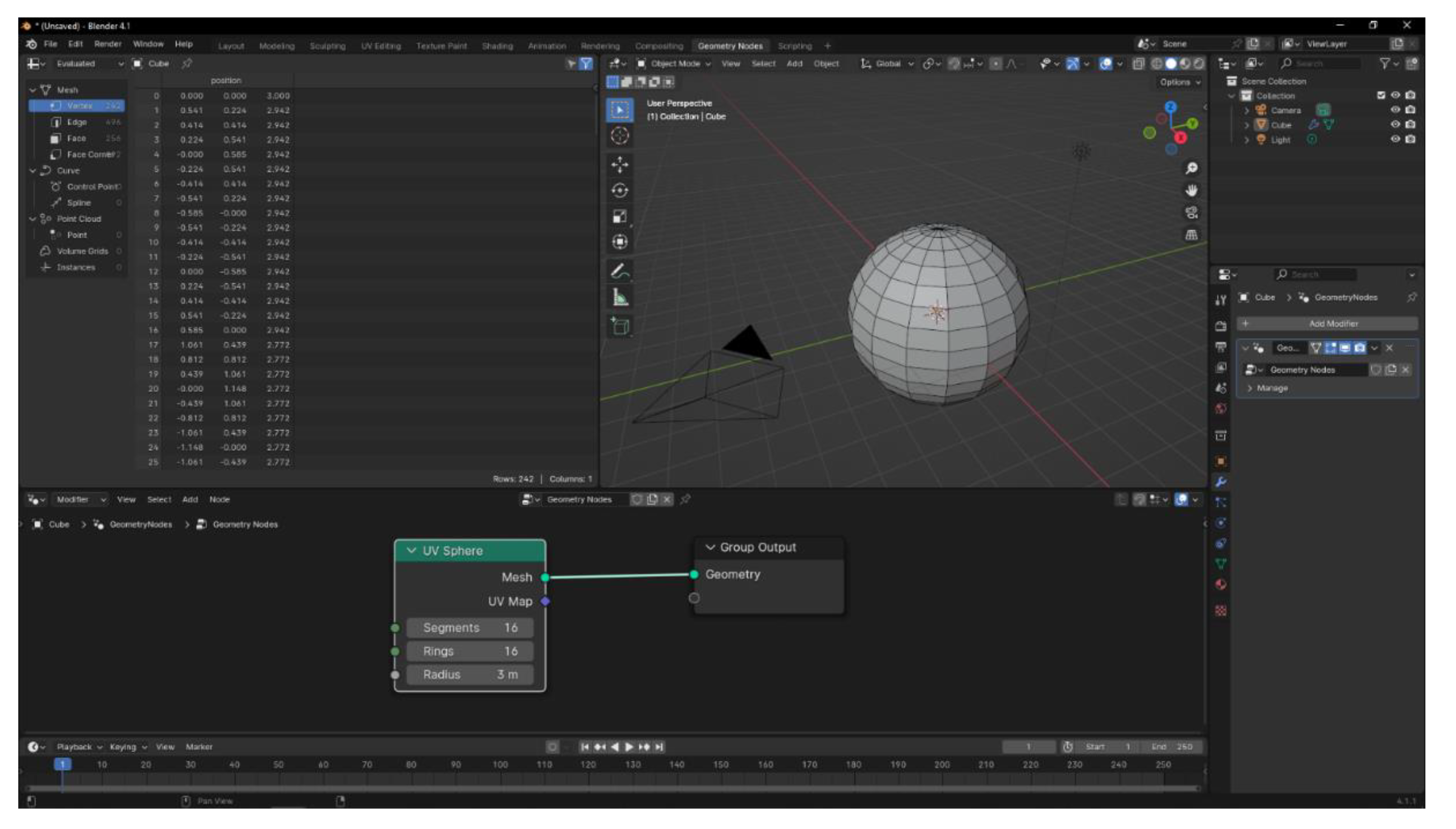
Figure 2.
Geometry Nodes tree that is integrated in every scanner object.

Figure 3.
TLSynth add-on general schema.
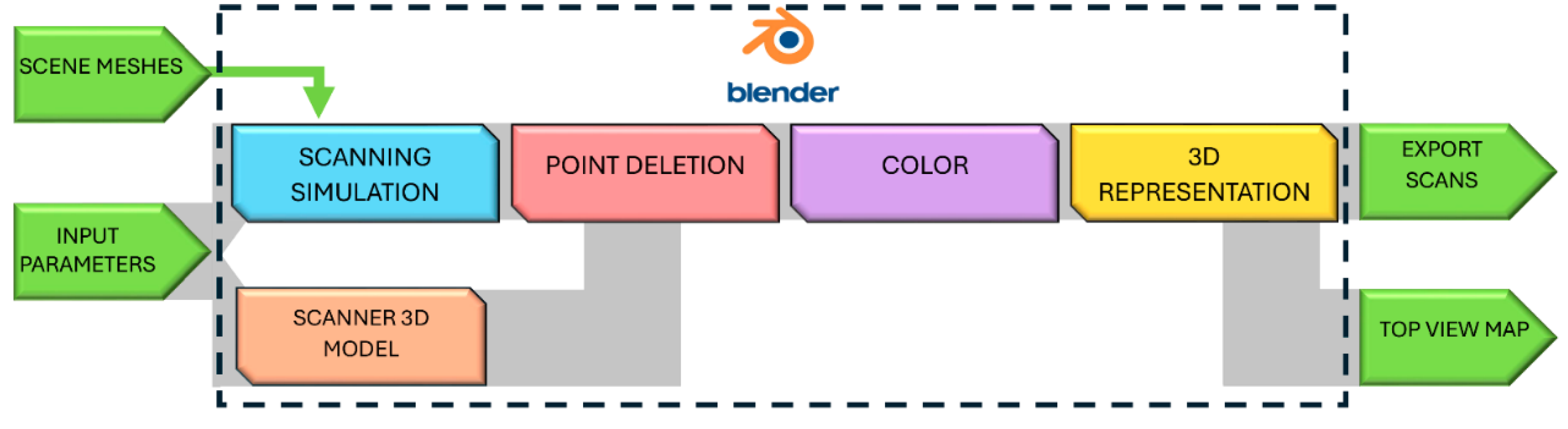
Figure 4.
Geometry Nodes tree associated to the ‘Scanner’ block.
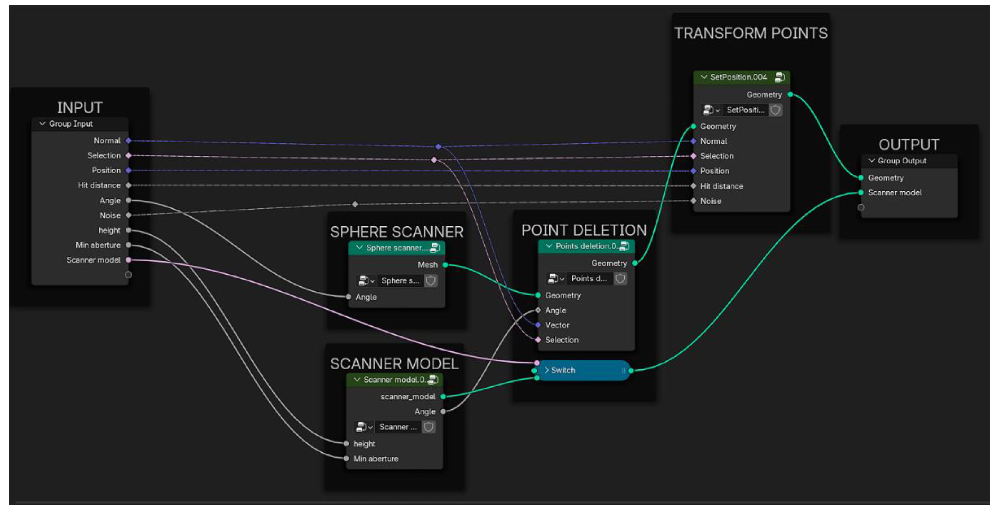
Figure 5.
(a) UV Sphere on which the scanning simulation process is based; (b) and (c) rings and segments, respectively, which can be defined in the UV Sphere node; (d), (e) and (f) vertices, normal on vertices and rays defined by both of them, respectively, that produce the scanning simulation; (g) graphical explanation of the parameters – range and angle – that user can set for each scanner object, that are related to the generated rays.
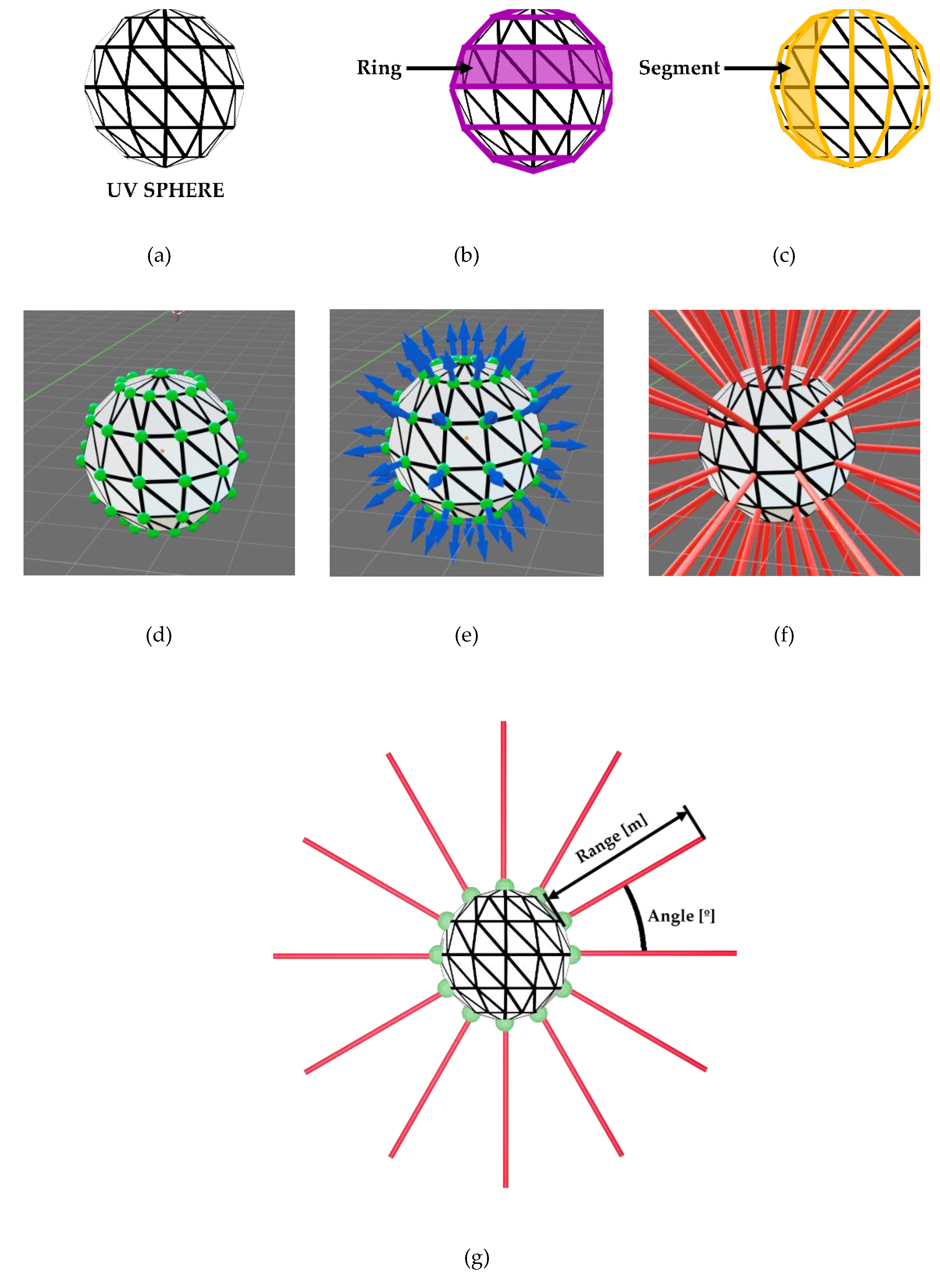
Figure 6.
Geometry Nodes tree associated to the ‘Raycasting’ block.
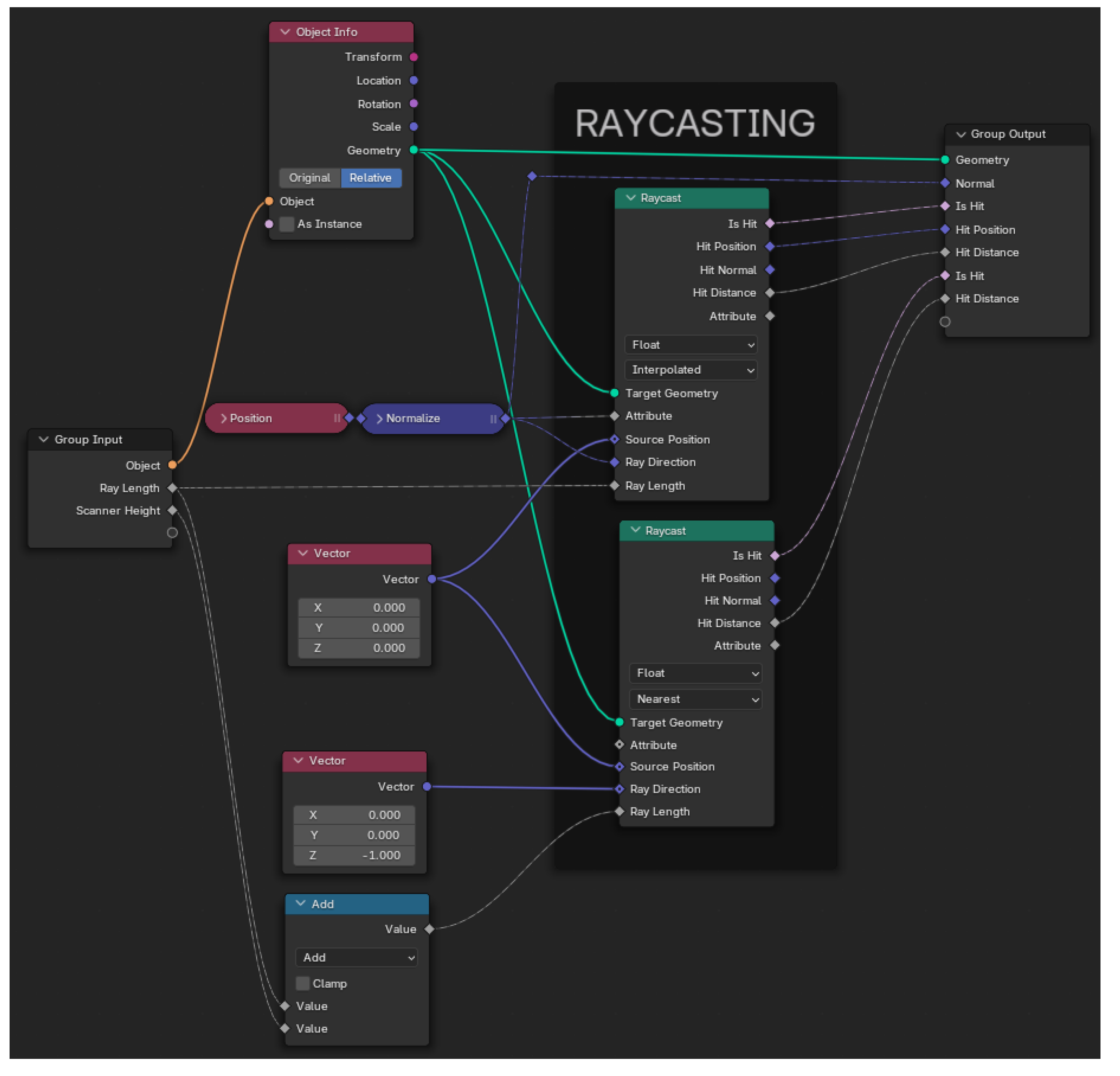
Figure 10.
(a) Example of target mesh of a classroom; (b) Result of the scanner simulation using three scanners with different minimum aperture parameters and their scanner models activated.
Figure 10.
(a) Example of target mesh of a classroom; (b) Result of the scanner simulation using three scanners with different minimum aperture parameters and their scanner models activated.
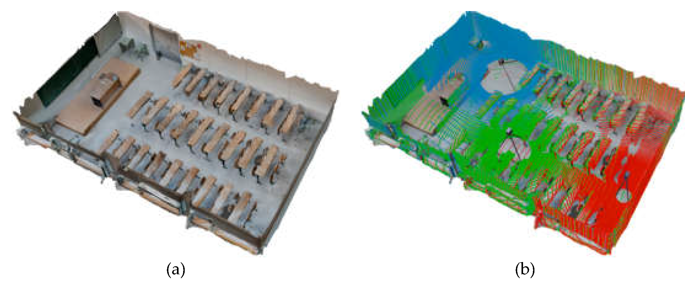
Figure 11.
Geometry Nodes tree associated to the ‘Color block.
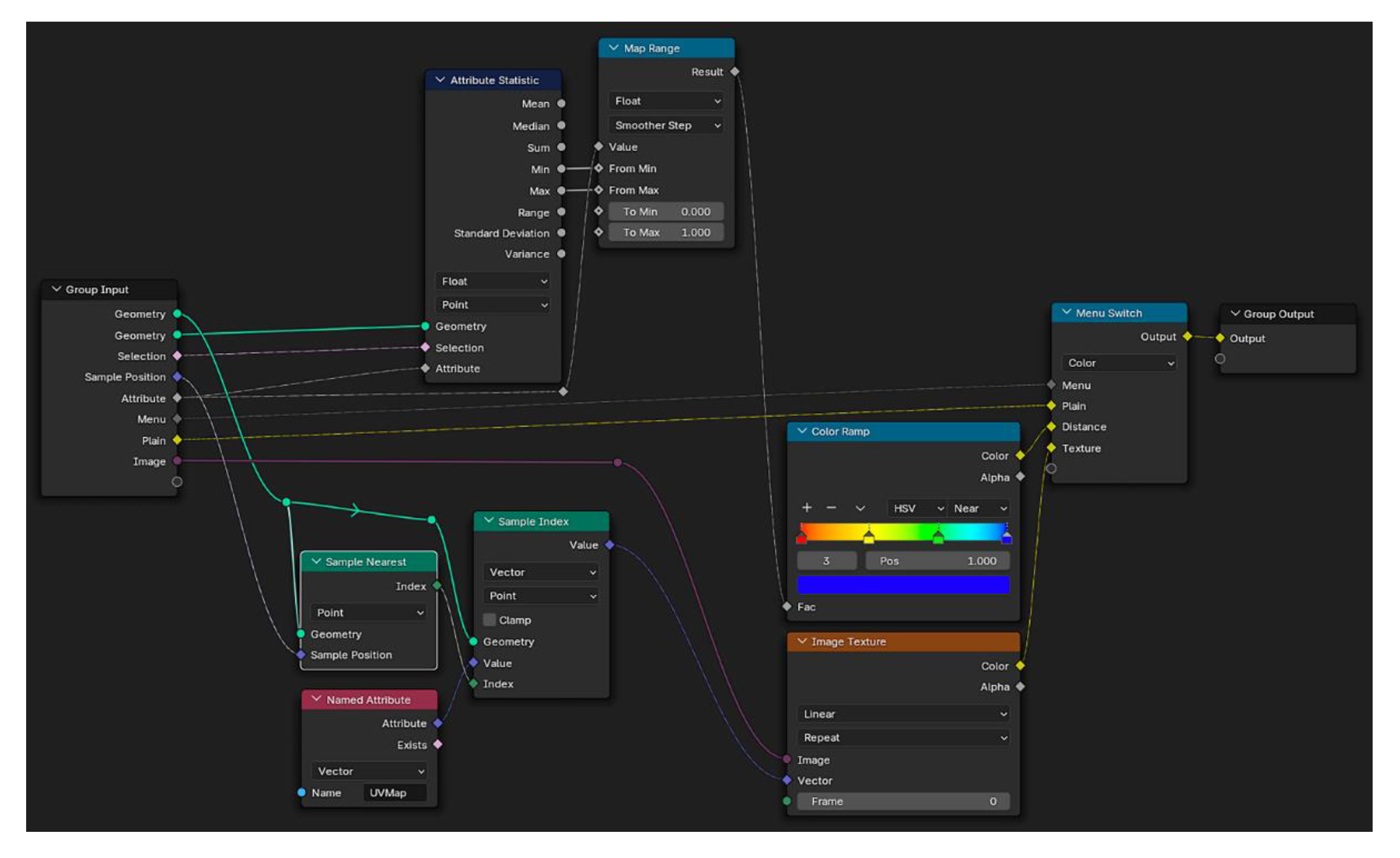
Figure 13.
Examples of the three alternatives for the color assignment to the resulting data (point cloud or mesh) of the scanning process: (a) solid color; (b) color based on the distance to the scanner; (c) color based on the image texture pixel associated to each point.
Figure 13.
Examples of the three alternatives for the color assignment to the resulting data (point cloud or mesh) of the scanning process: (a) solid color; (b) color based on the distance to the scanner; (c) color based on the image texture pixel associated to each point.
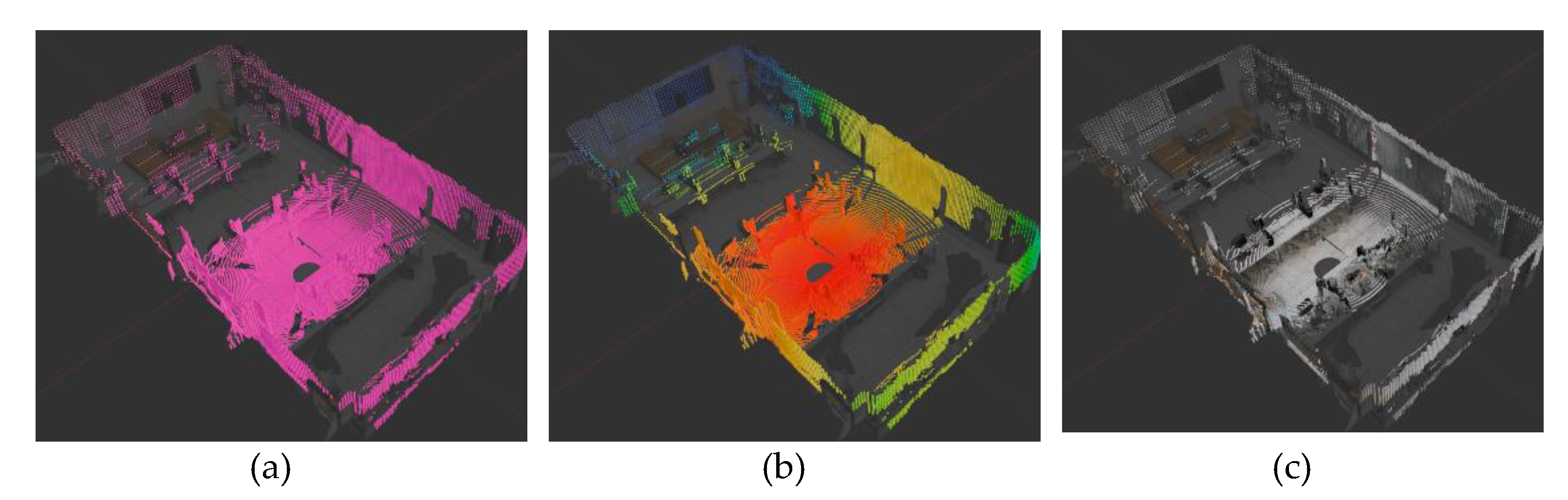
Figure 14.
Geometry Nodes tree associated to the ‘3D representation’ block.
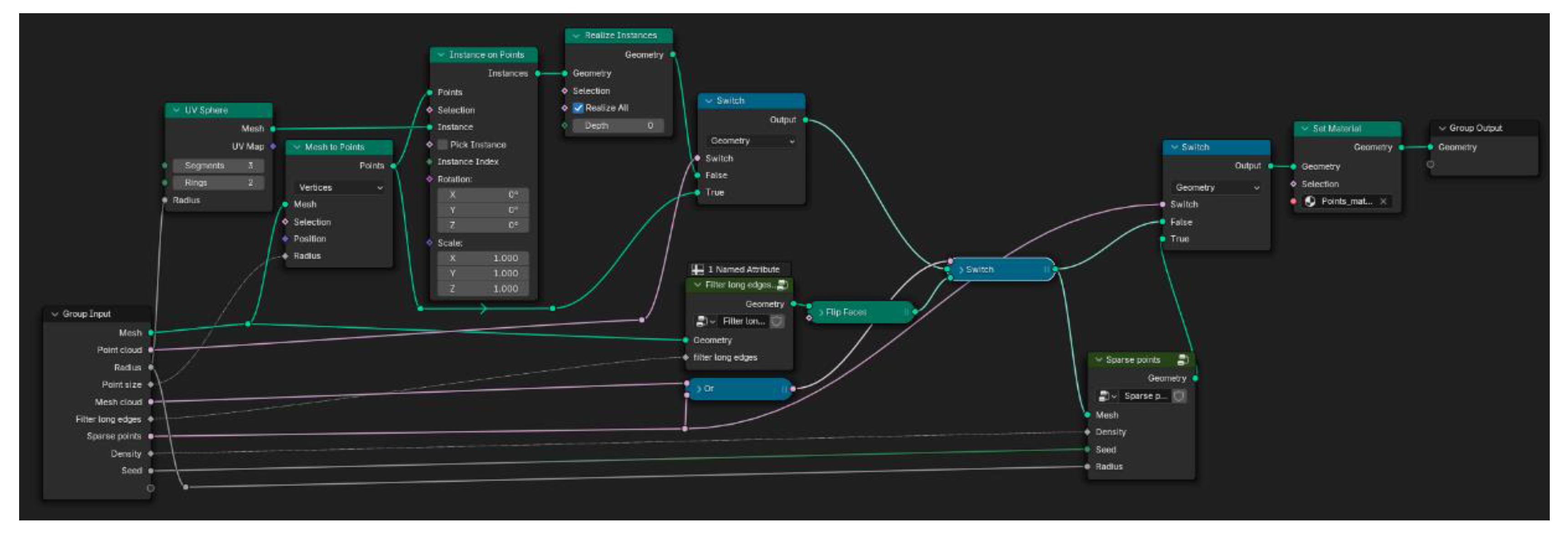
Figure 15.
Schema of the processes applied to the source data (vertices, faces and normal of the UV Sphere) and affected by the input parameters.
Figure 15.
Schema of the processes applied to the source data (vertices, faces and normal of the UV Sphere) and affected by the input parameters.
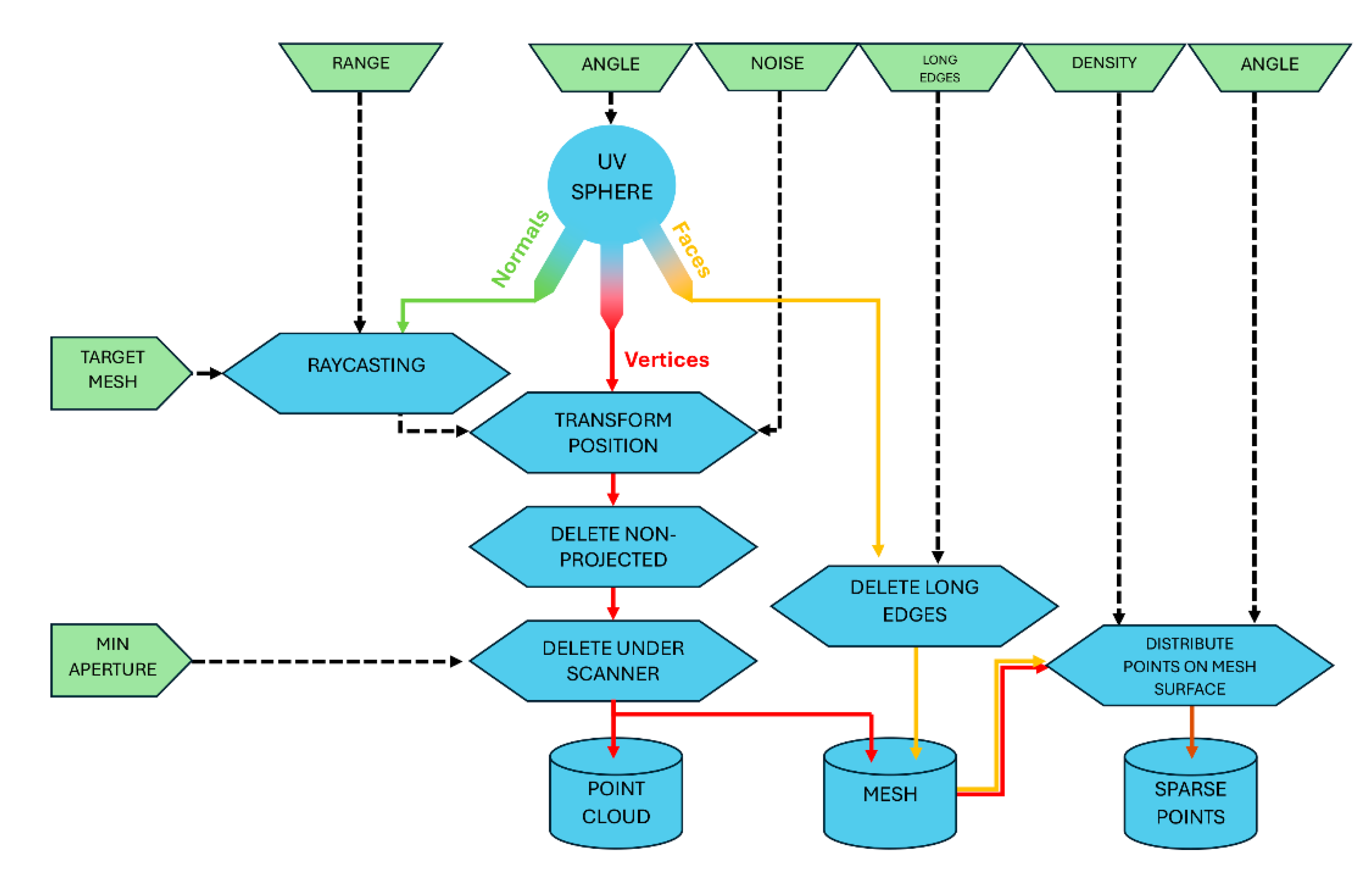
Figure 16.
Examples of the three alternatives for the representation of the resulting data of the scanning process, using the color based on the image texture: (a) Target mesh which has been scanned; (b) resulting point cloud; (c) resulting mesh without any filter; (d) resulting mesh with a filter applied to long edges; (e) resulting sparse points based on the aleatory distribution of points over the computed mesh.
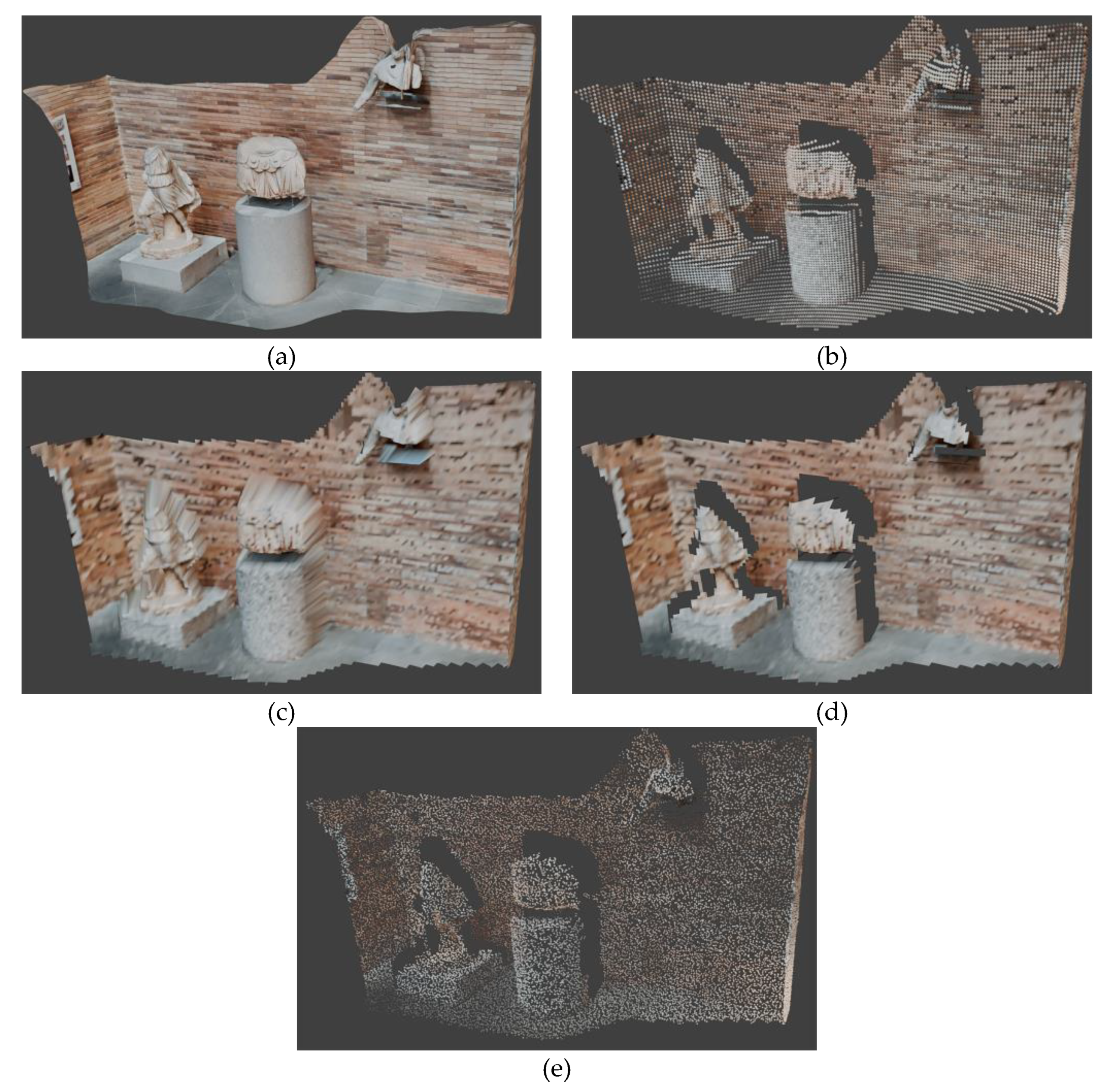
Figure 17.
Example of generation of PLY file from the animation of a single scanner’s movement: (a) Target mesh which has been scanned; (b) resulting mesh of the scanning process produced after animating the scanner with a linear translation along frames and with a step frame of .
Figure 17.
Example of generation of PLY file from the animation of a single scanner’s movement: (a) Target mesh which has been scanned; (b) resulting mesh of the scanning process produced after animating the scanner with a linear translation along frames and with a step frame of .
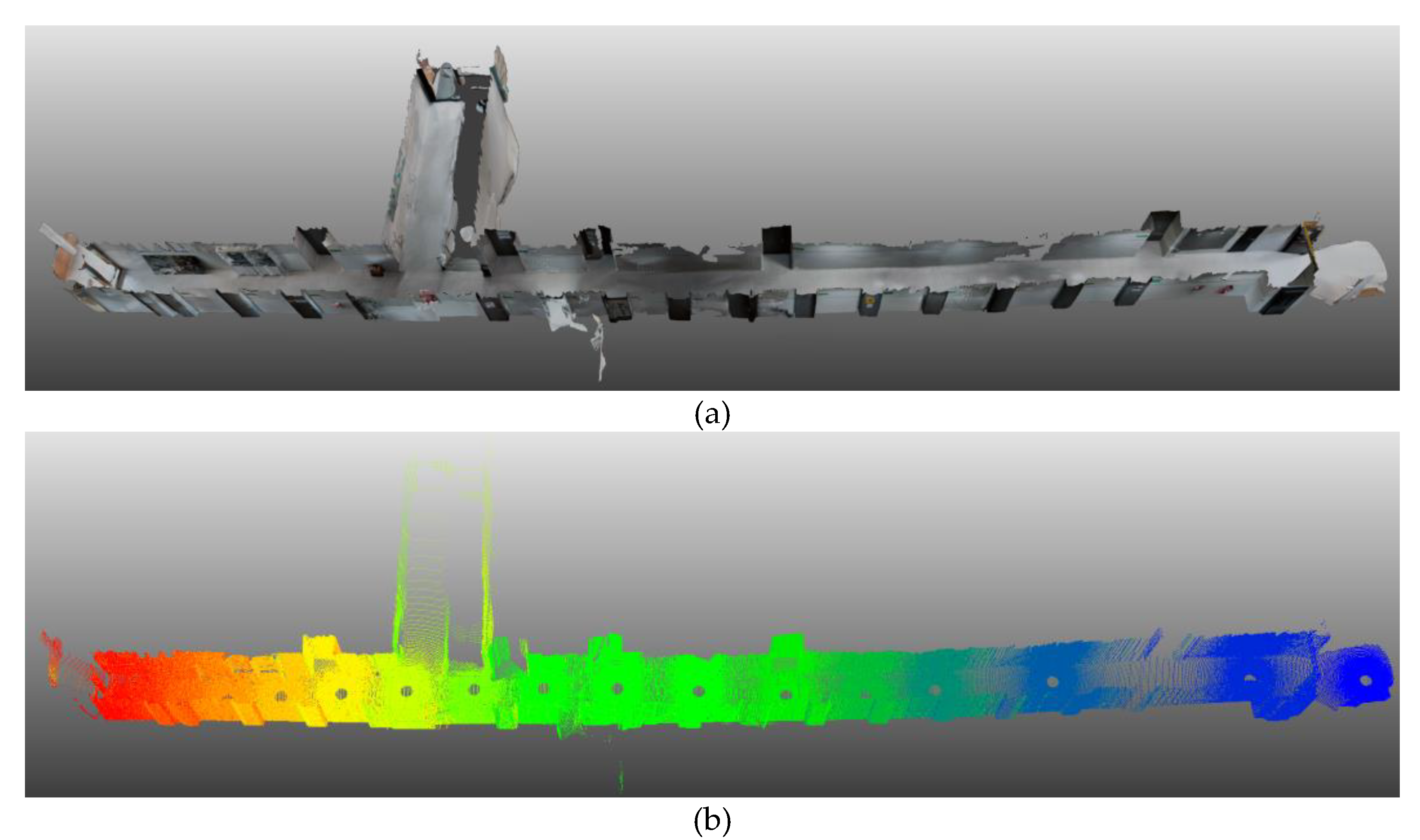
Figure 18.
Top view map example of the scanning simulation with the three scanners depicted in Figure 10. A simple wireframe representation is applied to the target mesh and each scanner is represented by a circle containing the value of its height with respect to the floor.
Figure 18.
Top view map example of the scanning simulation with the three scanners depicted in Figure 10. A simple wireframe representation is applied to the target mesh and each scanner is represented by a circle containing the value of its height with respect to the floor.
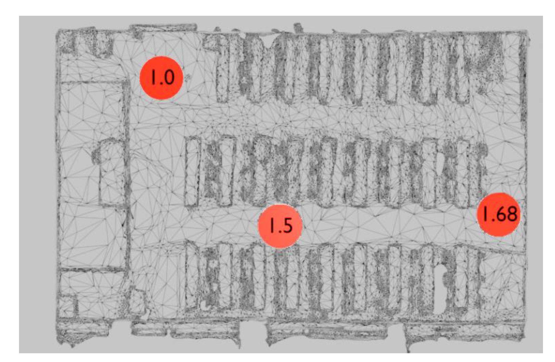
Figure 19.
User interfaces included in the TLSynth add on: (a) General interface accessible from the 3D viewport tabs; (b) and (c) scanner interfaces accessible from the modifier menu in each scanner object.
Figure 19.
User interfaces included in the TLSynth add on: (a) General interface accessible from the 3D viewport tabs; (b) and (c) scanner interfaces accessible from the modifier menu in each scanner object.
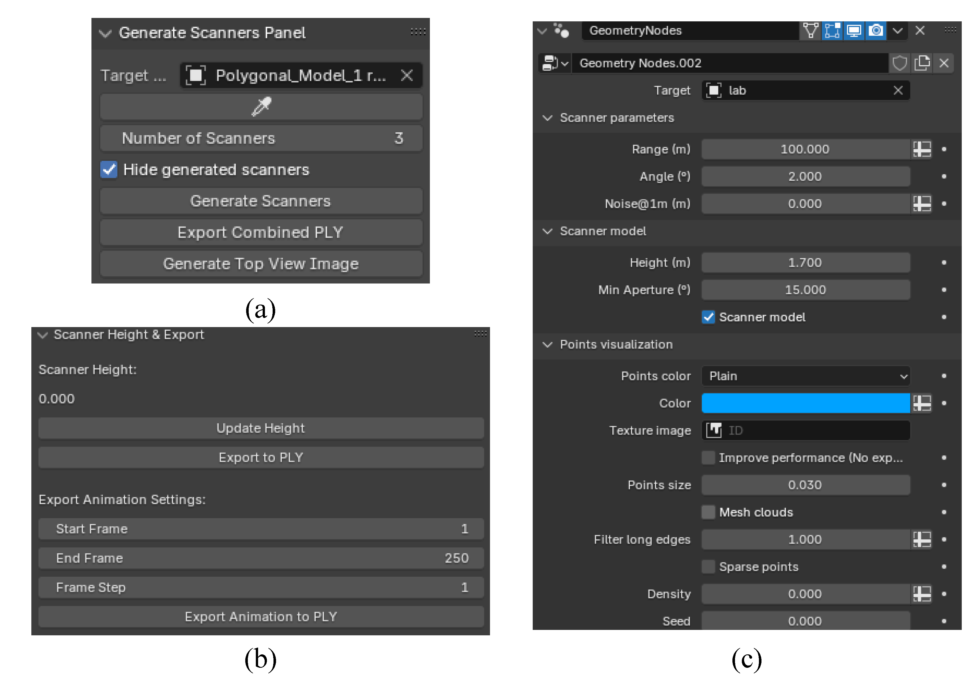
Figure 20.
Scanning simulation ( scans; angle ; range m) of the interior of the interior of a Cultural Heritage building: source photogrammetry - Church of Santa María de Melque in Toledo [33]: (a) and (b) perspective and section views of the initial 3D model, respectively; (c) interior view of the building; (d) scanning of the interior; (e) resulting point cloud with three colors, one for each of the scans.
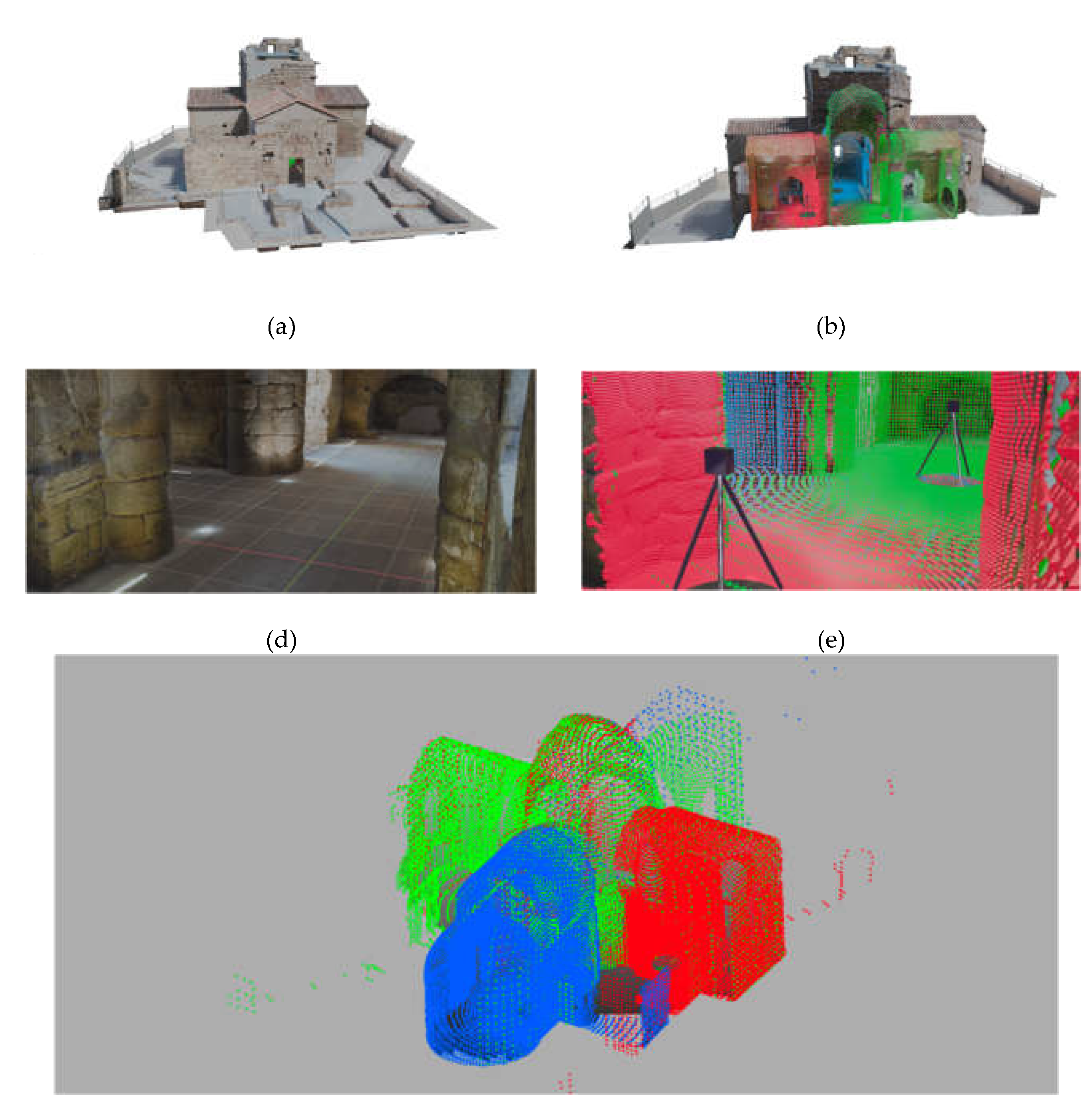
Figure 21.
Resulting point clouds of scanning simulation ( scans; angle ; range m) of the interior of a Cultural Heritage building: source laser scanner - Church of Santa Catalina in Badajoz.
Figure 21.
Resulting point clouds of scanning simulation ( scans; angle ; range m) of the interior of a Cultural Heritage building: source laser scanner - Church of Santa Catalina in Badajoz.
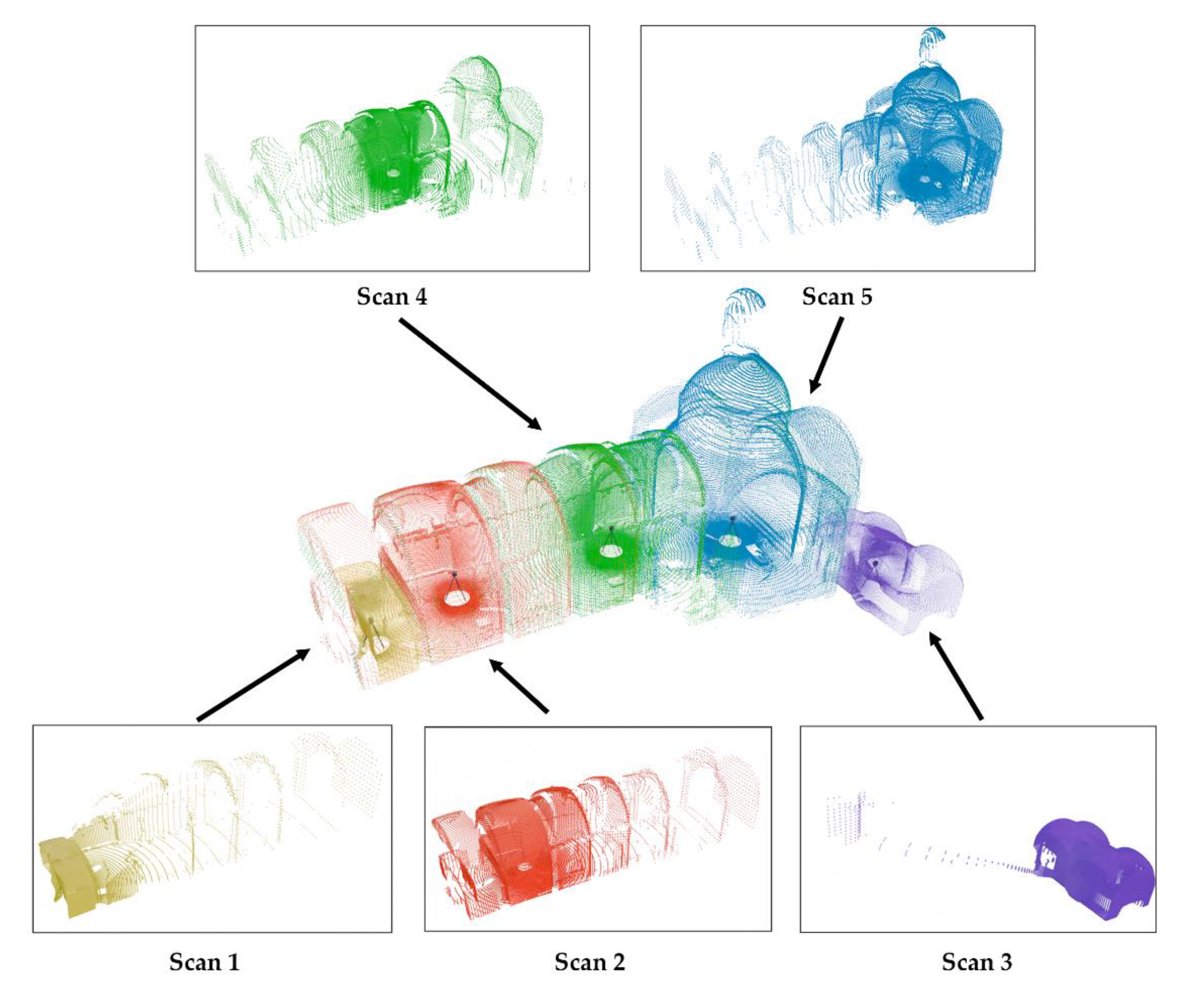
Figure 22.
Comparison between the original target mesh (a) of the building used for the scanning in Figure 21 and the generated mesh cloud (b) after the scanning process.
Figure 22.
Comparison between the original target mesh (a) of the building used for the scanning in Figure 21 and the generated mesh cloud (b) after the scanning process.
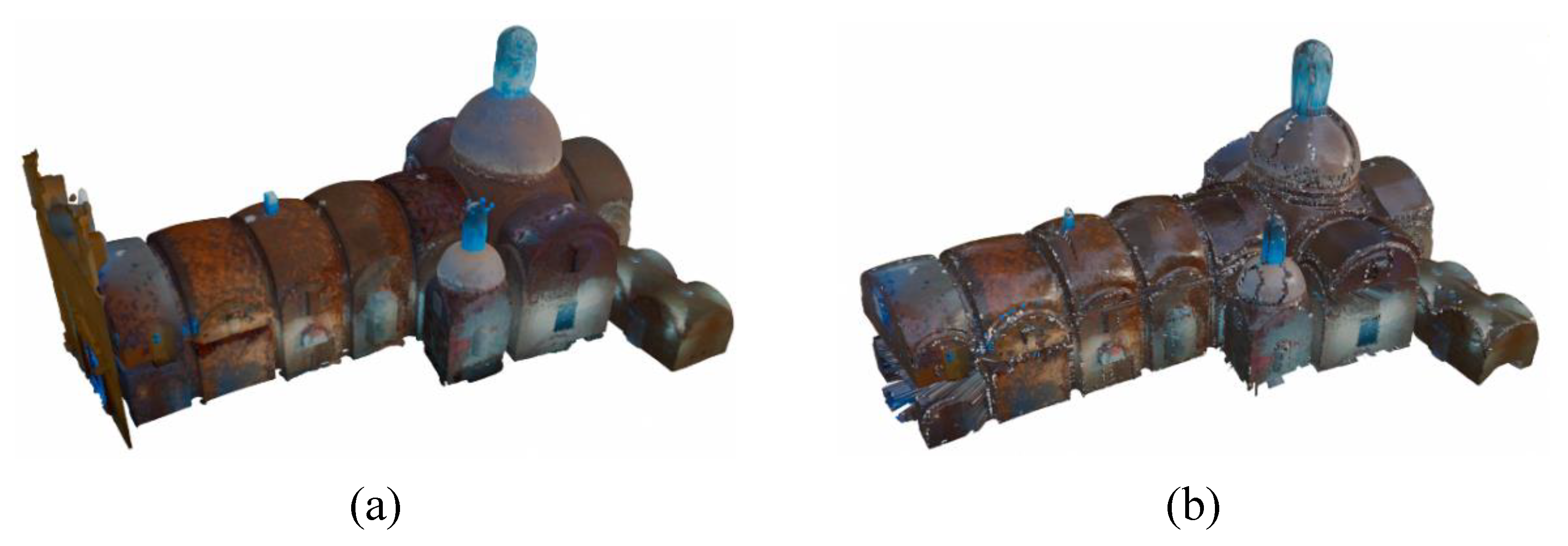
Figure 23.
Scanning simulation ( scans; angle range m) of the interior of a conventional house: source Matteport - House model from House Matterport repository [3]: (a) original set of meshes for every room of the house; (b) registered set of meshes; (c) resulting point clouds of the scanning of a set of target meshes, with nine colors, one for each of the scans.
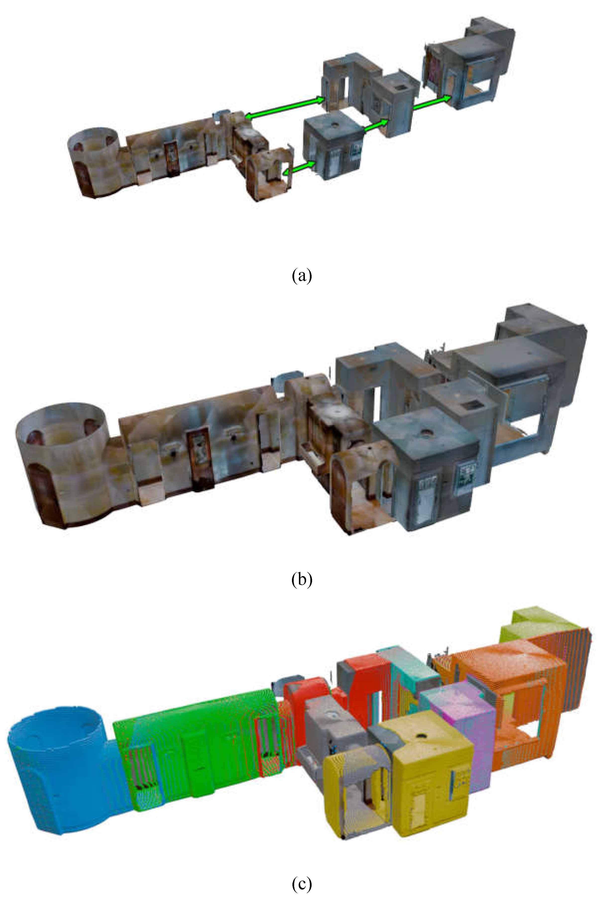
Figure 24.
Proposed workflow of the use of TLSynth for planning laser scanners campaigns.
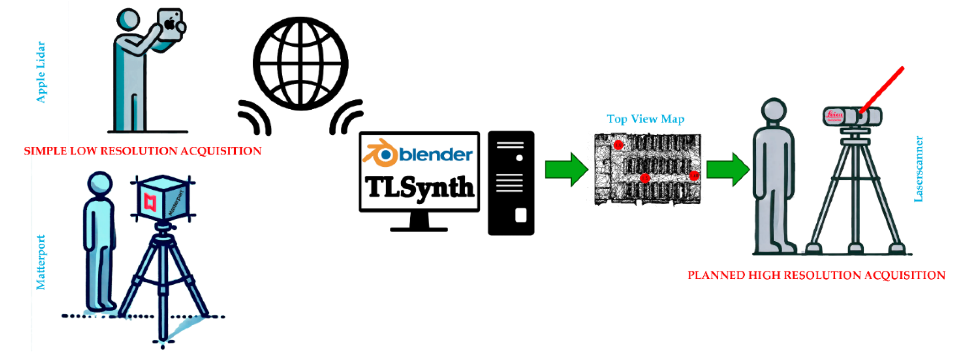
Figure 25.
Scanning simulation (20 scans; angle ; range 80 m) of a city model: source 3D modelling [36]: (a) original modeled mesh; (b) four instants of the animation with colored point clouds based on distance; (c) and (d) different views of the resulting point cloud obtained from the animation sequence, using a frame step of 10 frames. The colors are associated in terms of the scanning frame.
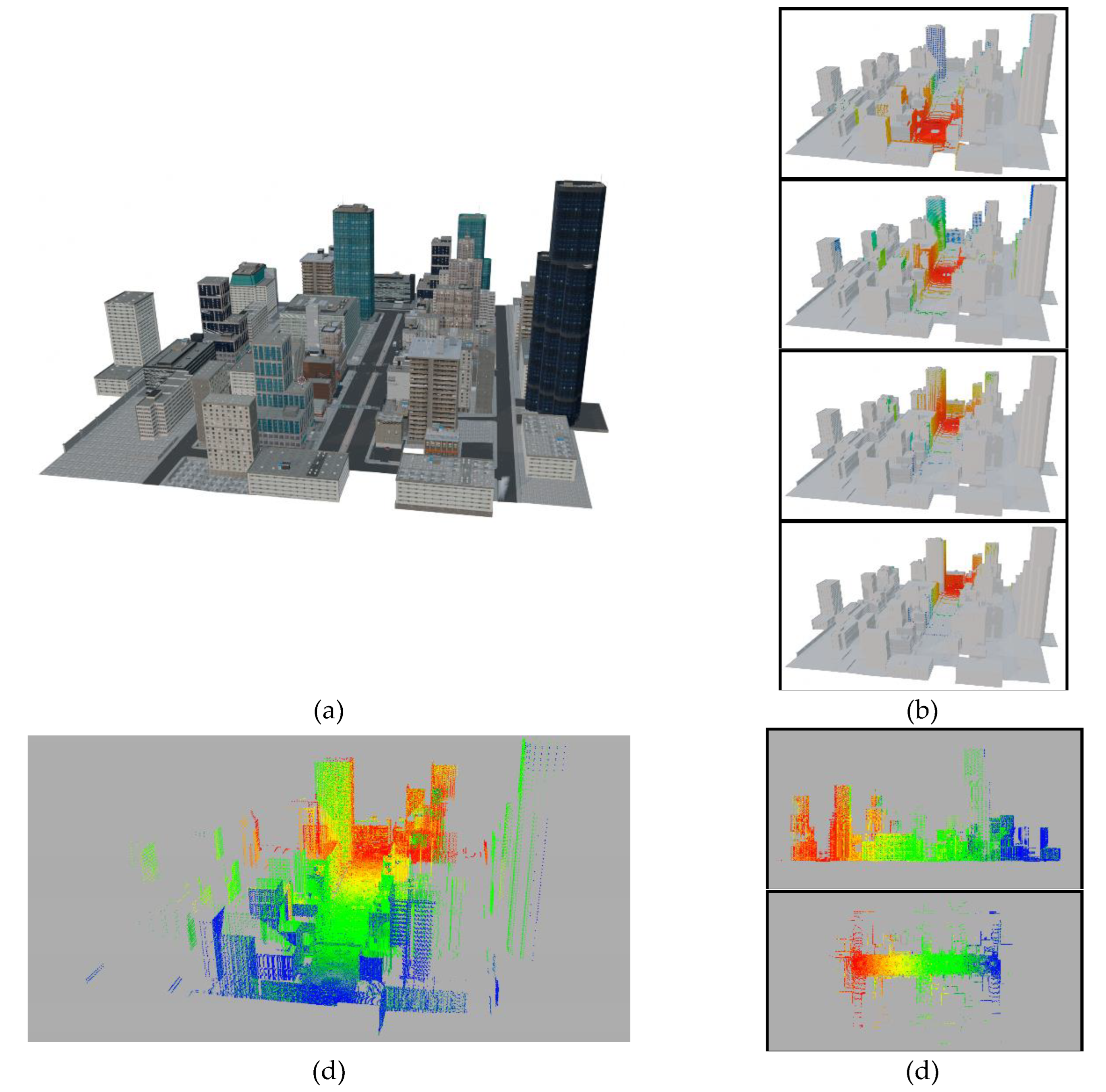
Figure 26.
Scanning simulation ( scans; angle ; range m) of the interior of a Cultural Heritage building: source photogrammetry - Church of La Barbolla in Sigüenza [34]: (a) and (d) perspective and top view of the original 3D mesh with the scanner animation path; (b) and (e) perspective and top view of the resulting point cloud after the animation; (c) and (f) perspective and top view of the resulting point cloud with color assignation based on the original texture of the target mesh.
Disclaimer/Publisher’s Note: The statements, opinions and data contained in all publications are solely those of the individual author(s) and contributor(s) and not of MDPI and/or the editor(s). MDPI and/or the editor(s) disclaim responsibility for any injury to people or property resulting from any ideas, methods, instructions or products referred to in the content. |
© 2024 by the authors. Licensee MDPI, Basel, Switzerland. This article is an open access article distributed under the terms and conditions of the Creative Commons Attribution (CC BY) license (http://creativecommons.org/licenses/by/4.0/).
Copyright: This open access article is published under a Creative Commons CC BY 4.0 license, which permit the free download, distribution, and reuse, provided that the author and preprint are cited in any reuse.


