Submitted:
02 September 2025
Posted:
03 September 2025
You are already at the latest version
Abstract
It is of great significance to construct a networked energy-saving driving strategy method and application framework to solve the problems of traffic disorder, speed fluctuations, and high energy consumption caused by frequent acceleration, deceleration, and lane changing of vehicles in road sections with variable traffic flow. Considering the mixed traffic scenario where autonomous vehicles and manually driven vehicles interact and infiltrate, a hybrid traffic flow vehicle energy-saving driving model was established, and the Dueling Double Deep Q-Network (D3QN) was used to optimize and solve the energy-saving driving model; Selecting Qingdao urban intersections as application scenarios, energy-saving driving strategy application facilities were constructed in simulation experiments to carry out simulation verification of energy-saving driving strategies for mixed traffic flow in the context of vehicle networking. The simulation results show that in different scenarios with different proportions of CAVs, the energy-saving strategy based on D3QN deep reinforcement learning algorithm can achieve fuel savings of 8.41%~6.67% compared to conventional strategies. Compared with the ordinary reinforcement learning algorithm Q-learning, its fuel saving rate is increased by 1.94%~1.5%, and the energy-saving effect becomes more significant with the increase of traffic density; From the perspective of dynamic characteristics, the speed stability under the control of D3QN algorithm is superior to Q-learning algorithm, and significantly better than conventional strategies, further highlighting the comprehensive advantages of D3QN algorithm in optimizing traffic flow status and energy consumption control. The energy-saving driving strategy in the networked environment can reduce fuel consumption caused by speed fluctuations and traffic flow frequency disturbances, and optimize the stability of traffic flow operation.
Keywords:
Connected autonomous vehicles
; Road sections with variable traffic flow frequency
; Mixed traffic flow
; Energy saving driving strategy
; Deep reinforcement learning
1. Introduction
Under the background of global energy crisis and increasingly severe environmental problems, energy conservation and emission reduction in the field of transportation has become a key link to achieve sustainable development. Especially in the sections with frequent traffic flow [1], such as the intersections of urban roads, suburban junctions and other areas, the driving state of vehicles changes frequently, and the energy consumption rises sharply. It is urgent to explore the energy-saving driving strategy in this scenario.
The optimization method of energy-saving driving of connected vehicles is a hot research content in recent years. Literature [2] designed a vehicle flow dynamic allocation system based on vehicle road collaboration based on new technologies such as c-v2x and edge computing, which reduced the operation delay in the weaving bottleneck area and fuel consumption. Wang[3] described a collaborative ecological driving (CED) system for the signal corridor, developed a longitudinal control model based on its role and distance from the intersection for artificial vehicles and different Cavs, and achieved the maximization of vehicle energy efficiency. Xu[4] for the ecological driving scenario of connected vehicles at urban signalized intersections, Legendre pseudospectral method is used to solve the optimal speed curve, and the system output is close to the global optimal solution, highlighting the excellent energy-saving potential of vehicles. Sun Xiaochong [5] proposed an ecological driving strategy for intelligent Internet connected vehicles considering secondary queuing. By improving IDM car following model and combining Internet connected information, an ecological driving strategy was constructed. Litiezhu [6] proposed a rule-based two-stage energy-saving driving optimization method. Dong[7] proposed an enhanced ecological control method (EEAC) strategy, designed the EEAC strategy using a hierarchical framework, and verified the energy efficiency improvement of the strategy. Literature [8,9] established an energy-saving control algorithm based on CACC. At this stage, the energy-saving optimization methods mainly focus on connected driving vehicles, and the research on mixed traffic flow is less.
In recent years, reinforcement learning algorithm to solve the problem of path optimization and energy-saving driving strategy in complex traffic environment has gradually increased. Chen[10] proposed a deep reinforcement learning method for end-to-end automatic driving, which achieved good results in complex urban driving scenes by introducing the sequential potential environment model. Saxena[11] successfully introduced a driving benchmark in dense traffic by modeling with deep reinforcement learning and implementing a continuous control strategy for the action space of autonomous vehicles. Feng Yao [12] proposed a lane changing trajectory planning method for intelligent connected vehicles based on deep reinforcement learning, which improved the safety and efficiency of intelligent connected vehicles and reduced fuel consumption. Jiang Han [13] established the CAV driving energy consumption model by constructing the state space of the reinforcement learning framework, trained the algorithm model with the deep certainty strategy, and verified the feasibility of the algorithm. Guo[14] designed a deep deterministic strategy gradient (DDPG) algorithm, which enables controlled vehicles to learn a perfect longitudinal fuel saving strategy and perform appropriate lane changing operations at an appropriate time to avoid Lane congestion. Zeng Xiaoqing [15] optimized the energy-saving driving model through reinforcement learning algorithm Q-learning. Some reinforcement learning algorithms have high complexity, large amount of calculation, and the Q value is overestimated.
To sum up, based on the disadvantages of the traditional energy-saving strategy and the existing reinforcement learning algorithm does not fit, the application framework of energy-saving driving strategy on the road with frequent traffic flow changes is constructed for the mixed traffic flow. A hybrid traffic flow driving model for the Internet of vehicles is established, and the d3qn deep reinforcement learning algorithm is used to optimize the energy-saving driving model. Finally, the effectiveness of the energy-saving driving strategy is verified by simulation, and the fluctuation of traffic flow in frequency varying sections is greatly reduced.
2. Analysis of Mixed Traffic Flow Driving Scenarios
2.1. Analysis of Energy Saving Driving Strategies
In the upstream functional area of a signal controlled intersection, vehicles need to make lane selection in advance to match downstream turning requirements. In this dynamic process, the lane change decision of manually driven vehicles highly depends on the individual cognitive ability, risk preference, and environmental perception level of the driver. This highly subjective and heterogeneous decision-making mechanism is prone to frequent and non collaborative lane changing behaviors, significantly exacerbating traffic flow disturbances and potentially leading to a decrease in local traffic efficiency or even potential conflict risks. In contrast, networked autonomous vehicles operate in a vehicle road collaborative environment. It relies on the vehicle networking platform to transmit high-precision, low latency real-time traffic information, including but not limited to signal phase and timing, road geometry topology, surrounding vehicle status, and global traffic situation. Based on these multi-source heterogeneous data, the collaborative decision-making module of CAVs can generate globally or locally optimal lane changing strategies, thereby achieving collaborative optimization of path planning and lane keeping/changing.
To optimize driving strategies for this mixed traffic flow, an energy-saving driving model for mixed traffic flow needs to be constructed. Firstly, the lane following characteristics of the mixed traffic fleet need to be identified from the perspective of traffic flow. This is because the lane following behavior between different vehicle models in mixed traffic flow can affect the overall operation status of the fleet. Therefore, accurately characterizing the lane following behavior within mixed traffic flow is crucial. Secondly, it is necessary to control the energy consumption of each vehicle model in the mixed traffic flow. In order to achieve unified measurement of energy consumption evaluation, it is necessary to establish a parameter unified mixed traffic flow energy consumption model based on the powertrain characteristics and driving features of different vehicle models. This model will provide a consistent benchmark for the quantitative evaluation of the effectiveness of energy-saving driving strategies. Finally, simulate and verify the energy-saving driving strategy. Figure 1 is a decision-making flowchart for networked autonomous vehicles.
2.2. Energy Saving Framework for Connected Driving
The vehicle networking energy-saving driving application framework constructed in this article includes four parts: roadside detection unit, roadside indication unit, vehicle networking information platform, hybrid fleet, and lane. The road test detection unit consists of a video detector, a laser radar, and a magnetic frequency detector. The lanes are divided into sections with stable traffic flow, sections guided by CAV vehicles, and sections with variable traffic flow frequency. The framework diagram of energy-saving driving application for connected vehicles is shown in Figure 2.
The roadside detection unit detects road conditions and reports the number, location, and other information of the detected vehicles to the vehicle networking platform through the information transmission module. After receiving vehicle information on the road, the vehicle networking platform publishes the information to the connected vehicles in the road section. The connected vehicles control the vehicles to guide the fleet on the CAV vehicle guidance road section according to the integrated decision-making and control method of (HRL), and control the deceleration, acceleration, and lane changing behavior of the fleet. The energy-saving strategy control flowchart is shown in Figure 3.
3. A Driving Model for Networked Mixed Traffic Flow
3.1. Vehicle Following and Lane Changing Model
In the Internet of Vehicles environment, autonomous vehicle, equipped with laser radar, infrared video ranging and other on-board sensing equipment, can achieve braking control with shorter response time by virtue of the information interaction and collaboration capabilities of the Internet of Vehicles, so as to obtain higher precision and better numerical safety distance threshold. For manually driven vehicles, based on the differences in driver driving styles, they can be divided into three categories: aggressive, conservative, and cautious. Therefore, the driver adventure coefficient a is introduced. The acceleration of the preceding vehicle can reflect its motion state trend. When the current vehicle is decelerating, the following vehicle needs to reserve a larger safety distance. Based on this, the acceleration influence factor b of the preceding vehicle is introduced to improve and optimize the Gipps safety distance following model. The optimized model is shown in equation (1).
In the formula: represents the minimum safe following distance of vehicle n; represents the speed of vehicle n at time t; represents the reaction time required for vehicle n to apply emergency braking; represents the maximum deceleration of vehicle n, and represents the acceleration of the preceding vehicle;For autonomous vehicles, the risk factor can be set as a fixed value ; The risk factor of manually driven vehicles ; Sensitivity coefficient , when , this term was positive, increasing the safety distance; when , this item was negative and the distance could be appropriately reduced.
After considering the acceleration of the preceding vehicle, the velocity of the preceding vehicle is corrected to the predicted value, as shown in equation (2):
In the formula: indicate the predicted speed of the preceding vehicle.
Enter the formula for safe speed, as shown in equation (3):
In the formula: represents the safe speed at which vehicle n does not collide with the preceding vehicle at time t; Indicate the distance between vehicle n and the preceding vehicle at time t.
The above artificial driving model belongs to the ideal physical model. In actual driving scenarios, when in a high-density traffic environment, the psychological pressure of drivers tends to increase, which may lead to unnecessary deceleration behaviors without the interference of the preceding vehicle (such as unconsciously releasing the accelerator pedal). To accurately characterize the probability characteristics of the random slowing behavior, this paper introduces the Richards growth curve model from the field of biology and constructs a functional mapping relationship between road traffic density and driver random slowing probability. Through this model, it is possible to simulate the dynamic process where the psychological burden on drivers gradually increases as road traffic density continues to increase, ultimately leading to a corresponding increase in the probability of implementing deceleration operations during the driving process. This is more in line with the complex characteristics of actual human driving behavior. Set the initial value (basic slowing tendency under low density) to 0.2, the maximum slowing probability A under high density to 0.4, the growth efficiency (sensitivity of density to pressure) K to 0.05, the metabolic rate (improvement of psychological tolerance after high pressure adaptation) m to 0.95, and the random slowing probability curve equation to equation (4):
B is the theoretical capacity of a road, which is the maximum number of vehicles that a unit length (1 km) of road can carry under ideal conditions; represents the density of road traffic flow, which characterizes the distribution of vehicles within a unit length of the road; N is the actual total number of vehicles on the road; L is the length of the road in kilometers. In actual traffic scenarios, as the traffic density continues to increase, the psychological burden on drivers exhibits dynamic changes: in the initial stage, the increase in traffic density increases the complexity of the driving environment, and the psychological burden on drivers accelerates and accumulates with the increase in density, directly manifested as the growth rate of the probability of slowing down with the machine gradually increasing (slowing down behaviors such as unnecessary deceleration, delayed operation response, etc.); When the traffic density exceeds a certain critical threshold (i.e. the inflection point of the curve), due to the high stress psychological state of the driver, the marginal stimulus effect of increasing traffic density on their psychology gradually decreases. At this time, the growth rate of the random slowing probability changes from increasing to decreasing, and finally approaches the theoretical probability upper limit of 0.4 asymptotically.
The lane change behavior for mixed traffic flow can only be triggered when the lane change conditions are met. Consider free lane changing behavior. When the speed on this lane is insufficient and the safety distance between the front and rear is within the constraint conditions, lane changing can be carried out.
The triggering condition is shown in equation (5):
In the formula: indicate the speed of the preceding vehicle in this lane, indicate the current speed of the vehicle, representing the speed ratio threshold (triggering lane change demand), the value is 0.85.
The forward safety distance constraint is shown in equation (6):
In the formula: indicate the distance to the vehicle in front of this lane; indicating forward safe time interval, 1.8 (aggressive)~2.2 (conservative); indicates standard vehicle length, ranging from 4.5 (sedan) to 5 (SUV).
The backward safety distance constraint is shown in equation (7):
In the formula: represents the distance to the vehicle behind the target lane; indicate the safe time interval for the rear vehicle, ranging from 1.2 (aggressive) to 1.8 (conservative); representing the driver's risk preference factor, ranging from 0.8 (aggressive) to 1.2 (conservative); indicate the maximum braking deceleration of the rear vehicle; indicates the speed of the vehicle behind the target lane.
The comprehensive decision function for lane changing is shown in equation (8):
Where: ,。
3.2. Hybrid Fleet Energy Consumption Model
Regarding the energy consumption of hybrid fleets, considering that the existing vehicle types mainly include pure fuel vehicles, pure electric vehicles, and hybrid vehicles, and hybrid vehicles also include plug-in hybrid and extended range hybrid, it is possible to consider setting a power type coefficient a to divide hybrid vehicles into a combination of pure fuel vehicles and pure electric vehicles. The energy consumption of electric vehicles is mainly related to the power of the motor, while that of fuel vehicles is affected by the thermal efficiency of the engine. In order to facilitate the analysis of the energy consumption of the fleet from the same dimension, this article represents the energy consumption of both electric vehicles and fuel vehicles as kj. Specifically, in the energy consumption calculation of electric vehicles, the energy unit of the battery is converted from kw·h to kj units of energy value; In the energy consumption calculation of fuel vehicles, the calorific value of the consumed fuel is converted into an energy value in units of kj, assuming 1kw=3600kj.
Existing research usually establishes energy consumption models for AV and HDV separately, which leads to the need to calculate and stack different vehicle models for hybrid fleets, making the calculations complex and difficult to optimize collaborative strategies. For the convenience of calculation, a unified energy consumption model is established by separately modeling the acceleration/uniform speed (a ≥ 0) and deceleration (a < 0) operating conditions.
Step 1: In the acceleration/uniform speed stage, the theoretical basis adopted by the electric part is: instantaneous power of the electric vehicle=base load + driving resistance power + acceleration power,
Driving resistance power (rolling resistance + air resistance), is simplified to reduce the risk of overfitting. The acceleration power reflects the nonlinear variation of motor efficiency with load (experimental calibration shows that the square term is better than the linear term). The specific expression is equation (9):
In the formula: represents the basic power consumption of vehicle electronic devices, air conditioning, etc., set to 0.05kw; is the linear term of speed, represents the energy consumption to overcome rolling resistance (tire deformation, transmission friction), set to 0.003; is the square term of speed, representing the energy consumption of customer service air resistance, set to 1.8e-4; is the square term of acceleration, representing the energy cost of kinetic energy changes (additional load on the motor/engine), set to 0.0012.
The basic theory used in the fuel section is that the fuel consumption rate is related to the effective fuel consumption rate (BSFC) of the engine, which is exponentially related to the speed (v) and load (a). The specific expression is equation (10):
In the formula: represents the basic fuel consumption of fuel vehicles at idle speed, set to -1.85; representing the relationship between combustion efficiency and load, affected by speed, set to 0.04; represents the non-linear relationship between throttle opening and fuel injection quantity, influenced by acceleration,is set to 0.08;
Step 2: During the deceleration phase, the basic theory used for the electric part is: The regenerative braking power is brake torque × speed. The experiment shows that torque is correlated with deceleration to the power of 0.8 (nonlinear energy recovery efficiency). The specific expression is equation (11):
In the formula: represents the regenerative braking rate of electric vehicles, represents the proportion of recovered kinetic energy, and the higher the speed, the greater the motor reaction force, and the higher the proportion of kinetic energy recovered.
The basic theory used in the fuel section is that the fuel injection amount during deceleration of a fuel vehicle is approximately equal to the idle fuel consumption (only maintaining engine operation), which is weakly correlated with speed (intake compensation). The specific expression is equation (12):
Step 3: Substitute the power type coefficient a and obtain the unified form of the energy consumption model for the hybrid fleet as equation (13):
Establishing a unified energy consumption model for hybrid fleets avoids the need for separately calculating energy consumption by vehicle type and solves the problem of complex calculations and difficult collaborative optimization strategies.
3.3. Energy Saving Driving Model for Hybrid Fleet
To find the optimal energy-saving driving strategy for road sections with variable traffic flow frequency, the energy-saving driving strategy can be divided into two types of implementation paths based on the traffic status (distribution of vehicles in the lane) of the nearby intersection obtained in the vehicle networking environment. When the traffic scene features perceive that the traffic flow ahead is in a steady state and the intersection signal light is green, guide the vehicle to follow the vehicle ahead in a stable mode within the vehicle guidance area; When a waiting queue vehicle is detected ahead and the adjacent lane belongs to the target available lane, guide the vehicle to perform a lane change operation within the vehicle guidance area. The above two scenarios were both carried out under the condition of satisfying the car following and lane changing model, ultimately resulting in a driving strategy that guides the safe and energy-saving operation of the vehicle.
Based on dynamic programming theory, the road driving space is subjected to spatially uniform discretization, and then deconstructed into a continuous multi-stage decision space. At the same time, the driving state of the vehicle is divided into three dimensions: distance, speed, and relative state. Based on the characteristics of actual driving scenarios, the safety distance model is extended to adapt to the constraints of vehicle driving behavior. Among them, the definition of moderate following distance is that the current following distance can meet the safety requirements for the following vehicle to follow at a constant speed. Therefore, the extended formula for calculating the relative following distance is equations (14) – (15):
In the formula: is the moderate following distance of vehicle n; is the longer following distance of vehicle n; is the following speed of vehicle n at time t; is the maximum acceleration of vehicle n; is the maximum deceleration of vehicle n.
Segmented solution is applied to the driving space ahead. Assuming the straight space length of the driving space ahead is L, the driving space is divided into n sub intervals, each with a length of . Generally, the value of is small, and the running speed within the interval can be simplified to take the average of the end of stage speeds. For vehicles that maintain a following state, the calculation formula for the running time of the subinterval can be obtained as shown in equation (16):
For vehicles engaged in lane changing behavior, let the lane width be ,the approximate length traveled by the vehicle is ,At this time, the running time of the subinterval is shown in equation (17):
Assuming constant acceleration within the subinterval, combined with the energy consumption model calculation formula, the energy consumption calculation formula for each stage of state transition is shown in equation (18):
In the formula: is the total energy consumption of stage k; is the instantaneous energy consumption of vehicles; is the running time for phase k.
4. Energy Saving Driving Strategy Based on Deep Reinforcement Learning
Adopting deep reinforcement learning algorithms to solve the optimal strategy for achieving energy-efficient driving. The flowchart of the deep reinforcement learning algorithm is shown in Figure 4. Traditional reinforcement learning algorithms are mostly suitable for discrete and low dimensional state spaces, which store each state and action in a table (such as Q-table). When the state space is large or continuous (such as continuous parameters such as speed and distance in autonomous driving), the table cannot be stored due to the explosion of dimensions, resulting in algorithm failure. The D3QN deep reinforcement learning algorithm introduces deep neural networks (CNN or fully connected networks) to process high-dimensional continuous state spaces, which can directly extract features from raw data (such as sensor data, image pixels) without the need for manual design of state features. For example, in energy-saving road scenarios, multi-dimensional continuous data such as vehicle speed, relative distance, and position of vehicles ahead can be directly input, and the state representation can be automatically learned through the network.
4.1. D3QN Algorithm
The D3QN algorithm model is shown in Figure 5. In the initial state, the agent inputs the environmental state matrix St into the prediction network, and outputs the Q values of each action after calculation by the prediction network. Then, using strategy , randomly select an action at to execute and interact with the environment to receive a reward . strategy refers to randomly selecting an action with a probability of and selecting the action corresponding to the maximum Q value calculated by the current prediction network with a probability of , as shown in equation (19):
The interaction between intelligent agents and the environment will generate a series of experience sequences ,Store it in the experience replay pool as training samples, and uniformly sample a certain batch size of sequences from it during each training session. As the algorithm continues to run, the number of samples in the experience replay pool increases, and the sampling of the prediction network becomes more diverse. The experience replay mechanism breaks the strong correlation between consecutive experiences, making each training independent and the results more reliable.
In deep reinforcement learning, the D3QN algorithm integrates two key technologies, Double and Dueling, to enhance the stability and performance of the model.
(1)Double Q Network
Two networks are used in the model, one is the current network with an initial parameterization of , whose value changes with the operation of the algorithm, and the other is the target network with an initialization parameter of . The structures of the two networks are the same to facilitate parameter assignment.
Current network :
In the formula: represents the final value predicted by the online network; state vector representing time step t; representing online network parameters; h representing the output of the hidden layer; representing the weights and biases of the first layer; representing the weights and biases of the second layer; representing state value scalar; representing the action advantage vector.
Target network :
The target network structure is the same as the online network, parameter Regular replication .
The prediction network is used to select actions, and the parameter Q is constantly updated; The target network is used to calculate the temporal difference value y, with the parameter fixed and replaced with the latest prediction network Q at regular intervals. The calculation formula for the target value Q is shown in equation (22):
(2)Dueling Q Network
In the Dueling network architecture design, the Q network is divided into two parts. The first part is only related to state s and is independent of the specific action a used, denoted as the state value function. The second part is related to both state s and action a, denoted as the advantage function .
The D3QN algorithm uses a network based on Convolutional Neural Network (CNN), and its specific neural network structure is shown in Figure 6:
4.2. Loss Function
The loss function of D3QN is based on the parameter of the prediction network when selecting the target Q-value action, that is, selecting the action corresponding to the maximum Q-value in the prediction network in the current state, and then calculating the Q-value in the target network. This reduces the correlation between action selection and target Q-value calculation, effectively avoiding the problem of overestimation. In D3QN (Dueling Double DQN), Mean Squared Error (MSE) is used as the loss function by default, as shown in equation (24):
In the formula: E represents the expected operation, the expected distribution of training data (experience replay pool samples); The instant reward obtained by agent after performing an action at time t; represents the target Q-value calculation term, reflecting the core logic of the “Double Q-Network”; represents the Q value prediction of the current main Q network (parameter ) for executing action in state at time t; T represents the actual action performed by the agent at time t, based on sample data from the experience replay pool.
4.3. Reward Function
The reward function needs to evaluate the fuel consumption of sub intervals and the entire driving process, taking into account the fuel consumption optimality during each state transition and overall strategy learning. Therefore, the relative distance to the preceding vehicle in this lane is introduced as a feedback value in the reward function of the algorithm. Reduce the reward values in order of relative distance to indicate the promotion of following vehicles at a longer distance. The specific function is shown in equation (25):
In the formula: represents the reward value obtained by the agent when executing action in state ; , and are both weight coefficients used to balance the impact of different components in the reward function on the total reward; R represents the benchmark reward under ideal conditions; represents a function related to the feasibility of the action; represents the state transition constraint loss; represents the penalty function, used to characterize the special correlation benefits between state and action ; represents a security indicator function used to reinforce rewards for security behaviors or punishments for violations.
5. Simulation Experiment and Result Analysis
5.1. Simulation Experiment Design
The simulation experiment uses the open-source micro traffic simulation software SUMO (Simulation of Urban Mobility), which interacts with Python through an external interface (TraCI) to obtain real-time simulation data, control simulation elements, and achieve closed-loop simulation.
The simulation section of energy-saving driving strategy in this article is selected from the intersection of Qingdao Haigang Road and Binhai Avenue to the intersection of Dawan Port Road and Binhai Avenue, with a total length of 1610m. The distance between the upstream and downstream of this section of intersection is relatively far, and the traffic flow is moderate. The simulation is studied in three scenarios, scenario one is a traffic scenario in a natural traffic state without setting any energy-saving strategies; Scenario 2 is a scenario where energy-saving driving strategies are set up, and the energy-saving driving strategy method is Q-Learning reinforcement learning; Scenario three is a scenario layout with energy-saving driving strategies set, and the energy-saving driving strategy method is the D3QN deep reinforcement learning method. According to the current Technical Standards for Highway Engineering, four lane first-class highway can adapt to an annual average daily traffic volume of 15000 to 30000 vehicles, so the upper limit of the simulation of vehicle flow density in this paper is set as 30 pcu·km-1. Considering that the proportion of autonomous connected vehicles in traffic flow varies, it will have a significant impact on the results of simulation experiments. In order to comprehensively verify the applicability of the proposed energy-saving driving strategy, simulation experiments will be conducted for various scenarios with different proportions of autonomous connected vehicles. By conducting simulation tests in mixed traffic flow environments with different proportions (gradient settings from low to high proportions), the performance of the strategy in various scenarios is analyzed in depth, and its adaptability to mixed traffic flow environments of different degrees is clarified to ensure that the strategy can cope with complex and changing traffic conditions in practical applications. The following is the reference data used in this simulation, as shown in Table 1:
5.2. Solution of Energy Saving Driving Strategy
The solution process uses the d3qn deep reinforcement learning algorithm constructed in Section 3 to iteratively learn the energy-saving driving strategy. The initial parameter settings of the d3qn energy-saving algorithm are shown in Table 2 below:
Firstly, the convergence of the algorithm in the iterative learning process is verified. Because the environmental state quantity discussed in this paper is large, and the scale of Q table and R table is large, through the analysis of convergence, it can be clear whether the obtained Q table is globally optimal, so as to avoid falling into the local optimal situation. In the simulation process, the convergence of the algorithm in the generation selection learning process is calculated, and the results are shown in Figure 6. It can be seen from the convergence curve in Figure 7 that after 2000 iterations of the cycle, the calculated vehicle fuel consumption becomes relatively fixed and has the characteristics of convergence.
5.3. Simulation Result
In the simulation process, for mixed traffic flow, the vehicle flow density takes 0 as the initial value and gradually increases according to the gradient of 5pcu・km-1 until it reaches 30pcu・km-1. For the proportion of automatic connected vehicles, it is initially set to 0 (that is, the simulation of the conventional vehicle scene with all manual driving in the road section), and then increases in order with a gradient of 20% to 100% (the scene of fully realizing automatic connected driving in the corresponding road section). Through iterative learning of the algorithm, the fuel consumption results of the controlled vehicle under each environment are finally obtained. The specific data are shown in Table 3 and Figure 8.
Under the same CAV proportion, with the increase of traffic density on the road, the driving space of controlled vehicles will be more restrained, resulting in the fluctuation of driving strategies. Therefore, the fuel consumption of different driving strategies is increasing to varying degrees, and the rise of scenario 2 and scenario 3 using energy-saving driving strategy is more gentle, indicating that the energy-saving driving strategy proposed in this paper has better energy-saving effect when the road is more crowded.
The energy-saving effects of scenario 2 and scenario 3 are significantly higher than those of the conventional driving strategy in scenario 1. Table 3 further compares the energy-saving effects of d3qn energy-saving driving strategy and Q-learning energy-saving driving strategy, specifically the fuel consumption of the energy-saving strategy and the energy-saving effect of the conventional strategy under different CAV proportions and traffic densities.
It can be seen from the data results in Table 3 that the energy-saving effect of d3qn energy-saving strategy is always better than that of Q-learning energy-saving strategy. Through calculation, the fuel consumption of d3qn energy-saving strategy is 8.41%~6.67% lower than that of conventional strategy, and the fuel consumption of d3qn energy-saving strategy is 1.94%~1.5% lower than that of Q-learning energy-saving strategy.
Analyze the fluctuation of vehicle speed on the road with frequent traffic flow, count the overall vehicle speed under the three scenarios, and quantify the fluctuation amplitude by using the standard deviation. The comparison diagram of vehicle speed time series is shown in Figure 9, and the distribution diagram of vehicle speed probability density is shown in Figure 10.
It can be seen from Figure 9 that the fluctuation of the conventional strategy is obvious in a short period of time in the sections with frequent traffic flow, the fluctuation of the Q-learning strategy is significantly reduced, and the d3qn strategy is the lowest, indicating that the energy-saving driving strategy can reduce the fluctuation of traffic flow and improve the stability of traffic flow, and the d3qn strategy is superior to Q-learning.
According to the probability density distribution diagram of vehicle speed in Figure 10, the vehicle speed of conventional driving strategy is relatively dispersed, the energy-saving driving strategy is relatively centralized, and q3dn strategy is more centralized than Q-learning strategy. D3qn strategy can control the vehicle speed between 30~50km/h, which greatly ensures the stability of traffic flow.
6. Conclusion
(1) Based on the in-depth analysis of traffic flow frequency changing sections, combined with the Internet of vehicles technology, the application framework of energy-saving driving strategy for traffic flow frequency changing sections is constructed. Its core is that the network connected autonomous vehicles operate in the vehicle road collaborative environment. Relying on the high-precision and low delay real-time traffic information transmitted by the vehicle network platform, the collaborative decision-making module of Cavs can generate the global or local optimal lane change strategy, so as to realize the collaborative optimization of path planning and lane maintenance/transformation.
(2) A car following and lane changing model of mixed traffic flow is constructed, and the behavior difference between manual driving and intelligent driving vehicles is accurately described by introducing the driver risk coefficient, the influence factor of the acceleration of the vehicle in front and the random slowing probability model; The unified energy consumption model integrates the energy consumption calculation of fuel vehicles, electric vehicles and hybrid vehicles through the power type coefficient, which solves the complexity of superposition calculation by vehicle type, and provides a unified benchmark for collaborative optimization. Combined with the real-time information interaction (roadside detection, platform decision-making, vehicle collaboration) in the Internet of vehicles environment, the model can dynamically adjust the driving strategy (such as stable car following or safe lane changing) according to the traffic state, taking into account the safety and energy conservation.
(3) D3qn deep reinforcement learning algorithm is introduced as the learning engine of energy-saving driving strategy, which not only solves the limitations of traditional reinforcement learning, but also optimizes the balance between energy saving and safety. By separating the state value function and the action advantage function, the algorithm gives priority to long-term energy-saving actions, and introduces the safety distance penalty term and random moderation probability constraint, so that CAV can take into account the minimum fuel consumption and collision risk avoidance when guiding the hybrid fleet.
(4) The simulation scenario is from the intersection of Haigang road and Binhai Avenue in Qingdao to the intersection of dawangang road and Binhai Avenue. According to the simulation results, compared with the conventional strategy, d3qn strategy can save 8.41%~6.67% of fuel consumption under different proportions of intelligent connected vehicles (CAV); Compared with Q-learning strategy, it can still save 1.94%~1.5% of fuel consumption. And with the increase of traffic density, this energy-saving advantage is more obvious. When the traffic flow density increases from 0 to 30 pcu・km-1, the increase of fuel consumption with d3qn strategy is more gentle, indicating that it has stronger energy-saving adaptability in congestion scenarios. In terms of traffic flow stability, d3qn strategy can effectively reduce the speed fluctuation. Through the quantitative analysis of the standard deviation, the vehicle speed of the conventional strategy fluctuates violently in a short time. Although the Q-learning strategy has improved, the speed fluctuation of the d3qn strategy is the lowest. From the probability density distribution of vehicle speed, the d3qn strategy can centrally control the vehicle speed in the range of 30~50 km/h, significantly improve the stability of traffic flow, and reduce the energy consumption waste and traffic efficiency loss caused by frequent acceleration and deceleration.
Author Contributions
Conceptualization, G.M. and Q.D.; methodology, W.K. and C.Y.; simulation andvalidation, G.M.; writing—original draft preparation, G.M. and Q.D.; writing—review and editing, Q.D. and Z.J. All authors have read and agreed to the published version of the manuscript.
Funding
This research was funded by the National Natural Science Foundation of China (Grant no. 52272311).
Institutional Review Board Statement
Not applicable.
Informed Consent Statement
Not applicable.
Data Availability Statement
The raw data supporting the conclusions of this article will be made available by the authors on request.
Conflicts of Interest
The authors declare no conflicts of interest.
References
- Dai Shou-chen, Qu Da-yi, Meng Yi-ming, Yang Yu-feng, Duan Qi-kun. Evolutionary Game Mechanisms of Lane Changing for Intelligent Connected Vehicles on Traffic Flow Frequently Changing Sections. Complex Systems and Complexity Science, 2024,21, 128-135+153.
- Qu Da-yi, Liu Hao-min, Yang Zi-yi, Dai Shou-chen. Dynamic allocation mechanism and model of traffic flow in bottleneck section based on vehicle infrastructure cooperation. Journal of Jilin University(Engineering and Technology Edition), 2024, 54, 2187-2196.
- Wang Zi-ran, Wu Guo-yuan, Barth Matthew J. Cooperative eco-driving at signalized intersections in a partially connected and automated vehicle environment. IEEE Transactions on Intelligent Transportation Systems, 2019, 21, 2029-2038.
- Xu Shao-bing, Li Sheng-bo, Deng Kun, Li Si-si, Cheng Bo. A unified pseudospectral computational framework for optimal control of road vehicles. IEEE/ASME transactions on mechatronics, 2014, 20, 1499-1510.
- Sun Chong-xiao, Li Xin-guang, Hu Han, Yu Wen-chang. Eco-driving strategy for intelligent connected vehicles considering secondary queuing Journal of Transportation Engineering and Information, 2023, 21, 92-102.
- Li Tie-zhu, Xie Bing-yan, Liu Tian-hao, Chen Hai-bo, Wang Zhao, A Rule-based Energy-saving Driving Strategy for Battery Electric Bus atSignalized Intersections. Journal of Transportation Systems Engineering and Information Technology, 2024, 24, 139-150.
- Dong Hao-xuan, Zhuang Wei-chao, Chen Bo-li. Enhanced eco-approach control of connected electric vehicles at signalized intersection with queue discharge prediction. IEEE Transactions on Vehicular Technology, 2021, 70, 5457-5469.
- Lakshmanan V K, Sciarretta A, El Ganaoui-Mourlan O. Cooperative eco-driving of electric vehicle platoons for energy efficiency and string stability. IFAC-PapersOnLine, 2021, 54, 133-139.
- Kim Y, Guanetti J, Borrelli F. Compact cooperative adaptive cruise control for energy saving: Air drag modelling and simulation. IEEE Transactions on Vehicular Technology, 2021, 70, 9838-9848.
- Chen Jian-yu, Li Sheng-bo E, Tomizuka M. Interpretable end-to-end urban autonomous driving with latent deep reinforcement learning. IEEE Transactions on Intelligent Transportation Systems, 2021, 23, 5068-5078.
- Saxena D M, Bae S, Nakhaei A, Sangjae Bae, Alireza Nakhaei, Kikuo Fujimura, Maxim Likhachev. Driving in dense traffic with model-free reinforcement learning. IEEE International Conference on Robotics and Automation, 2020, 5385-5392.
- Feng Yao, Jing Shou-cai, Hui Fei, Zhao Xiang-mo, Liu Jian-bei. Deep reinforcement learning-based lane-changing trajectory planning method of intelligent and connected vehicles Journal of Automotive Safety and Energy, 2022, 13, 705-717.
- Jiang Han, Zhang Jian, Zhang Hai-yan, Hao Wei, Ma Chang-xi. A Multi-objective Traffic Control Method for Connected and Automated Vehicle at Signalized Intersection Based on Reinforcement Learning Journal of Transport Information and Safety, 2024, 42, 84-93.
- Guo Qiang-qiang, Angah Ohay, Liu Zhi-jun, Ban Xuegang. Hybrid deep reinforcement learning based eco-driving for low-level connected and automated vehicles along signalized corridor. Transportation Research Part C: Emerging Technologies, 2021, 124, 102980.
- Zeng Xiao-qing, Zhu Ming-chang, Guo Kai-yi, Wang Yi-zeng, Feng Dong-liang. Optimization of Energy-Saving Driving Strategy on Urban Ecological Road with Mixed Traffic Flows. Journal of Tongji University(Natural Science), 2024, 52, 1909-1918.
Figure 1.
Decision making flow chart of networked autonomous vehicles.
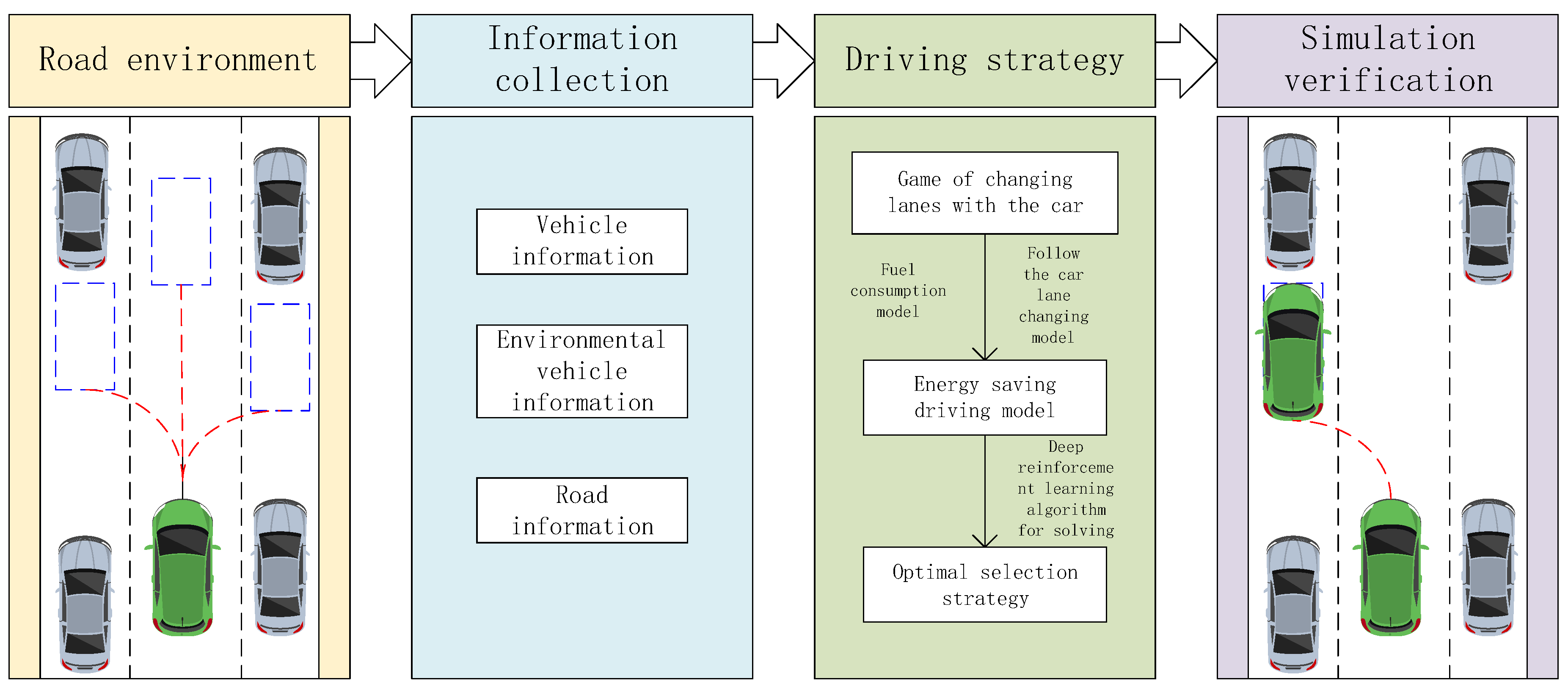
Figure 2.
Framework diagram of energy-saving driving application for connected vehicles.
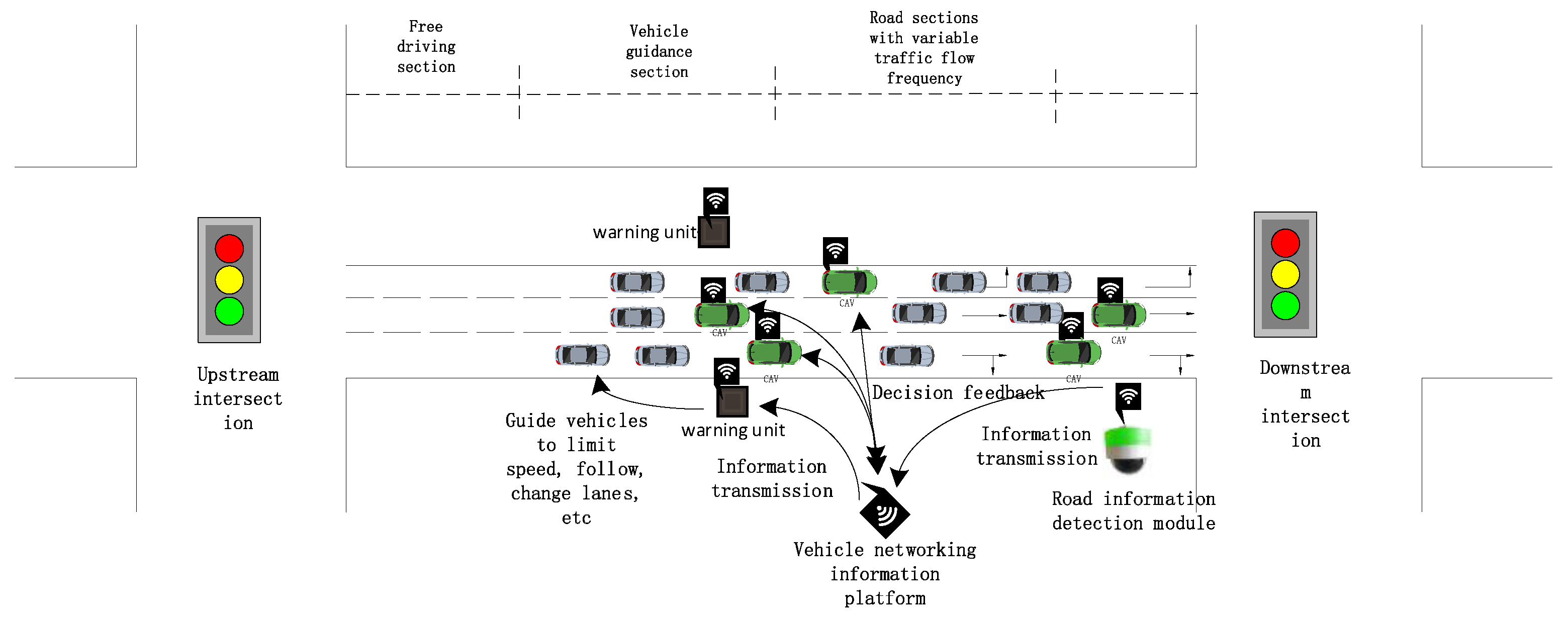
Figure 3.
Energy saving Strategy Control Flow Chart.

Figure 4.
Flow Chart of Deep Reinforcement Learning Algorithm.
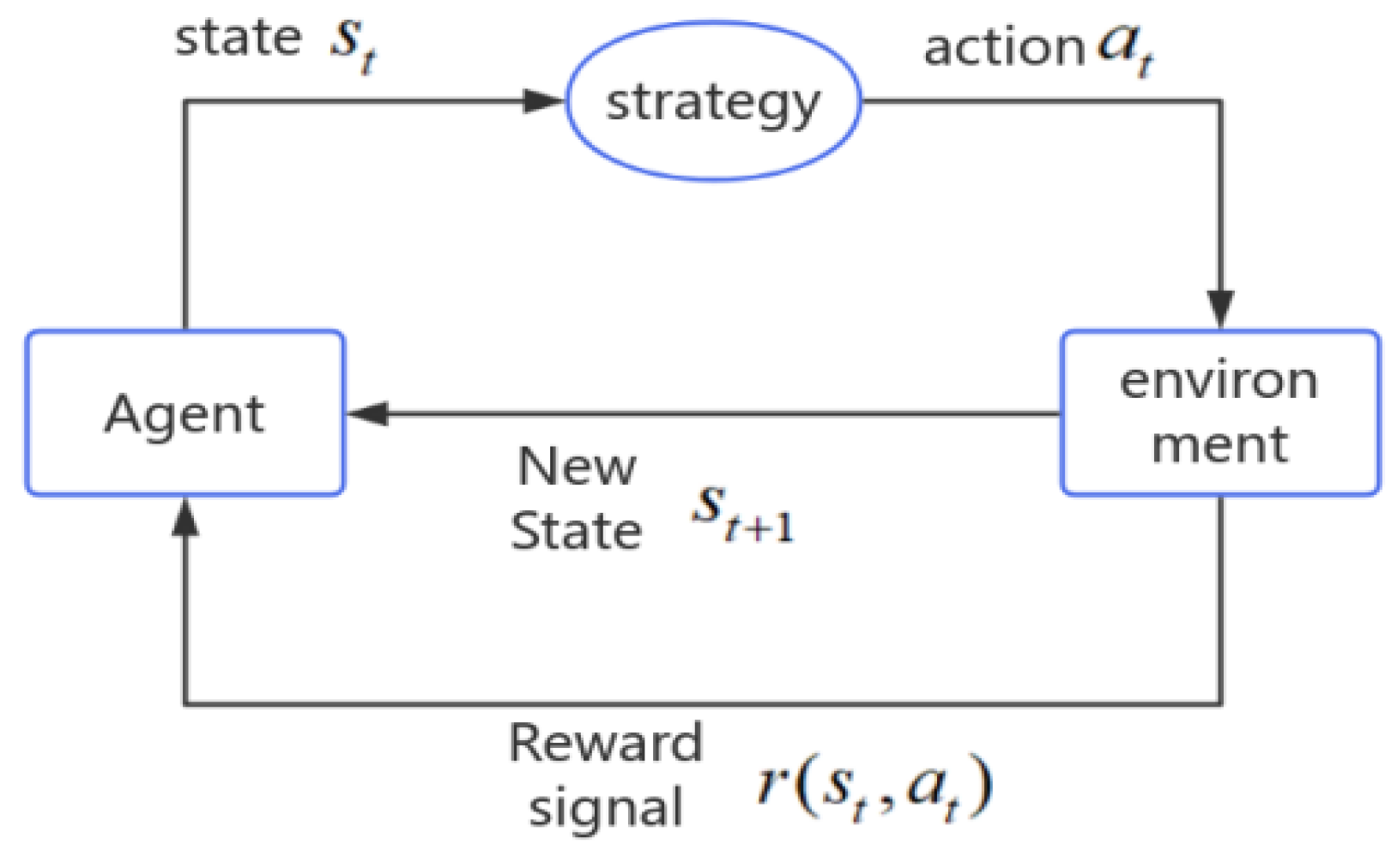
Figure 5.
D3QN algorithm model diagram.
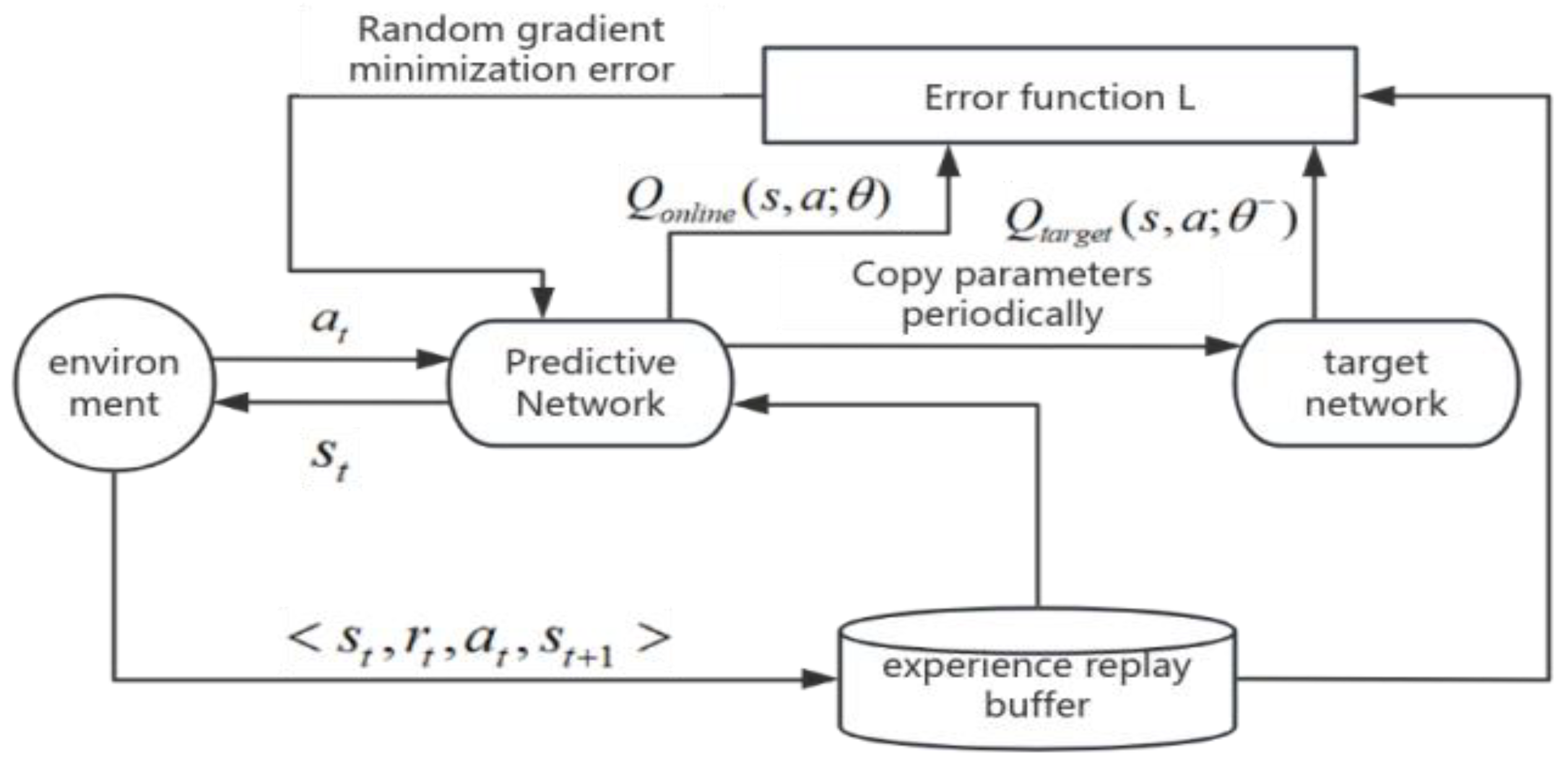
Figure 6.
D3QN Dual Branch Network Architecture Diagram.
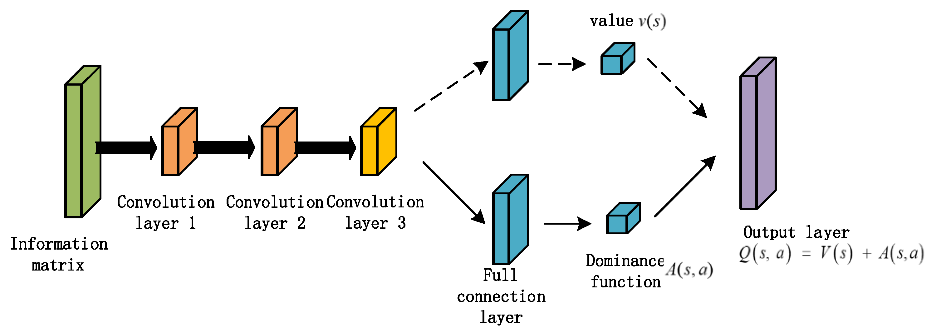
Figure 7.
Convergence Curve of D3QN Algorithm.
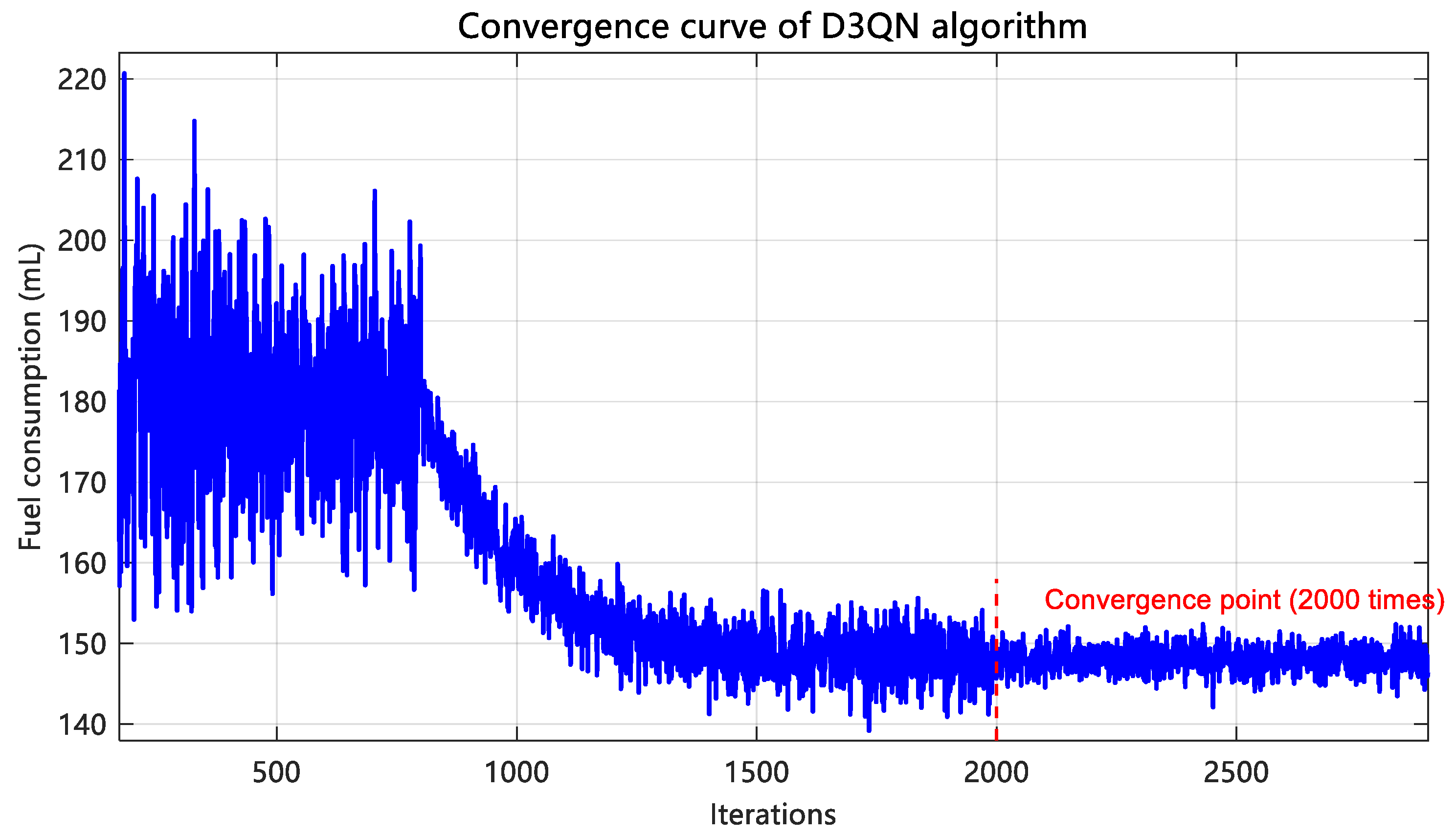
Figure 8.
Schematic diagram of the relationship between fuel consumption and traffic density under different proportions of CAV.
Figure 8.
Schematic diagram of the relationship between fuel consumption and traffic density under different proportions of CAV.
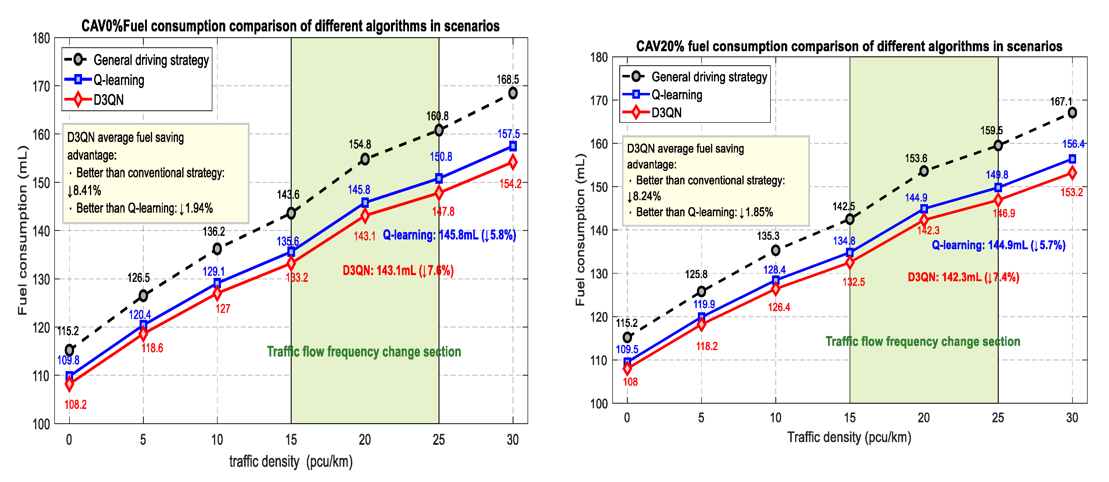
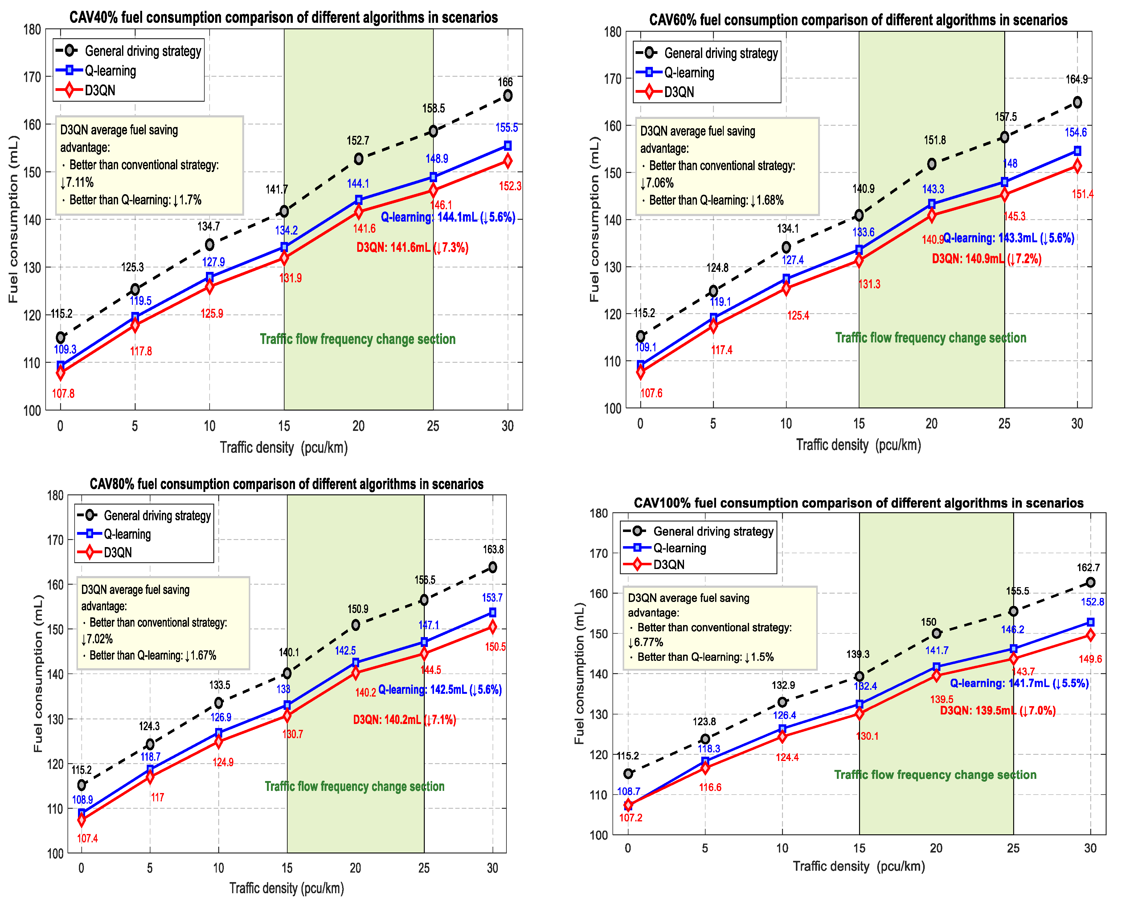
Figure 9.
Comparison of Vehicle Speed Time Series.
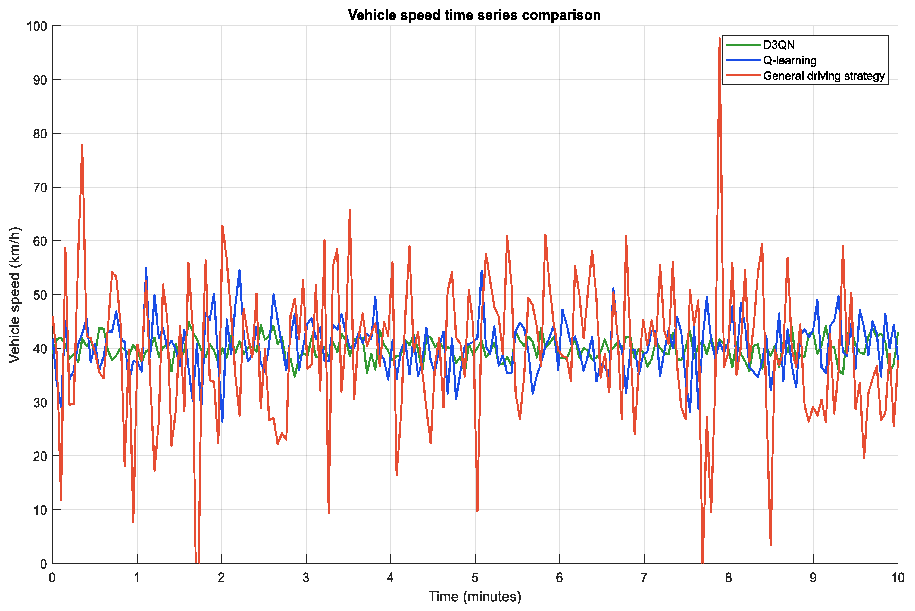
Figure 10.
Probability density distribution of vehicle speed.
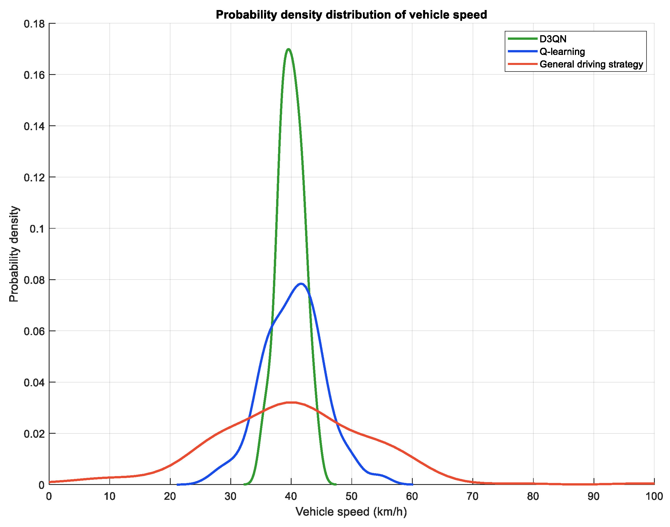

Table 1.
Simulation Parameters of Mixed Traffic Flow Model.
| Parameter | symbol | numerical value |
|---|---|---|
| road length /m | 1610 | |
| number of lanes | 3 | |
| CAV conductor/m | 5 | |
| car conductor/m | 5 | |
| Speed limit of road section(km·h-1) | 30 | |
| deceleration/(m·s-2) | 0.6 | |
| maximum deceleration/(m·s-2) | 1 | |
| starting position of road section/m | 415 | |
| end position of road section/m | 125 | |
| traffic density /(pcu·km-1) | 0~30 | |
| stochastic moderation probability | 0.2~0.5 | |
| phase interval/m | 10 |
Table 2.
D3QN Energy saving Algorithm Parameter Settings.
| Parameter | numerical value |
|---|---|
| number of training rounds | 500 |
| pre test steps | 500 |
| minimum batch size | 100 |
| discount rate | 0.90 |
| learning rate | 0.001 |
| greediness | 0.5 |
| parameter update cycle | 50steps |
| network layers | 3 |
| experience playback pool size | 500 |
| state matrix size | 1×12×1+1 |
| action space size | 3×3 |
Table 3.
Simulation Results Data Table.
| Traffic flow density |
CAV ratio/% | ||||||||||||
|---|---|---|---|---|---|---|---|---|---|---|---|---|---|
| strategy | 0 | 20 | 40 | 60 | 80 | 100 | |||||||
| fuel use | effect | fuel use | effect | fuel use | effect | fuel use | effect | fuel use | effect | fuel use | effect | ||
| 0 | Q-learning | 109.80 | 4.69% | 109.50 | 4.95% | 109.30 | 5.12% | 109.10 | 5.30% | 108.90 | 5.47% | 108.70 | 5.64% |
| D3QN | 108.20 | 6.08% | 108.00 | 6.25% | 107.80 | 6.42% | 107.60 | 6.60% | 107.40 | 6.77% | 107.20 | 6.94 | |
| 5 | Q-learning | 120.40 | 4.82% | 119.90 | 4.69% | 119.50 | 4.63% | 119.10 | 4.57% | 118.70 | 4.50 | 118.30 | 4.44 |
| D3QN | 118.60 | 6.25% | 118.20 | 6.04% | 117.80 | 5.99% | 117.40 | 5.93% | 117.00 | 5.87 | 116.60 | 5.82 | |
| 10 | Q-learning | 129.10 | 5.21% | 128.40 | 5.10% | 127.90 | 5.05% | 127.40 | 5.00% | 126.90 | 4.94 | 132.90 | 4.89 |
| D3QN | 127.00 | 6.76% | 126.40 | 6.58% | 125.90 | 6.53% | 125.40 | 6.49% | 124.90 | 6.44 | 126.40 | 6.40 | |
| 15 | Q-learning | 135.60 | 5.57% | 134.80 | 5.40% | 134.20 | 5.29% | 133.60 | 5.18% | 133.00 | 5.07 | 132.40 | 4.95 |
| D3QN | 133.20 | 7.24% | 132.50 | 7.02% | 131.90 | 6.91% | 131.30 | 6.81% | 130.70 | 6.71 | 130.10 | 6.60 | |
| 20 | Q-learning | 145.80 | 5.81% | 144.90 | 5.67% | 144.10 | 5.63% | 143.30 | 5.60% | 142.50 | 5.57 | 144.70 | 5.53 |
| D3QN | 143.10 | 7.56% | 142.30 | 7.36% | 141.60 | 7.27% | 140.90 | 7.18% | 140.20 | 7.09 | 139.50 | 7.00 | |
| 25 | Q-learning | 150.80 | 6.22% | 149.80 | 6.08% | 148.90 | 6.06% | 148.00 | 6.03% | 147.10 | 6.01 | 146.20 | 5.98 |
| D3QN | 147.80 | 8.08% | 146.90 | 7.90% | 146.10 | 7.82% | 145.30 | 7.75% | 144.50 | 7.67 | 143.70 | 7.59 | |
| 30 | Q-learning | 157.50 | 6.53% | 156.40 | 6.40% | 155.50 | 6.33% | 154.60 | 6.25% | 153.70 | 6.17 | 152.80 | 6.09 |
| D3QN | 154.20 | 8.52% | 153.20 | 8.32% | 152.30 | 8.25% | 151.40 | 8.18% | 150.50 | 8.11 | 149.60 | 8.05 | |
Disclaimer/Publisher’s Note: The statements, opinions and data contained in all publications are solely those of the individual author(s) and contributor(s) and not of MDPI and/or the editor(s). MDPI and/or the editor(s) disclaim responsibility for any injury to people or property resulting from any ideas, methods, instructions or products referred to in the content. |
© 2025 by the authors. Licensee MDPI, Basel, Switzerland. This article is an open access article distributed under the terms and conditions of the Creative Commons Attribution (CC BY) license (http://creativecommons.org/licenses/by/4.0/).
Copyright: This open access article is published under a Creative Commons CC BY 4.0 license, which permit the free download, distribution, and reuse, provided that the author and preprint are cited in any reuse.


