Fixed-Effect or Random-Effects Models? How to Choose, Perform, and Interpret Meta-Analyses in Clinical Research

Javier Arredondo Montero

doi:10.20944/preprints202509.0126.v2

Submitted:

20 October 2025

Posted:

21 October 2025

Read the latest preprint version here

Abstract

Meta-analysis has become central to evidence-based medicine, yet a persistent gap remains between statistical experts and clinicians in understanding the implications of model choice. The distinction between fixed- and random-effects is often dismissed as a technical detail, when in fact it defines the very philosophy of evidence synthesis and must be addressed conceptually, a priori, rather than dictated by heterogeneity statistics. Fixed-effect models provide a conditional inference about the average effect within the included studies, based on the assumption that differences between study estimates are due solely to sampling error. Random-effects models, by contrast, acknowledge that true effects differ across studies, populations, and settings, providing wider but more credible intervals that reflect real-world diversity. This work presents a tutorial designed to explain, in a simple and accessible manner, how to conduct an updated and robust evidence synthesis through real and simulated examples—including clinical scenarios, a worked hypothetical meta-analysis, and re-analyses of published reviews—the tutorial demonstrates how model choice can fundamentally alter conclusions. Results that appear significant under a fixed-effect model may become non-significant when using random-effects methods, due to wider confidence intervals that incorporate between-study heterogeneity. In contrast, prediction intervals reveal the range of effects likely to be observed in practice. Drawing on Cochrane guidance, the discussion highlights current standards, including REML and Paule–Mandel estimators, Hartung–Knapp–Sidik–Jonkman confidence intervals, and the routine use of prediction intervals. By combining conceptual examples with practical applications, the tutorial provides clinicians with an accessible introduction to contemporary meta-analytic methods, promoting more reliable evidence synthesis.

Keywords:

meta-analysis

;

fixed-effect model

;

random-effects model

;

heterogeneity

;

prediction intervals

;

evidence synthesis

;

Cochrane handbook

Subject:

Medicine and Pharmacology - Clinical Medicine

Introduction

Two meta-analyses, based on the very same set of studies, may yield strikingly different conclusions. For the clinician reviewing the literature, this contradiction is more than a statistical curiosity—it is a source of genuine confusion that can shape clinical decisions. Why does this happen? More often than not, the explanation lies in a modeling choice rarely discussed outside statistical circles: whether the analysis was conducted under a fixed-effect or a random-effects framework.

This choice is not a technical footnote. It determines whether the inference is conditional on the specific studies included (fixed-effect) or targets a broader superpopulation of comparable settings (random-effects).

In practical terms, it is the difference between reporting a highly precise estimate that assumes all studies are interchangeable and presenting a more cautious summary that acknowledges heterogeneity as part of clinical reality—a distinction that is foundational to clinical research [1]. Not only are such heterogeneity statistics misused to dictate model choice, but doing so confuses cause and effect: model philosophy should be set conceptually a priori, not driven by an I² value.

For clinicians, understanding this distinction is essential. This distinction reframes meta-analysis: it is not only a tool for producing a single summary estimate, but also for interpreting the variability of evidence. This article offers a foundational explanation of fixed versus random effects. This work aims not only to clarify statistical modeling but also to demonstrate why model choice carries direct consequences for how evidence is translated into practice.

The Foundational Question: One True Effect?

At its heart, the choice of model boils down to this: do we believe that every study is measuring the same single effect, or do we accept that true effects differ from one study to another? [2]

The fixed-effect model assumes the former. It treats each study as a repeated measurement of the same underlying truth, with differences explained solely by chance. In this view, there is one “true effect,” and the task of meta-analysis is to identify it with the greatest possible precision.

The random-effects model assumes the latter. It acknowledges that effects may legitimately differ across settings, populations, and methods. Rather than assuming one universal truth, it estimates the average of a distribution of true effects and incorporates that variability into the pooled estimate [3].

A clinical metaphor illustrates the distinction. Consider multiple experiments designed to measure the acceleration due to gravity (g):

In this setting, a fixed-effect model would be appropriate: it assumes there is a single universal true value for g (approximately 9.81 m/s²), and that any variation between experimental estimates arises solely from measurement error (i.e., sampling error). The goal of the meta-analysis would be to obtain the most precise possible estimate of this single underlying constant.
Now compare this with a clinical example: estimating the average systolic blood pressure (SBP) of adults in different cities. Here, a random-effects model is more appropriate. We do not assume that all cities share the same true SBP. Instead, we assume that each city has its own true mean SBP, and that these values are drawn from a broader distribution shaped by demographic, lifestyle, and environmental factors. The aim of a random-effects meta-analysis, therefore, is not to estimate a single fixed constant, but to estimate the mean of this distribution and quantify how much the true effects vary across settings (the between-study variance, τ²).

The choice between these models is not a mere technical detail; it reflects a fundamental, and still active, debate about the primary goal of meta-analysis. A fixed-effect model provides a precise answer to the question: ‘What is the best estimate of the average treatment effect in the specific set of studies included in this review?’. This is known as a conditional inference (that is, the conclusion applies only to the particular studies included in the meta-analysis, and does not generalize beyond them). In contrast, a random-effects model addresses a broader question: ‘What is the best estimate of the average treatment effect in the wider universe of potential studies from which our included studies are considered a sample?’. This is an unconditional inference. Neither question is inherently superior; the appropriate model depends on the research objective and the plausibility of its underlying assumptions. Choosing between them is not just a statistical decision—it determines whether we present evidence as a single number or as a distribution that mirrors clinical practice.

This distinction is inferential rather than rhetorical: fixed-effect estimation targets a conditional mean restricted to the included studies, whereas random-effects targets an unconditional mean intended to generalize to comparable future settings.

Table 1 provides additional clinical examples that illustrate how fixed- and random-effects models embody fundamentally different assumptions, leading to distinct interpretations of the same evidence.

Fixed-Effect: Clarity with a Cost

The appeal of the fixed-effect model lies in its apparent simplicity. By treating every study as a replicate of the same underlying truth, it produces a single pooled estimate with narrow confidence intervals. This precision can be appealing, as it seems to offer a definitive answer.

Yet this clarity comes at a cost. If true effects genuinely differ across settings, the fixed-effect model, by design, does not model this variability. The result is a precise estimate conditional on the included studies, which may have limited generalizability if true heterogeneity exists.

Under a fixed-effect view, the underlying effect is treated as a constant—analogous to assuming that gravitational acceleration is identical in every measurement context. In meta-analyses of non-randomized studies, where study-level confounding is a significant concern, the fixed-effect model may therefore be preferred precisely because its conditional inference is robust to this type of confounding.

The primary strength of the fixed-effect model lies in its robustness to study-level confounding: by conditioning inference on the included studies, it removes all sources of between-study variability from the pooled estimate. Any stable study-level characteristic—such as differences in patient populations, study quality, or local protocols—is, by construction, fully controlled for, whether measured or unmeasured. However, this robustness is extremely narrow in scope and is purchased at the complete expense of generalizability. The resulting estimate is valid only for this specific set of studies and provides no statistical basis for extending the inference to future settings or populations. Crucially, this does not make the fixed-effect model a “safer” or more “valid” option when confounding is present. It simply changes the target of inference from a clinically useful question (“what can we expect in comparable settings?”) to a much narrower one (“what was the average effect exclusively in these exact studies?”). For this reason, the presence of confounding cannot serve as a post hoc justification for selecting a fixed-effect model when the inferential goal is to inform clinical practice or policy; model choice must remain an a priori decision tied to the intended scope of inference, not a reactive methodological tactic.

The cost of this robust confounding control is a limitation in generalizability. The inference from a fixed-effect model is conditional on the specific studies included and cannot be generalized statistically to a wider population of studies. Any extension beyond the included sample relies on external, non-statistical justification.

Random-Effects: Embracing Variability

In contrast, the random-effects model begins from a different premise: that variation across studies is not merely noise, but often reflects genuine differences between them. These differences may arise from multiple sources—such as populations, clinical settings, or how an intervention is implemented. Instead of forcing all studies into a single truth, the random-effects model estimates the mean of a distribution of true effects and widens the confidence interval to reflect that diversity.

Under a random-effects framework, study estimates are treated as samples from a distribution of true effects rather than measurements of a single fixed quantity. This reflects the goal of unconditional inference — generalizing to a wider superpopulation of settings beyond those observed.

Clinically, this perspective often aligns with the expectation that effects may vary across settings, populations, and implementation contexts. As shown in Table 1, the benefit of screening colonoscopy may be greater in well-resourced, high-coverage programs and smaller in under-resourced settings. The blood-pressure response to ACE inhibitors differs across patient groups, shaped by comorbidity, adherence, baseline risk, and even race. Random-effects models explicitly incorporate such heterogeneity into the summary estimate.

While the random-effects model offers greater generalizability, it relies on the strong assumption that the true study effects (the random effects) are uncorrelated with study-level covariates. If unmeasured confounders exist that are associated with the treatment effect, this assumption is violated, and the pooled estimate may be biased. Therefore, while the model embraces variability, it is more susceptible to bias from study-level confounding than its fixed-effect counterpart.

The price to pay is less apparent precision. Confidence intervals under random-effects are usually wider. Put simply, a confidence interval is the range of values within which the true effect is most likely to lie. A narrow interval may look more reassuring, but if it ignores genuine variation, it can be misleading. Wider intervals under random-effects are not a weakness—they quantify an additional, modeled source of uncertainty (the between-study variance).

In practice, random-effects analysis acknowledges what every clinician already knows: patients, hospitals, and health systems are not identical. By incorporating between-study variance, random-effects inference reflects the expected dispersion of effects when applied in new but comparable settings.

Heterogeneity as the Compass for Model Choice

What Heterogeneity Means

Heterogeneity means that the results of studies are not identical [4,5,6,7,8,9]. Sometimes this variation is small and trivial; other times it is substantial and clinically meaningful. In meta-analysis, the key question is not whether differences exist—they almost always do—but whether these differences should be interpreted as random noise around a single true effect or as evidence that the true effects genuinely differ across settings.

Clinical vs. Statistical Heterogeneity

Two forms of heterogeneity should be distinguished:

Clinical heterogeneity: real-world variability in who was studied, what was done, or where it was done. These differences are not “errors” but reflections of normal clinical diversity (e.g., different patient profiles, dosages, techniques, or healthcare settings).
Statistical heterogeneity: heterogeneity “put into numbers.” It describes how much the study estimates differ after accounting for sampling error (i.e., the random imprecision that arises simply because each study observes only a finite sample of patients). Indices like Q, I², and τ² express this variance quantitatively.

Quantifying and Interpreting Heterogeneity

There are several common tools, each with a distinct role:

Cochran’s Q: a χ² (chi-squared) test of the null hypothesis that all studies estimate the same true effect [4]. It checks whether observed dispersion exceeds what would be expected by chance. Q has low power with few studies and excessive sensitivity with many; therefore, a non-significant Q should never be interpreted as evidence of homogeneity.
I²: the percentage of total variation explained by real heterogeneity rather than chance [2,5,6]. Values of 25%, 50%, and 75% are often quoted as low, moderate, and high, but these thresholds are arbitrary and context-dependent. I² is only an estimate and can be unstable with few studies, and because it depends on study precision, large datasets can yield high I² even when absolute differences are clinically trivial. For this reason, I² should be interpreted descriptively and should not dictate model choice.
τ² (between-study variance): an absolute measure of how much true effects differ across studies, expressed on the same scale as the effect size [2,7,8]. A τ² close to zero indicates minimal dispersion of true effects; larger τ² values indicate meaningful underlying variability. τ² drives the weights in random-effects models and determines the width of confidence and prediction intervals. However, it quantifies heterogeneity — it does not explain its sources. Explaining heterogeneity requires further investigation (e.g., subgroup analysis or meta-regression).

Choosing an Estimator for τ²

The choice of how to estimate τ² can meaningfully influence the results of a random-effects meta-analysis. Several estimators exist:

DerSimonian–Laird (DL): the traditional, non-iterative estimator derived from Cochran’s Q statistic [10]. Although historically common and still the default in older software, numerous simulation studies have shown that DL is often negatively biased, systematically underestimating the true between-study variance τ², especially when the number of studies is small or when events are rare. This underestimation leads to overly narrow confidence intervals and an inflated Type I error rate.
Restricted Maximum Likelihood (REML): an iterative estimator that is generally more robust. Simulation studies consistently demonstrate that REML yields a less biased estimate of τ² across a wide range of realistic meta-analytic scenarios compared with DL. For this reason, it is now recommended as the default option in many methodological guidelines, including the Cochrane Handbook.
Paule–Mandel (PM): another robust iterative estimator that frequently performs similarly to REML. PM is also considered a superior alternative to DL and is likewise endorsed by Cochrane as an appropriate default when heterogeneity is expected.

Calculating Confidence Intervals (“the CI”)

Once the average effect is estimated, we need to decide how wide the confidence interval should be.

Wald CI: the traditional, straightforward approach; it often produces intervals that look reassuringly precise but can be too narrow, especially when there are few studies or some heterogeneity [2].
Hartung–Knapp–Sidik–Jonkman (HKSJ): a modern method that produces wider and generally more reliable intervals. It is now considered the standard when heterogeneity is present. With very few studies, it can sometimes yield excessively wide (over-conservative) intervals; however, it remains the better option overall, as cautious inference is safer than overconfident conclusions [11,12].
Modified or truncated HKSJ (mHK): a refinement of the HKSJ method, designed to prevent confidence intervals from becoming excessively wide in rare situations—typically when the number of studies is very small, a common scenario in clinical research, or when the between-study variance is close to zero [13].

A key limitation of all random-effects models is the difficulty of accurately estimating the between-study variance, τ², when the number of included studies is small. With fewer than about ten studies, estimates of τ² are typically unstable, highly imprecise, and often biased—sometimes severely so. Some methodologists recommend at least 20–30 studies for a reliably estimated τ², although such sample sizes are rarely available in clinical research. This instability is precisely why modern inference methods—most notably the HKSJ adjustment—are recommended: they explicitly account for the uncertainty in τ², producing wider but more appropriate confidence intervals when evidence is sparse.

Random-effects models all share the same philosophy—accepting variability—but they differ in how cautious they are. DL + Wald often looks neat and “precise” but can be misleading. REML or Paule–Mandel combined with HKSJ intervals are increasingly seen as the safer choices when evidence is sparse or heterogeneous [2].

Model Choice Should Come First (and I² Should Not Be Used to Make This Choice)

Crucially, the choice between a fixed- or random-effects framework is conceptual and should be made before examining heterogeneity statistics [2]. The key question is whether we believe in a single underlying effect (fixed-effect) or a distribution of effects (random-effects). Q, I², and τ² describe heterogeneity — they do not determine the philosophical model. Selecting a model reactively based on I² thresholds is methodologically unsound.

Putting It Together

In practice, heterogeneity is expected in nearly all clinical meta-analyses. When studies are highly consistent, fixed- and random-effects estimates converge. When they diverge, random-effects models more accurately capture reality, whereas fixed-effect approaches may suppress meaningful variability. Heterogeneity is therefore not a flaw to be corrected, but a guide that helps interpret whether — and for whom — a result is likely to hold.

Prediction Intervals: Looking Beyond Confidence Intervals

Confidence intervals describe the precision of the average effect. Prediction intervals (PIs), by contrast, indicate the range of effects that might plausibly be observed in a new but comparable setting [3,14,15]. This distinction matters clinically: many meta-analyses appear “statistically significant,” yet their PIs include the null — a red flag indicating fragile or context-dependent effects. Large-scale re-analyses show this occurs in nearly 75% of cases [16]. By reporting PIs alongside CIs, meta-analysts provide a more realistic expectation of real-world performance in future populations. Prediction intervals can only be calculated within a random-effects framework when the estimated between-study variance (τ²) is greater than zero. When τ² is estimated as zero, the random-effects model collapses to the fixed-effect model, and the PI becomes identical to the CI.

So, Which Model Should I Choose?

Key Principles for Model Choice

Once the conceptual distinction has been made—that fixed-effect yields a conditional inference and random-effects an unconditional one—the practical question becomes how to choose a model in applied work. The choice should follow from the inferential target, not from heterogeneity statistics.For this reason, model choice should be made conceptually, before looking at any statistics. Numbers like Q, I², or τ² are useful for describing how much studies vary, but they do not determine the philosophy of the model. The starting point must always be the question: do we believe in one effect, or in many? It is the same distinction as asking whether we are measuring a single physical constant (like gravity) or the average of a variable measure (like systolic blood pressure across different hospitals).

Table 2 summarizes the key criteria that distinguish fixed-effect from random-effects models and guides the use of each when they may be appropriate in clinical meta-analysis.

What Cochrane Recommends

The Cochrane Handbook is explicit on this issue [2]. Random-effects models are generally the safer choice whenever clinical diversity is present—meaning, in most clinical questions. Fixed-effect can be defensible only when studies are virtually identical in design, participants, and context, a situation that is rare outside very narrow questions.

Cochrane also warns against a common mistake: switching between models based on whether I² is “high” or “low.” Heterogeneity statistics describe variability, but they should not dictate the model. Instead, the model should be chosen a priori, guided by the plausibility of one universal effect versus a distribution of effects. Increasingly, Cochrane reviews present both random-effects as the main analysis and fixed-effects as a sensitivity check.

Table 3 reports the explicit recommendations of the Cochrane Handbook on model choice and inference, together with their practical implications for clinical meta-analysis.

Practical Guidance for Clinicians

For clinicians interpreting meta-analyses, several practical lessons can be drawn. In most applied settings, random-effects is conceptually aligned to generalize beyond the included studies. Fixed-effect has a role, but mainly as a sensitivity analysis (for example, if the FE and RE estimates are similar, it suggests the finding is robust to model choice; if they diverge, it signals that heterogeneity meaningfully affects inference) or in narrowly defined questions where studies are genuinely homogeneous.

Statistical significance under fixed-effect should not be mistaken for robustness. If a result disappears when random effects are applied, hat indicates that variability matters and the evidence is heterogeneous. Finally, always look at the forest plot before the summary number. If studies point in different directions, an apparently precise fixed-effect estimate has limited generalizability. Likewise, a single pooled estimate under a fixed-effect framework may obscure whether the effect remains stable across settings.

Making It Visual: Fixed vs Random at a Glance

The contrast between fixed- and random-effects models is not only conceptual but also readily visible. ure 1 presents, for illustrative purposes, a simulated meta-analysis of six randomized trials evaluating a hypothetical new antithrombotic agent for the prevention of postoperative thrombosis. Each trial compared the novel drug with conventional prophylaxis, reporting the number of thrombotic events in each group. While all studies suggested fewer events in the treatment arm, the magnitude of benefit varied substantially across trials.

Figure 1. Simulated meta-analysis of six randomized trials of a new antithrombotic agent for postoperative thromboprophylaxis. Each study reports the number of thrombotic events in the treatment (novel agent) and control (conventional prophylaxis) groups. The top panel displays the fixed-effect Mantel–Haenszel model (RR 0.73, 95% CI 0.62–0.87, p < 0.01). The middle panel shows the random-effects model using the REML estimator of τ² (RR 0.76, 95% CI 0.58–0.99, p = 0.04), with between-study variance τ² = 0.05, heterogeneity I² = 50.8%, and Q = 10.96 (p = 0.05); Wald confidence intervals are presented. The bottom panel illustrates the random-effects model using REML with Hartung–Knapp adjustment (RR 0.76, 95% CI 0.55–1.05, p = 0.08), where τ² = 0.05, I² = 50.8%, and Q = 10.96 (p = 0.05); confidence intervals are based on the Hartung–Knapp method. For the random-effects models, the 95% prediction interval (0.36–1.57) indicates that the effect in a future study could plausibly range from substantial benefit to no benefit—or even harm, underscoring the importance of model choice in clinical interpretation. All analyses were performed using Stata version 19.0 (StataCorp LLC, College Station, TX, USA), employing the meta package. A small note for readers: if the analyses are replicated under a Mantel–Haenszel fixed-effect model or using the DerSimonian–Laird method, the heterogeneity summaries will be slightly different from the REML-based figures reported here—specifically, Q = 11.06 on 5 degrees of freedom (p = 0.05) and I² = 54.8%. This occurs because Q and its derivative I² are formally defined within a fixed-effect framework, where study weights depend only on within-study variance. When software such as Stata recalculates these indices using random-effects weights (as in REML), the values shift modestly. Conceptually, the “canonical” values are those from the fixed-effect calculation (54.8% here); DL is consistent with this convention because it computes Q using fixed-effect inverse-variance weights.

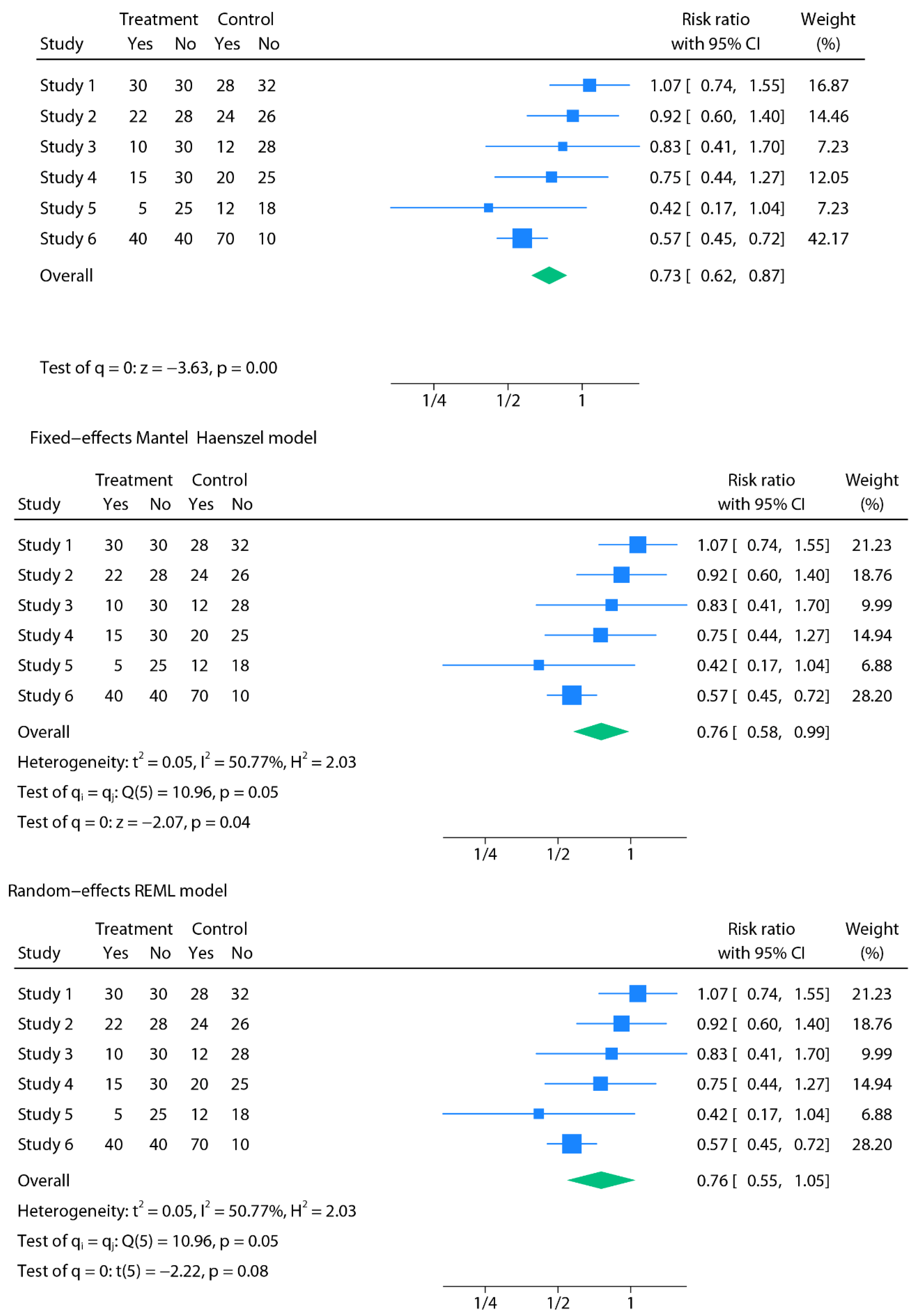
Under a fixed-effect Mantel–Haenszel model (a fixed-effect pooling method), pooling the six studies yielded a statistically significant reduction in thrombotic events with narrow confidence intervals (RR 0.73, 95% CI 0.62–0.87; p<0.01). At face value, this implies that the new antithrombotic reduces postoperative thrombosis by roughly 27% in every surgical context. However, when a random-effects model with REML estimation was applied, the pooled effect remained directionally similar but the confidence interval widened (RR 0.76, 95% CI 0.58–0.99; p = 0.04). Incorporating the Hartung–Knapp adjustment further broadened the interval, rendering the result statistically non-significant (RR 0.76, 95% CI 0.55–1.05; p = 0.08).

Most importantly, the prediction interval revealed the fragility of the evidence: in a future trial, the true effect could plausibly range from a 64% risk reduction to a 57% risk increase (95% PI 0.36–1.57). In other words, while some surgical populations might experience substantial benefit, others could see little to no advantage—or even possible harm. With moderate heterogeneity (I² = 50.77%, Q = 10.96, p = 0.05, τ² = 0.05), this example underscores how fixed-effect analysis may create the illusion of a universal benefit, whereas random-effects modelling more faithfully represents the uncertainty and variability encountered in clinical practice.

The heterogeneity observed in this example could plausibly arise from multiple sources: Do all patients across trials share the same baseline thrombotic risk, or were study populations selected differently? Were thrombotic events documented consistently across centers, or did outcome assessment vary? Were prophylaxis protocols strictly adhered to in all trials, or was implementation uneven? These questions illustrate that heterogeneity is not a nuisance but often reflects genuine clinical and methodological differences that need to be acknowledged rather than averaged away.

How to Report a Meta-Analysis

Methods

Transparency in methods is essential. A well-reported meta-analysis should clearly state which statistical model was used (fixed- or random-effects, with the specific estimator such as DerSimonian–Laird, Paule–Mandel, or REML), the software and commands employed, and the planned strategies to explore heterogeneity. This includes pre-specified subgroup analyses (e.g., by population, setting, or intervention dose), sensitivity analyses (e.g., excluding high-risk-of-bias studies), and, when appropriate, meta-regression. Any continuity corrections (adjustments for studies with zero events in one arm) should be explicitly described. Common methods include adding a fixed value (e.g., 0.5) to all cells, which can introduce bias, or the treatment-arm continuity correction (TACC), which scales the adjustment to the size of each study arm and is often preferred for ratio measures. As different corrections can yield different results, the choice should be pre-specified. By laying out these choices in advance, the analysis avoids the perception of selective reporting and allows full reproducibility. Continuing with the SBP metaphor, report not only the mean SBP across cities (e.g., 122 mmHg), but also the spread of the true city-level means (i.e., τ² and the PI), as both are important for interpretation. Equally important, meta-analyses should adhere rigorously to established methodological standards. The Cochrane Handbook for Systematic Reviews of Interventions provides detailed guidance on appropriate model selection, heterogeneity assessment, and sensitivity analyses [2]. At the same time, the PRISMA 2020 statement ensures transparent and complete reporting of methods and results [17]. Following these frameworks not only strengthens methodological rigor but also facilitates critical appraisal, reproducibility, and trust in the evidence synthesized.

Results

In the results section, findings should be presented with forest plots that are legible and fully annotated, showing study-level estimates, pooled effects, and heterogeneity measures (Q, I², τ²). Both confidence intervals (CI) and, when possible, prediction intervals (PI) should be reported to convey not only the precision of the mean effect but also the likely range of effects in future settings. The type of model and interval calculation method (e.g., Wald vs. Hartung–Knapp–Sidik–Jonkman) must be specified, since some software packages (such as CMA) provide only default or limited options. If continuity corrections were applied, these must also be reported, with justification for the chosen method. Above all, the principle of maximum transparency is paramount: every analytical choice should be transparent to the reader, ensuring that conclusions are seen as robust and reproducible.

Table 4 summarizes the essential elements that should be transparently reported in the methods and results of a meta-analysis, including model choice, heterogeneity measures, confidence and prediction intervals, and sensitivity analyses.

A Practical Workflow for Performing a Meta-Analysis

To address the gap between conceptual explanation and applied implementation highlighted by Reviewer 3, this section provides a concise step-by-step workflow outlining how a meta-analysis is actually fitted in practice—from data extraction to final inference. The purpose is not to train readers in software syntax, but to make explicit what each modelling step consists of, so that the technical decisions later reported in the Methods and Results become transparent and interpretable.

Step 1 — Define and Extract the Effect Size

The analyst must first determine which effect measure is appropriate (e.g., log risk ratio, log odds ratio, mean difference, or standardized mean difference) and extract both the estimate and its corresponding sampling variance for each included study. These two quantities—effect size and variance—are the essential inputs required by all meta-analytic models.

Step 2 — Specify the Modelling Framework

Before looking at heterogeneity statistics, a conceptual decision is made between a fixed-effect model (assuming a single underlying true effect) or a random-effects model (assuming a distribution of true effects across studies). This is a philosophical choice about the target of inference, not a reactive decision based on I² or Q.

Step 3 — Choose How Between-Study Heterogeneity Is Estimated

Under random-effects, a τ² estimator must be selected. Contemporary methodological guidance recommends REML or Paule–Mandel because they yield more stable and less biased estimates than the traditional DerSimonian–Laird estimator, particularly when few studies are available or effects are heterogeneous.

Step 4 — Choose How Uncertainty Is Quantified

Once the pooled estimate is obtained, the analyst must select a confidence interval method. Wald intervals often appear narrow but can be misleading. Modern guidance recommends Hartung–Knapp–Sidik–Jonkman, which better reflects real uncertainty, especially with small evidence bases.

Step 5 — Interpret Heterogeneity

Only after the model is fitted are heterogeneity statistics (τ², I², Q) interpreted. These numbers summarise how much true variability exists between studies—but they do not determine the model itself. Their role is descriptive and interpretive, not decisive.

Step 6 — Report Generalizability via Prediction Intervals

A prediction interval extends inference from “what is the average effect?” to “what range of effects might realistically appear in a future setting?”. This clarifies whether results are broadly applicable or highly context-dependent.

Step 7 — Sensitivity and Transparency

Finally, the analysis should document:

which modelling framework was used (fixed vs random-effects),
which τ² estimator was applied (e.g., REML or Paule–Mandel),
which CI method was used (e.g., Hartung–Knapp),
and whether continuity corrections or other analytical adjustments were required.

These steps together define what it means to “fit” a meta-analysis in practice. They make the workflow explicit and reproducible, bridging the gap between methodological principles and concrete analytical execution.

Real-World Case Studies: How Fixed vs Random-Effects Alter Conclusions

Applied Case Study 1: Urination Stimulation Techniques in Infants

Clean urine collection in non-toilet-trained infants is clinically challenging: invasive methods, such as suprapubic aspiration, are painful, while non-invasive alternatives, like urine bags, are prone to contamination. Recently developed stimulation techniques (e.g., Herreros’ tapping/massage and the Quick-Wee cold gauze method) aim to facilitate voiding in infants under one year. The available trials, however, differ in infant age, maneuver applied, clinical setting, and outcome definitions, introducing substantial heterogeneity. In this context, the expectation of heterogeneity is clinically grounded: the included trials differed in infant age distribution, type and duration of the stimulation maneuver, ambient temperature during collection, and operational definitions of “successful voiding,” all of which plausibly affect the magnitude and timing of urine response.

A published meta-analysis applied a fixed-effect Mantel–Haenszel model, pooling three small, randomized trials and reporting a precise and statistically significant effect (OR 3.88, 95% CI 2.28–6.60; p < 0.01; I² = 72%) [18]. This approach assumes identical efficacy across studies, an assumption that may not hold given the clinical diversity. When the data were re-analysed using a random-effects model with REML estimation, the effect remained directionally similar but with wider confidence intervals (OR 3.44, 95% CI 1.20–9.88; p = 0.02). With the Hartung–Knapp–Sidik–Jonkman (HKSJ) adjustment, recommended for small and heterogeneous datasets, the interval widened further and statistical significance was lost (OR 3.44, 95% CI 0.34–34.91; p = 0.15) [19]. This scenario (k=3) highlights the critical challenge of estimating τ² with very few studies. Wald-type intervals (p = 0.02) rely on the unstable point estimate of τ² and are likely anti-conservative (too narrow). The Hartung–Knapp–Sidik–Jonkman (HKSJ) adjustment is specifically designed for this scenario: rather than trusting the uncertain τ² estimate, it incorporates its instability into the final confidence interval, which widens appropriately and yields a non-significant result (p=0.15). This example demonstrates that when evidence is sparse, random-effects inference remains valid, but must explicitly propagate τ² uncertainty—precisely what HKSJ achieves.

Applied Case Study 2: Musculoskeletal Outcomes After Esophageal Atresia Repair

Children with esophageal atresia (EA) require surgical repair, most commonly through conventional open thoracotomy repair (COR) or thoracoscopic repair (TR). Long-term musculoskeletal sequelae—such as scoliosis, rib fusion, and scapular winging—are recognized complications, particularly after open procedures involving rib spreading. A recent meta-analysis compared TR with thoracotomy; however, the included studies varied in follow-up duration, diagnostic methods (clinical assessment versus imaging), and surgeon expertise. These differences introduce clinical heterogeneity, making the assumption of a single common effect less plausible.

Here, heterogeneity is likewise mechanistically plausible: the trials differed in surgeon experience, thoracoscopic learning-curve stage, postoperative follow-up duration, and the diagnostic modality used to detect musculoskeletal sequelae (clinical vs radiographic), each of which could legitimately alter the observed effect size.

In this setting, the analysis employed a fixed-effect Mantel–Haenszel model, reporting statistically significant and precise reductions in musculoskeletal complications with TR (e.g., scoliosis: RR 0.35, 95% CI 0.14–0.84; p = 0.02) [20]. With only four small retrospective studies and moderate inconsistency (I² = 38%), a random-effects model using REML estimation yielded wider intervals and reduced certainty (RR 0.35, 95% CI 0.09–1.36; p = 0.13). When the Hartung–Knapp–Sidik–Jonkman (HKSJ) adjustment was applied, the confidence interval broadened further, and statistical significance was lost (RR 0.35, 95% CI 0.05–2.36; p = 0.18) [21]. As in the previous case, the small number of studies (k = 4) provides insufficient information to estimate τ² with precision. The fixed-effect estimate is conditionally valid for the included studies, but its apparent precision does not generalize. The HKSJ adjustment appropriately reflects the uncertainty in τ², yielding a wider and more cautious interval.

This case illustrates how fixed-effect modelling can produce narrow intervals that may overstate certainty. In contrast, random-effects approaches, particularly REML with HKSJ adjustment, provide a more cautious and clinically appropriate interpretation.

Applied Case Study 3: Re-Analysis of Psychological Bulletin Meta-Analyses

While some foundational re-analyses were published more than a decade ago, they remain instructive because they illustrate how model choice systematically alters inference when diversity across studies is genuine rather than random noise. Schmidt et al. revisited 68 meta-analyses published in Psychological Bulletin, many of which had relied on fixed-effect models as their primary approach. They aimed to test whether this choice was justified, given that most sets of studies in psychology—and, by extension, in medicine—are drawn from diverse populations, designs, and settings, where assuming a single common effect is unrealistic.

When they re-analysed the same datasets using random-effects procedures, the results changed substantially. Confidence intervals that had looked narrow and precise under fixed-effect became much wider, and in many cases, the apparent statistical significance disappeared. On average, the “95% CIs” reported with fixed-effect overstated precision by about half, giving an impression of robustness that the data did not actually support.

The key conclusion was that only in a small minority of cases (~3%) could a fixed-effect model reasonably be defended. In the overwhelming majority, random-effects models better captured the genuine variability between studies [22]. This large-scale re-analysis showed convincingly that reliance on fixed-effect can create an illusion of certainty and systematically exaggerate confidence in meta-analytic findings.

Applied Case Study 4: the Rosiglitazone Link with Myocardial Infarction and Cardiac Death

Shuster et al. revisited the influential meta-analysis by Nissen and Wolski on rosiglitazone and cardiovascular risk [23]. The original authors had chosen a fixed-effect approach, arguing that homogeneity tests did not reject the null. However, this decision was problematic: with rare adverse events and many trials, such tests have very low power. Moreover, the studies pooled differed substantially in dose, comparators, follow-up, and populations—conditions that make the assumption of a single common effect implausible. When Shuster and colleagues re-analysed the 48 eligible trials using random-effects methods specifically adapted for rare events, the findings shifted. For myocardial infarction, the fixed-effect model suggested statistical significance (RR 1.43, 95% CI 1.03–1.98, p = 0.03), whereas the random-effects estimate was non-significant (RR 1.51, 95% CI 0.91–2.48, p = 0.11). Conversely, for cardiac death, the fixed-effect result was null (RR 1.64, 95% CI 0.98–2.74, p = 0.06), but the random-effects analysis indicated a clear increase in risk (RR 2.37, 95% CI 1.38–4.07, p = 0.0017). The key message was that reliance on fixed-effect models, especially in the rare-event setting, can both mask and exaggerate signals depending on how large studies dominate the weights. By contrast, random-effects better accounted for the true diversity of trial scenarios. This re-analysis underscored that method choice was not a technical detail: for rosiglitazone, it meant the difference between concluding “no risk” and identifying a serious safety concern.

Applied Case Study 5: The Role of Magnesium in Acute Myocardial Infarction

A meta-analysis of 12 randomized trials assessed intravenous magnesium for acute myocardial infarction. Under a fixed-effect model, the pooled odds ratio was null (OR 1.02, 95% CI 0.96–1.08), but heterogeneity was extreme (p < 0.0001), driven largely by a single large trial where magnesium was administered late, often after fibrinolysis. Applying a random-effects model changed the conclusion: the pooled odds ratio indicated significant benefit (OR 0.61, 95% CI 0.43–0.87; p = 0.006) [24]. Experimental data support that magnesium’s cardioprotective effect depends on timely administration—before or at reperfusion, not after. Here, heterogeneity reflected a true effect modifier (timing), not random noise. This case illustrates that fixed-effect pooling can obscure clinically meaningful patterns, whereas random-effects better accommodate mechanistic plausibility and context. Importantly, the fixed-effect estimate was conditionally correct for the specific collection of studies analysed; what it failed to provide was a generalisable estimate applicable beyond that narrow sample—an inferential gap that random-effects is specifically designed to address.

Table 5 summarizes how conclusions shifted in the five real-world case studies when analyses were re-examined under random-effects models, highlighting how methodological choice can transform the apparent certainty and even the direction of evidence.

Taken together, these five case studies illustrate a single unifying lesson: the difference between fixed- and random-effects results is not stylistic or optional, but flows directly from how each model allocates weight to the individual studies. Fixed-effect models allow a single large or highly precise study to dominate the overall estimate, which can obscure meaningful variability. Random-effects models distribute influence more evenly across studies, especially when heterogeneity is present, producing a synthesis that is more stable, balanced, and credible in real clinical settings.

A Final Nuance: Diagnostic Test Accuracy Studies

Model choice has particular nuances in diagnostic test accuracy (DTA) meta-analyses [25,26,27]. Here, the standard is not a simple fixed-versus-random-effects dichotomy, but rather hierarchical models that almost always assume random effects by default. Modern approaches, such as the bivariate model or the hierarchical summary receiver operating characteristic (HSROC) model, are estimated by maximum likelihood methods. These models jointly account for sensitivity and specificity, explicitly allowing for between-study variability in both parameters, as well as differences in diagnostic thresholds. In practice, this means that DTA meta-analyses are nearly always conceptualized within a random-effects framework, with heterogeneity treated as intrinsic to diagnostic performance rather than an optional feature.

Conclusion

For ease of application, the core principles of this tutorial are summarized in Table 6 as key take-away messages. These concise points highlight best practices—model choice, heterogeneity, modern methods, and transparent reporting—ensuring that evidence synthesis remains both rigorous and clinically meaningful.

At first glance, fixed- and random-effects models may seem like technical details, but they embody fundamentally different inferential goals. A fixed-effect model provides conditional inference limited to the included studies, whereas a random-effects model provides unconditional inference intended to generalize beyond them.

Returning to the SBP metaphor, just as the true average systolic blood pressure differs meaningfully across cities rather than converging on a single constant, treatment effects in meta-analysis often vary across settings. While assuming one ‘true’ number simplifies inference, it may not reflect clinical reality when heterogeneity is present. Modelling a distribution of effects is not a weakening of evidence, but an attempt to formally quantify this variability so that clinicians can anticipate how the effect may plausibly shift across populations or implementation environments.

For clinicians, the message is clear. In most clinical applications, random-effects better align with the inferential goal of generalizing beyond the specific study sample. Fixed-effect remains appropriate when inference is intentionally restricted to the included studies or as a sensitivity analysis. Heterogeneity is not a flaw to be eliminated—it is the compass that guides interpretation.

Supplementary Materials

The following supporting information can be downloaded at the website of this paper posted on Preprints.org.

References

Riley RD, Gates S, Neilson J, Alfirevic Z. Statistical methods can be improved within Cochrane pregnancy and childbirth reviews. J Clin Epidemiol. 2011 Jun;64(6):608-18. Epub 2010 Dec 13. [CrossRef] [PubMed]
Higgins JPT, Thomas J, Chandler J, Cumpston M, Li T, Page MJ, Welch VA (eds.). Cochrane Handbook for Systematic Reviews of Interventions. Version 6.5 (updated March 2023). Cochrane, 2023.
Riley RD, Higgins JP, Deeks JJ. Interpretation of random effects meta-analyses. BMJ. 2011;342:d549.
Cochran WG. The combination of estimates from different experiments. Biometrics. 1954;10:101–29.
Higgins JP, Thompson SG. Quantifying heterogeneity in a meta-analysis. Stat Med. 2002;21:1539–58.
Higgins JP, Thompson SG, Deeks JJ, Altman DG. Measuring inconsistency in meta-analyses. BMJ. 2003;327:557–60.
Viechtbauer, W. (2005). Bias and Efficiency of Meta-Analytic Variance Estimators in the Random-Effects Model. Journal of Educational and Behavioral Statistics, 30(3), 261-293 (Original work published 2005). [CrossRef]
Veroniki AA, Jackson D, Viechtbauer W, Bender R, Bowden J, Knapp G, Kuss O, Higgins JP, Langan D, Salanti G. Methods to estimate the between-study variance and its uncertainty in meta-analysis. Res Synth Methods. 2016 Mar;7(1):55-79. Epub 2015 Sep 2. [CrossRef] [PubMed] [PubMed Central]
Arredondo Montero, J. Understanding Heterogeneity in Meta-Analysis: A Structured Methodological Tutorial. Preprints 2025, 2025081527. [CrossRef]
DerSimonian R, Laird N. Meta-analysis in clinical trials. Control Clin Trials. 1986;7:177–88.
IntHout J, Ioannidis JP, Borm GF. The Hartung-Knapp-Sidik-Jonkman method for random effects meta-analysis is straightforward and considerably outperforms the standard DerSimonian-Laird method. BMC Med Res Methodol. 2014;14:25.
Hartung J, Knapp G. A refined method for the meta-analysis of controlled clinical trials with binary outcome. Stat Med. 2001 Dec 30;20(24):3875-89. [CrossRef] [PubMed]
Röver C, Knapp G, Friede T. Hartung-Knapp-Sidik-Jonkman approach and its modification for random-effects meta-analysis with few studies. BMC Med Res Methodol. 2015 Nov 14;15:99. [CrossRef] [PubMed] [PubMed Central]
IntHout J, Ioannidis JP, Rovers MM, Goeman JJ. Plea for routinely presenting prediction intervals in meta-analysis. BMJ Open. 2016 Jul 12;6(7):e010247. [CrossRef] [PubMed] [PubMed Central]
Nagashima K, Noma H, Furukawa TA. Prediction intervals for random-effects meta-analysis: A confidence distribution approach. Stat Methods Med Res. 2019 Jun;28(6):1689-1702. Epub 2018 May 10. [CrossRef] [PubMed]
Siemens W, Meerpohl JJ, Rohe MS, Buroh S, Schwarzer G, Becker G. Reevaluation of statistically significant meta-analyses in advanced cancer patients using the Hartung-Knapp method and prediction intervals-A methodological study. Res Synth Methods. 2022 May;13(3):330-341. Epub 2022 Jan 6. [CrossRef] [PubMed]
Page MJ, McKenzie JE, Bossuyt PM, Boutron I, Hoffmann TC, Mulrow CD, Shamseer L, Tetzlaff JM, Akl EA, Brennan SE, Chou R, Glanville J, Grimshaw JM, Hróbjartsson A, Lalu MM, Li T, Loder EW, Mayo-Wilson E, McDonald S, McGuinness LA, Stewart LA, Thomas J, Tricco AC, Welch VA, Whiting P, Moher D. The PRISMA 2020 statement: an updated guideline for reporting systematic reviews. BMJ. 2021 Mar 29;372:n71. [CrossRef] [PubMed] [PubMed Central]
M. Molina-Madueño, S. Rodríguez-Cañamero, and J. M. Carmona-Torres, “Urination Stimulation Techniques for Collecting Clean Urine Samples in Infants Under One Year: Systematic Review and Meta-Analysis,” Acta Paediatrica (2025). [CrossRef]
Arredondo Montero J. Meta-Analytical Choices Matter: How a Significant Result Becomes Non-Significant Under Appropriate Modelling. Acta Paediatr. 2025 Jul 28. Epub ahead of print. [CrossRef] [PubMed]
Azizoglu M, Perez Bertolez S, Kamci TO, Arslan S, Okur MH, Escolino M, Esposito C, Erdem Sit T, Karakas E, Mutanen A, Muensterer O, Lacher M. Musculoskeletal outcomes following thoracoscopic versus conventional open repair of esophageal atresia: A systematic review and meta-analysis from pediatric surgery meta-analysis (PESMA) study group. J Pediatr Surg. 2025 Jun 27;60(9):162431. Epub ahead of print. [CrossRef] [PubMed]
Arredondo Montero J. Letter to the editor: Rethinking the use of fixed-effect models in pediatric surgery meta-analyses. J Pediatr Surg. 2025 Aug 8:162509. Epub ahead of print. [CrossRef] [PubMed]
Schmidt FL, Oh IS, Hayes TL. Fixed- versus random-effects models in meta-analysis: model properties and an empirical comparison of differences in results. Br J Math Stat Psychol. 2009 Feb;62(Pt 1):97-128. Epub 2007 Nov 13. [CrossRef] [PubMed]
Shuster JJ, Jones LS, Salmon DA. Fixed vs random effects meta-analysis in rare event studies: the rosiglitazone link with myocardial infarction and cardiac death. Stat Med. 2007 Oct 30;26(24):4375-85. [CrossRef] [PubMed]
Woods KL, Abrams K. The importance of effect mechanism in the design and interpretation of clinical trials: the role of magnesium in acute myocardial infarction. Prog Cardiovasc Dis. 2002 Jan-Feb;44(4):267-74. [CrossRef] [PubMed]
Deeks JJ, Bossuyt PM, Gatsonis C (eds.). Cochrane Handbook for Systematic Reviews of Diagnostic Test Accuracy. Version 2.0. Cochrane, 2023.
Reitsma JB, Glas AS, Rutjes AW, Scholten RJ, Bossuyt PM, Zwinderman AH. Bivariate analysis of sensitivity and specificity produces informative summary measures in diagnostic reviews. J Clin Epidemiol. 2005 Oct;58(10):982-90. [CrossRef] [PubMed]
Rutter CM, Gatsonis CA. A hierarchical regression approach to meta-analysis of diagnostic test accuracy evaluations. Stat Med. 2001 Oct 15;20(19):2865-84. [CrossRef] [PubMed]

Table 1. Illustrative and simplified clinical scenarios contrasting the assumptions of fixed-effect and random-effects models.

Clinical Scenario	Under a fixed-effect framework	Under a fixed-effect framework
In non-operative management of uncomplicated appendicitis (antibiotics alone), is the success rate the same across all hospitals?	Assumes a single common success rate across all included hospitals, with observed variation attributed to sampling error.	Assumes that the pooled result represents the average success rate expected across a wider set of comparable hospitals, reflecting true underlying variation (e.g., due to case selection, imaging protocols, or discharge criteria).
Do ACE inhibitors lower blood pressure by the same amount in every patient?	Assumes a common true reduction (e.g., ~10 mmHg) for all included trials. Variation between reported effects is handled as sampling error around this shared underlying value.	Assumes the true reduction differs across patient populations and settings (e.g., larger in some groups, smaller in others), and the pooled value is the average across this distribution of true effects.
Does screening colonoscopy reduce colorectal cancer mortality equally in all health systems?	Assumes that screening colonoscopy provides the same mortality reduction regardless of context.	Assumes that the pooled estimate represents the average mortality reduction across a broader range of comparable screening programs, with true effects differing between programs (for example, due to differences in resources, coverage, or adenoma detection rates).
Does prone positioning reduce mortality in ARDS patients to the same extent across ICUs?	Assumes a uniform mortality reduction across all settings (e.g., 15%).	Treats differences in mortality effect as true variation between ICUs (e.g., protocolisation, staffing differences), with the pooled estimate representing the mean of these effects.
Do COVID-19 vaccines protect against infection?	Assumes identical vaccine effectiveness across all groups, regardless of age, comorbidity, or circulating variants.	Assumes true VE varies across populations and circumstances (e.g., age, comorbidities, circulating variants), and the pooled estimate is the average across this distribution.
Does a smoking cessation intervention increase quit rates equally across settings?	Assumes that this intervention produces the same improvement in quit rates everywhere, with any observed variation across studies explained only by chance.	Assumes quit rates vary across settings (e.g., greater with intensive behavioural support, lower with minimal support), and the pooled estimate is the mean across these true effects.

ACE = angiotensin-converting enzyme; ARDS = acute respiratory distress syndrome; ICU = intensive care unit; VE: vaccination efficacy.

Table 2. Choosing between fixed and random-effects: a clinician’s guide.

Criterion	Fixed-effect (common-effect) model	Random-effects model
Underlying assumption	Assumes a single true effect applies to all included studies; observed differences are attributed to sampling error.	Assumes true effects differ between studies and the pooled estimate is the mean of this distribution.
Scope of inference	Conditional: inference is restricted to the set of studies actually included in the meta-analysis.	Unconditional: inference targets a broader universe of comparable studies/settings.
Handling of study-level confounding	Robust to stable between-study confounding (measured or unmeasured), because all heterogeneity is conditioned out of the pooled estimate.	Vulnerable to study-level confounding, because the pooled effect averages across settings that may differ systematically in factors correlated with the effect.
Clinical diversity	Appropriate only when the included studies are functionally interchangeable regarding design, population, and context.	Appropriate when real differences exist across studies (patients, implementation, healthcare systems).
Generalizability	Limited to the included studies.	Broader: generalizes to comparable study settings.
Precision	Yields narrower intervals because between-study variance is not modelled.	Yields wider intervals because between-study variance is explicitly incorporated.
Role in practice	Suitable for sensitivity analyses, replication contexts, or intentionally conditional inference.	Preferred as the default approach in clinical meta-analysis when the goal is generalization.

Table 3. Explicit recommendations from the Cochrane Handbook for Systematic Reviews.

Area	Cochrane guidance	Practical implication
Random-effects use	Random-effects models are generally preferred in the presence of clinical diversity (which is the usual situation in clinical research).	Use random-effects as the standard approach, since genuine variability between studies should be assumed unless proven otherwise.
Fixed-effects use	May be appropriate only when studies are truly comparable in design, population, and context.	Restrict fixed-effects to homogeneous data or sensitivity checks.
Role of heterogeneity statistics	Model choice should never be based solely on I² or Q; they are descriptive, not prescriptive. Both I² and Q can be biased, especially when the number of studies is small (which is common in meta-analysis). The most informative metric is τ², as it provides an absolute estimate of between-study variance.	Do not switch models based on I² thresholds. Report τ² as the primary measure of heterogeneity, and interpret I²/Q with caution, particularly in small meta-analyses.
Transparency	Authors should justify their model choice and, when appropriate, report both fixed- and random-effects models.	Present random-effects as primary, fixed-effects as sensitivity.
Confidence Intervals	Wald-type confidence intervals are often too narrow and overconfident, particularly when there are few studies. Hartung–Knapp–Sidik–Jonkman (HKSJ) intervals are recommended, as they provide a more reliable reflection of uncertainty.	Always state which CI method was used in Methods. Prefer HKSJ over Wald, especially with few studies or moderate heterogeneity.
Prediction Intervals	Random-effects analyses should include prediction intervals to reflect the expected range of effects in new studies or settings.	Alongside confidence intervals, report prediction intervals to give clinicians a sense of how treatment effects might vary in practice.
Estimators of heterogeneity	The traditional DerSimonian–Laird estimator is outdated and can underestimate heterogeneity. More robust methods such as Restricted Maximum Likelihood (REML) or Paule–Mandel are recommended.	Use REML by default for τ² estimation, especially when the number of studies is small or heterogeneity is moderate to high.

τ² = between-study variance; I² = inconsistency index; Q = Cochran’s Q test; REML = restricted maximum likelihood; HKSJ = Hartung–Knapp–Sidik–Jonkman.

Table 4. Reporting essentials for a meta-analysis.

Section	What should be reported	Why it matters
Methods	- Pre-registration of the analysis protocol (e.g., in a registry like PROSPERO) - Software and commands used - Rationale for model choice (conceptual justification for using fixed vs random) - Model used (fixed vs random; explicitly report the τ² estimator employed, e.g., REML, Paule–Mandel, or DL) - CI method: explicitly state the procedure used (e.g., Wald, HKSJ, or truncated HKSJ) - Heterogeneity metrics: report Q, I², and τ² together with the τ² estimator used - Strategy to explore heterogeneity (subgroup, sensitivity, meta-regression) - Continuity corrections applied (e.g., 0.5 all-cells correction; treatment-arm continuity correction) - Software limitations (e.g., RevMan 5.4, CMA)	Transparency; reproducibility; avoids selective reporting.
Results	- Forest plots that are legible and annotated - Study-level data (e.g., events per group over total) and pooled effects - Heterogeneity metrics: Q, I², τ² - CI 95% (with method specified, e.g., HKSJ) - PI 95% (when random-effects is used)	Ensures clarity; communicates both precision (CI) and expected variability across contexts (PI); readers understand robustness of findings.

τ² = between-study variance; I² = inconsistency index; Q = Cochran’s Q test; CI = confidence interval; PI = prediction interval; DL = DerSimonian–Laird; REML = restricted maximum likelihood; HKSJ = Hartung–Knapp–Sidik–Jonkman; CMA = Comprehensive Meta-Analysis; RevMan = Review Manager.

Table 5. Summary of how conclusions shifted in five real-world case studies when re-analysed under random-effects models.

Case study	Clinical question	Original model & result	Re-analysed model & result	Key lesson
1. Urination stimulation in infants	Non-invasive stimulation to collect urine samples	FE Mantel–Haenszel: OR 3.88 (95% CI 2.28–6.60), p<0.01; I²=72% → strongly positive	RE REML: OR 3.44 (1.20–9.88), p=0.02; HKSJ: OR 3.44 (0.34–34.91), p=0.15 → wide, inconclusive	With k=3, τ² is highly unstable. FE treats heterogeneity as sampling error, whereas RE propagates between-study uncertainty, and HKSJ further widens the interval to reflect small-sample uncertainty.
2. Esophageal atresia repair	Musculoskeletal sequelae after thoracoscopic vs open repair	FE Mantel–Haenszel: RR 0.35 (0.14–0.84), p=0.02 → significant reduction	RE REML: RR 0.35 (0.09–1.36), p=0.13; HKSJ: RR 0.35 (0.05–2.36), p=0.18 → loss of significance	When few retrospective studies are pooled, variance estimation dominates inference. A fixed-effect estimate is conditional on included studies, whereas random-effects shifts the target to a distribution of effects, widening uncertainty.
3. Psychological Bulletin re-analysis	68 psychology meta-analyses re-examined	FE gave narrow, often “significant” CIs; apparent robustness	RE widened CIs, significance often disappeared; FE defensible in ~3% only	Large-scale re-analysis shows that conditional inference under FE is often narrower than the more generalisable unconditional inference under RE.
4. Rosiglitazone & CV risk	Myocardial infarction & cardiac death with rosiglitazone	FE: MI RR 1.43 (1.03–1.98), p=0.03 (↑ risk); cardiac death RR 1.64 (0.98–2.74), p=0.06 (NS)	RE (rare-event): MI RR 1.51 (0.91–2.48), p=0.11 (NS); cardiac death RR 2.37 (1.38–4.07), p=0.0017 (↑ risk)	When event rates are low, and heterogeneity interacts with effect direction, FE weights are dominated by large studies; RE reweights toward distributional heterogeneity, altering inference.
5. Magnesium in acute MI	IV Mg²⁺ for AMI	FE: OR 1.02 (0.96–1.08) → null; extreme heterogeneity (p<0.0001)	RE: OR 0.61 (0.43–0.87), p=0.006 → protective	Heterogeneity here reflects an effect modifier (timing). FE assumes a single underlying effect; RE incorporates clinical variability, allowing the pooled estimate to align with mechanistic context.

FE = fixed-effect; RE = random-effects; REML = restricted maximum likelihood; HKSJ = Hartung–Knapp–Sidik–Jonkman; OR = odds ratio; RR = risk ratio; MI = myocardial infarction; AMI = acute myocardial infarction.

Table 6. Takeaway messages.

Follow Cochrane guidance and the PRISMA 2020 checklist rigorously
Select random-effects models when the goal is unconditional (generalizable) inference
Use fixed-effects models for conditional inference or as a sensitivity analysis
Always report heterogeneity (I², Q, τ²) and include a 95% prediction interval
Use modern methods: apply REML for τ² and HKSJ for confidence intervals
Investigate heterogeneity as a source of clinical information
Report models, estimators, and intervals transparently to ensure reproducibility

Disclaimer/Publisher’s Note: The statements, opinions and data contained in all publications are solely those of the individual author(s) and contributor(s) and not of MDPI and/or the editor(s). MDPI and/or the editor(s) disclaim responsibility for any injury to people or property resulting from any ideas, methods, instructions or products referred to in the content.

© 2025 by the authors. Licensee MDPI, Basel, Switzerland. This article is an open access article distributed under the terms and conditions of the Creative Commons Attribution (CC BY) license (http://creativecommons.org/licenses/by/4.0/).

Copyright: This open access article is published under a Creative Commons CC BY 4.0 license, which permit the free download, distribution, and reuse, provided that the author and preprint are cited in any reuse.