

Submitted:
29 August 2025
Posted:
01 September 2025
You are already at the latest version
Abstract
Sustainable consumption is a global imperative, yet its behavioral drivers vary across cultural and technological contexts. This study examines how environmental knowledge (EK), environmental attitude (EAT), and perception of AI-driven personal-ization (PAI) shape green purchasing intention (GPI) and green purchasing behavior (GPB) among youth in Java, Indonesia. A cross-sectional survey of n = 517 university students (17–25 years) was analyzed using PLS-SEM (SmartPLS 4.0). The extended TPB model showed adequate measurement quality (e.g., SRMR = 0.074; HTMT < 0.90) and explanatory power (R²: EAT = 0.436; GPI = 0.373; GPB = 0.553; PAI = 0.077). Key structural paths were significant: EK → EAT (β = 0.661, p < 0.001); EAT → GPI (β = 0.445, p < 0.001); EAT → GPB (β = 0.366, p < 0.001); GPI → GPB (β = 0.444, p < 0.001); PAI → GPI (β = 0.136, p = 0.001), while PAI → GPB was not. Mediation tests (5,000 bootstraps) confirmed ro-bust indirect effects via EAT and GPI (e.g., EK → EAT → GPB; EAT → GPI → GPB; EK → EAT → GPI → GPB). Predictive assessment indicated Q² > 0 for endogenous constructs (EAT = 0.228; GPI = 0.220; GPB = 0.337), and PLSpredict favored the PLS-SEM model over a linear benchmark on 26 of 40 RMSE/MAE comparisons, evidencing out-of-sample utility. The findings suggest that strengthening knowledge to cultivate supportive at-titudes, coupled with transparent, value-aligned AI personalization, can elevate inten-tion and translate into greener purchases. Implications are offered for platform design, education, and policy in emerging markets.
Keywords:
sustainable consumption
; green purchasing behavior
; green purchasing intention
; environmental knowledge
; environmental attitude
; AI-driven personalization
1. Introduction
Sustainable consumption is recognized as a global imperative, with the United Nations Sustainable Development Goals (SDGs) identifying “Responsible Consumption and Production” (Goal 12) as a key target for ensuring environmental stability in the face of rapid demographic and economic changes [8]. In Indonesia, the projected population increase to 328.93 million by 2050 poses substantial challenges to ecological balance if unsustainable consumption patterns persist [1]. Rapid urbanization, evolving lifestyles, and increased consumption intensify the strain on natural resources, underscoring the urgency of promoting sustainable consumer behavior [2,3].
Green purchasing behavior (GPB)—the selection of products and services that minimize environmental harm—has been identified as a central mechanism for advancing sustainable consumption [4]. Empirical studies have shown that environmental knowledge (EK) and environmental attitude (EAT) significantly influence pro-environmental behavior [5,6]. Within the Theory of Planned Behavior (TPB), these factors often exert their effects indirectly, mediated through green purchasing intention (GPI) [7,8].
In parallel, technological advances have transformed the consumer decision-making landscape. AI-driven personalization, including recommendation systems, targeted marketing, and chatbot assistance, can enhance user engagement by tailoring content to consumer needs and values [9,10]. In sustainability contexts, personalized AI tools have the potential to promote green products by providing relevant, persuasive, and timely information [11]. However, the effectiveness of AI personalization in fostering sustainable purchasing remains contested. While some research suggests that AI-based targeting can overcome information barriers and reinforce positive attitudes [12,13], others warn of possible drawbacks, including consumer skepticism, privacy concerns, and reduced autonomy in decision-making [14,15].
Despite growing global interest in AI-driven personalization, few studies have integrated technological perceptions into behavioral models of sustainable consumption, particularly in developing countries [16]. The Indonesian context—where digital adoption is high among youth, but sustainable purchasing remains underdeveloped—offers a valuable case for exploring these dynamics. Youth are an especially important demographic for sustainability transitions, as they are active consumers, early adopters of technology, and influential within their social networks [17].
This study examines the influence of EK, EAT, and perception of AI-driven personalization (PAI) on GPB among youth in Java, Indonesia, with GPI as a mediating variable. By integrating PAI into the TPB framework, this research extends sustainability theory and addresses the empirical gap on technology–behavior linkages in emerging markets. The findings indicate that combining strong environmental awareness and attitudes with favorable perceptions of AI tools significantly enhances both intention and actual green purchasing behavior, providing actionable guidance for policymakers, educators, and businesses aiming to accelerate sustainable consumption locally and globally.
2. Theoretical Framework and Hypotheses
2.1. Green Purchasing Behavior and Sustainable Consumption
Green Purchasing Behavior (GPB) refers to consumer decisions to buy products and services that minimize negative environmental impacts. Prior research highlights GPB as a mechanism to advance sustainable consumption and achieve SDGs [18]. Studies demonstrate that GPB is shaped by both psychological factors—such as environmental knowledge and attitude—and external influences, including technological interventions [19,20]. Understanding the formation of GPB is crucial, especially among youth, who are both active consumers and early adopters of digital technologies [17,21,22].
2.2. Environmental Knowledge and Environmental Attitude
Environmental Knowledge (EK) is consumers’ awareness of environmental issues, resource efficiency, and ecological problem-solving [5]. Empirical studies show that higher EK enhances pro-environmental decisions [6]. Environmental Attitude (EAT), meanwhile, represents individuals’ positive or negative evaluations of environmentally friendly behaviors. Within the Theory of Planned Behavior (TPB), attitude is a central determinant of intention, which ultimately drives behavior [23]. Hypotheses:
H1. Environmental knowledge positively influences green purchasing intention.
H2. Environmental knowledge positively influences perception of AI-driven.
H3. Environmental knowledge positively influences environmental attitude.
H4a. Environmental attitude positively influences green purchasing intention.
H4b. Environmental attitude positively influences green purchasing behavior.
2.3. AI-Driven Personalization and Consumer Decision-Making
Technological advances, especially Artificial Intelligence (AI), have transformed consumer decision-making. AI-driven personalization (PAI) involves tailoring product recommendations, advertisements, and purchasing experiences to consumer preferences [14]. While some research argues that AI personalization reduces information barriers and strengthens purchase intentions for eco-friendly products [13,24], other studies caution about risks such as privacy concerns and consumer skepticism [15,25]. In sustainability contexts, PAI can act as an enabling factor that enhances both intention and actual behavior. Hypotheses:
H5a. Perception of AI-driven personalization positively influences green purchasing intention.
H5b. Perception of AI-driven personalization positively influences green purchasing behavior.
2.4. Green Purchasing Intention and Green Purchasing Behavior
The Theory of Planned Behavior suggests that intention is the most immediate antecedent of behavior [26]. Green Purchasing Intention (GPI) reflects consumers’ willingness to choose eco-friendly products. In this regard, GPI serves as the psychological bridge that transforms favorable cognitions and attitudes into observable pro-environmental actions. Consumers who demonstrate a strong intention are more likely to translate their preferences into real purchasing behavior, thereby contributing to sustainable market demand [27]. Moreover, integrating Personalized AI-driven recommendations (PAI) into this framework extends its explanatory power by illustrating how technology perceptions and personalized experiences can strengthen purchasing intention, which in turn drives green purchasing behavior. Hypotheses:
H6. Green purchasing intention positively influences green purchasing behavior.
2.5. Conceptual Framework
Based on the above discussion, this study proposes a conceptual model integrating environmental knowledge, environmental attitude, and perception of AI-driven personalization as predictors of green purchasing intention and behavior. The model highlights the mediating role of intention and reflects an extended TPB framework in the context of AI-enabled sustainable consumption. The conceptual framework can be seen di Figure 1.
3. Methods
3.1. Research Design
This study adopted a quantitative research design with a cross-sectional survey approach to examine the relationships among environmental knowledge (EK), environmental attitude (EAT), perception of AI-driven personalization (PAI), green purchasing intention (GPI), and green purchasing behavior (GPB). The conceptual framework integrates the Theory of Planned Behavior (TPB) with an AI-driven personalization variable as an additional predictor, thereby extending the traditional model to incorporate technological engagement in sustainable consumption contexts.
3.2. Population and Sampling
The target population comprised youth in Java, Indonesia, aged 17–25 years, specifically undergraduate students. A non-probability purposive sampling method was employed to select respondents from universities affiliated with Catholic Higher Education Association and reputable private and public universities, ensuring geographic coverage across Jakarta, Bandung, Semarang, Yogyakarta, Malang and Surabaya. Sample size determination followed the guidelines of Yamane’s formula [28], yielding a minimum of 267 participants; however, to enhance statistical power, data were collected from 517 respondents.
3.3. Data Collection
Data were gathered using a structured online questionnaire, distributed through institutional networks and student organizations. The instrument employed a five-point Likert scale (1 = strongly disagree; 5 = strongly agree) for all construct items. Measurement items for EK, EAT, PAI, GPI, and GPB were adapted from validated scales in prior studies [5,7,8,9,11,29,30].
3.4. Variables and Measurement
The variables and measurement instruments employed in this study are as follows.
- Environmental Knowledge (EK): Assessed using five indicators measuring knowledge for environmental protection, efficiency, problem-solving, and information sharing [5].
- Environmental Attitude (EAT): Measured with six items reflecting commitment, responsibility, problem-solving, and support for environmentally responsible enterprises [30].
- Perception of AI-driven Personalization (PAI): Measured through six indicators including trust in AI, perceived usefulness, ease of use, attitude toward AI, and intention to use [11].
- Green Purchasing Behavior (GPB): Measured with five items reflecting purchasing choices and willingness to pay more for green products [29].
3.5. Data Analysis
Partial Least Squares Structural Equation Modeling (PLS-SEM) was used to test the hypothesized relationships, as it is suitable for complex models with multiple constructs and mediating variables [31,32]. Analyses were conducted using SmartPLS 4.0. The evaluation process included:
Partial Least Squares Structural Equation Modeling (PLS-SEM) was used to test the hypothesized relationships, as it is suitable for complex models with multiple constructs and mediating variables [31,32]. Analyses were conducted using SmartPLS 4.0. The evaluation process included:
- Measurement Model Assessment: Factor loadings (≥0.50), Composite Reliability (CR ≥ 0.70), Average Variance Extracted (AVE ≥ 0.50), and discriminant validity tests (HTMT ratio < 0.90) [31].
- Structural Model Assessment: Examination of path coefficients, t-values (>1.96), p-values (<0.05), R2 values, effect sizes (f2), and predictive relevance (Q2) [33].
- Goodness-of-Fit: Standardized Root Mean Square Residual (SRMR < 0.08) and model fit indices [31].
3.6. Ethical Considerations
Ethical approval for the study was obtained from the appropriate institutional review board prior to data collection. All participants provided informed consent, and responses were anonymized to protect confidentiality.
4. Results
4.1. Measurement Model Evaluation
The measurement model was assessed to ensure reliability and validity of the constructs. The values of convergent validity and reliability for the measurement model can be seen in Table 1. Indicator reliability was confirmed as all standardized factor loadings exceeded the recommended threshold of 0.50 [34]. Internal consistency reliability was supported, with Composite Reliability (CR) values ranging from 0.843 to 0.895 and exceeding the minimum criterion of 0.70. Convergent validity was confirmed, with Average Variance Extracted (AVE) values between 0.520 and 0.631, surpassing the 0.50 threshold [34]. Furthermore, Cronbach’s Alpha (CA) values for all constructs ranged from 0.766 to 0.854, which also demonstrate satisfactory reliability. Similarly, the Rho A values, which provide a more accurate estimation of construct reliability, were consistently above 0.76, further supporting the robustness of the measurement model. The loading factors for individual items varied between 0.567 and 0.846, indicating that each item contributes adequately to its respective construct. Among the constructs, GPB demonstrated the highest reliability, with a CR of 0.895 and an AVE of 0.631, while PAI, although slightly lower, still met the acceptable thresholds (CR = 0.843, AVE = 0.520). These results collectively confirm that the constructs employed in this study are both reliable and valid, thereby ensuring that subsequent structural model analysis can be performed on a solid measurement foundation.
Discriminant validity was established through the Heterotrait–Monotrait (HTMT) ratio, with all values below the threshold of 0.90 [34]. The results of the HTMT analysis are presented in Table 2. As shown in the table, all construct pairs exhibit HTMT values ranging from 0.360 to 0.814, which indicates adequate discriminant validity. Specifically, the highest HTMT value (0.814) was observed between EAT and EK, while the lowest value (0.360) was found between EA and PAI. Since all the values fall below the recommended cut-off point, the constructs in this study are empirically distinct from each other. This confirms that each construct measures a unique concept, thereby strengthening the validity of the measurement model. Consequently, these results provide a solid basis for proceeding with the evaluation of the structural model.
After testing the validity of the measurement model, the fitness of the measurement model was then examined based on the following indices: Chi-squared (χ2); standardized root mean square (SRMR); A value of SRMR less than 0.08 is considered a good fit [35]. The results of the measurement model fitness are presented in Table 3. The SRMR value obtained was 0.074, which falls below the recommended threshold, indicating that the model demonstrates an acceptable fit. Although the Chi-squared statistic (χ2 = 1108) is significant, this is common in large sample sizes and therefore not considered a sole indicator of poor model fit. The Normed Fit Index (NFI) value was 0.799, which is slightly below the ideal threshold of 0.90 but still indicates a reasonable level of model fit. Meanwhile, the Rms Theta value was 0.128, which is within the acceptable range suggested for measurement models, reflecting that the model specification errors are minimal. Taken together, these results suggest that the measurement model demonstrates adequate overall fitness, providing confidence in the structural relationships to be tested in the subsequent analysis.
4.2. Structural Model Evaluation
Collinearity diagnostics showed that all inner Variance Inflation Factor (VIF) values were below the threshold of 5, indicating no multicollinearity issues [31]. As presented in Table 4, the VIF values ranged between 1.000 and 1.841, suggesting that each predictor variable contributes uniquely to the model without inflating the variance of the regression estimates. This ensures that the relationships between constructs are not biased by redundancy among predictors, thereby strengthening the robustness of the model.
The coefficient of determination (R2) values, shown in Table 5, provide insight into the explanatory power of the model. The model explained 43.6% of the variance in EAT (R2 = 0.436), 55.3% of the variance in GPB (R2 = 0.553), 37.3% of the variance in GPI (R2 = 0.373), and 7.7% of the variance in PAI (R2 = 0.077). According to the guidelines suggested by Hair et al. [31], these results indicate that the explanatory power of the model is moderate for GPB, moderate-to-low for EAT and GPI, and weak for PAI. Nevertheless, the relatively higher R2 value for GPB shows that the constructs included in the model account for more than half of the variance in green purchasing behavior, highlighting the strong predictive ability of the model in this domain.
The path analysis revealed significant relationships between EK, EAT, and PAI on GPI and GPB, providing support for most of the proposed hypotheses. As presented in Table 6, the path from EK to EAT (H3) showed the strongest effect (β = 0.661, t = 22.423, p < 0.001), confirming that environmental knowledge plays a crucial role in shaping environmental attitude. Likewise, EAT was found to be a powerful predictor of both green purchasing intention (H4a: β = 0.445, t = 7.545, p < 0.001) and green purchasing behavior (H4b: β = 0.366, t = 9.151, p < 0.001). These findings highlight the central role of environmental attitude in translating knowledge into pro-environmental behavioral outcomes.
The influence of PAI was also noteworthy. While PAI significantly influenced GPI (H5a: β = 0.136, t = 3.259, p = 0.001), its effect on GPB was not significant (H5b: β = 0.056, t = 1.574, p = 0.116), suggesting that personal AI interaction may enhance intention but does not directly translate into actual purchasing behavior. Meanwhile, the path from GPI to GPB (H6: β = 0.444, t = 11.494, p < 0.001) was both strong and highly significant, reinforcing the Theory of Planned Behavior that intention is the most immediate antecedent of actual behavior.
Table 6 illustrates the structural model with the significance of the path coefficients. Bold black arrows represent paths significant at p < 0.01, thin black arrows indicate significance at p < 0.05, and red arrows mark unsupported hypotheses. Out of the eight tested hypotheses, seven were supported, indicating a well-fitting structural model. Overall, these results demonstrate that environmental knowledge and environmental attitude are the key drivers of green purchasing, while intention remains the strongest mediator between predictors and behavior. These findings provide theoretical support for the TPB framework and practical implications for businesses and policymakers seeking to design strategies that strengthen environmental attitudes and intentions, ultimately driving sustainable consumption behavior.

Table 6.
Structural model results.
| Hypothesis | Path | β | Tstatistics | p-value | Supported |
|---|---|---|---|---|---|
| H1 | EK → GPI | 0.145 | 2.297 | 0.022 | * |
| H2 | EK → PAI | 0.278 | 5.608 | 0.000 | *** |
| H3 | EK → EAT | 0.661 | 22.423 | 0.000 | *** |
| H4a | EAT → GPI | 0.445 | 7.545 | 0.000 | *** |
| H4b | EAT → GPB | 0.366 | 9.151 | 0.000 | *** |
| H5a | PAI → GPI | 0.136 | 3.259 | 0.001 | *** |
| H5b | PAI → GPB | 0.056 | 1.574 | 0.116 | - |
| H6 | GPI → GPB | 0.444 | 11.494 | 0.000 | *** |
4.3. Mediation Analysis
The mediating effects of GPI and PAI were tested using a bootstrapping procedure with 5,000 resamples, which is widely recommended in PLS-SEM studies to ensure robust estimation of indirect effects. As presented in Table 7, several mediation paths were found to be statistically significant. Specifically, the path EK → EAT → GPB (β = 0.242, t = 8.424, p < 0.001) demonstrated a strong indirect effect, highlighting the crucial role of environmental attitude in linking knowledge with behavior. Similarly, the mediation path EAT → GPI → GPB (β = 0.198, t = 6.011, p < 0.001) confirmed that green purchasing intention transmits the effect of environmental attitude to actual purchasing behavior. The sequential mediation path EK → EAT → GPI → GPB (β = 0.131, t = 5.870, p < 0.001) further illustrates how environmental knowledge indirectly drives behavior through a combination of attitude and intention.
Additional significant mediation was observed in the paths EK → GPI → GPB (β = 0.064, t = 2.282, p = 0.023) and PAI → GPI → GPB (β = 0.060, t = 3.101, p = 0.002), suggesting that intention serves as a key conduit for both environmental knowledge and personal AI interaction to influence behavior. Moreover, the path EK → PAI → GPI → GPB (β = 0.017, t = 2.542, p = 0.011) was also significant, although the effect size was smaller, showing a more nuanced role of PAI in shaping behavior indirectly. In contrast, the direct mediation path EK → PAI → GPB (β = 0.016, t = 1.525, p = 0.127) was not significant, indicating that PAI alone does not translate knowledge into behavior without the involvement of intention.
Table 7.
Mediation analysis results.
| Path | β | T-statistics | p-value | Supported |
|---|---|---|---|---|
| EK → EAT → GPB | 0.242 | 8.424 | 0.000 | *** |
| EAT → GPI → GPB | 0.198 | 6.011 | 0.000 | *** |
| EK → EAT → GPI → GPB | 0,131 | 5.870 | 0.000 | *** |
| EK → GPI → GPB | 0.064 | 2.282 | 0.023 | * |
| PAI → GPI → GPB | 0.060 | 3.101 | 0.002 | *** |
| EK → PAI → GPI → GPB | 0.017 | 2.542 | 0.011 | * |
| EK → PAI → GPB | 0.016 | 1.525 | 0.127 | - |
| EK → EAT → GPI | 0.294 | 7.283 | 0.000 | *** |
| EK → PAI → GPI | 0.038 | 2.656 | 0.008 | *** |
Table 7 presents the mediation results with the significance of the path coefficients. Bold black arrows represent indirect effects significant at p < 0.01, thin black arrows indicate effects significant at p < 0.05, and red arrows represent non-significant mediation paths. Out of the nine tested mediation paths, eight were supported, providing strong evidence for the mediating role of both environmental attitude and green purchasing intention. Overall, these findings highlight that intention plays a central mediating role, while environmental attitude strengthens the pathway from knowledge to behavior.
These mediation findings provide deeper insight into the mechanisms through which knowledge, attitude, and AI interaction shape pro-environmental purchasing. The results not only reinforce the theoretical assumptions of the TPB framework but also offer practical guidance for strategies aimed at promoting sustainable consumer behavior. The following discussion section elaborates on these theoretical and managerial implications in greater detail.
4.4. Model Predictive Performance
Predictive relevance was assessed using Stone–Geisser’s Q2 obtained via the blindfolding procedure (Q2 = 1 − SSE/SSO). As reported in Table 8, the model exhibits meaningful predictive relevance for all endogenous constructs. Specifically, EAT shows Q2 = 0.228 and GPI shows Q2 = 0.220, both indicating medium predictive relevance, while GPB attains Q2 = 0.337, approaching the large threshold. By contrast, EK is an exogenous construct; therefore Q2 is not computed (shown as “–“). These results imply that the measurement–structural specification can reproduce observed data with acceptable accuracy, especially for predicting green purchasing behavior.
For interpretive clarity, note that SSO denotes the sum of squares of observations and SSE the sum of squared prediction errors; larger gaps between SSO and SSE yield higher Q2, signaling better predictive capability. In line with common benchmarks, Q2 values greater than zero indicate predictive relevance, with ≈0.02, ≈0.15, and ≈0.35 often interpreted as small, medium, and large, respectively. Hence, the current model provides medium predictive relevance for EAT and GPI and medium-to-high predictive relevance for GPB.
To complement construct-level Q2, we also inspected out-of-sample predictive performance using PLSpredict at the indicator level. The results show that for most indicators (13 out of 20), the PLS model outperforms the linear benchmark (LM), yielding higher Q2_predict (or equivalently, lower prediction errors), which corroborates the model’s practical predictive utility. Collectively, these findings confirm that the proposed model is not only explanatory (via R2) but also predictively relevant, especially for GPB—supporting the robustness of subsequent substantive interpretations and managerial implications.
Table 8.
Predictive relevance values results.
| Construct | SSO | SSE | Q2 (= 1-SSE/SSO) |
| EAT | 3072.000 | 2371.118 | 0.228 |
| EK | 2560.000 | 2560.000 | - |
| GPB | 2560.000 | 1697.354 | 0.337 |
| GPI | 2048.000 | 1597.190 | 0.220 |
Out-of-sample predictive performance was evaluated using PLSpredict by comparing the PLS-SEM model against a linear benchmark (LM) on three metrics: item-level Q2_predict, RMSE, and MAE. MAE captures the average absolute prediction error, while RMSE penalizes larger errors more heavily; thus, consistent reductions in both signal stronger predictive ability [19]. As shown in Table 9, all indicators report positive Q2_predict values, confirming predictive relevance at the item level. Moreover, the PLS-SEM model achieves lower errors for the majority of indicators: 13 of 20 items show lower RMSE than LM and 13 of 20 show lower MAE, yielding 26 of 40 metric-item comparisons that favor PLS-SEM.
Improvements are broadly distributed across constructs. For example, several GPB and GPI indicators (e.g., Gbpe2, Gbbg1, Gpcp1, Gpib1, Gpcs1) exhibit lower RMSE and/or MAE under PLS-SEM, indicating better practical prediction of green purchasing behavior and intention. Some indicators (e.g., Eass1, Easg3, Eape1) show slightly lower errors under the LM benchmark, suggesting pockets where variance remains relatively harder to capture; however, these differences are modest and do not offset the overall advantage of PLS-SEM.
Taken together with the construct-level Q2 results (Table 8), these findings demonstrate that the proposed model is not only explanatory (via R2) but also predictively useful out of sample—especially on behavior-related indicators—thereby reinforcing the robustness of the model for subsequent theoretical interpretation and managerial application.
Table 9.
RMSE and MAE Comparison (PLS-SEM vs. LM) for Predictive Performance.
| Items Indicator | PLS SEM | LM | ||||
| Q2_predict | RMSE | MAE | Q2_predict | RMSE | MAE | |
| Ears2 | 0.145 | 0.614 | 0.516 | 0.129 | 0.619 | 0.519 |
| Eape1 | 0.319 | 0.698 | 0.530 | 0.323 | 0.696 | 0.528 |
| Easg3 | 0.169 | 0.938 | 0.734 | 0.186 | 0.929 | 0.728 |
| Eass1 | 0.285 | 0.793 | 0.631 | 0.303 | 0.783 | 0.618 |
| Eapi1 | 0.266 | 0.767 | 0.596 | 0.277 | 0.761 | 0.600 |
| Eace1 | 0.173 | 0.638 | 0.517 | 0.160 | 0.644 | 0.523 |
| Gbgm1 | 0.128 | 0.856 | 0.667 | 0.124 | 0.858 | 0.663 |
| Gbcb1 | 0.183 | 0.701 | 0.549 | 0.183 | 0.701 | 0.552 |
| Gbll1 | 0.128 | 1.003 | 0.792 | 0.138 | 0.997 | 0.787 |
| Gbbg1 | 0.110 | 0.964 | 0.756 | 0.103 | 0.967 | 0.764 |
| Gbpe2 | 0.127 | 0.892 | 0.716 | 0.116 | 0.897 | 0.726 |
| Gpis1 | 0.168 | 0.724 | 0.567 | 0.171 | 0.723 | 0.571 |
| Gpcs1 | 0.155 | 0.791 | 0.610 | 0.151 | 0.792 | 0.612 |
| Gpcp1 | 0.070 | 0.833 | 0.622 | 0.065 | 0.836 | 0.624 |
| Gpib1 | 0.132 | 0.752 | 0.572 | 0.121 | 0.757 | 0.573 |
| Pata3 | 0.036 | 0.962 | 0.793 | 0.036 | 0.962 | 0.783 |
| Papu3 | 0.014 | 0.914 | 0.728 | 0.005 | 0.919 | 0.732 |
| Paat2 | 0.024 | 0.841 | 0.647 | 0.034 | 0.837 | 0.646 |
| Paiu2 | 0.032 | 0.959 | 0.776 | 0.025 | 0.963 | 0.777 |
| Papm1 | 0.050 | 0.852 | 0.658 | 0.042 | 0.856 | 0.669 |
4.5. Summary of Findings
The results collectively support the extended TPB framework that integrates technological engagement (PAI) with psychological antecedents (EK, EAT). The measurement model was sound: all standardized loadings exceeded 0.50, CR ranged from 0.843 to 0.895, and AVE from 0.520 to 0.631; HTMT values were < 0.90, establishing discriminant validity. Model fit indices further indicated adequacy (SRMR = 0.074; NFI = 0.799; Rms Theta = 0.128). Collinearity was not a concern (inner VIFs = 1.000–1.841). On explanatory power, the structural model accounted for 43.6% of EAT, 37.3% of GPI, 55.3% of GPB, and 7.7% of PAI.
At the path level, EK strongly predicted EAT (β = 0.661, p < 0.001), and EAT predicted both GPI (β = 0.445, p < 0.001) and GPB (β = 0.366, p < 0.001). GPI also had a sizable effect on GPB (β = 0.444, p < 0.001), reaffirming intention as the most proximal driver of behavior. EK directly influenced GPI (β = 0.145, p = 0.022) and PAI (β = 0.278, p < 0.001), while PAI enhanced GPI (β = 0.136, p = 0.001) but did not directly affect GPB (β = 0.056, p = 0.116). Mediation tests (5,000 bootstraps) showed robust indirect effects via EAT and GPI—most notably EK → EAT → GPB (β = 0.242, p < 0.001), EAT → GPI → GPB (β = 0.198, p < 0.001), and the sequential EK → EAT → GPI → GPB (β = 0.131, p < 0.001)—underscoring the centrality of attitude and intention as mechanisms.
Predictively, construct-level Q2 values were positive (EAT = 0.228; GPI = 0.220; GPB = 0.337), with GPB approaching a “large” benchmark. PLSpredict showed that, at the indicator level, 26 of 40 RMSE/MAE comparisons favored the PLS-SEM model over a linear benchmark, evidencing out-of-sample utility. Overall, environmental knowledge and attitudes remain foundational, PAI primarily elevates intention (rather than behavior directly), and intention is the key gateway from cognitions to action among youth in Java.
5. Discussion
5.1. Interpretation of Key Relationships
The results reinforce the Theory of Planned Behavior (TPB): environmental knowledge (EK) shapes environmental attitudes (EAT), which in turn elevate green purchasing intention (GPI) and ultimately green purchasing behavior (GPB) [36]. The strong EK → EAT link suggests that concrete, actionable knowledge—about labels, lifecycle impacts, and product attributes—helps youth form favorable evaluations of green options that translate into intentions and behavior. The sizable GPI → GPB coefficient accords with evidence that intentions are the most proximal antecedent of action, even while an intention–behavior gap may persist when situational frictions remain (e.g., price premiums, availability, checkout friction) [37].
Technology-related engagement (PAI) functions primarily as an upstream catalyst of intention rather than a direct driver of behavior. Personalization likely raises perceived relevance and reduces search costs—lifting intention—but translation to behavior still hinges on attitudinal alignment and context. This is consistent with work on the personalization–privacy paradox: overt, transparent data practices tend to improve responses to personalized content, whereas covert collection can trigger vulnerability and dampen effectiveness [38,39]. The significant sequential mediations (EK → EAT → GPI → GPB; PAI → GPI → GPB) in our model therefore indicate that personalization adds value when it complements knowledge-based attitude formation and clear intentions.
Predictive assessments are aligned with these explanatory results. Construct-level Q2 values (especially for GPB) and PLSpredict comparisons against a linear benchmark indicate meaningful out-of-sample utility, consistent with current guidance to report both explanatory and predictive performance in PLS-SEM [40].
5.2. Theoretical Contributions
First, by embedding PAI into an extended TPB, the study bridges psychological and technological determinants of sustainable consumption. It demonstrates that technology-related perceptions can be theorized as upstream intention shapers rather than direct behavioral drivers, clarifying mixed evidence in prior work.
Second, the sequential mediation results articulate a knowledge → attitude → intention pipeline through which PAI’s influence is amplified, offering a more granular account of how informational and persuasive cues propagate to behavior. Third, evidence from an emerging-market, youth cohort advances external validity beyond developed-economy samples that dominate the literature.
Third, by pairing explanatory fit (R2) with predictive checks (Q2, PLSpredict), we contribute to the view that PLS-SEM models should demonstrate both theoretical adequacy and practical predictive performance [40].
5.3. Practical and Policy Implications
For platforms and retailers, personalization should be attitude-compatible. Present tailored green recommendations with brief, credible micro-explanations (why a product is greener, expected impact, verified labels) so that personalization reinforces EAT while nudging GPI. Ensure data-use transparency and provide visible privacy controls; experiments show that overt (vs. covert) data practices improve responses to personalized messages [38]. To bridge the intention–behavior gap, reduce last-mile frictions by surfacing price-efficiency information (e.g., total cost of ownership, durability), highlighting availability, and minimizing checkout steps—moves consistent with intention-to-behavior evidence [37].
For public policy and ecosystem partners, two levers stand out. First, scale environmental literacy initiatives that convert knowledge into favorable attitudes—curricula, campus/community campaigns, and credible ecolabel standards—given the dominant EK → EAT pathway. Second, deploy choice-architecture tools that make green options easy: defaults (with simple opt-outs), salience cues, and standardized labels. Meta-analytic evidence indicates that defaults and broader nudges yield small-to-moderate average effects that can cumulate at population scale [41,42]. Programs should be paired with transparency and autonomy safeguards to avoid undermining trust, especially in data-driven personalization contexts [39].
5.4. Boundary Conditions and Future Research
The non-significant PAI → GPB path suggests that technology’s direct behavioral impact may depend on moderators (e.g., price sensitivity, perceived green value, data-handling transparency). Future work should test these moderators explicitly and compare alternative personalization designs (overt vs. covert data sourcing; high vs. low explanation). To bolster causal claims and track dynamic conversion from intention to behavior, combine field experiments/A–B tests with longitudinal observation, and fuse self-reports with behavioral traces (clickstream, receipts). Extending the sample beyond students to diverse youth segments—and to different provinces or income tiers—would enhance external validity and reveal context-specific elasticities in the knowledge → attitude → intention pipeline.
6. Conclusions
This study investigated the influence of environmental knowledge (EK), environmental attitude (EAT), and perception of AI-driven personalization (PAI) on green purchasing behavior (GPB) among youth in Java, Indonesia, with green purchasing intention (GPI) as a mediating variable. By extending the Theory of Planned Behavior (TPB) to include technological engagement, the findings highlight that both psychological readiness and favorable perceptions of AI personalization significantly enhance green purchasing intention and behavior.
The results contribute to the sustainability literature by integrating a technology-driven factor—PAI—into an established behavioral framework, offering empirical evidence from an emerging market context where such research is limited. Practically, the study provides actionable guidance for businesses to design AI-enabled marketing strategies that align with environmental values, and for policymakers to develop youth-focused sustainability programs that leverage digital tools to promote eco-friendly consumption.
Despite these contributions, the study has limitations, including its cross-sectional design, sample restriction to university students, and reliance on self-reported measures. Future research should explore longitudinal data, expand demographic coverage, and integrate behavioral tracking to validate reported behaviors.
In conclusion, advancing sustainable consumption among youth requires a dual strategy: strengthening environmental awareness and attitudes, and employing AI-driven personalization to effectively convert intention into consistent pro-environmental purchasing behavior.
Author Contributions
Conceptualization, FPSS, HAH and MMWI; Data curation, HAH, JMM and LES; Formal analysis, FPSS, MMWI, HAH; Investigation, FPSS, MMWI, HAH; Methodology, FPSS, MMWI, HAH; Resources, FPSS, MMWI, HAH; Supervision, MMWI. YMY; Validation, FPSS, MMWI, HAH, YMY; Visualization, JMM and LES; Writing—original draft, FPSS; Writing—review & editing, FPSS, MMWI, HAH, JMM and LES. All authors have read and agreed to the published version of the manuscript.
Funding
This research was funded by the Ministry of Education, Culture, Research, and Technology of the Republic of Indonesia, grant number 0982/LL3/AL.04/2025 and The APC was funded by the Ministry of Education, Culture, Research, and Technology of the Republic of Indonesia.
Institutional Review Board Statement
The study was conducted in accordance with the Declaration of Helsinki, and approved by the Institutional Ethics Committee of Atma Jaya Catholic University of Indonesia (protocol code: 001B/III/PPPE.PM.10.05/7/2025, date of approval: 7 July 2025).
Informed Consent Statement
Informed consent was obtained from all subjects involved in the study.
Data Availability Statement
The original data will be made available on request to Feliks Prasepta Sejahtera Surbakti.
Conflicts of Interest
The authors declare no conflicts of interest.
Abbreviations
The following abbreviations are used in this manuscript:
| AI | Artificial Intelligence |
| PAI | Perception of AI-Driven Personalization |
| EK | Environmental Knowledge |
| EAT | Environmental Attitude |
| GPI | Green Purchasing Intention |
| GPB | Green Purchasing Behavior |
| TPB | Theory of Planned Behavior |
| PLS-SEM | Partial Least Squares Structural Equation Modeling |
| HTMT | Heterotrait–Monotrait Ratio |
| CR | Composite Reliability |
| AVE | Average Variance Extracted |
| CA | Cronbach’s Alpha |
| VIF | Variance Inflation Factor |
| SRMR | Standardized Root Mean Square Residual |
| NFI | Normed Fit Index |
| RMS Theta | Root Mean Square Theta |
| PLSpredict | PLS out of sample prediction procedure |
| LM | Linier Model |
| SSO | Sum of Squares of Observations |
| SSE | Sum of Squared Errors |
| SDGs | Sustainable Development Goals |
References
- P. FS, “BPS: Penduduk Indonesia Diproyeksi Capai 328,93 Juta pada 2050,” https://dataindonesia.id/varia/detail/bps-penduduk-indonesia-diproyeksi-capai-32893-juta-pada-2050, [15 February 2025, 2023].
- A. N. Korkmaz, and M. U. Altan, “A systematic literature review of sustainable consumer behaviours in the context of industry 4.0 (I4. 0),” Sustainability, vol. 16, no. 1, pp. 126-138, 2023. [CrossRef]
- A. Ullah, M. Tekbaş, and M. Doğan, “The impact of economic growth, natural resources, urbanization and biocapacity on the ecological footprint: The case of Turkey,” Sustainability, vol. 15, no. 17, pp. 128-145, 2023. [CrossRef]
- W. Shang, R. Zhu, W. Liu, and Q. Liu, “Understanding the influences on green purchase intention with moderation by sustainability awareness,” Sustainability, vol. 16, no. 11, pp. 46-58, 2024. [CrossRef]
- W. Zhang, R. Xu, Y. Jiang, and W. Zhang, “How environmental knowledge management promotes employee green behavior: An empirical study,” International Journal of Environmental Research and Public Health, vol. 18, no. 9, pp. 47-58, 2021.
- Z. Zeng, W. Zhong, and S. Naz, “Can environmental knowledge and risk perception make a difference? The role of environmental concern and pro-environmental behavior in fostering sustainable consumption behavior,” Sustainability, vol. 15, no. 6, pp. 47-61, 2023. [CrossRef]
- P. Kamalanon, J.-S. Chen, and T.-T.-Y. Le, “”Why do we buy green products?” An extended theory of the planned behavior model for green product purchase behavior,” Sustainability, vol. 14, no. 2, pp. 689-699, 2022. [CrossRef]
- K. Margariti, L. Hatzithomas, and C. Boutsouki, “Elucidating the gap between green attitudes, intentions, and behavior through the prism of greenwashing concerns,” Sustainability, vol. 16, no. 12, pp. 51-68, 2024. [CrossRef]
- V. Shrirame, J. Sabade, H. Soneta, and M. Vijayalakshmi, “Consumer behavior analytics using machine learning algorithms.” pp. 1-6.
- F. P. S. Surbakti, W. Wang, M. Indulska, and S. Sadiq, “Factors influencing effective use of big data: A research framework,” Information & Management, vol. 57, no. 1, pp. 103-116, 2020. [CrossRef]
- M. A. Raji, H. B. Olodo, T. T. Oke, W. A. Addy, O. C. Ofodile, and A. T. Oyewole, “E-commerce and consumer behavior: A review of AI-powered personalization and market trends,” GSC advanced research and reviews, vol. 18, no. 3, pp. 066-077, 2024. [CrossRef]
- F. P. S. Surbakti, A. Perdana, M. Indulska, J. Liono, and I. B. Arief, “From data to decisions: Leveraging AI to enhance online travel agency operations,” Journal of Information Technology Teaching Cases, pp. 20438869241279130, 2024. [CrossRef]
- C. Acatrinei, I. G. Apostol, L. N. Barbu, R.-G. Chivu, and M.-C. Orzan, “Artificial Intelligence in Digital Marketing: Enhancing Consumer Engagement and Supporting Sustainable Behavior Through Social and Mobile Networks,” Sustainability, vol. 17, no. 14, pp. 66-78, 2025. [CrossRef]
- J. Yin, X. Qiu, and Y. Wang, “The Impact of AI-Personalized Recommendations on Clicking Intentions: Evidence from Chinese E-Commerce,” Journal of Theoretical and Applied Electronic Commerce Research, vol. 20, no. 1, pp. 21-35, 2025. [CrossRef]
- X. Qiu, Y. Wang, Y. Zeng, and R. Cong, “Artificial Intelligence Disclosure in Cause-Related Marketing: A Persuasion Knowledge Perspective,” Journal of Theoretical and Applied Electronic Commerce Research, vol. 20, no. 3, pp. 193-208, 2025. [CrossRef]
- P. Cao, and S. Liu, “The impact of artificial intelligence technology stimuli on sustainable consumption behavior: Evidence from ant forest users in China,” Behavioral Sciences, vol. 13, no. 7, pp. 604-615, 2023. [CrossRef]
- D. Theocharis, and G. Tsekouropoulos, “Sustainable consumption and branding for Gen Z: How brand dimensions influence consumer behavior and adoption of newly launched technological products,” Sustainability, vol. 17, no. 9, pp. 41-54, 2025. [CrossRef]
- Y. Gulzar, N. Eksili, K. Koksal, P. Celik Caylak, M. S. Mir, and A. B. Soomro, “Who is buying green products? The roles of sustainability consciousness, environmental attitude, and ecotourism experience in green purchasing intention at tourism destinations,” Sustainability, vol. 16, no. 18, pp. 78-85, 2024. [CrossRef]
- H. Rahnama, and S. Rajabpour, “Identifying effective factors on consumers’ choice behavior toward green products: the case of Tehran, the capital of Iran,” Environmental Science and Pollution Research, vol. 24, no. 1, pp. 911-925, 2017. [CrossRef]
- M. Cui, Y. Li, and S. Wang, “Environmental Knowledge and Green Purchase Intention and Behavior in China: The Mediating Role of Moral Obligation,” Sustainability vol. 16, no. 14, pp. 1050-1062, 2024. [CrossRef]
- S. Xie, and G. R. Madni, “Impact of social media on young generation’s green consumption behavior through subjective norms and perceived green value,” Sustainability, vol. 15, no. 4, pp. 3725-3739, 2023. [CrossRef]
- A. Filip, A. Stancu, L.-F. Onișor, O. C. Mogoș, Ș.-A. Catană, and D. Goldbach, “Drivers of Purchase Intentions of Generation Z on Eco-Products,” Sustainability, vol. 17, no. 2, pp. 612-629, 2025. [CrossRef]
- C. S. Saflor, K. A. Marinas, and W. Enano, “Investigating the Enduring Determinants of Workers’ Decision to Stay or Emigrate: An Extended Application of the Theory of Planned Behavior,” Sustainability, vol. 16, no. 21, pp. 9209-9220, 2024. [CrossRef]
- S. R. Adawiyah, B. Purwandari, I. Eitiveni, and E. H. Purwaningsih, “The influence of AI and AR technology in personalized recommendations on customer usage intention: a case study of cosmetic products on shopee,” Applied Sciences, vol. 14, no. 13, pp. 5773-5786, 2024. [CrossRef]
- A. Barthwal, M. Campbell, and A. K. Shrestha, “Privacy Ethics Alignment in AI: A Stakeholder-Centric Based Framework for Ethical AI,” arXiv preprint arXiv:2503.11950, 2025. [CrossRef]
- A. Tommasetti, P. Singer, O. Troisi, and G. Maione, “Extended theory of planned behavior (ETPB): Investigating customers’ perception of restaurants’ sustainability by testing a structural equation model,” Sustainability, vol. 10, no. 7, pp. 2568-2580, 2018. [CrossRef]
- N. Kim, and K. Lee, “Environmental consciousness, purchase intention, and actual purchase behavior of eco-friendly products: The moderating impact of situational context,” International Journal of Environmental Research and Public Health, vol. 20, no. 7, pp. 53-65, 2023. [CrossRef]
- T. W. Anderson, and J. D. Finn, The new statistical analysis of data: Springer Science & Business Media, 2012.
- K. M. R. Taufique, and S. Vaithianathan, “A fresh look at understanding Green consumer behavior among young urban Indian consumers through the lens of Theory of Planned Behavior,” Journal of cleaner production, vol. 183, pp. 46-55, 2018. [CrossRef]
- P. Janmaimool, and S. Khajohnmanee, “Roles of environmental system knowledge in promoting university students’ environmental attitudes and pro-environmental behaviors,” Sustainability, vol. 11, no. 16, pp. 4257-4270, 2019. [CrossRef]
- J. F. Hair, J. J. Risher, M. Sarstedt, and C. M. Ringle, “When to use and how to report the results of PLS-SEM,” European business review, vol. 31, no. 1, pp. 2-24, 2019. [CrossRef]
- W. W. Chin, “The partial least squares approach to structural equation modeling,” Modern methods for business research, pp. 295-336: Psychology Press, 1998.
- J. Henseler, C. M. Ringle, and R. R. Sinkovics, “The use of partial least squares path modeling in international marketing,” New challenges to international marketing, pp. 277-319: Emerald Group Publishing Limited, 2009.
- G. W. Cheung, H. D. Cooper-Thomas, R. S. Lau, and L. C. Wang, “Reporting reliability, convergent and discriminant validity with structural equation modeling: A review and best-practice recommendations,” Asia pacific journal of management, vol. 41, no. 2, pp. 745-783, 2024.
- R. B. Kline, Principles and practice of structural equation modeling: Guilford publications, 2023.
- I. Ajzen, “The theory of planned behavior,” Organizational behavior and human decision processes, vol. 50, no. 2, pp. 179-211, 1991.
- P. Sheeran, “Intention—behavior relations: a conceptual and empirical review,” European review of social psychology, vol. 12, no. 1, pp. 1-36, 2002.
- E. Aguirre, D. Mahr, D. Grewal, K. De Ruyter, and M. Wetzels, “Unraveling the personalization paradox: The effect of information collection and trust-building strategies on online advertisement effectiveness,” Journal of retailing, vol. 91, no. 1, pp. 34-49, 2015. [CrossRef]
- R. K. Chellappa, and R. G. Sin, “Personalization versus privacy: An empirical examination of the online consumer’s dilemma,” Information technology and management, vol. 6, no. 2, pp. 181-202, 2005. [CrossRef]
- G. Shmueli, M. Sarstedt, J. F. Hair, J.-H. Cheah, H. Ting, S. Vaithilingam, and C. M. Ringle, “Predictive model assessment in PLS-SEM: guidelines for using PLSpredict,” European journal of marketing, vol. 53, no. 11, pp. 2322-2347, 2019. [CrossRef]
- J. M. Jachimowicz, S. Duncan, E. U. Weber, and E. J. Johnson, “When and why defaults influence decisions: A meta-analysis of default effects,” Behavioural Public Policy, vol. 3, no. 2, pp. 159-186, 2019. [CrossRef]
- S. Mertens, M. Herberz, U. J. Hahnel, and T. Brosch, “The effectiveness of nudging: A meta-analysis of choice architecture interventions across behavioral domains,” Proceedings of the National Academy of Sciences, vol. 119, no. 1, pp. 132-145, 2022. [CrossRef]
Figure 1.
Research Model.
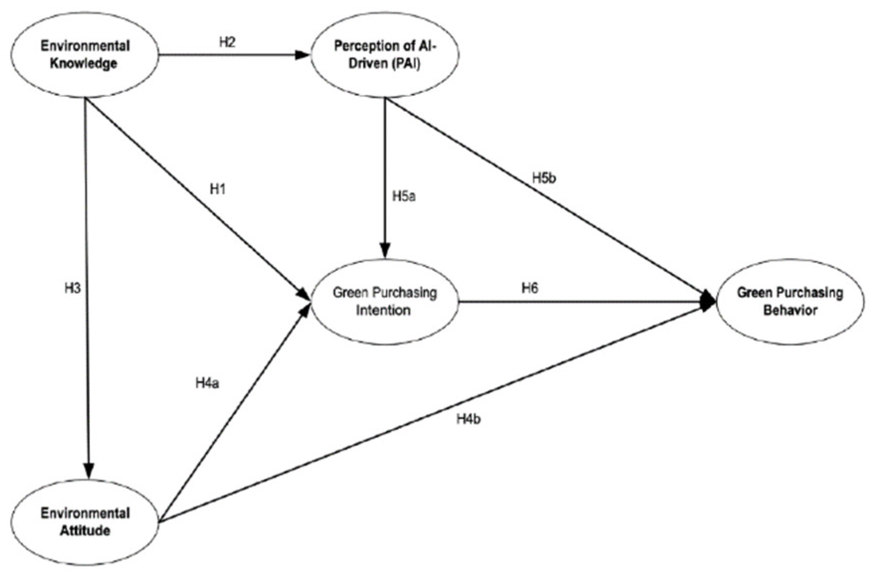
Table 1.
Convergent validity and reliability for the measurement model.
| Construct | Items | Loading Factor | CA | Rho A | CR | AVE |
| EAT | Eace1 | 0.652 | 0.818 | 0.833 | 0.869 | 0.528 |
| Eape1 | 0.802 | |||||
| Eapi1 | 0.797 | |||||
| Ears2 | 0.567 | |||||
| Easg3 | 0.721 | |||||
| Eass1 | 0.789 | |||||
| EK | Ekae1 | 0.788 | 0.769 | 0.785 | 0.844 | 0.521 |
| Ekek2 | 0.583 | |||||
| Ekls1 | 0.766 | |||||
| Ekse1 | 0.752 | |||||
| Ekue1 | 0.704 | |||||
| GPB | Gbbg1 | 0.846 | 0.854 | 0.855 | 0.895 | 0.631 |
| Gbcb1 | 0.742 | |||||
| Gbgm1 | 0.775 | |||||
| Gbll1 | 0.788 | |||||
| Gbpe2 | 0.818 | |||||
| GPI | Gpcp1 | 0.732 | 0.785 | 0.792 | 0.861 | 0.607 |
| Gpcs1 | 0.804 | |||||
| Gpib1 | 0.797 | |||||
| Gpis1 | 0.783 | |||||
| PAI | Paat2 | 0.734 | 0.766 | 0.761 | 0.843 | 0.520 |
| Paiu2 | 0.805 | |||||
| Papm1 | 0.568 | |||||
| Papu3 | 0.756 | |||||
| Pata3 | 0.721 |
Table 2.
Results of heterotrait monotrait ratio (HTMT).
| Construct | EAT | EA | GPB | GPI | PAI |
| EAT | |||||
| EK | 0.814 | ||||
| GPB | 0.749 | 0.566 | |||
| GPI | 0.721 | 0.600 | 0.808 | ||
| PAI | 0.396 | 0.360 | 0.376 | 0.398 |
Table 3.
Measurement Model Fitness.
| Fit Indices | Values |
|---|---|
| Chi-squared (χ2) | 1108 |
| SRMR | 0.074 |
| NFI | 0.799 |
| Rms Theta | 0.128 |
Table 4.
Results of Inner Variance Inflation Factor (VIF).
| Items | EAT | EK | GPB | GPI | PAI |
| EAT | 1.566 | 1.841 | |||
| EK | 1.000 | 1.790 | 1.000 | ||
| GPB | |||||
| GPI | 1.565 | ||||
| PAI | 1.148 | 1.124 |
Table 5.
Results of R square.
| Construct | R Square | R Square Adjusted |
| EAT | 0.436 | 0.435 |
| GPB | 0.553 | 0.550 |
| GPI | 0.373 | 0.369 |
| PAI | 0.077 | 0.075 |
Disclaimer/Publisher’s Note: The statements, opinions and data contained in all publications are solely those of the individual author(s) and contributor(s) and not of MDPI and/or the editor(s). MDPI and/or the editor(s) disclaim responsibility for any injury to people or property resulting from any ideas, methods, instructions or products referred to in the content. |
© 2025 by the authors. Licensee MDPI, Basel, Switzerland. This article is an open access article distributed under the terms and conditions of the Creative Commons Attribution (CC BY) license (http://creativecommons.org/licenses/by/4.0/).
Copyright: This open access article is published under a Creative Commons CC BY 4.0 license, which permit the free download, distribution, and reuse, provided that the author and preprint are cited in any reuse.


