
Submitted:
27 August 2025
Posted:
28 August 2025
You are already at the latest version
Abstract
For vertical take-off and landing (VTOL) control of distributed-propulsion fixed-wing UAVs exhibiting strong nonlinearity and aerodynamic/propulsive coupling, traditional linearization methods incur significant modeling errors in pitch-roll coupling and vortex interference scenarios due to neglected high-order nonlinearities, leading to inherent control law limitations. This study focuses on a non-tilting distributed-propulsion VTOL UAV featuring integrated airframe-propulsion design. Each of its four propulsion units contains six ducted rotors, arranged in tandem-wing configuration on both fuselage sides. A revised propulsion-aerodynamic coupling model was established and validated through bench tests and CFD data, enabling the design of an Incremental Nonlinear Dynamic Inversion (INDI) control architecture. The UAV dynamics model was constructed in Matlab/Simulink incorporating this revised model. An INDI-based attitude control law was developed with cascade controllers (angular rate inner-loop/attitude outer-loop) for VTOL mode, integrated with propulsion-system and control-surface allocation strategy. Digital simulations validated the controller's effectiveness and robustness. Finally, tethered flight tests with physical prototypes confirmed the method's applicability for high-precision control of strongly nonlinear distributed-propulsion UAVs.
Keywords:
distributed electric propulsion vehicle
; dynamics modelling
; incremental nonlinear dynamic inversion
; suspension experiments
1. Introduction
According to data released by the International Air Transport Association (IATA), carbon dioxide emissions from the aviation industry account for 2.5% of global total emissions and are increasing annually. Meanwhile, intensifying global competition is pressuring manufacturing enterprises to reduce energy costs. In response to growing international calls for carbon reduction in aviation, many aircraft manufacturers have shifted their production goals toward energy efficiency and low-carbon technologies [1,2,3,4].
Against the backdrop of current advancements in aviation emission reduction technologies, the distributed hybrid electric propulsion architecture has attracted significant attention as a promising solution to environmental challenges. This innovative propulsion system employs a conventional thermal engine to drive generators, which in turn power multiple distributed electric propulsion units (motor/propeller assemblies) along the aircraft’s wings or fuselage to perform primary or complete propulsion tasks [2,5,6,7,8]. Compared to traditional propulsion systems, this distributed layout not only reshapes the aerodynamic configuration of the aircraft, but also significantly increases the effective bypass ratio through flow field optimization, thus enhancing propulsion efficiency, reducing fuel consumption and pollutant emissions [5,6,7,8], and generating lower noise levels [9].Currently, most studies on distributed unmanned aerial vehicles (UAVs) adopt small-disturbance linearization analysis methods. However, during transitional flight phases, UAV dynamics evolve into multistate, coupled nonlinear models. Such strongly nonlinear systems are typically characterized by coupled high-order differential equations, requiring mathematical models that incorporate aerodynamic derivatives, inertial coupling terms, and propulsion system dynamics within a nonlinear state-space framework. Traditional linearized analysis methods, which neglect higher-order nonlinear coupling terms, result in significant modeling errors under typical conditions such as pitch-roll coupling and vortex interference, leading to fundamental flaws in control law design.
Meanwhile, as a vital carrier of modern aviation technology, UAV systems have demonstrated significant application value in national defense reconnaissance, ecological data collection, emergency supply delivery, and other fields [9,10]. In this context, enhancing mission execution accuracy in complex operational scenarios has become a focal point of research in flight control. As a core component of the flight control system, attitude regulation technology plays a decisive role in maintaining the operational stability of aerial platforms [9]. Optimizing this technology is not only crucial for achieving basic UAV performance metrics but also directly affects the reliability of aerospace equipment under extreme conditions. To ensure precise task execution by UAVs, extensive research has been conducted globally on attitude control methods [11,12,13,14]. Common methods include Proportional-Integral-Derivative (PID) control [13], backstepping control [14], sliding mode control [15], adaptive control [16], and Nonlinear Dynamic Inversion (NDI) [12]. However, these methods exhibit notable limitations when addressing multi-state coupled nonlinear systems: PID control struggles with tuning parameters in the presence of strong inter-channel coupling and lacks robustness; backstepping control is highly dependent on accurate dynamic models, leading to performance degradation under unmodeled dynamics; sliding mode control, although robust, suffers from chattering, which accelerates actuator wear; adaptive control allows online parameter tuning but is computationally intensive and often lags behind rapid system changes. These limitations fundamentally stem from the reliance of traditional control methods on accurate mathematical models. When confronted with the highly coupled nonlinear dynamics of transitional flight phases, control laws based on linear assumptions or simplified models cannot effectively compensate for time-varying aerodynamic parameters or nonlinear actuator saturation. While NDI simplifies control laws by mathematically inverting system dynamics to construct a linearized equivalent system for closed-loop control, it demands accurate models and invertible control input matrices, limiting its applicability [13].
The above analysis reveals that a key contradiction in traditional control approaches lies in their reliance on precise models versus the intrinsic nonlinearity and uncertainty of real-world systems. To address this issue, Incremental Nonlinear Dynamic Inversion (INDI) has garnered increasing interest in recent years. Derived from classical NDI theory [17,18], INDI introduces an incremental control strategy and utilizes sensor measurements to replace model-dependent components, significantly reducing dependence on precise system models while enhancing robustness. This method is particularly suitable for high-precision UAV control in complex dynamic environments [12,13,17,18].
In conclusion, distributed propulsion UAVs offer vast application prospects due to their unique configuration and performance advantages. However, this configuration also presents a series of unresolved issues in flight mechanics and control. To date, only limited studies have addressed the complex aerodynamic/propulsion coupling disturbances, and experimental validation on physical prototypes remains scarce. Therefore, this paper focuses on modeling the hovering dynamics of distributed propulsion UAVs, constructing aerodynamic and coupled propulsion component models, analyzing dynamic characteristics, and developing a reliable control allocation scheme to address these research gaps.
2. Dynamic Modeling
2.1. Definition and Transformation of Coordinate Systems
The UAV configuration studied in this work is illustrated in Figure 1a, which presents the aircraft state in hover mode. This is a distributed propulsion vertical take-off and landing (VTOL) fixed-wing UAV with a passive tilting mechanism. It features an integrated design of passive tilt, distributed propulsion, and a power-integrated fuselage. Each propulsion wing unit consists of six ducted rotors, with four propulsion wing units mounted in tandem on both sides of the fuselage. To ensure the general applicability of the model, both the ground coordinate system and the body-fixed coordinate system are defined. The ground frame is fixed to the Earth, with its origin at a certain point on the ground. Its vertical axis points toward the Earth’s center, while the other two axes and lie in the horizontal plane and are orthogonal to each other. Typically, the represents flight altitude. The body frame is fixed to the UAV, with its origin at the UAV’s center of mass. The lies within the plane of symmetry and points forward; the is perpendicular to the and points downward; the is perpendicular to the plane and points to the starboard wing.
Figure 1b presents a mechanical diagram of the propulsion wing unit. A dual control surface (upper and lower) is employed to achieve vertical takeoff and landing. During the VTOL process, the ducted jet flow must be deflected to generate vertical lift. Therefore, deflection vanes are added at the nozzle to change the airflow direction. In addition to the effect of the deflection vanes on the jet direction, the upper and lower control surfaces also contribute to deflection. The diagram includes quantities such as total lift (), total drag (), total moment (), resultant force magnitude (), and resultant force direction ().
The UAV’s attitude, position, and velocity are represented differently in different coordinate systems. Thus, the transformation relationships between coordinate systems must be clarified before establishing motion equations. The transformation from the ground frame to the body frame is expressed as:
Taking the inverse of the above gives the transformation matrix from the body frame to the ground frame.
2.2. UAV Motion Equations
This section derives the motion equations of the UAV. The focus of this study is on the vertical takeoff, landing, and hovering phases; therefore, lateral-directional motion equations are omitted. Under the assumption of coordinated horizontal flight (no sideslip), the nonlinear dynamics of the fixed-wing UAV are modeled in continuous time:
Firstly, the following assumptions need to be given as UAVs are affected by complex factors in the actual flight environment:
1) The Earth is taken as an inertial reference frame, assumed non-rotating and with negligible curvature. Gravitational acceleration is constant.
2) The UAV is treated as a rigid body with no deformation under external forces, and its center of mass is fixed.
3) The UAV’s mass and moment of inertia are constant.
Based on the above assumptions and a force analysis of the UAV, the Newton-Euler equations yield:
Where: F is the total external force, m is the mass, V is the velocity vector, M is the total external moment, and H is the angular momentum.
Expanding (2), we obtain the translational motion differential equations:
Expanding (3), we obtain the rotational motion differential equations:
Retaining only the equations related to longitudinal motion and rearranging, we derive the UAV’s longitudinal dynamic model:
where is the flight path angle, is the angle of attack, q is the pitch rate, is the moment of inertia, and the pitch angle .
2.3. Propulsion Wing and Deflection Surface System Model
The distributed electric propulsion VTOL UAV studied in this work incorporates deflection surfaces downstream of the ducted propulsion wings. These surfaces deflect high-speed jets from the propulsion system to generate aerodynamic forces for VTOL, reducing energy consumption during vertical operations. Moreover, by deflecting the thrust vector via these surfaces, aircraft maneuverability is improved. This section presents the propulsion wing–deflection surface unit model under powered input, followed by system-level modeling.
Zhao. et al. [3] derived the lift model using momentum theory as follows:
Where is the freestream angle of attack, is the thrust correction factor, is the deflection vane flow angle, is the duct flow deflection angle, is the rotor disk area, and is the freestream cross-sectional area. The first term on the right represents thrust deflection by the deflection surface, the second term is the lift from freestream flow without power input, and the third term accounts for volume blockage effects by the jet stream.
Similarly, the axial thrust generated by the unit is:
The first term represents the axial component of deflected duct thrust, the second term is drag under no power input, and the third term is additional drag due to the jet flow. Notably, when freestream velocity is zero (i.e., in hover), the deflection surface mainly serves to redirect thrust.
The aerodynamic model of the power wing-induced airfoil unit is obtained from the previous section, and the overall distributed power wing-induced airfoil system is now modeled. Wang Kelei et al. [2] proposed that the spreading distribution of the power wing-induced airfoil units mainly brings two effects: 1) the aerodynamic coupling effect between the propulsion units arranged along the spreading direction, and this interaction will significantly change the inlet environment parameters of each power module, such as the flow field velocity and the airflow incidence angle and other parameter characteristics. Due to this interference effect, the thrust output and energy conversion efficiency of each unit of the distributed propulsion system will have a 6-8% degradation. 2) Under the interference condition of wingtip vortex field, the distribution law of lift along the spreading direction of the distributed propulsion airfoil and its fluctuation range are highly similar to that of the conventional airfoil. For the power loss due to adjacent power pumping induction, it can be corrected by the thrust correction factor. For the effect of the change of lift distribution in the spreading direction, the following corrections can be made to the distributed power wing-induced airfoil model with reference to the relationship between the aerodynamic characteristics of the three-dimensional airfoil and the two-dimensional airfoil:
where: L is the total lift of the corrected system; N is the number of unit spreading distribution; is the unit lift; is the lift correction factor.
Similarly, due to the change in lift, there is a change in induced drag, so the system thrust can be corrected as:
where: T is the modified total system thrust; is the unit thrust; is the wing spread ratio; and e is the Oswald factor.
2.4. Propulsion Wing Unit Bench Test
Although lift and drag models have been derived, UAVs exhibit nonlinear, strongly coupled, and uncertain parameter characteristics, making precise modeling difficult. Thus, a bench test was conducted to calibrate the mathematical model based on measured lift characteristics. Figure 2 shows the schematic of the bench test system; Figure 3 presents the actual experimental setup.
The propulsion wing unit was mounted on a balance using connectors, with varying deflection angles and throttle settings. The balance output was recorded and transformed into lift characteristics using coordinate transformation. The resulting lift characteristics are shown below.
3. INDI Controller Design and Simulation Verification
3.1. INDI Controller
According to Liu. et al.[18], Incremental Nonlinear Dynamic Inversion (INDI) is essentially a feedback linearization method that compensates nonlinear and coupling terms in the system to achieve a decoupled linear transfer relationship. In this section, the INDI control law will be given according to the literature[12].
Consider a nonlinear system:
where x is the state vector, u is the input vector, and y is the output vector. The conventional NDI control law is:
Where: v denotes the desired output response of the system. It can be seen that conventional NDI requires an accurate global nonlinear model, but in distributed systems, (Coriolis force, gyroscopic effect, etc.) it is difficult to model accurately. Its robustness deteriorates when there are parameter ingressions and uncertainties. And according to the literature[12,19,20,21], the control law of INDI is:
where and are the previous state and control input, and is the estimated control effectiveness for . From the above equation, it can be seen that the INDI control law does not depend on , the relevant information of the controlled object model is replaced by the filter measurements that can be made. Therefore, INDI control has a low dependence on the model and is more robust to model uncertainties and disturbances. The longitudinal INDI control system is constructed from the above equation as Figure 5 show:
The overall system includes an altitude linear controller and an attitude INDI controller.
In order to eliminate the static error of altitude tracking, a linear PI controller is used in the altitude outer loop, whose inputs are the desired altitude and the current altitude, and the altitude controller calculates the error between them and outputs the longitudinal velocity command in the ground coordinate system. In addition, to enhance the robustness of the system to atmospheric perturbations (e.g., ground effects) and sensor drift, an auxiliary feedback to the estimated rate of change of altitude is also introduced. And then, together with the horizontal velocity command , it is fed into the velocity controller, which uses a linear gain structure to produce rejection of the velocity error and outputs the desired rate of change of velocity for acceleration level regulation. The current estimated velocity is used as a feedback signal during the control process to calculate the desired acceleration and compared to produce an error signal input to the attitude control module.
The attitude control system needs to stabilize the tracking of the attitude angle command output from the front circuit system, in order to ensure the tracking accuracy, the attitude control system is divided into the attitude angle outer loop and the angular velocity inner loop. The attitude angle outer loop is composed of a linear PID controller that inputs the attitude angle corresponding to the desired acceleration ( solved by the control matrix) and outputs the desired angular velocity, while the angular velocity inner loop adopts INDI control, and the core role of the inner loop INDI is to solve the angular acceleration command by using the current control effectiveness model (i.e., the real-time estimated control allocation matrix , : which represents the effect of the control inputs on the angular acceleration of the airframe) and the sensor data. Pseudo-inverse control quantities to improve robustness to aerodynamic disturbances by directly compensating for disturbances through the dynamic inverse model. The input feedback signal is the angular acceleration error. Control mixing and control matrix solving form the control system mixer, the input signal is the pseudo-inverse control quantity output from INDI, and the pseudo-inverse signal is solved into the thrust increment , and rudder deflection commands of 4 power wing units (one group on the same side) through the control allocation matrix, so as to realize the attitude control of the UAV.
This control system architecture realizes the problem of controlling the distribution and strong coupling characteristics of a distributed electric propulsion multi-input system through hierarchical decoupling and introducing the anti-jamming capability of the INDI inner loop, combined with the real-time solving of the control allocation of distributed power.
3.2. Digital Simulation Verification
MATLAB 2022b and Simulink 5.1 are used to build the UAV simulation system, shown in Figure 6.
The simulation system includes the UAV model, mixed controller, environment model, control bus system, and oscilloscope. The UAV model comprises a 6-DOF model, aerodynamic model, and propulsion model. The Commander state flow initializes and manages simulation conditions, while oscilloscopes record real-time states. The simulation initial conditions and simulation state settings are shown in Table 1.
Table 2 summarizes UAV performance parameters, based on CFD and bench tests. To verify the designed INDI controller, simulations were conducted under disturbance and actuator failure scenarios.
3.2.1. Disturbance Rejection Simulation
To match typical electric motor dynamics of small UAVs, a first-order inertial element with time constant is used. The simulation investigates vertical transition from takeoff to hover. Initially, the UAV rests on the ground with a pitch angle of , then ascends vertically to and hovers. To verify robustness, a pitch disturbance is added after hovering stabilizes. Figure 7 shows flight states.
The UAV is able to take off vertically smoothly under the designed control scheme, with an altitude overshoot of no more than , a pitch angle fluctuation of or less and throttle levels within control bounds (dt3 and dt6 shown as representative). X-axis speed fluctuates is within during takeoff, while Y-axis speed remains zero, confirming vertical lift-off capability. After applying disturbance at , height remains steady, speed deviation is witnin , pitch within , all recovering within —demonstrating strong robustness.
The longitudinal control and anti-jamming capability of the UAV was verified above. Further, to test attitude control, a yaw command is issued after stabilization, followed by a roll command. A lateral disturbance is continuously applied. Figure 9 shows flight states.
As shown in the Figure 8, after applying lateral and directional disturbance moments during stable hover, both roll and yaw angles promptly return to stability with fluctuations not exceeding . Furthermore, when attitude angle commands were applied at and respectively, the UAV accurately tracked the commands with less than overshoot and steady-state error. Control surface deflections remained within acceptable limits while altitude maintained stability throughout. These results validate the INDI controller’s precise attitude control and strong disturbance rejection capabilities.
3.2.2. Power Failure Simulation
In actual flight, propulsion failure represents a typical fault that distributed-propulsion UAVs must address. The ability to rapidly recover attitude stability during sudden propulsion failure serves as a critical metric for evaluating controller robustness. As previously described, the six thrusters are divided into two groups (Thrusters 1-3 and 4-6) in the simulation. This test verifies the strong robustness of the INDI controller by deactivating one thruster in each group. Specific procedure: After achieving stable hover, Thruster 2 was deactivated at , followed by Thruster 5 at , with all thrusters reactivated at . Simulation results are shown in Figure 9.
The UAV’s pitch angle exhibits fluctuations within after propulsion failure. Nevertheless, the controller enables rapid command tracking, maintaining post-recovery tracking error below . Altitude remains stable throughout, while forward velocity experiences approximately fluctuations during failure (within acceptable limits), recovering to zero promptly after propulsion restoration to reestablish hover. Figure 9d demonstrates that after single-thruster failure, the remaining thrusters respond rapidly with maximum throttle commands not exceeding 0.83. This confirms maintained control redundancy during single-point failures and validates the strong robustness of the INDI (Incremental Nonlinear Dynamic Inversion) controller.
4. Suspension Test and Conclusion
For actual flight validation where parameters (e.g., moment of inertia, thrust efficiency) differ from simulation, tether-assisted hanging tests were conducted to verify attitude control. The physical platform parameters matched those in Table 2, except the reference pitch angle was set at due to center-of-gravity configuration. Figure 10 shows the tethered system hardware: UAV, suspension frame, remote emergency cutoff switch, and ground station system (including communication link, real-time kinematic (RTK) base station, etc.). The UAV was suspended via steel cables ensuring exclusive longitudinal tension. Flight states were monitored and recorded by the ground station, while the emergency cutoff switch enabled immediate braking during contingencies. Procedure: (1) Elevate tethered UAV to preset altitude; (2) After ground station unlocking, operator-controlled takeoff; (3) Transition to hover mode at target altitude; (4) Automatic data logging by flight control system. Tests proceeded under wind-disturbed conditions to concurrently evaluate disturbance rejection. Three phases comprised: a) Hover tests validating VTOL capability and flight logic; b) Forward-impulse tests assessing attitude controller’s disturbance rejection; c) Propulsion-failure tests verifying robustness of the INDI (Incremental Nonlinear Dynamic Inversion) controller.
4.1. Hover Test
The hover test lasted 70 seconds. As shown in Figure 11a, the UAV takes off manually from a height of 0.8 m. At , the system switches to stabilized mode, during which a sudden pitch-down command of approximately occurs. The INDI controller compensates, stabilizing the aircraft and allowing it to ascend. At , the UAV switches to altitude-hold mode with altitude variations within . From 30 to , the UAV maintains hover before switching back to manual mode and ascending for the next test. Throughout the process, the UAV remains stable. Figure 11b shows that the pitch angle closely follows the command, with fluctuations within , excluding mode transitions. Figure 11c indicates continuous roll angle fluctuations within due to wind interference. Roll command tracking shows a delay, acceptable for the UAV’s limited control authority. Figure 11d shows yaw changing from to , initially offset due to mechanical asymmetry and gradually corrected after takeoff. Some overshoot and latency are observed due to wind and control limitations. Figure 11e indicates throttle usage never exceeds 0.7 (maximum defined as 1), suggesting sufficient control margin.
4.2. Forward Impulse Test
Surge test data (Figure 12) indicate three consecutive tethered surges initiated at , , and respectively. Constrained by the tether mechanism, forward velocity was limited to . Pitch response curves (Figure 12b) demonstrate rapid command tracking with low latency, maintaining deviation during surges. Height variations during each surge event remained (Figure 12c). Throttle commands never exceeded 80% throughout the test (Figure 12d), with thruster differential magnitude merely 0.05 (full-scale reference: 1.0) during surges.
4.3. Power Failure Test
Following hover and surge tests validating the INDI controller’s flight logic and disturbance rejection, propulsion-failure tests were conducted to evaluate robustness. In these tests, one thruster unit in each of the left-rear (L-R) and right-front (R-F) positions was deactivated (six units total), while UAV flight states were monitored. Safety measures included tethering the UAV at an increased altitude of . The procedure involved a vertical takeoff to hover, triggering the thruster failure, transitioning to operator-controlled manual mode, and recording the flight parameters.
Figure 13 shows at during stable hover, sudden thruster failure caused altitude drop due to lift deficit. Subsequent throttle increase restored altitude while maintaining pitch oscillations .Differential throttle commands emerged in failure-affected thruster groups (Figure 13d) to counteract disturbance moments from asymmetric thrust. During surge simulation initiated at , pitch angle maintained precise command tracking despite acceptable latency/error, with maximum throttle at 80% confirming control margin.
Suspension tests demonstrate: The INDI controller achieves disturbance rejection in physical flights, maintains control accuracy under dual modes, and preserves attitude stability plus maneuverability post-failure. This verifies bounded-disturbance robustness with control redundancy ensuring operational reliability.
5. Conclusions
This study addresses the vertical takeoff, landing, and hovering control of distributed propulsion fixed-wing UAVs. A modified modeling approach is proposed, employing momentum theory to derive a propulsion–aerodynamic coupling model under powered conditions. Additionally, aerodynamic corrections are introduced to account for differences between 3D wings and 2D airfoils. Wind tunnel and bench test results are used to calibrate the mathematical lift model.
Considering the multi-variable, nonlinear, strongly coupled, high-order, and uncertain characteristics of the system, an INDI-based control scheme is developed. This approach reduces dependency on precise UAV models and enhances robustness. Simulation tests under wind disturbance confirm feasibility, and suspension experiments demonstrate precise attitude control and strong disturbance rejection. Furthermore, motor failure tests validate the robustness of the INDI controller.
Future work will focus on extending the INDI-based control strategies to different flight conditions and conducting full-scale flight tests for validation.
Author Contributions
Conceptualization, Q.Z. and Y.Z.; methodology, Q.Z. and R.W.; software, Y.Z.; validation, Y.Z.; formal analysis, Q.Z. and Y.Z.; investigation, Y.Z.; resources, Y.Z.; data curation, Q.Z. and Y.Z.; writing—original draft preparation, Y.Z.; writing—review and editing, Q.Z.; visualization, Q.Z. and Y.Z.; supervision, Q.Z.; project administration, R.W.; funding acquisition, Z.Z. All authors have read and agreed to the published version of the manuscript.
Funding
This research was funded by the Pre-Research Project for Equipment Development (Program No.50911040803) and Aeronautical Science Foundation of China (Program No.2024Z006053001).
Data Availability Statement
Data is contained within the article or supplementary material.
References
- She Y. Fu K. Diao B. Sun M. Experimental Validation of a Rule-Based Energy Management Strategy for Low-Altitude Hybrid Power Aircraft. Aerospace 2025, 12, 758. [CrossRef]
- WANG Kelei, ZHOU Zhou, GUO Jiahao, et al. Propulsive/aerodynamic coupled characteristics of distributed-propulsion-wing during forward flight[J]. Hangkong Xuebao/Acta Aeronautica et Astronautica Sinica, 2024, 45(2): 128643. [CrossRef]
- ZHAO Qingfeng, ZHOU Zhou, LI Minghao, et al. Propulsion/aerodynamic coupling modeling for distributed-propulsion-wing with induced wing configuration[J]. Hangkong Xuebao/Acta Aeronautica et Astronautica Sinica, 2024, 45(10): 150–164. [CrossRef]
- Xiao N. Qiao X. Chen X. Li B. Reliability Analysis of Multi-Rotor Drone Electric Propulsion System Considering Controllability and FDEP. Drones, 2025, 9(8), 572. [CrossRef]
- WANG K, ZHOU Z. Aerodynamic design, analysis and validation of a small blended-wing-body unmanned aerial vehicle[J]. Aerospace, 2022, 9(1): 36. [CrossRef]
- ZHU Bingjie, YANG Xixiang, ZONG Jian’an, DENG Xiaolong. Review of distributed hybrid electric propulsion aircraft technology[J]. ACTA AERONAUTICAET ASTRONAUTICA SINICA, 2022, 43(7): 25556. [CrossRef]
- Zhuoyuan LI, Xudong YANG, Kai SUN, Junhui XIONG, Shuai SHI. Aerodynamic configuration of distributed ducted fan with complex strong interference effect and performance influence[J]. Acta Aeronautica et Astronautica Sinica, 2025, 46(3): 130805. [CrossRef]
- GUO J, ZHOU Z. Multi-objective design of a distributed ducted fan system[J]. Aerospace, 2022, 9(3): 165. [CrossRef]
- Raza W. Stansbury RS. Noise Prediction and Mitigation for UAS and eVTOL Aircraft: A Survey. Drones, 2025, 9(8), 577. [CrossRef]
- HE Hai-yang, ZHAO Zhen-gen, KONG Feiet al. Longitudinal control of fixed-wing UAV based on deep reinforcement learning[J]. Journal of Beijing University of Aeronautics and Astronautics,2024. [CrossRef]
- Agnes STEINERT, Stefan RAAB, Simon HAFNER, Florian HOLZAPFEL, Haichao HONG, From fundamentals to applications of incremental nonlinear dynamic inversion: A survey on INDI–Part I. Chinese Journal of Aeronautics, 2025, 103553. [CrossRef]
- Rui Wang, Zhou Zhou, Mihai Lungu, Linfang Li, PSD INDI and wake gradient based control of high aspect ratio UAVs’ close formation flight. Aerospace Science and Technology, 2025, 162: 110198. [CrossRef]
- YU Z Q, ZHANG Y M, JIANG B. PID-type fault-tolerant prescribed performance control of fixed-wing UAV[J]. Journal of Systems Engineering and Electronics, 2021, 32(5): 1053–1061. [CrossRef]
- ZHENG F Y, ZHEN Z Y, GONG H J. Observer-based backstepping longitudinal control for carrier-based UAV with actuator faults[J]. Journal of Systems Engineering and Electronics, 2017, 28(2): 322–377. [CrossRef]
- LEE S K, LEE J H, LEE S M, et al. Sliding mode guidance and control for UAV carrier landing[J]. IEEE Transactions on Aerospace and Electronic Systems, 2018, 55(2): 951–966. [CrossRef]
- Rui Wang, Zhou Zhou, Xiaoping Zhu, Zhengping Wang. Responses and suppression of Joined-Wing UAV in wind field based on distributed model and active disturbance rejection control. Aerospace Science and Technology, 2021, 115: 106803. [CrossRef]
- SUN Shuang, DONG Hualong, ZHAO Ziqing, et al. Single rotor failure control of tilt-rotor eVTOL based on Incremental Nonlinear Dynamic Inversion[J]. Propulsion Technology, 2025,. [CrossRef]
- LIU Shuangxi, LIN Zehuai, LIU Wei, et al. Transition mode control scheme of tilt rotor UAV based on INDI[J]. Hangkong Xuebao/Acta Aeronautica et Astronautica Sinica, 2024, 45(17): 236–250. [CrossRef]
- STEFFENSEN R, STEINERT A, SMEUR E J J. Nonlinear dynamic inversion with actuator dynamics: an incremental control perspective[J]. Journal of Guidance, Control, and Dynamics, 2022, 46(4): 709–717. [CrossRef]
- LIU Z, ZHANG Y, LIANG J J, et al. Application of the improved incremental nonlinear dynamic inversion in fixed-wing UAV flight tests[J]. Journal of Aerospace Engineering, 2022, 35(6): 04022091. [CrossRef]
- AHMADI K, ASADI D, NABAVI-CHASHMI S Y, et al. Modified adaptive discrete-time incremental nonlinear dynamic inversion control for quadrotors in the presence of motor faults[J]. Mechanical Systems and Signal Processing, 2023, 188: 109989. [CrossRef]
Figure 1.
Schematic layout of the UAS: (a) hover mode. (b) propulsion wing unit.
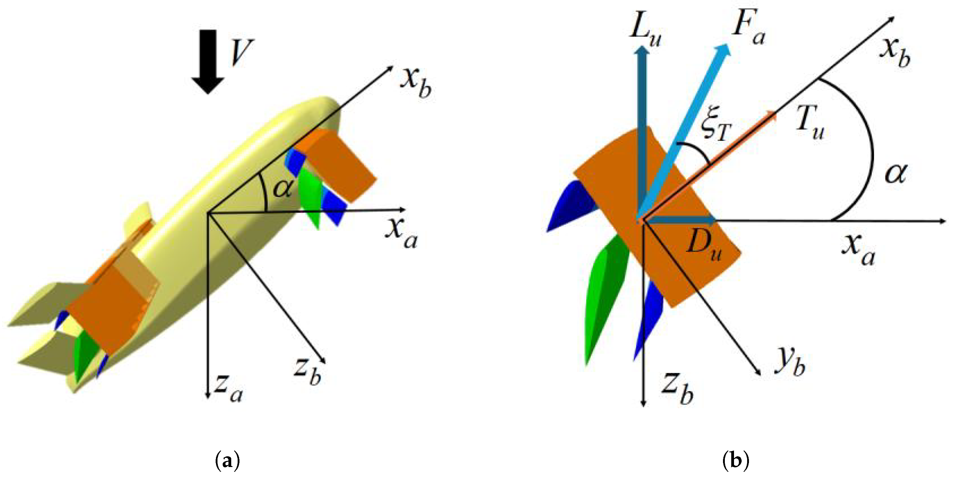
Figure 2.
Schematic diagram of the bench test system.
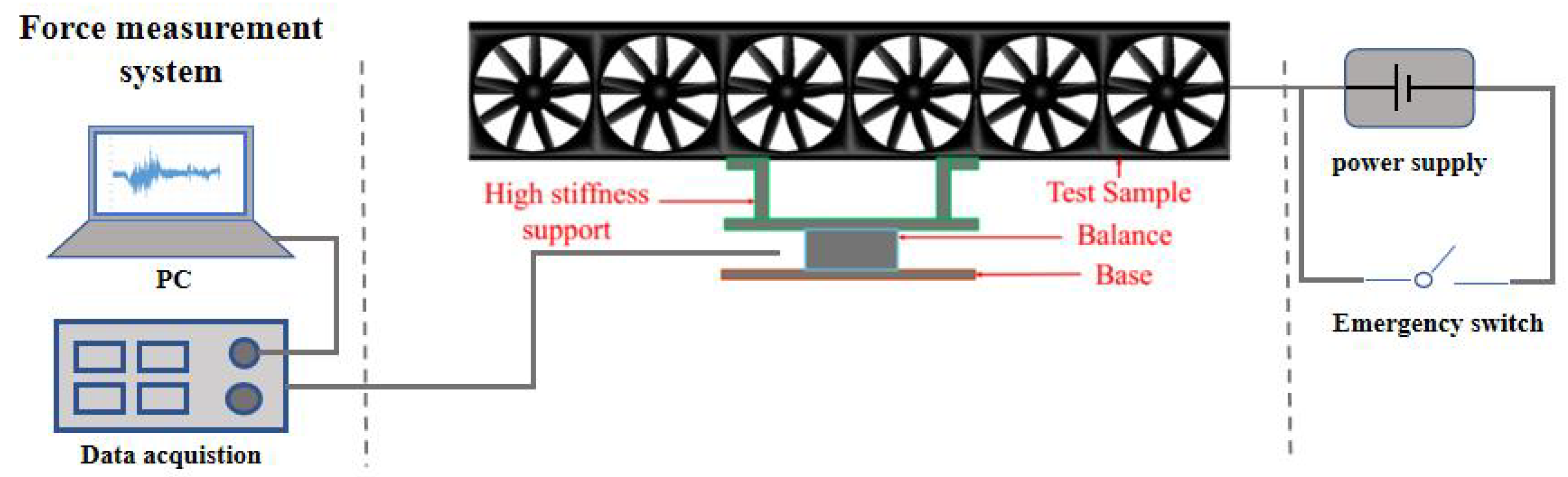
Figure 3.
Partial certification of bench test systems.
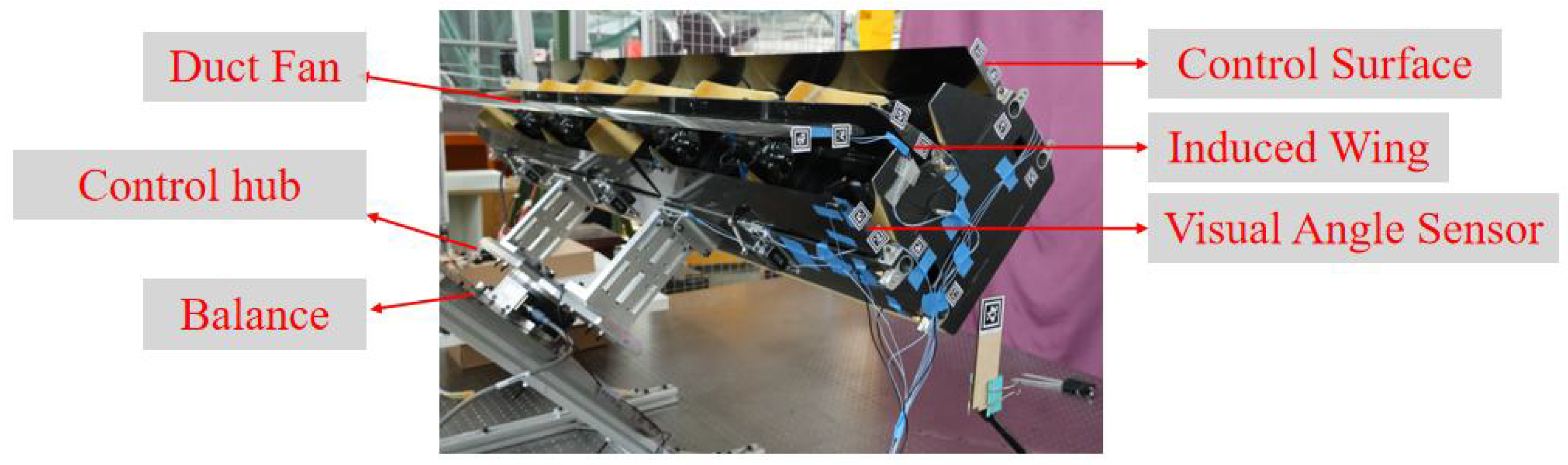
Figure 4.
Lift and Rudder Effect Characteristics: (a) Lift. (b) Rudder Effect.
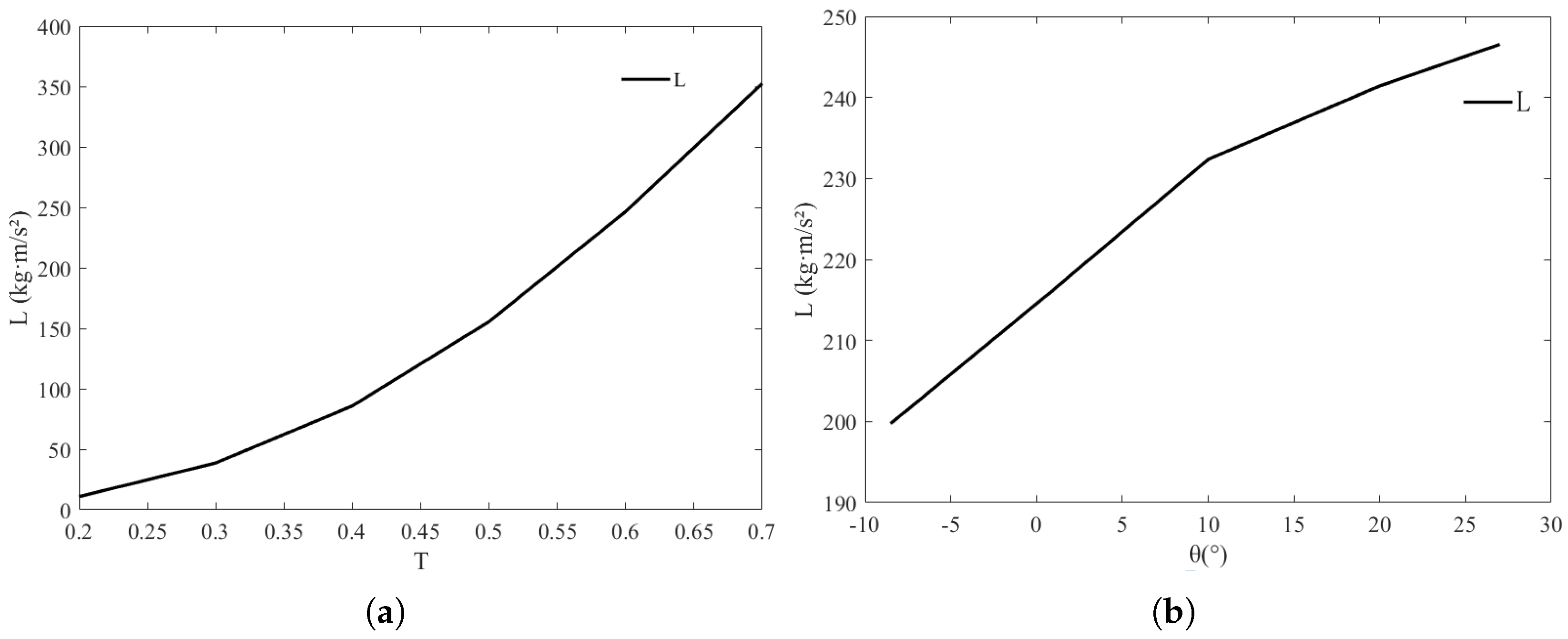
Figure 5.
Vertical control system.
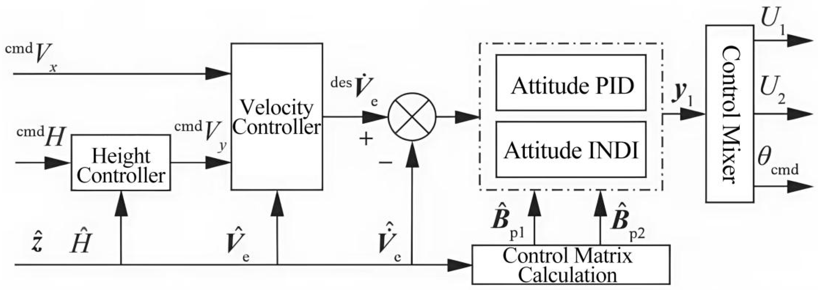
Figure 6.
digital simulation system.
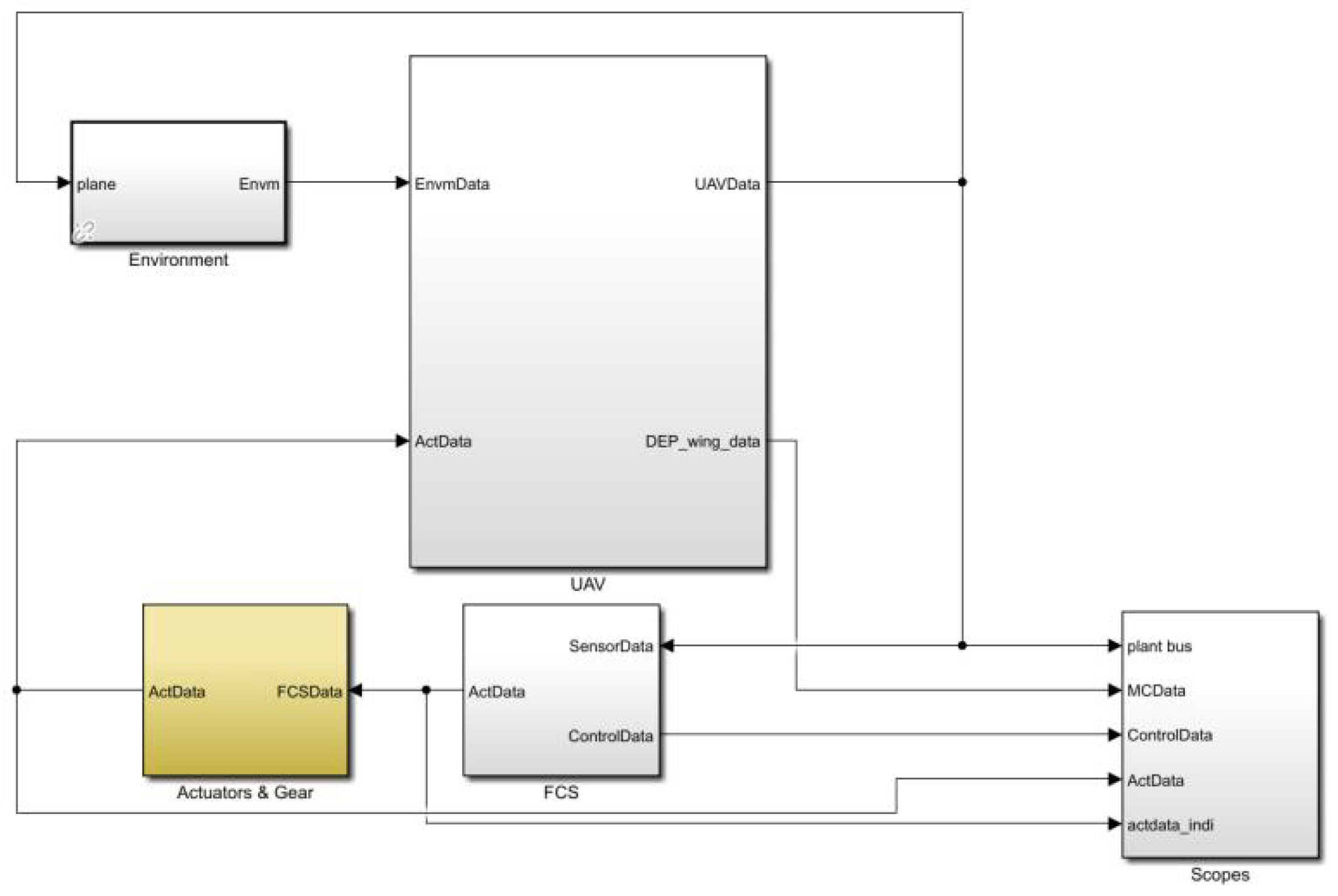
Figure 7.
Simulation state: (a) Velocity. (b) Height. (c) Pitch. (d) Throttle.
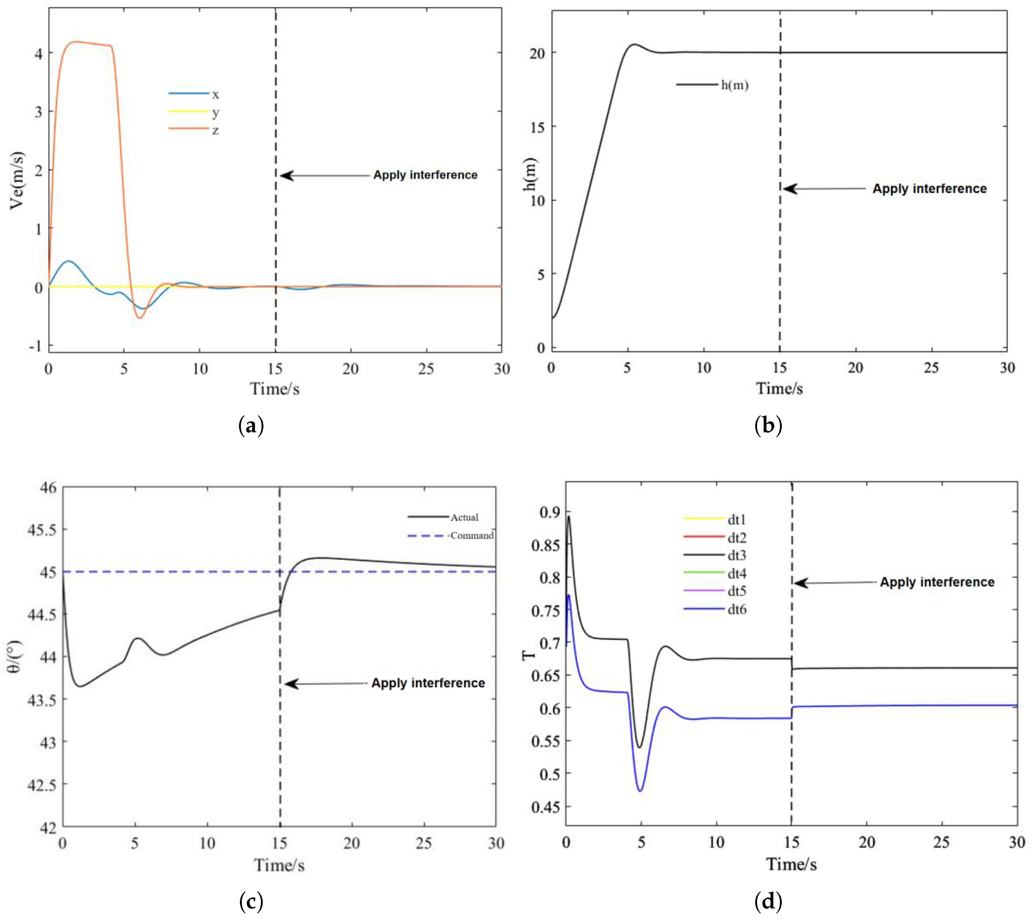
Figure 8.
Simulation state: (a) Height. (b) Yaw. (c) Roll. (d) Rudder angle.
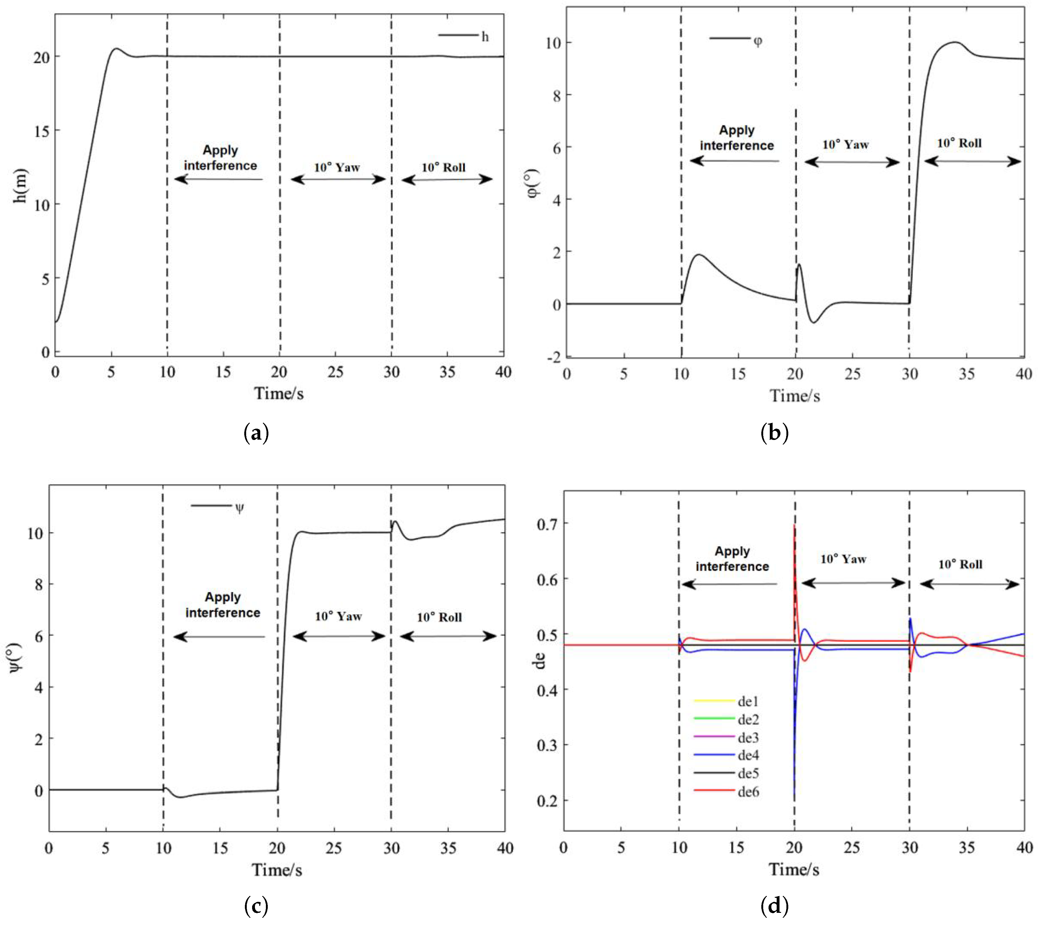
Figure 9.
Simulation state: (a) Height. (b) Pitch. (c) Velocity. (d) Throttle.
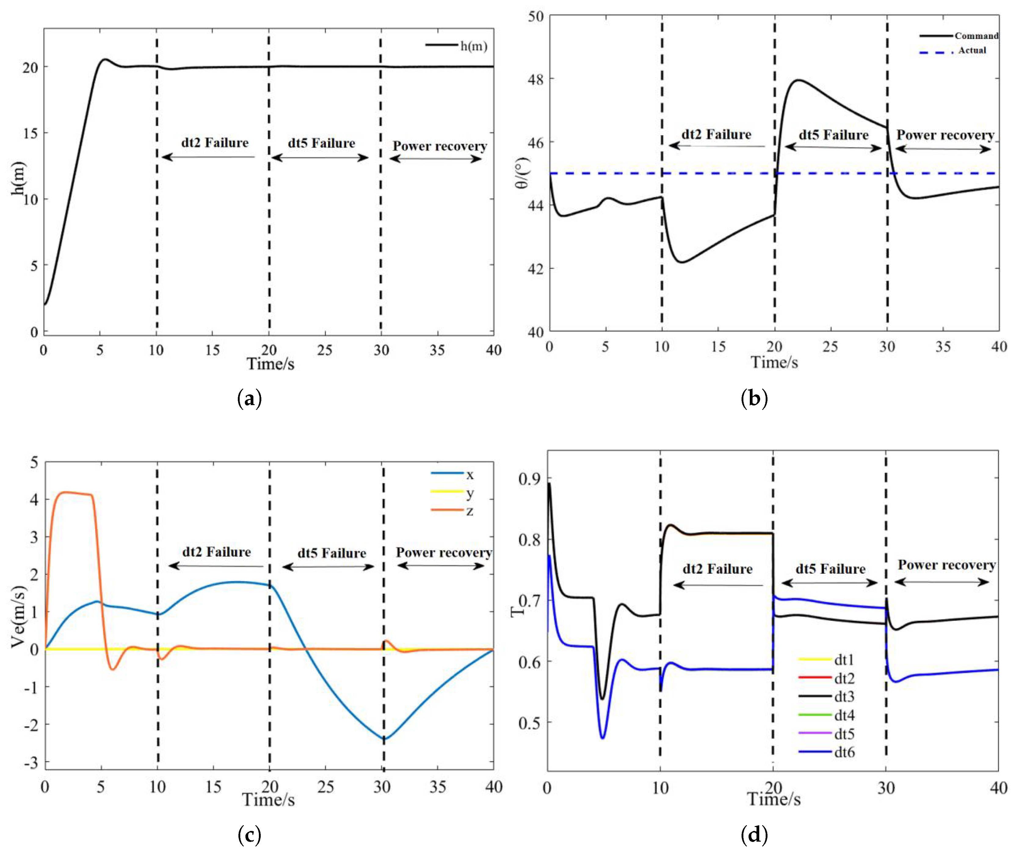
Figure 10.
Suspension diagram.
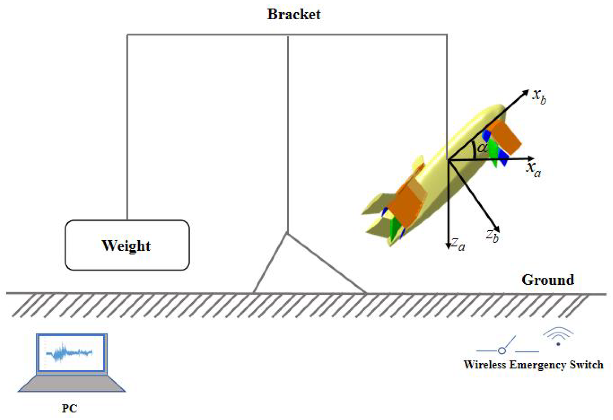
Figure 11.
Simulation state: (a) Height. (b) Pitch. (c) Yaw. (d) Roll. (e) Throttle.
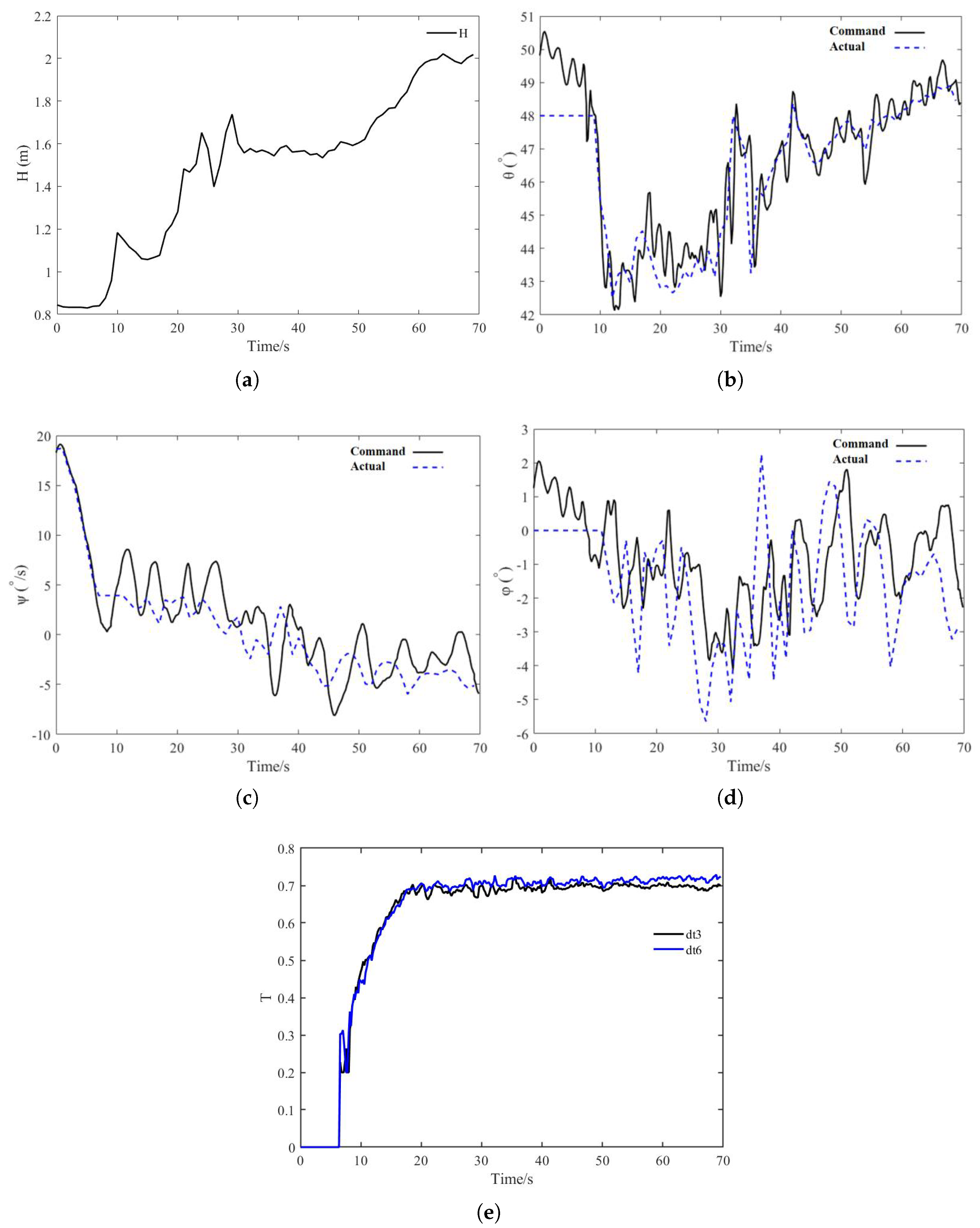
Figure 12.
Simulation state: (a) Vx. (b) Pitch. (c) Height. (d) Throttle.
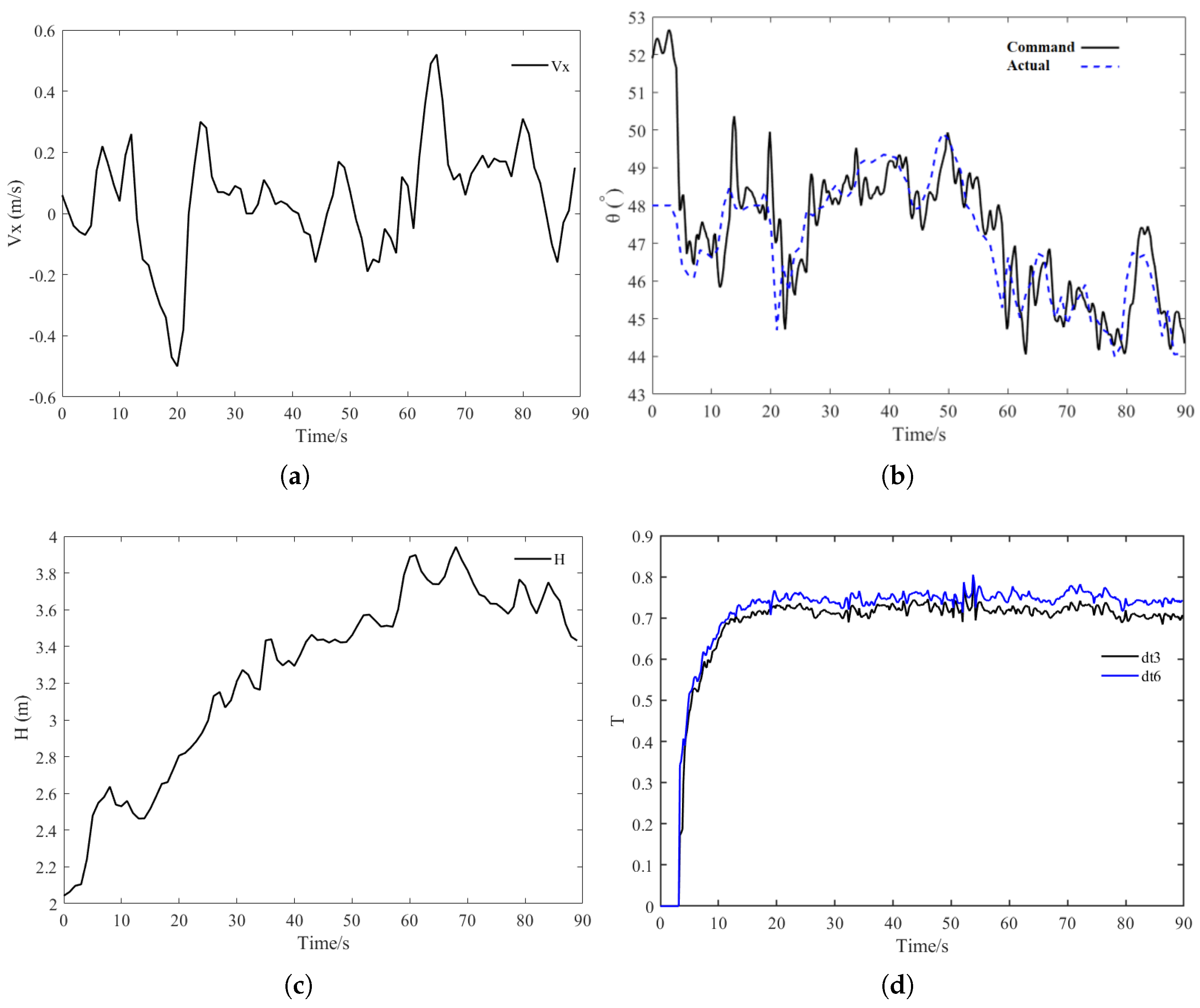
Figure 13.
Simulation state: (a) Height. (b) Pitch. (c) Vx. (d) Throttle.
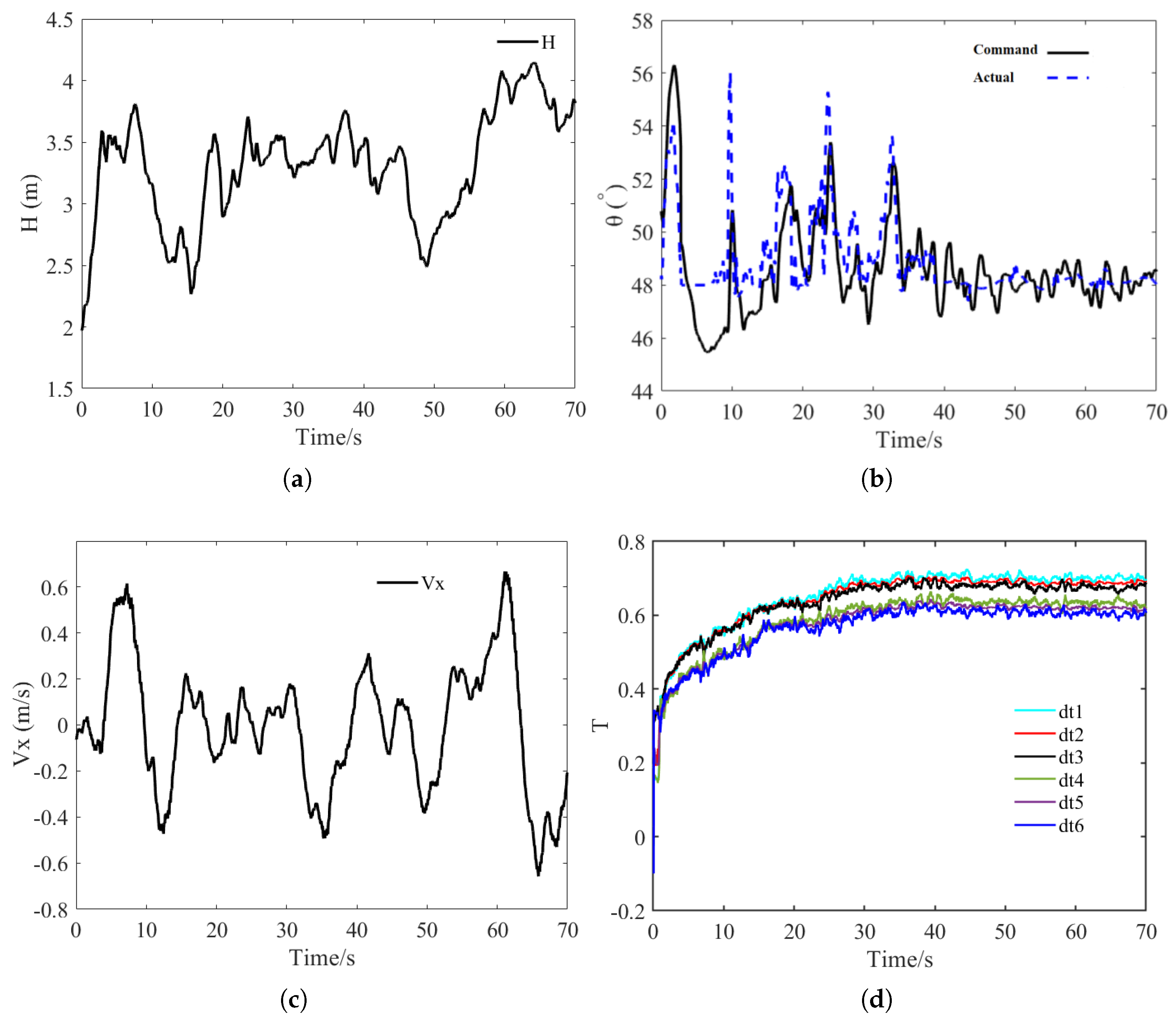

Table 1.
Simulation settings.
| Parameter | Initial conditions | Target setting |
|---|---|---|
| Height/m | 2 | 20 |
| Attitude angle/° | (0, 45, 0) | (10, 45, 10) |
| Wind interference/ | (50, 50, 50) | |
| Induced wing declination/° | 54 | |
| Rudder declination/° | 27 | |
Table 2.
UAV Performance Parameters.
| Parameters | Numerical value |
|---|---|
| Mass / kg | 100 |
| Wingspan / m | 3 |
| Fuselage length / m | 2 |
| Duct Diameter / m | 0.25 |
| / () | 53.6 |
Disclaimer/Publisher’s Note: The statements, opinions and data contained in all publications are solely those of the individual author(s) and contributor(s) and not of MDPI and/or the editor(s). MDPI and/or the editor(s) disclaim responsibility for any injury to people or property resulting from any ideas, methods, instructions or products referred to in the content. |
© 2025 by the authors. Licensee MDPI, Basel, Switzerland. This article is an open access article distributed under the terms and conditions of the Creative Commons Attribution (CC BY) license (http://creativecommons.org/licenses/by/4.0/).
Copyright: This open access article is published under a Creative Commons CC BY 4.0 license, which permit the free download, distribution, and reuse, provided that the author and preprint are cited in any reuse.


