Submitted:
27 August 2025
Posted:
28 August 2025
You are already at the latest version
Abstract
Anaerobic codigestion of organic residues is a proven strategy for enhancing methane recovery. However, the complexity of microbial interactions and variability in operational conditions make it difficult to estimate methane concentration in real time, particularly in rural contexts. This study developed a multiple linear regression model to predict methane concentration using operational data and microbial community profiles derived from 16S rRNA gene sequencing. The system involved the codigestion of cassava by-product and pig manure in a two-phase anaerobic reactor. Predictor variables were selected through a hybrid approach combining statistical correlation with microbial functional relevance. The final model, trained on 70% of the dataset, demonstrated satisfactory generalization capability on the 30) test set, achieving a coefficient of determination (R²) of 0.92 and a mean absolute error (MRE) of 6.50%. Requiring only a limited set of inputs and minimal computational resources, the model offers a practical and accessible solution for estimating methane levels in decentralized systems. The integration of microbial community data represents a meaningful innovation, improving prediction by capturing biological variation not reflected in operational parameters alone. This approach can support local decision-making and contribute to Sustainable Development Goal 7 by promoting reliable and affordable technologies for clean energy generation in rural and resource-constrained settings.
Keywords:
codigestion
; metagenomics
; biogas
; MLR
1. Introduction
The Valle del Cauca region is one of Colombia’s most active agro-industrial areas, combining high agricultural productivity with unique ecological richness. The territory is sustained by ecosystems that range from coastal plains to montane forests, which support both biological diversity and productive capacity. It ranks as the third-largest producer and consumer of pork in the country, with a reported output of 88105 tons in 2023, equivalent to 15.6% of national production, and an average pig population exceeding 396000 animals [1,2]. This sector generates large volumes of pig manure (PM) that require appropriate handling to prevent environmental and public health risks. Another productive activity with growing regional relevance is cassava cultivation, which covered approximately 564 hectares in 2020, yielding a total of 9888 tons of fresh roots [1]. During starch extraction, each kilogram of cassava generates about 0.2 kilograms of starch, 0.65 kilograms of fibrous residue (cassava dregs (CD)), and between five and seven liters of wastewater [3]. Based on these ratios, the estimated annual generation of by-products in the region reaches nearly 6427 tons, most of which are not currently valorized [4,5,6].
To address the increasing accumulation of organic residues from pig farming and cassava processing, anaerobic digestion (AD) has been promoted in rural areas of Valle del Cauca as a strategy for energy recovery and waste management. In these settings, one phase tubular biodigesters are commonly employed due to their affordable construction, ease of installation and minimal infrastructure requirements, making them particularly attractive to smallholder producers [7,8]. AD is a biologically mediated process in which organic matter is sequentially transformed into methane through four main stages, each driven by specific microbial groups. In the hydrolysis phase, hydrolytic bacteria degrade complex macromolecules such as carbohydrates, proteins and lipids into soluble monomers. These compounds are then metabolized by acidogenic bacteria during acidogenesis, producing volatile fatty acids (VFA), alcohols and gases like hydrogen and carbon dioxide. In the subsequent acetogenesis stage, acetogenic microorganisms convert these intermediates into acetate, which, along with hydrogen and carbon dioxide, is used by methanogenic archaea in the final phase to generate methane [9].
For the process to remain stable and efficient, environmental conditions such as pH and temperature must be kept within optimal ranges, typically between 6.5 and 7.5 for pH and 30 to 38 °C under mesophilic conditions [10,11,12,13]. In addition, maintaining a C:N ratio between 20:1 and 30:1 is considered ideal for AD, as it ensures sufficient nitrogen for microbial growth without leading to ammonia inhibition or carbon limitation [14,15,16,17]. However, most rural systems lack monitoring tools and operate through empirical practices, without clear understanding of internal conditions or microbial dynamics [7]. This limitation frequently leads to process imbalance, reduced performance and early system failure.
To overcome the performance limitations of conventional digesters, several strategies have been developed to improve substrate biodegradability and enhance biogas production. Among them, mechanical pre-treatments, codigestion, and multiphase configurations have proven to be particularly effective in increasing system efficiency [18,19,20,21,22]. Mechanical pre-treatments have proven effective in enhancing the hydrolysis of lignocellulosic substrates by reducing particle size and fiber crystallinity, thus increasing surface area and enzymatic accessibility [23,24]. Depending on specific conditions, methane production improvements of 16% to 99% have been reported with mechanical treatments [25]. These results highlight the potential of simple mechanical treatments to enhance biodegradability and biogas productivity, especially during the hydrolysis and acidogenesis phases, which are often rate-limited in solid waste digestion.
Codigestion has emerged as a robust strategy to address the nutrient imbalances and low biodegradability often associated with single-substrate digestion. By combining complementary feedstocks, this approach improves the carbon to nitrogen (C:N) ratio, dilutes inhibitors, and stimulates microbial activity, allowing for higher energy yields [26]. For instance, it has been reported that co-digesting PM with cassava pulp at inclusion levels of up to 60% of the incoming volatile solids (VS) can increase the specific methane yield by around 41% compared with PM alone [27]. Similarly, results have also shown that mixtures containing 66% PM, 16% cassava pulp, and 16% bagasse achieve higher methane yields than those with high bagasse content alone, which led to pH imbalances and process failure [28]. Likewise, experimental trials combining sewage sludge with food waste reported an increase in methane yield from 159 to 799 mL CH4/gVS, along with a reduction in hydraulic retention time (HRT) to less than four days [29]. These improvements are attributed to enhanced microbial synergy and substrate availability, which accelerate volatile solids degradation.
Multiphase AD systems have been developed to address the limitations of single-stage configurations by creating distinct operational environments for each metabolic phase. In two-phase systems, the acidogenic and methanogenic stages are physically separated, which enables more efficient substrate conversion, greater resilience to organic shocks, and better pH control [30,31]. This structural decoupling has led to increases in methane yields, improved volatile solids removal, and significant reductions in HRT without compromising performance [31]. Compared to single-stage systems, which often suffer from suboptimal compromises between the needs of different microbial groups, two-phase configurations facilitate the coexistence of specialized communities under more stable conditions [31,32]. Although three-phase systems further refine process compartmentalization by isolating hydrolysis, acidogenesis, and methanogenesis, they often entail higher operational complexity, energy consumption, and maintenance requirements [33]. These drawbacks have limited their scalability, particularly in low-resource contexts. Consequently, two-phase systems strike a practical balance between performance enhancement and technical feasibility, making them a more accessible alternative for decentralized applications.
Among the strategies developed to improve AD performance, the integration of real-time monitoring systems has become increasingly relevant for enhancing process oversight and operational efficiency [34,35]. Basic and key variables such as pH, temperature, and methane concentration can be considered to infer the internal state of the reactor and anticipate potential imbalances. The use of cost-effective IoT platforms such as ESP32 microcontrollers coupled with sensor has proven suitable for real-time tracking, achieving deviations below 2% for CH4 and 1.7% for pH when compared to laboratory-grade methods [34,35,36]. Systems incorporating the MQ-4 sensor (200–10,000 ppm CH4) and platforms like ThingSpeak facilitate continuous data acquisition, cloud visualization, and automatic alerts, offering a practical solution to reduce manual intervention and increase system reliability [35,37,38].
In parallel, greater attention should be given to the microbial community (MC) involved in AD, as they are rarely considered in routine operation despite being responsible for driving the entire process [9]. Recent studies have highlighted that variations in microbial structure are strongly influenced by substrate type, operational parameters such as temperature and organic loading rates (OLR), and reactor configuration [39,40]. However, most operational strategies still rely exclusively on physicochemical parameters, overlooking microbial signals that often precede system imbalances [41]. Sequencing platforms like Illumina MiSeq and NextSeq have revealed both dominant and low-abundance taxa with key metabolic roles, including members of Euryarchaeota involved in methanogenesis and syntrophic bacteria mediating VFA conversion [40]. Understanding microbial shifts under stress conditions has provided valuable insights into process behavior and system dynamics, reinforcing the need to integrate microbial data into process understanding, particularly to elucidate how shifts in community structure and function impact methane levels [42,43].
Despite their central role in AD, MLR models have traditionally been developed using operational variables that capture external system conditions, parameters that are directly measurable or predefined during setup, while MC have often been treated as secondary inputs or excluded altogether. For example, recent studies have used MLR to predict specific methane production from dry AD of the organic fraction of municipal solid waste in pilot-scale plug-flow reactors. Six significant, mostly operational predictors were prioritized (VS, OLR, HRT, C/N ratio, lignin content, and VFA) via Pearson correlation and PCA. Simple regression showed low performance (R2= 0.3), while the full MLR reached R2= 0.91. A reduced model with four uncorrelated variables (VS, OLR, C/N ratio, lignin content) maintained strong accuracy (R2= 0.87) with fewer inputs. [44]. Similarly, MLR has been applied to predict VFA concentrations in AD of primary and secondary sludge using operational and physicochemical inputs. The model achieved R2 values above 0.85 in several scenarios, offering high interpretability and low computational demand. Although less accurate than leading ensemble methods, MLR remains suitable for applications that require clear interpretation of variable influence [45].
Unlike models based solely on operational parameters, an MLR model using the relative abundances of archaeal and bacterial OTUs predicted methane production rates in 149 anaerobic digesters, explaining 66% of the variance with a standard error of 0.12 LCH4/L·day. Through the integration of PCA, ANOVA, and cubic smoothing, it captured operational effects such as ammonia toxicity and achieved R2 values of 0.93 for biogas generation and 0.95 for COD removal across laboratory, pilot, and industrial scales, underscoring its worth in translating complex MC data into scalable process predictions. [46].
Building on emerging evidence supporting the integration of microbial data into statistical modeling, this study evaluates the potential of MLR to predict methane concentrations in a low-cost, two-phase anaerobic digester treating PM and CD at laboratory scale. The work aligns with Sustainable Development Goal 7 by promoting accessible tools for energy recovery from organic waste.
This article is structured into four main sections. The Introduction outlines the context of AD in the Valle del Cauca region, highlighting environmental and operational challenges from agro-industrial organic waste, reviewing strategies to improve biogas systems, and emphasizing the need to integrate microbial data into predictive models. The Materials and methods detail the system setup, monitoring, sequencing, and the MLR approach used for variable selection and model construction. The Results and discussion section presents the modeling outcomes, identifies relevant predictors, and interprets their contribution to system behavior. The Conclusion summarizes the key findings and future perspectives for incorporating microbiota into data-driven frameworks for sustainable energy transitions.
2. Materials and Methods
This study aims to develop a predictive model for methane concentration based on a set of measurable variables, including VFAs, microbial populations, and operational parameters. This section first describes the dataset and the preprocessing steps undertaken. Subsequently, it details the initial linear modeling approach, followed by a feature selection process based on variable weighting to derive a simplified, yet robust, model. Finally, it presents the development of an adaptive predictive model using a moving window technique combined with a regularization method to prevent overfitting.
2.1. Substrate Selection
The substrates used in this study were fresh PM and CD. The inoculum, obtained from the same source as the manure, was included to ensure microbial compatibility with the feedstock. Both were collected at a small-scale pig farm located in the municipality of Florida, Valle del Cauca, where approximately 20 pigs are kept under semi-intensive conditions. Animal pens are washed twice daily, and the resulting wastewater, rich in organic matter, drains into a static open-air tank that served as the inoculum source. Fresh manure was manually collected after excretion using sanitized tools. CD were obtained from a medium-sized cassava starch-processing facility located in the rural area of Mandiba, Santander de Quilichao, Cauca. Processing nearly eight tons of cassava per day, the plant generates over two tons of lignocellulosic residue each week. This material was delivered in dry, milled form.
All samples were stored at 4 °C until physicochemical characterization, which included proximate analysis by gravimetric methods and determination of the carbon-to-nitrogen (C:N) ratio via high-temperature combustion. These procedures followed the Standard Methods for the Examination of Water and Wastewater (APHA, AWWA, WEF), ensuring analytical consistency as summarized in Table 1 [47].
2.2. Experimental Setup
The experimental setup consisted of a two-phase laboratory-scale anaerobic digester designed to operate without integrated control systems Figure 1. The system was constructed using 110 mm sanitary-grade PVC tubing due to its low cost, durability, and ease of assembly. Phase 1 (D1F1) (3 L) was expected to perform hydrolysis and acidogenesis, while phase 2 (D1F2) (4 L) supposedly supported acetogenesis and methanogenesis. Each chamber was operated at 80% of its total volume, 2.4 L in phase 1 and 3.2 L in phase 2, leaving the remaining headspace for biogas accumulation. To enable real-time monitoring, a low-cost IoT module was incorporated into the digester, integrating an Arduino UNO microcontroller with sensors for pH, temperature, and methane concentration. Data were transmitted through a mobile network to the ThingSpeak platform for remote visualization [38]. This setup allowed continuous monitoring without the need for sophisticated instrumentation.
2.3. Operational Parameter
To establish an active MC, both phases were fed inoculum for five days, until its working volume. The inoculum had a C:N ratio of 10.3 and 2.2% TS. During start-up, the OLR, estimated with a five-day HRT, was 8.37 gVS/L·day. Thereafter, feeding used a 73:27 blend of PM and CD. The daily feed was 35 g fresh PM and 13 g CD, plus 166 g water to achieve 10% TS (214 g/day total). The theoretical C:N ratio was 21.55. With the defined working volumes, HRTs were 12 days for D1F1 and 15 days for D1F2. Corresponding OLRs were 7.7 and 5.7 gVS/L·day. VS inputs were 18.46 g/day (D1F1) and 18.45 g/day (D1F2). Daily manual feeding with graduated containers and isolation valves ensured accurate dosing and anaerobiosis.
The IoT-instrumented digester (D1) enabled incremental, data-driven feed adjustments in both phases (D1F1, D1F2) using real-time pH, temperature, and methane concentration. These signals guided when to lower the OLR and TS and when to apply temporary pH control, moving the reactors toward consistent operating conditions. Five feed formulations were implemented (Table 2). In D1F1, pH was briefly corrected with lime and then NaOH to keep it within 6.5–7.5; by mixture 5, recirculated digestate from D1F2 maintained pH without further chemicals. Mixture 4 used inoculum from an anaerobic digester at a university in Colombia treating food waste. Across mixtures, TS was reduced from 10% to 8–9%, OLR decreased from 12.4 gVS/L·day (inoculum step) to 5–6 gVS/L·day, and the C:N ratio increased in the final mixture due to recirculation while the contributions of PM and CD were reduced.
2.4. Steady-State
Identifying steady-state periods was essential to build a reliable dataset, define representative operating conditions, and guide downstream variable prioritization and modeling. pH, temperature, and methane concentration were monitored continuously for 161 days (24/7). The IoT system logged three readings per minute for each variable and was routinely cross-checked against bench measurements to validate operational reliability.
Data volume was substantial, D1F1 recorded 694110 samples per variable and D1F2 573215. Processing followed six steps: 1) splitting timestamp into date and time; 2) validity filtering (e.g., pH 3–12; 10–45 °C; CH₄ within instrument bounds) with out-of-range values set to blank; 3) multivariate imputation by chained equations (MICE) to preserve temporal continuity [48]; 4) resampling to hourly means (2893 rows in D1F1; 2389 in D1F2) and 5) to daily means (152 and 147, respectively), retaining trends while reducing computational load as shown in Table 3.
Stable windows were then identified via rolling windows using relative standard deviation thresholds (<15%) around moving means for pH, temperature, and methane concentration, with a minimum continuous duration and compliance with predefined operating limits [49]. D1 showed extended steady windows, typically with pH 6.5–7.5, facilitated by high-frequency data and the ability to adjust operating conditions in real time.
2.5. VFA Quantification
Samples were collected every three days in 5 ml Eppendorf tubes and stored at -20°C until analysis. The final selection of samples for analysis was made considering the periods of system stabilization under IoT monitoring and budgetary constraints, prioritizing those most representative of the overall process behavior. Sampling was carried out during the active operation of the digester.
The quantification of VFAs was performed by gas chromatography, following the procedure described in section 5560D of the Standard Methods for the Examination of Water and Wastewater (APHA) [50], in the laboratory of the Department of Chemical Engineering and Analytical Chemistry at the University of Barcelona. Prior to chromatographic analysis, the samples were centrifuged and filtered through 0.45 µm nylon membranes to remove suspended solids. Each analysis vial contained 1 ml of sample, diluted or not depending on the estimated concentration level, along with 0.1 ml of 15% orthophosphoric acid containing a known concentration of 2-ethylbutyric acid (~500 mg/L) as an internal standard. This compound allowed verification of injection consistency and facilitated calibration of the equipment through the ratio of analyte to standard peak areas.
Analyses were carried out on a Shimadzu GC-2010 Plus gas chromatograph with a flame ionization detector, using a DB-FFAP capillary column (Agilent Technologies, 30 m × 0.25 mm × 0.25 µm). The oven temperature program started at 60°C with a two-minute hold, followed by an increase of 20°C/min up to 240°C, maintained for an additional two minutes. The total analysis time was 13 minutes.
The injector (SPL-1) operated at 220°C in split mode, with a split ratio of 50:1. Helium was used as the carrier gas at a pressure of 42.6 kPa, with a total flow of 233.4 ml/min, a column flow of 8.86 ml/min, and a linear velocity of 60 cm/s. The purge flow was set at 3 ml/min, and the makeup gas flow (nitrogen) at the detector was 10 ml/min. The injection volume was 2 ml, using helium, air, hydrogen, and nitrogen as auxiliary gases.
For equipment calibration, a commercial VFA standard (Supelco CRM46975) containing defined concentrations of acetic, propionic, isobutyric, butyric, isovaleric, valeric, isocaproic, caproic, hexanoic, and heptanoic acids was used. Serial dilutions were prepared in 1:1, 1:2, 1:4, 1:8, 1:16, and 1:32 ratios, to which orthophosphoric acid and the internal standard were also added. For alcohol analysis (ethanol, propanol, and butanol), defined-concentration standard solutions were prepared, applying the same dilutions and analytical conditions.
This procedure allowed precise and reproducible determination of VFAs in the samples, essential for evaluating the performance of the AD system and its relationship with operating conditions and microbiota.
2.6. Metagenomic Analysis
Samples for metagenomic analysis were collected directly from operational biodigester using 50 ml Falcon tubes. Sampling was performed every three days throughout the process, following the same prioritization criteria used for the quantification of VFAs, focusing on periods of greatest microbiological representativeness and considering the availability of resources. Once collected, samples were immediately frozen at -20°C and stored until further processing.
To analyse the MC, Falcon tubes were sent to Omega Bioservices (U.S.A) for DNA extraction using the kit E.Z.N.A.® Universal Pathogen Kit, library preparation and for sequencing the V3–V4 hypervariable region of the 16S rRNA gene using the primers 341F (CCTACGGGNGGCWGCAG) and 806R (GACTACHVGGGTATCTAATCC) which was conducted on an Illumina Miseq sequencing platform (Paired-end sequencing 300 bp). Illumina reads were then analysed using BaseSpace app (version 1.1.3) [51]. Thus, raw sequence data were demultiplexed and then quality filtered, denoised, merged, and chimera removed using the DADA2 [52] to generate amplicon sequence variants (ASVs). Taxonomic assignment was conducted using the SILVA database (version 138.2) [53].
To structure the analysis of microbial interactions, a subset of phyla of interest was defined from the general metagenomic dataset, considering the sequencing reads obtained for each taxonomic group. The selection was based on two main criteria. First, the sustained presence of each phylum throughout the monitoring period was evaluated, excluding those with very low or intermittent representation, as their variability would hinder the detection of consistent associations in the relational analysis. Second, functional relevance reported in previous studies on anaerobic digestion was reviewed, prioritizing phyla whose involvement in fermentative, acetogenic, or methanogenic pathways has been extensively documented in similar systems [9,54].
Once the representative periods were defined, the results from VFA quantification and metagenomic analysis were integrated, extending the characterization to the biochemical and microbiological components of the system. In several cases, the observed patterns were consistent with those reported in the specialized literature, which supported the robustness of the approach. The dataset included operational, biochemical, and microbiological variables [55,56,57,58,59].
Since the biochemical and microbiological measurements were less frequent than the operational records, imputation techniques were applied within the selected periods to expand the dataset without distorting the relationships among variables. Methods such as KNN imputation, iterative imputation, and MICE were employed [56,60].
The analysis focused on the period between days 97 and 154, which, although not representing a fully stabilized phase, shows a trend toward stabilization and coincides with the selected VFA and microbiological samples. This ensured consistency between the experimental data and the operational conditions.
2.7. Preprocessing and Unified Database
Once the representative periods were defined, the results from VFA quantification and metagenomic analysis were incorporated to extend the characterization of the system to its biochemical and microbiological dimensions. The patterns obtained aligned with those reported in specialized literature, reinforcing the validity of the approach [55,56,57,58,59]. The unified dataset combined operational, biochemical, and microbiological variables.
Because biochemical and microbiological measurements were less frequent than operational records, imputation method MICE was applied to harmonize the dataset without altering the underlying relationships among variables [56,60].
The analysis focused on the period between days 97 and 154, which, while not fully stabilized, displayed a clear trend toward steady performance and coincided with the VFA and microbiological samples selected. This ensured coherence between experimental observations and operational conditions. The resulting dataset comprised daily averages over 58 days, which were further refined through linear interpolation to increase temporal resolution. This process expanded the series to 1000 points, enabling the application of moving window analyses, as illustrated in Figure 2.
The interpolation was validated for all variables, yielding R² values close to 1 and MRE values around 0.1%, confirming a high-fidelity representation of the original data.
2.8. Linear Modeling
To simplify the proposed equations and procedure, the suffixes associated with each fatty acid (Table 4) microorganism (Table 5), and operating condition (Table 6) are shown below.
The equation (1) that linearly approximates concentration as a function of the microorganisms, fatty acids, and operating conditions was proposed in the following linear form, based on the suffixes from Table 4, Table 5 and Table 6.
In its matrix form (matrix ), equation (1) can be expressed as follows (equation (2)):
where the constants are the approximation coefficients. This matrix form from equation (2) can be written more compactly as shown in equation (3):
The matrix contains data collected from fatty acids, microorganisms, and operating conditions, the vector represents the collected methane production data, while the vector contains the approximation coefficients that must be determined to formulate the model. The vector , can be solved by rearranging equation (3) as follows:
where is the transpose of matrix .
2.8.1. Assessing Variable Importance
To determine the relative importance of each variable in the approximation, and subsequently define a smaller, more practical subset (as working with all 31 variables can be impractical and costly in terms of laboratory testing), a variable weighting method was used. Therefore, equation (5) appears as a modification of the equation (3) considering the minimal error .
To quantify how much each variable "contributes" to the production within the approximation, it is necessary to measure the relevance of each variable in the linear model. Since each variable may be measured on a different scale (e.g., microorganism abundance vs. fatty acid concentration in mg/L), directly comparing the raw coefficients in vector can be misleading. Therefore, it is necessary to standardize the input data. In the same way, to compare the relative importance of each variable, the coefficients that form the vector were standardized (as z-scores). The standardized coefficient for each variable was calculated as:
where and are the standard deviations of the approximation coefficient and the response variable , respectively.
2.8.2. Proposing a Predictive Model
To capture the evolutionary nature of the anaerobic digestion process, a dynamic predictive model was developed based on a moving windows approach. The model operates iteratively. At each time step , a linear regression model is trained using a window containing the last observations (in this case, was chosen). This model is then used to make a one-step-ahead prediction of (denoted as ), as a function of the weighted variables previously described.
However, the use of small data windows can lead to overfitting. To address this problem and improve the model's generalization capability, Ridge Regression was used instead of ordinary least squares. This regression introduces a penalty term into the least squares cost function. For each time window, the objective is to find the coefficient vector that minimizes the following function:
where is the sum of squared errors (the data fit term at time ), is the regularization term applied at time , is the regularization hyperparameter that controls the balance between the data fit and the model simplicity, and contains the coefficients . The hyperparameter was selected to improve the model predictive performance (). Thus, equation (4) is rewritten to obtain the predictive parameters () by solving the following equation:
where is the identity matrix. The goal of equation (8) is to find the value of the coefficients in vector at time using the data available at time . Using equation (8), it is possible to find the values for a subsequent window, given a defined window size of . In this way, equation (3) becomes a prediction equation as follows:
2.8.3. Model Performance Evaluation
The precision of the predictive model was quantified using three standard statistical metrics. These metrics evaluate the divergence between the real observed values of and the values predicted by the model, . On one hand, the Coefficient of Determination () indicates the proportion of the variance in methane production that is predictable from the independent variables. A value close to 1 indicates an almost perfect fit. Equation (10) shows how it was calculated for this case.
Next, the Root Mean Square Error (RMSE) represents the standard deviation of the prediction residuals. It is a measure of the average error of the model in the same units as the response variable (ppm of ), which facilitates its interpretation and is expressed in equation (11).
Finally, the Mean Relative Error (MRE) measures the average error in relative or percentage terms with respect to the real value is defined in equation (12). The absolute value was used to prevent positive and negative errors from canceling each other out.
In equations (10), (11), and (12), is the real value of the i-th observation, is the value predicted by the model for the i-th observation, is the mean value of all real values, and n is the total number of observations used for the evaluation.
3. Results and Discussion
3.1. Digester Performance
During the implementation of the two-phase biodigester, one of the main technical challenges was controlling gas leaks and internal pressure, which required multiple structural adjustments and caused delays in the early stages of operation. The installed manometers failed, likely due to H2S-induced corrosion, while the valves progressively stiffened with use, in some cases requiring replacement. In addition, certain PVC weld joints developed fractures, compromising system integrity. The manual stirring mechanism did not improve process performance but was associated with gas leaks, leading to its deactivation and reinforcement of seals. After several corrective interventions, continuous and functional operation was achieved for the duration of the experiment.
3.1.1. IoT Monitoring Advantages
Although low-cost systems might be unsuited for long-term use or high-precision data collection, these biodigesters provide a practical alternative for experimental applications at laboratory scale when resources are limited. The estimated cost of assembling a two-phase biodigester without IoT monitoring was 300 USD, while the addition of a digital monitoring system increased the total to 420 USD per unit. Although some sensors required replacement during operation, the IoT system performed reliably, providing consistent readings comparable to manual instruments. Its implementation enabled real-time, continuous data acquisition, which was essential for detecting operational variations, making timely adjustments, and improving process understanding.
Figure 3 (D1F1) and Figure 4 (D1F2) show the 24-hour profiles of pH, temperature, and CH4 concentration during different operational stages. The days were randomly selected from both phases to provide representative snapshots of system behaviour under varying conditions. In all cases a consistent inverse relationship was observed, where pH increased during early morning hours as ambient temperature declined and then decreased progressively as temperature rose throughout the day. In D1F1 this trend was stronger and more reproducible, with correlation coefficients between -0.84 and -0.94, while in D1F2 the association was weaker (between -0.49 and -0.66) and accompanied by larger fluctuations in methane concentrations. These results highlight the direct effect of ambient thermal oscillations on microbial activity, especially on pH dynamics.
This behaviour may be linked to phases of microbial adaptation or to the accumulation of internal self-regulation mechanisms. As temperature dropped during the night and metabolic activity slowed, nitrogenous compounds likely continued decomposing and releasing ammonia (NH3). This ammonia could react with dissolved CO2, which is more soluble at low temperatures, to form ammonium bicarbonate (NH4HCO3). The resulting increase in alkalinity buffered pH variations, preventing excessive acidification and contributing to system resilience [17,61].
Such dynamics are rarely captured in conventional laboratory-scale digesters where data are typically restricted to discrete measurements. In this case the use of IoT-based continuous monitoring provided hourly resolution and made it possible to identify fine-scale responses such as the rise in pH at lower nighttime temperatures that would otherwise remain unnoticed. This approach delivers a more realistic picture of system performance under environmental conditions and emphasizes the value of continuous monitoring strategies for interpreting anaerobic digestion behaviour beyond the limits of punctual sampling.
3.1.2. Stabilization of Anaerobic Codigestion
Achieving a steady-state is a critical milestone in AD, as it reflects the convergence of operational and microbial conditions that support sustained methanogenic activity [62,63]. In system D1, specific time segments were identified where pH, temperature, and methane concentration aligned within the functional ranges expected for AD. Figure 5 integrates these three variables across the full operational period, providing a comprehensive view of the transitions from unstable to stabilized phases. This visualization not only highlights the progression of the system under different operating conditions but also illustrates how corrective measures and phase-specific dynamics gradually steered the reactor toward a functional equilibrium.
In Figure 5a, a shift becomes evident after day 120, when pH consistently remained above 6.5 while methane rose steadily, surpassing 8000 ppm by day 132. These conditions coincided with stable temperatures between 30 and 32 °C, an optimal mesophilic range that favours methanogenic activity [49,55]. The segmentation into D1F1 and D1F2 reveals the influence of each phase under a combined HRT of 27 days. During early mixtures (Mix1-Mix2), high OLR and the absence of adapted inoculum produced irregular methane signals dominated by acidogenesis. From Mix3 onwards, corrective measures such as alkalinization promoted higher CH4 concentrations, although fluctuations beyond ±15% prevented these periods from being classified as steady. Toward Mix4 and Mix5, adjustments including higher inoculum input and recirculation from D1F2 likely increased microbial density and functional diversity, progressively creating conditions more favourable to methanogenesis [64,65].
Figure 5b highlights two segments where the system approached steady-state behaviour. The first, between days 126 and 136, was characterized by pH values between 6.5 and 7.5, methane above 8000 ppm, and stable temperatures (30-32 °C), all within functional ranges and with fluctuations below ±15%. A temporary decline in methane around day 137 disrupted this stage, but from day 139 onwards the system recovered, initiating a second steady segment that persisted until the end of the experiment.
Overall, the convergence of pH, CH4, and temperature, demonstrates that the steady-state achieved in D1 was not the result of a single correction but the cumulative effect of progressive adjustments. This sequence of changes allowed the system to transition from acidogenic predominance to a consolidated methanogenic phase, representing a functional stabilization consistent with the goals of two-phase anaerobic digestion [65].
3.2. Volatile Fatty Acids (VFAs) and Metagenomic Analysis
Once stabilization was established from IoT-monitored variables, VFAs and microbiota were analyzed during the transition toward optimal operation (days 97-154, Mix 4 and Mix 5). Thirteen samples were taken, and missing data were inputted through MICE to ensure continuity.
Figure 6 shows that cumulative VFA concentrations dropped sharply after day 100, from above 14000 mg/L to 5800 mg/L, before oscillating between 5000 and 7000 mg/L. This decline reflects the mitigation of acidogenic pressure and the progressive adjustment of the microbial community, setting conditions increasingly suitable for methanogenesis and linking metabolite dynamics with microbial responses in the path toward functional balance (Figure 8) [66,67].
The individual analysis of VFAs confirmed that the steep decline after day 100 was largely driven by the reduction of acetic and butyric acids, both tied to early fermentative pathways [66]. Between days 103 and 118, however, propionic acid and medium-chain carboxylates (C5-C8), including caproic, heptanoic, and valeric, increased notably, reaching averages of 140 mg/L, 218 mg/L, and 820 mg/L, respectively [68]. These less common metabolites are typically linked to secondary fermentation processes or to transitional phases of temporary accumulation [69,70,71]. Their persistence, together with measurable levels of propanol (134 mg/L) and the absence of ethanol, suggests a fermentative stage dominated by chain-elongation routes, potentially hindered by propanol’s inhibitory effect on methanogenic consortia [69,72,73]. After day 119, these acids gradually declined (e.g., caproic down to 109 mg/L, valeric to 758 mg/L), while ethanol reappeared (20 mg/L) and propanol rose to 191 mg/L. This pattern may indicate that, despite higher alcohol concentrations, microbes capable of degrading medium-chain acids regained activity, backing a functional shift toward methanogenesis [74,75].
Regarding microbial analysis, a total of 1815465 high-quality reads, with an average of 201718 ± 103945 reads per sample. Rarefaction analysis based on Shannon index showed that sequencing depth was adequate to capture most of the bacterial diversity across samples as shown in Figure 7.
The microbial dynamics based on the phylum level aggregate counts (Supplementary Table S1) reflected in Figure 8 provide insights into the links between dominant phyla and the VFA and methane concentration profiles presented in Figure 5 and Figure 6. During days 97 and 154, Firmicutes remained the prevailing group, averaging 49235 reads (64.2% of the total), underscoring its central role in the early stages of the process, particularly in hydrolysis and acidogenesis [9]. This activity likely promoted the production of fermentative precursors, consistent with the elevated provide insights into the links between dominant acids recorded at the beginning of this interval [66].
Along with Firmicutes, Bacteroidetes (15%) and Actinobacteria (7.5%) contributed to medium-chain fatty acids such as valeric and caproic during the accumulation phase (days 103-118) [69,73]. This functional diversity points to a bacterial consortium engaged in degrading complex polymers and extending fermentative pathways, buffering intermediates before methanogenic activity resumed [76,77]. Toward the end, Firmicutes declined while Euryarchaeota increased to 1.5%, coinciding with reduced VFAs and steadier methane, suggesting activation of acetoclastic and hydrogenotrophic routes [9,78].
Minor groups might have played complementary roles, with Planctomycetes (3.9%) likely coupling sulfide oxidation to methanogenesis, Proteobacteria (1.9%) contributing to propionate and acetate turnover, and Synergistetes (1.9%) participating in syntrophic H2 transfer [9,79].
Unexpectedly, Verrucomicrobia appeared in the community profile, a phylum typically restricted to volcanic habitats dominated by acidophilic methanotrophs [80]. These bacteria can oxidize methane as their main substrate and, to a lesser extent, hydrogen, carbon dioxide, ammonium and hydrogen sulfide, functioning as natural biofilters in extreme ecosystems. Their presence in a mesophilic anaerobic digester is unusual and may reflect residual inoculum or localized microredox niches rather than an active role in methanogenesis [80,81]. Alongside other low-abundance phyla such as Lentisphaerae, Candidatus saccharibacteria, and Parcubacteria, their detection expands the taxonomic spectrum and raises questions about potential ecological roles still unexplored in anaerobic bioenergy systems [82]. Many of these groups remain unresolved at the species level, even after advanced genomic assembly, forming part of the so called microbial dark matter. This hidden fraction highlights one of the major challenges in deciphering the functional complexity of anaerobic microbiomes [83,84].
3.3. Multiple Linear Regression (MLR)
Modelling phase was based on the Supplementary Table S2. he values in Table 7 show the coefficients obtained by finding the vector after applying equation (4).
This method of finding the approximation coefficients is known by some authors as inverse modeling and can be considered a linear regression. When the vector was obtained, equation (1) was applied to generate the approximation curve. Figure 9 shows the resulting approximation.
3.3.1. Data Prioritization
While Figure 9 shows the overall approximation result, it is important to determine the contribution of each fatty acid, microorganism, or operating condition to the production. As previously mentioned, a direct comparison of the coefficients can be misleading, so it is important to perform a variable weighting process using equation (6). The values obtained from this process are shown in Table 8 and plotted in Figure 10.
To define how many variables are needed to achieve a good fit without a significant loss of precision, two limits were established, as can be seen in Figure 11 : an Coefficient greater than 0.9 and an MRE lower than 15%. Based on Table 8 and Figure 10, the 12 variables with the highest values, or greatest impact on production, were selected. There are , , , , , , , , , , and . According to Table 5, these correspond to Bacteroidetes, Proteobacteria, Verrucomicrobia, Planctomycetes, Spirochaetes, Actinobacteria, Armatimonadetes, Synergistetes, Firmicutes, Euryarchaeota, Tenericutes, and Cloacimonetes, respectively.
Thus, equations (1) and (2) can be rewritten in terms of the 12 variables that were found to be most important according to the weighting performed. This leads to equation (13):
In its matrix form, equation (13) can be expressed as follows:
Table 9 shows the new values found for the approximation coefficients, calculated using equation (13) in conjunction with equation (4). These results in the weighted approximation shown in Figure 12.
Table 10 shows a comparison of the metrics used to compare the fits discussed previously. While the general behavior is replicated by both curves, the coefficient for the approximation curve using equation (1) is 0.989, whereas with the weighted approximation from equation (13), the value is 0.979.
Meanwhile, the mean relative error (MRE) for the approximation with equation (1) is around 12.59%, while for the weighted approximation with equation (13), it is 14.94%. Finally, the errors evaluated by the RMSE are below 450 ppm, which, considering the scale of Figure 5, are within an acceptable range. This approach successfully developed a simplified, dynamic model for predicting methane () production in an anaerobic digestion process. The key achievement was the ability to reduce a complex system of 31 variables to a robust predictive model based on only the 12 most influential factors, without a significant loss of precision.
The primary finding of this work is the overwhelming importance of microbial populations as indicators of concentration compared to VFAs and operational parameters. The variable weighting analysis revealed that the 12 most significant variables were exclusively microorganisms, with groups like Bacteroidetes and Proteobacteria showing the highest importance scores. This suggests that, within the context of this study, the state of the microbial community is a more direct and powerful predictor of methanogenic activity than the concentration of intermediate substrates (VFAs) or the operational conditions measured. While VFAs are essential for methanogenesis, their concentrations can be transient. In contrast, the abundance of specific microbial groups likely represents the metabolic potential of the system, making them more robust indicators for modeling purposes.
3.3.2. Predictive Model
The simplification of the model from 31 variables to 12 demonstrates the practical value of the feature selection process. The weighted approximation model, using only the selected microorganisms, achieved an of 0.979, a negligible decrease from the 0.989 of the full model. By focusing only on the most critical microbial indicators, laboratory testing and data analysis efforts can be substantially reduced while still maintaining a high degree of accuracy. The slight increase in MRE and RMSE is an acceptable trade-off for the considerable reduction in model complexity.
In this context, using equation (13), it was possible to develop a predictive model to predict the components of the vector and, subsequently, the behavior of the production by applying equations (8) and (9), respectively. This was done by using 70% of the dataset to train the model and the remaining 30% to test its performance. Thus, Figure 13 shows how, by applying equation (8), it is possible to obtain a prediction for the behavior of each of the coefficients for the weighted variables (originally listed in Table 9).
By applying equation (9), the prediction for was obtained, as shown in Figure 14. This was derived from the coefficients obtained via equation (8).
The development of the dynamic predictive model using a moving window approach combined with Ridge Regression proved to be highly effective. This strategy was designed to capture the evolutionary nature of the biological process and to prevent overfitting that can occur with small data windows. The performance of the final predictive model on the test data was excellent, with an of 0.920 and an MRE of 6.50%. This confirms that the model not only fits the training data well but also generalizes effectively to make accurate short-term predictions on unseen data. The use of Ridge Regression () was crucial in stabilizing the coefficients and ensuring the model's robustness.
Despite the promising results, this study has several limitations that should be acknowledged. First, the model was developed using a dataset from a single anaerobic digestion process spanning 58 days. Its performance and the relative importance of the selected variables may not be directly transferable to other digesters with different feedstock or operating conditions. Second, the initial dataset was expanded through linear interpolation to facilitate the moving window analysis. While this is a valid mathematical procedure, it does not generate new experimental information and could potentially mask high-frequency dynamics not captured by the daily sampling rate.
The analysis of the data from the training and prediction curves is recorded in Table 11. The fit values show a strong correlation (greater than 0.9), and the MRE errors are considerably low (less than 7%), with a comparatively low RMSE for the prediction.
Future research should focus on addressing these limitations. Validating the simplified model on long-term datasets from diverse anaerobic digesters is a critical next step to assess its generalizability. Further investigation into the specific metabolic roles of the top 12 identified microorganisms could provide deeper biological insights to complement the model statistical findings. Finally, exploring non-linear modeling techniques, such as gradient boosting or recurrent neural networks, could potentially capture more complex relationships within the data and further improve predictive accuracy. The ultimate goal would be to integrate such a validated, simplified model with online monitoring sensors for the key microbial populations, paving the way for advanced real-time control and optimization of anaerobic digesters.
4. Conclusions
This study successfully developed a multiple linear regression model to predict methane concentration in anaerobic codigestion using integrated microbial and operational data. The model demonstrated high predictive accuracy (R2 = 0.92, MRE = 6.50%) while requiring only 12 key predictors, substantially reducing complexity compared to the initial 31 variable set. Among the relevant findings, the identification of Verrucomicrobia as a significant predictor was particularly noteworthy, as this phylum is typically associated with extreme environments rather than mesophilic digesters, suggesting previously unrecognized ecological adaptations. The overwhelming dominance of microbial indicators over conventional process parameters highlights the critical importance of community dynamics in driving methanogenic performance. Furthermore, the moving window approach with Ridge regularization effectively captured the system's biological evolution while maintaining robustness against overfitting. This modeling approach demonstrates significant potential for practical implementation in rural and resource-limited settings, offering a viable method for methane prediction without sophisticated computational requirements.
Future work should focus on validating this model across diverse reactor configurations and feedstock types to assess its generalizability. Additionally, developing cost-effective molecular monitoring tools for the identified key microbial groups could enable real-time implementation of this predictive approach in practical applications.
Supplementary Materials
The following supporting information can be downloaded at the website of this paper posted on Preprints.org, Table S1: Phylum level aggregate counts with no imputed data; Table S2: Cleaned database for initial modelling.
Author Contributions
Conceptualization, I.O. and I.R; methodology, I.O., I.R, and D.C.; software, I.O., I.R, and D.C.; validation, I.O., I.R, and L.M.F.; formal analysis, I.O., I.R, and D.C.; investigation, I.O., and I.R.; resources, I.O., I.R.; data curation, I.O., I.R, and D.C.; writing—original draft preparation, I.O., I.R.; writing—review and editing, I.O., I.R, and L.M.F.; visualization, I.O., I.R, and D.C.; supervision, L.M.F; project administration, I.O, L.M.F; funding acquisition, I.O., I.R, and L.M.F. All authors have read and agreed to the published version of the manuscript.
Funding
The author(s) declare that financial support was received for the research, authorship and publication of this article. This research has been funded by Dirección General de Investigaciones of Universidad Santiago de Cali under call No. 01-2024, and the Universidad Autónoma de Occidente.
Institutional Review Board Statement
Not applicable.
Informed Consent Statement
Not applicable.
Data Availability Statement
The original contributions presented in this study are included in the article/supplementary material. Further inquiries can be directed to the corresponding author(s).
Acknowledgments
The authors thank the Universidad Autónoma de Occidente and the Universidad Santiago de Cali for their invaluable support. This research has been partly funded by Dirección General de Investigaciones of Universidad Santiago de Cali under call No. 01-2024.
Conflicts of Interest
The authors declare no conflicts of interest.
References
- Sidartha, Z.; Mendoza, J.C.; Gonzalez, L.S.; Kaiser, F.L.; Gebauer, A. Guía de Biogás Para El Sector Porcícola En Colombia. J Chem Inf Model 2020, 53, 1689–1699. [Google Scholar]
- Porkcolombia Crecimiento Real, Estable Continuo, Distintivo de La Colombiana. Revista porkcolombia 2024.
- Jiang, H.; Qin, Y.; Gadow, S.; Li, Y.-Y. The performance and kinetic characterization of the three metabolic reactions in the thermophilic hydrogen and acidic fermentation of cassava residue. Int. J. Hydrogen Energy 2017, 42, 2868–2877. [Google Scholar] [CrossRef]
- Oghenejoboh, K.M.; Orugba, H.O.; Oghenejoboh, U.M.; Agarry, S.E. Value added cassava waste management and environmental sustainability in Nigeria: A review. Environ. Challenges 2021, 4. [Google Scholar] [CrossRef]
- Padi, R.K.; Chimphango, A. Assessing the potential of integrating cassava residues-based bioenergy into national energy mix using long-range Energy Alternatives Planning systems approach. Renew. Sustain. Energy Rev. 2021, 145. [Google Scholar] [CrossRef]
- Sánchez, A.S.; Silva, Y.L.; Kalid, R.A.; Cohim, E.; Torres, E.A. Waste bio-refineries for the cassava starch industry: New trends and review of alternatives. Renew. Sustain. Energy Rev. 2017, 73, 1265–1275. [Google Scholar] [CrossRef]
- Castro, L.; Escalante, H.; Jaimes-Estévez, J.; Díaz, L.; Vecino, K.; Rojas, G.; Mantilla, L. Low cost digester monitoring under realistic conditions: Rural use of biogas and digestate quality. Bioresour. Technol. 2017, 239, 311–317. [Google Scholar] [CrossRef] [PubMed]
- Kinyua, M.N.; Rowse, L.E.; Ergas, S.J. Review of small-scale tubular anaerobic digesters treating livestock waste in the developing world. Renew. Sustain. Energy Rev. 2016, 58, 896–910. [Google Scholar] [CrossRef]
- Ostos, I.; Flórez-Pardo, L.M.; Camargo, C. ; Iv A metagenomic approach to demystify the anaerobic digestion black box and achieve higher biogas yield: a review. Front. Microbiol. 2024, 15, 1437098. [Google Scholar] [CrossRef]
- Palau, E.; Carmen, V. 2016.
- Uddin, M.; Wright, M.M. Anaerobic digestion fundamentals, challenges, and technological advances. Phys. Sci. Rev. 2022, 8, 2819–2837. [Google Scholar] [CrossRef]
- Akindolire, M.A.; Rama, H.; Roopnarain, A. Psychrophilic anaerobic digestion: A critical evaluation of microorganisms and enzymes to drive the process. Renew. Sustain. Energy Rev. 2022, 161. [Google Scholar] [CrossRef]
- Liu, C.; Wachemo, A.C.; Tong, H.; Shi, S.; Zhang, L.; Yuan, H.; Li, X. Biogas production and microbial community properties during anaerobic digestion of corn stover at different temperatures. Bioresour. Technol. 2018, 261, 93–103. [Google Scholar] [CrossRef] [PubMed]
- Rajlakshmi, *!!! REPLACE !!!*; Jadhav, D.A.; Dutta, S.; Sherpa, K.C.; Jayaswal, K.; Saravanabhupathy, S.; Mohanty, K.T.; Banerjee, R.; Kumar, J.; Rajak, R.C. Rajlakshmi; Jadhav, D.A.; Dutta, S.; Sherpa, K.C.; Jayaswal, K.; Saravanabhupathy, S.; Mohanty, K.T.; Banerjee, R.; Kumar, J.; Rajak, R.C. Co-Digestion Processes of Waste: Status and Perspective. In Bio-Based Materials and Waste for Energy Generation and Resource Management; Elsevier, 2023; pp. 207–241.
- TG, I.; Haq, I.; Kalamdhad, A.S. Factors Affecting Anaerobic Digestion for Biogas Production: A Review. In Advanced Organic Waste Management; Elsevier, 2022; pp. 223–233. [Google Scholar]
- Khanal, S.K.; Tirta Nindhia, T.G.; Nitayavardhana, S. Biogas From Wastes. In Sustainable Resource Recovery and Zero Waste Approaches; Elsevier, 2019; pp. 165–174.
- Velásquez, M.E.; Rincón, J.M. 2018.
- AP, Y.; Farghali, M.; Mohamed, I.M.; Iwasaki, M.; Tangtaweewipat, S.; Ihara, I.; Sakai, R.; Umetsu, K. Potential of biogas production from the anaerobic digestion of Sargassum fulvellum macroalgae: Influences of mechanical, chemical, and biological pretreatments. Biochem. Eng. J. 2021, 175. [Google Scholar] [CrossRef]
- Akbay, H.E.G.; Dizge, N.; Kumbur, H. Enhancing biogas production of anaerobic co-digestion of industrial waste and municipal sewage sludge with mechanical, chemical, thermal, and hybrid pretreatment. Bioresour. Technol. 2021, 340, 125688. [Google Scholar] [CrossRef]
- Wu, L.-J.; Kobayashi, T.; Li, Y.-Y.; Xu, K.-Q. Comparison of single-stage and temperature-phased two-stage anaerobic digestion of oily food waste. Energy Convers. Manag. 2015, 106, 1174–1182. [Google Scholar] [CrossRef]
- Maspolim, Y.; Zhou, Y.; Guo, C.; Xiao, K.; Ng, W.J. Comparison of single-stage and two-phase anaerobic sludge digestion systems – Performance and microbial community dynamics. Chemosphere 2015, 140, 54–62. [Google Scholar] [CrossRef]
- Piñas, J.A.V.; Venturini, O.J.; Lora, E.E.S.; Roalcaba, O.D.C. Technical assessment of mono-digestion and co-digestion systems for the production of biogas from anaerobic digestion in Brazil. Renew. Energy 2018, 117, 447–458. [Google Scholar] [CrossRef]
- Orlando, M.-Q.; Borja, V.-M. Pretreatment of Animal Manure Biomass to Improve Biogas Production: A Review. Energies 2020, 13, 3573. [Google Scholar] [CrossRef]
- Jain, S.; Jain, S.; Wolf, I.T.; Lee, J.; Tong, Y.W. A comprehensive review on operating parameters and different pretreatment methodologies for anaerobic digestion of municipal solid waste. Renew. Sustain. Energy Rev. 2015, 52, 142–154. [Google Scholar] [CrossRef]
- Rahmani, A.M.; Gahlot, P.; Moustakas, K.; Kazmi, A.; Ojha, C.S.P.; Tyagi, V.K. Pretreatment methods to enhance solubilization and anaerobic biodegradability of lignocellulosic biomass (wheat straw): Progress and challenges. Fuel 2022, 319. [Google Scholar] [CrossRef]
- Enokida, C.H.; Tapparo, D.C.; Antes, F.G.; Steinmetz, R.L.R.; Magrini, F.E.; Sophiatti, I.V.M.; Paesi, S.; Kunz, A. Anaerobic codigestion of livestock manure and agro-industrial waste in a CSTR reactor: Operational aspects, digestate characteristics, and microbial community dynamics. Renew. Energy 2024, 238. [Google Scholar] [CrossRef]
- Panichnumsin, P.; Nopharatana, A.; Ahring, B.; Chaiprasert, P. Production of methane by co-digestion of cassava pulp with various concentrations of pig manure. Biomass- Bioenergy 2010, 34, 1117–1124. [Google Scholar] [CrossRef]
- Martins, R.M. AVALIAÇÃO DA CO-DIGESTÃO ANAERÓBIA COMO ALTERNATIVA PARA VALORIZAÇÃO DE RESÍDUOS DO PROCESSAMENTO DE MANDIOCA E ESTERCO DE GADO LEITEIRO, Universidade Federal de Ouro Preto: Ouro Petro, 2022.
- Xie, S.; Wickham, R.; Nghiem, L.D. Synergistic effect from anaerobic co-digestion of sewage sludge and organic wastes. Int. Biodeterior. Biodegradation 2017, 116, 191–197. [Google Scholar] [CrossRef]
- Tijani, H.; Yuzir, A.; Abdullah, N. Producing desulfurized biogas using two-stage domesticated shear-loop anaerobic contact stabilization system. Waste Manag. 2018, 78, 770–780. [Google Scholar] [CrossRef]
- Srisowmeya, G.; Chakravarthy, M.; Devi, G.N. Critical considerations in two-stage anaerobic digestion of food waste – A review. Renew. Sustain. Energy Rev. 2020, 119, 109587. [Google Scholar] [CrossRef]
- Rincón, B.; Borja, R.; González, J.; Portillo, M.; Sáiz-Jiménez, C. Influence of organic loading rate and hydraulic retention time on the performance, stability and microbial communities of one-stage anaerobic digestion of two-phase olive mill solid residue. Biochem. Eng. J. 2008, 40, 253–261. [Google Scholar] [CrossRef]
- Jiraprasertwong, A.; Maitriwong, K.; Chavadej, S. Production of biogas from cassava wastewater using a three-stage upflow anaerobic sludge blanket (UASB) reactor. Renew. Energy 2019, 130, 191–205. [Google Scholar] [CrossRef]
- Yang, S.; Liu, Y.; Wu, N.; Zhang, Y.; Svoronos, S.; Pullammanappallil, P. Low-cost, Arduino-based, portable device for measurement of methane composition in biogas. Renew. Energy 2019, 138, 224–229. [Google Scholar] [CrossRef]
- Kalamaras, S.D.; Tsitsimpikou, M.-A.; Tzenos, C.A.; Lithourgidis, A.A.; Pitsikoglou, D.S.; Kotsopoulos, T.A. A Low-Cost IoT System Based on the ESP32 Microcontroller for Efficient Monitoring of a Pilot Anaerobic Biogas Reactor. Appl. Sci. 2024, 15, 34. [Google Scholar] [CrossRef]
- Mabrouki, J.; Azrour, M.; Fattah, G.; Dhiba, D.; El Hajjaji, S. Intelligent monitoring system for biogas detection based on the Internet of Things: Mohammedia, Morocco city landfill case. Big Data Min. Anal. 2021, 4, 10–17. [Google Scholar] [CrossRef]
- Gupta, A. Making Biogas SMART using Internet of Things (lOT). 2020 4th International Conference on Electronics, Materials Engineering & Nano-Technology (IEMENTech). LOCATION OF CONFERENCE, IndiaDATE OF CONFERENCE; pp. 1–4.
- TheMathWorks ThingSpeak for Students and Educators Available online:. Available online: https://thingspeak.mathworks.com/pages/education (accessed on 2 March 2025).
- Treu, L.; Kougias, P.G.; Campanaro, S.; Bassani, I.; Angelidaki, I. Deeper insight into the structure of the anaerobic digestion microbial community; the biogas microbiome database is expanded with 157 new genomes. Bioresour. Technol. 2016, 216, 260–266. [Google Scholar] [CrossRef] [PubMed]
- Tsapekos, P.; Kougias, P.; Treu, L.; Campanaro, S.; Angelidaki, I. Process performance and comparative metagenomic analysis during co-digestion of manure and lignocellulosic biomass for biogas production. Appl. Energy 2017, 185, 126–135. [Google Scholar] [CrossRef]
- Li, L.; Peng, X.; Wang, X.; Wu, D. Anaerobic digestion of food waste: A review focusing on process stability. Bioresour. Technol. 2018, 248, 20–28. [Google Scholar] [CrossRef]
- Fontana, A.; Campanaro, S.; Treu, L.; Kougias, P.G.; Cappa, F.; Morelli, L.; Angelidaki, I. Performance and genome-centric metagenomics of thermophilic single and two-stage anaerobic digesters treating cheese wastes. Water Res. 2018, 134, 181–191. [Google Scholar] [CrossRef]
- Jünemann, S.; Kleinbölting, N.; Jaenicke, S.; Henke, C.; Hassa, J.; Nelkner, J.; Stolze, Y.; Albaum, S.P.; Schlüter, A.; Goesmann, A.; et al. Bioinformatics for NGS-based metagenomics and the application to biogas research. J. Biotechnol. 2017, 261, 10–23. [Google Scholar] [CrossRef]
- Rossi, E.; Pecorini, I.; Iannelli, R. Multilinear Regression Model for Biogas Production Prediction from Dry Anaerobic Digestion of OFMSW. Sustainability 2022, 14, 4393. [Google Scholar] [CrossRef]
- Abubakar, U.A.; Lemar, G.S.; Bello, A.-A.D.; Ishaq, A.; Dandajeh, A.A.; Jagun, Z.T.; Houmsi, M.R. Evaluation of traditional and machine learning approaches for modeling volatile fatty acid concentrations in anaerobic digestion of sludge: potential and challenges. Environ. Sci. Pollut. Res. 2024, 1–14. [Google Scholar] [CrossRef] [PubMed]
- Venkiteshwaran, K.; Milferstedt, K.; Hamelin, J.; Fujimoto, M.; Johnson, M.; Zitomer, D. Correlating methane production to microbiota in anaerobic digesters fed synthetic wastewater. Water Res. 2017, 110, 161–169. [Google Scholar] [CrossRef] [PubMed]
- 2025.
- Wilson, S. The MICE Algorithm Available online:. Available online: https://cran.r-project.org/web/packages/miceRanger/vignettes/miceAlgorithm.html (accessed on 4 May 2025).
- Gaspari, M.; Ghiotto, G.; Centurion, V.B.; Kotsopoulos, T.; Santinello, D.; Campanaro, S.; Treu, L.; Kougias, P.G. Decoding Microbial Responses to Ammonia Shock Loads in Biogas Reactors through Metagenomics and Metatranscriptomics. Environ. Sci. Technol. 2023, 58, 591–602. [Google Scholar] [CrossRef]
- APHA; AWWA; WEF 5560 ORGANIC AND VOLATILE ACIDS Standard Methods For the Examination of Water and Wastewater, 24th; Braun-Howland E, editors, Ed. ; 14th ed.; APHA Press: Washington DC, 2015. [Google Scholar]
- Omega Bio-tek, I. E.Z.N.A. 2018.
- Callahan, B.J.; Mcmurdie, P.J.; Rosen, M.J.; Han, A.W.; Johnson, A.J.A.; Holmes, S.P. DADA2: High-resolution sample inference from Illumina amplicon data. Nat. Methods 2016, 13, 581–583. [Google Scholar] [CrossRef]
- Pruesse, E.; Quast, C.; Knittel, K.; Fuchs, B.M.; Ludwig, W.; Peplies, J.; Glöckner, F.O. SILVA: a comprehensive online resource for quality checked and aligned ribosomal RNA sequence data compatible with ARB. Nucleic Acids Res. 2007, 35, 7188–7196. [Google Scholar] [CrossRef] [PubMed]
- Zhang, L.; Loh, K.-C.; Lim, J.W.; Zhang, J. Bioinformatics analysis of metagenomics data of biogas-producing microbial communities in anaerobic digesters: A review. Renew. Sustain. Energy Rev. 2019, 100, 110–126. [Google Scholar] [CrossRef]
- Navarro-Díaz, M.; Aparicio-Trejo, V.; Valdez-Vazquez, I.; Carrillo-Reyes, J.; Avitia, M.; Escalante, A.E. Levels of microbial diversity affect the stability and function of dark fermentation bioreactors. Front. Ind. Microbiol. 2024, 2, 1386726. [Google Scholar] [CrossRef]
- Xu, R.-Z.; Cao, J.-S.; Wu, Y.; Wang, S.-N.; Luo, J.-Y.; Chen, X.; Fang, F. An integrated approach based on virtual data augmentation and deep neural networks modeling for VFA production prediction in anaerobic fermentation process. Water Res. 2020, 184, 116103. [Google Scholar] [CrossRef] [PubMed]
- Long, F.; Wang, L.; Cai, W.; Lesnik, K.; Liu, H. Predicting the performance of anaerobic digestion using machine learning algorithms and genomic data. Water Res. 2021, 199, 117182. [Google Scholar] [CrossRef] [PubMed]
- Santinello, D.; Zampieri, G.; Agostini, S.; Müller, B.; Favaro, L.; Treu, L.; Campanaro, S. Process stability in anaerobic Digestion: Unveiling microbial signatures of full-scale reactor performance. Chem. Eng. J. 2024, 497. [Google Scholar] [CrossRef]
- Lu, D.; Li, M.; Nie, E.; Guo, R.; Fu, S. Microbial volatile organic compounds produced during the anaerobic digestion process can serve as potential indicators of microbial community stability. Water Res. 2025, 277, 123286. [Google Scholar] [CrossRef]
- Mumuni, A.; Mumuni, F. Data augmentation: A comprehensive survey of modern approaches. Array 2022, 16. [Google Scholar] [CrossRef]
- Schnürer, A.; Jarvis, A. Microbiology of the Biogas Process; Sweden, 2018; ISBN 9789157695468.
- Sun, Y.; Dai, H.-L.; Moayedi, H.; Le, B.N.; Adnan, R.M. Predicting steady-state biogas production from waste using advanced machine learning-metaheuristic approaches. Fuel 2023, 355. [Google Scholar] [CrossRef]
- de Jonge, N.; Moset, V.; Møller, H.B.; Lund Nielsen, J. Microbial population dynamics in continuous anaerobic digester systems during start up, stable conditions and recovery after starvation. Bioresour. Technol. 2017, 232, 313–320. [Google Scholar] [CrossRef]
- Chen, H.; Zhang, W.; Wu, J.; Chen, X.; Liu, R.; Han, Y.; Xiao, B.; Yu, Z.; Peng, Y. Improving two-stage thermophilic-mesophilic anaerobic co-digestion of swine manure and rice straw by digestate recirculation. Chemosphere 2021, 274, 129787. [Google Scholar] [CrossRef]
- Wu, C.; Huang, Q.; Yu, M.; Ren, Y.; Wang, Q.; Sakai, K. Effects of digestate recirculation on a two-stage anaerobic digestion system, particularly focusing on metabolite correlation analysis. Bioresour. Technol. 2018, 251, 40–48. [Google Scholar] [CrossRef]
- Ma, G.; Chen, Y.; Ndegwa, P. Association between methane yield and microbiota abundance in the anaerobic digestion process: A meta-regression. Renew. Sustain. Energy Rev. 2021, 135. [Google Scholar] [CrossRef]
- Ram, N.R.; Nikhil, G. A critical review on sustainable biogas production with focus on microbial-substrate interactions: bottlenecks and breakthroughs. Bioresour. Technol. Rep. 2022, 19. [Google Scholar] [CrossRef]
- Kim, H.; Jeon, B.S.; Sang, B.-I. An Efficient New Process for the Selective Production of Odd-Chain Carboxylic Acids by Simple Carbon Elongation Using Megasphaera hexanoica. Sci. Rep. 2019, 9, 1–10. [Google Scholar] [CrossRef]
- Sun, J.; Zhang, L.; Loh, K.-C. Review and perspectives of enhanced volatile fatty acids production from acidogenic fermentation of lignocellulosic biomass wastes. Bioresour. Bioprocess. 2021, 8, 1–21. [Google Scholar] [CrossRef]
- Harirchi, S.; Wainaina, S.; Sar, T.; Nojoumi, S.A.; Parchami, M.; Parchami, M.; Varjani, S.; Khanal, S.K.; Wong, J.; Awasthi, M.K.; et al. Microbiological insights into anaerobic digestion for biogas, hydrogen or volatile fatty acids (VFAs): a review. Bioengineered 2022, 13, 6521–6557. [Google Scholar] [CrossRef]
- Franke-Whittle, I.H.; Walter, A.; Ebner, C.; Insam, H. Investigation into the effect of high concentrations of volatile fatty acids in anaerobic digestion on methanogenic communities. Waste Manag. 2014, 34, 2080–2089. [Google Scholar] [CrossRef]
- Lonkar, S.; Fu, Z.; Holtzapple, M. Optimum alcohol concentration for chain elongation in mixed-culture fermentation of cellulosic substrate. Biotechnol. Bioeng. 2016, 113, 2597–2604. [Google Scholar] [CrossRef]
- Duber, A.; Zagrodnik, R.; Gutowska, N.; Brodowski, F.; Dąbrowski, T.; Dąbrowski, S.; Łężyk, M.; Oleskowicz-Popiel, P. Single- vs. two-stage fermentation of an organic fraction of municipal solid waste for an enhanced medium chain carboxylic acids production − The impact of different pH and temperature. Bioresour. Technol. 2024, 415, 131697. [Google Scholar] [CrossRef]
- Zakaria, B.S.; Guo, H.; Kim, Y.; Dhar, B.R. Molecular biology and modeling analysis reveal functional roles of propionate to acetate ratios on microbial syntrophy and competition in electro-assisted anaerobic digestion. Water Res. 2022, 216, 118335. [Google Scholar] [CrossRef] [PubMed]
- Jabłoński, S.J.; Łukaszewicz, M. Mathematical modelling of methanogenic reactor start-up: Importance of volatile fatty acids degrading population. Bioresour. Technol. 2014, 174, 74–80. [Google Scholar] [CrossRef]
- Basile, A.; Campanaro, S.; Kovalovszki, A.; Zampieri, G.; Rossi, A.; Angelidaki, I.; Valle, G.; Treu, L. Revealing metabolic mechanisms of interaction in the anaerobic digestion microbiome by flux balance analysis. Metab. Eng. 2020, 62, 138–149. [Google Scholar] [CrossRef] [PubMed]
- Iglesias-Iglesias, R.; Campanaro, S.; Treu, L.; Kennes, C.; Veiga, M.C. Valorization of sewage sludge for volatile fatty acids production and role of microbiome on acidogenic fermentation. Bioresour. Technol. 2019, 291, 121817. [Google Scholar] [CrossRef]
- Yun, Y.-M.; Sung, S.; Kang, S.; Kim, M.-S.; Kim, D.-H. Enrichment of hydrogenotrophic methanogens by means of gas recycle and its application in biogas upgrading. Energy 2017, 135, 294–302. [Google Scholar] [CrossRef]
- Niya, B.; Yaakoubi, K.; Beraich, F.Z.; Arouch, M.; Kadmiri, I.M. Current status and future developments of assessing microbiome composition and dynamics in anaerobic digestion systems using metagenomic approaches. Heliyon 2024, 10, e28221. [Google Scholar] [CrossRef]
- Schmitz, R.A.; Peeters, S.H.; Versantvoort, W.; Picone, N.; Pol, A.; Jetten, M.S.M.; Op Den Camp, H.J.M. Verrucomicrobial methanotrophs: ecophysiology of metabolically versatile acidophiles. FEMS Microbiol. Rev. 2021, 45. [Google Scholar] [CrossRef]
- Dunfield, P.F.; Yuryev, A.; Senin, P.; Smirnova, A.V.; Stott, M.B.; Hou, S.; Ly, B.; Saw, J.H.; Zhou, Z.; Ren, Y.; et al. Methane oxidation by an extremely acidophilic bacterium of the phylum Verrucomicrobia. Nature 2007, 450, 879–882. [Google Scholar] [CrossRef]
- Basile, A.; Zampieri, G.; Kovalovszki, A.; Karkaria, B.; Treu, L.; Patil, K.R.; Campanaro, S. Modelling of microbial interactions in anaerobic digestion: from black to glass box. Curr. Opin. Microbiol. 2023, 75, 102363. [Google Scholar] [CrossRef]
- Hassa, J.; Tubbesing, T.J.; Maus, I.; Heyer, R.; Benndorf, D.; Effenberger, M.; Henke, C.; Osterholz, B.; Beckstette, M.; Pühler, A.; et al. Uncovering Microbiome Adaptations in a Full-Scale Biogas Plant: Insights from MAG-Centric Metagenomics and Metaproteomics. Microorganisms 2023, 11, 2412. [Google Scholar] [CrossRef]
- Zhang, X.; Wang, Y.; Jiao, P.; Zhang, M.; Deng, Y.; Jiang, C.; Liu, X.-W.; Lou, L.; Li, Y.; Zhang, X.-X.; et al. Microbiome-functionality in anaerobic digesters: A critical review. Water Res. 2023, 249, 120891. [Google Scholar] [CrossRef] [PubMed]
Figure 1.
Two-phase digester made of PVC.
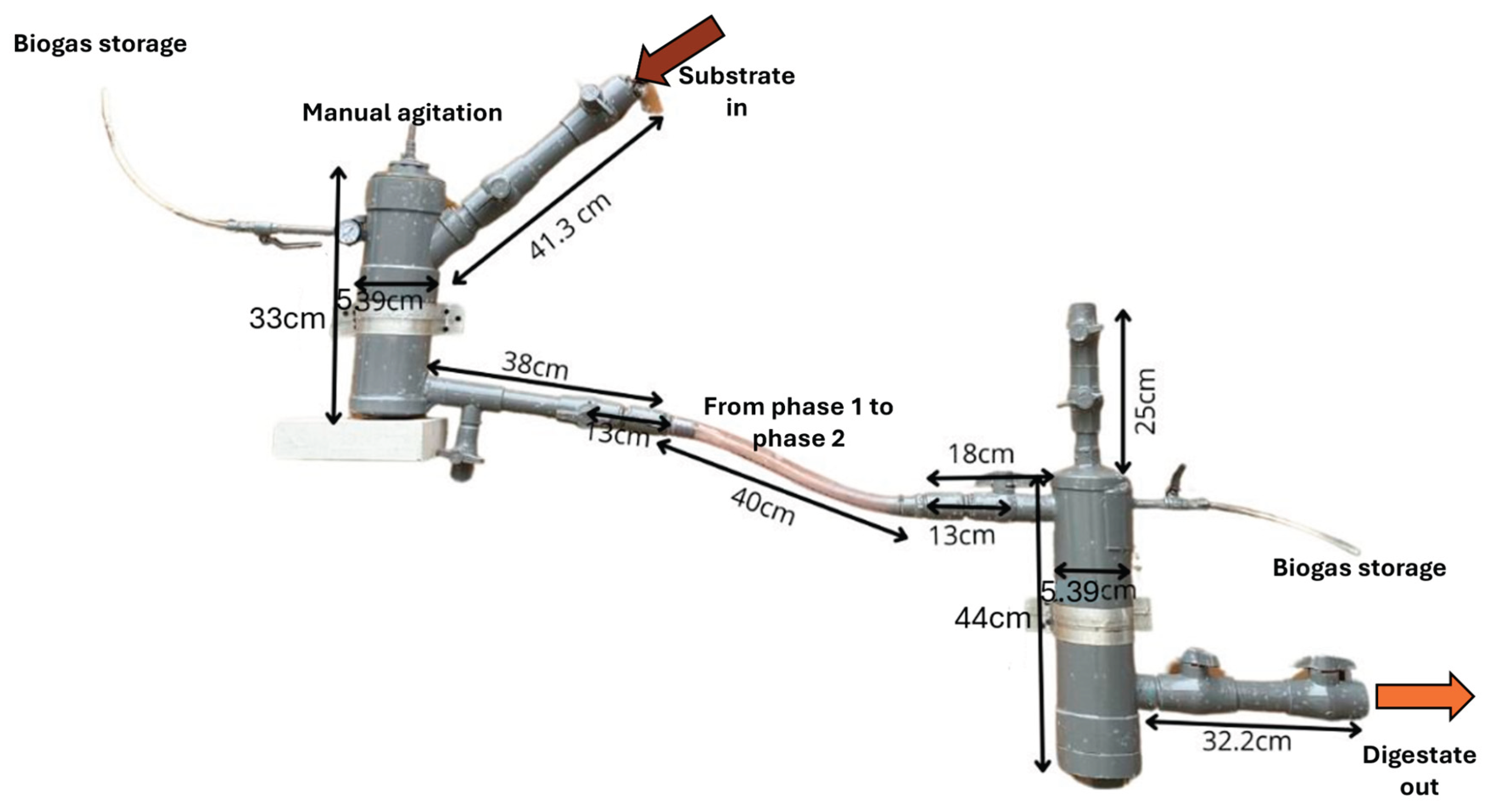
Figure 2.
Original (58 points) vs. interpolated (1000 points) time-series data for CH4 concentration.
Figure 2.
Original (58 points) vs. interpolated (1000 points) time-series data for CH4 concentration.
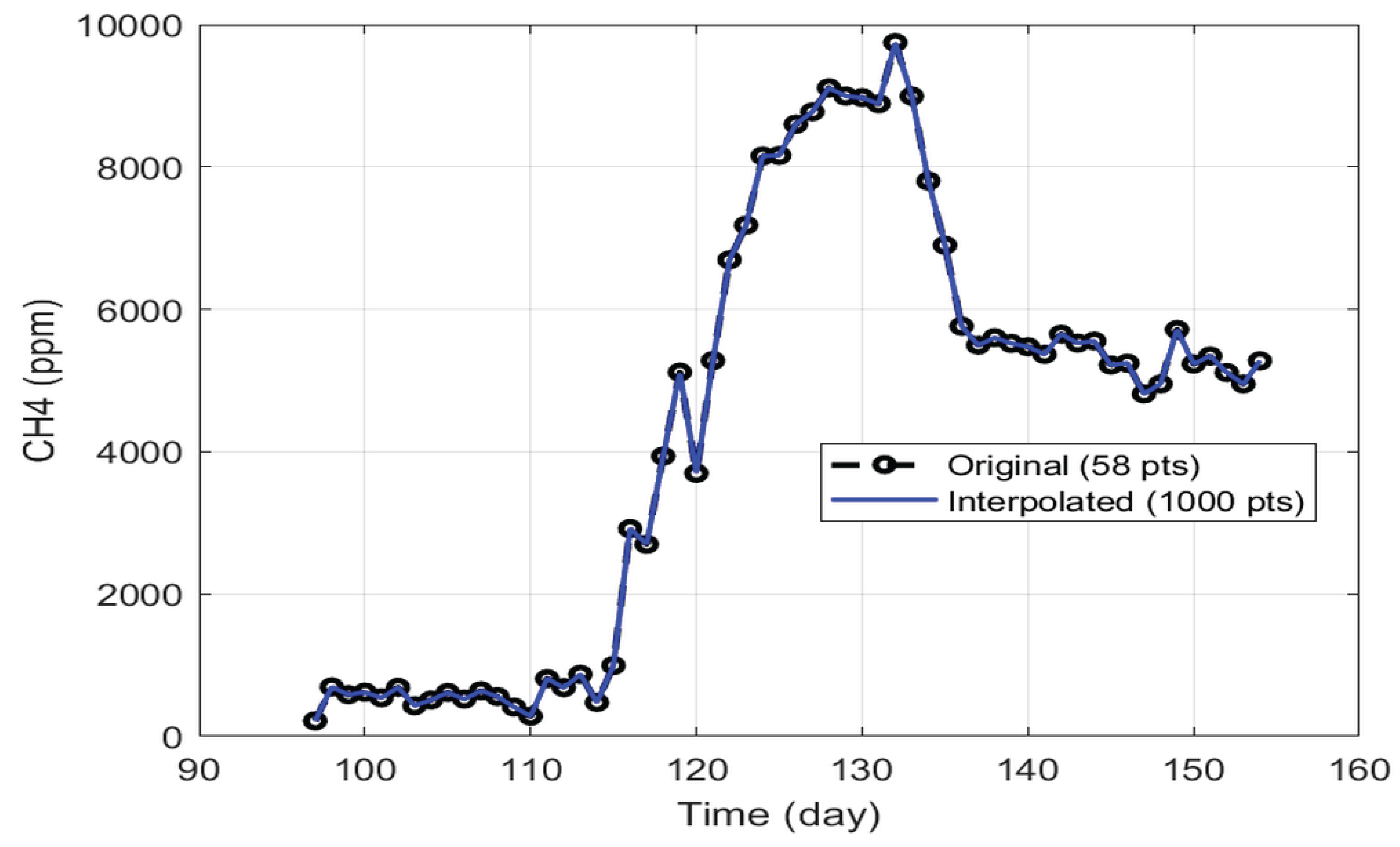
Figure 3.
D1F1 operation during 24 hours on random days.
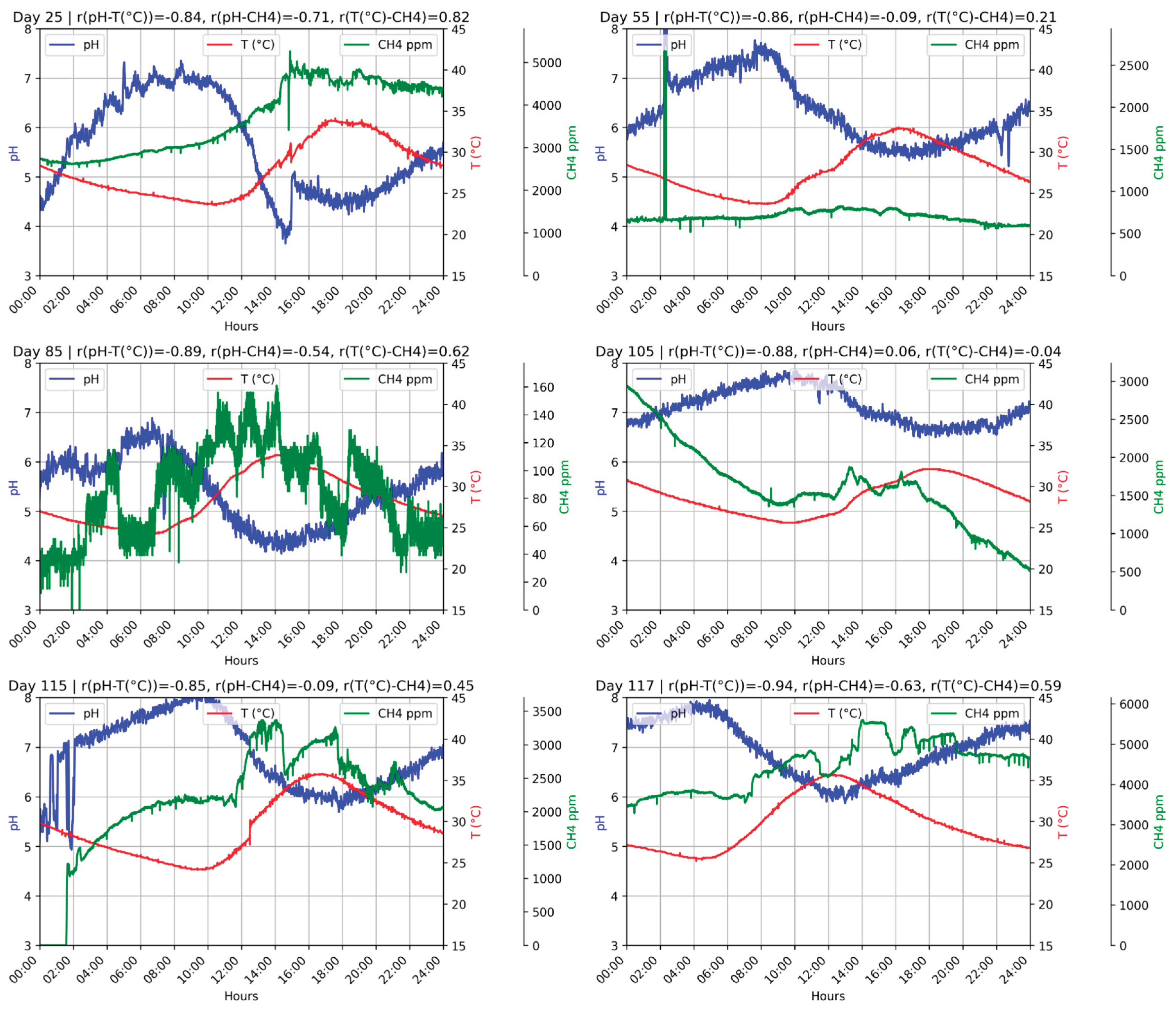
Figure 4.
D1F2 operation during 24 hours on random days.
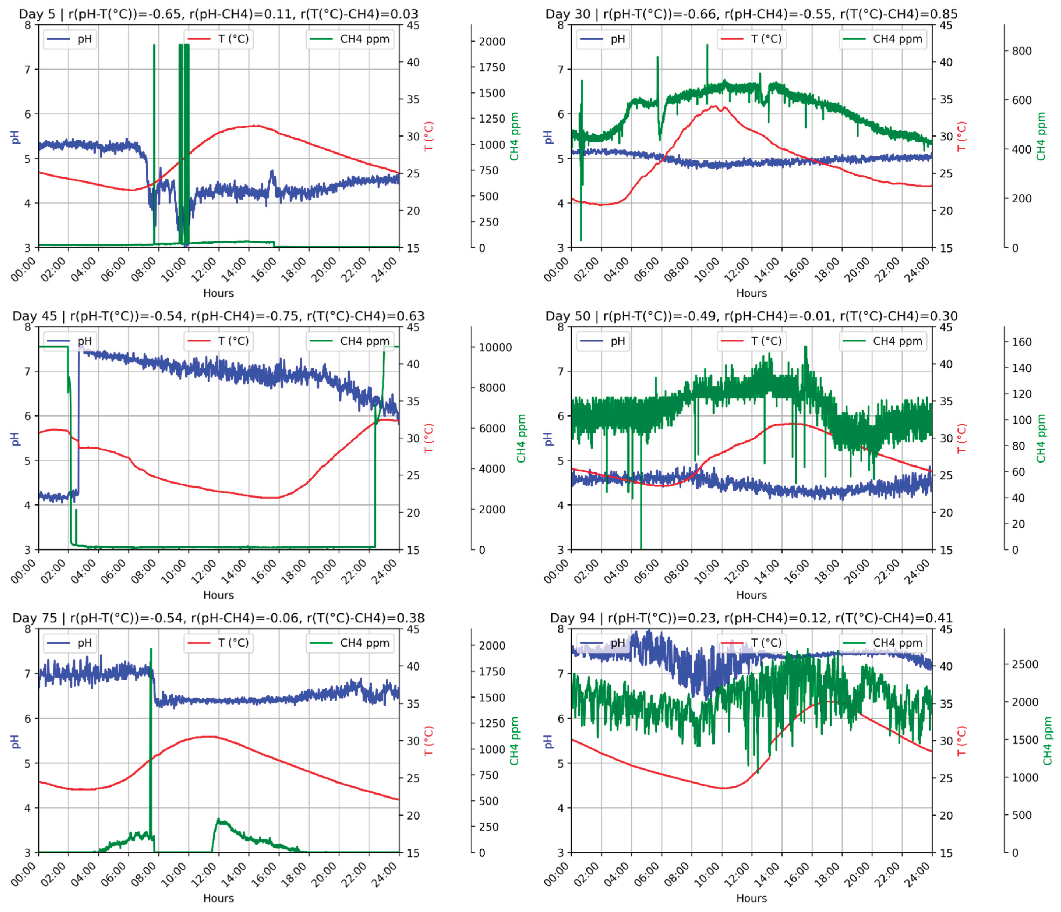
Figure 5.
a) Mixture feeding over time b) Steady-state identification.
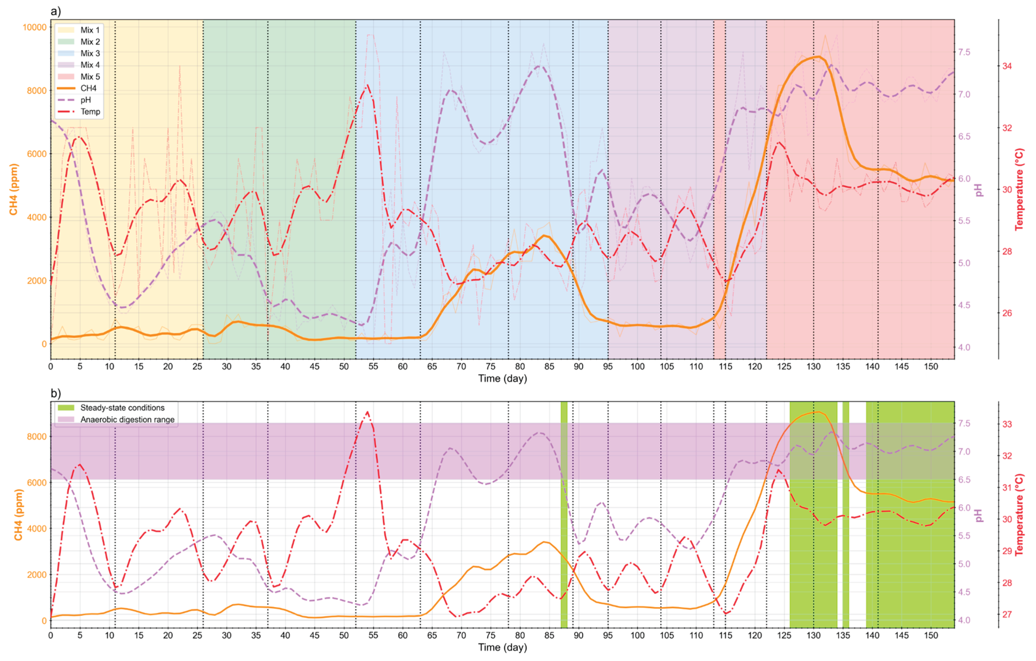
Figure 6.
VFA and alcohol concentration in D1.
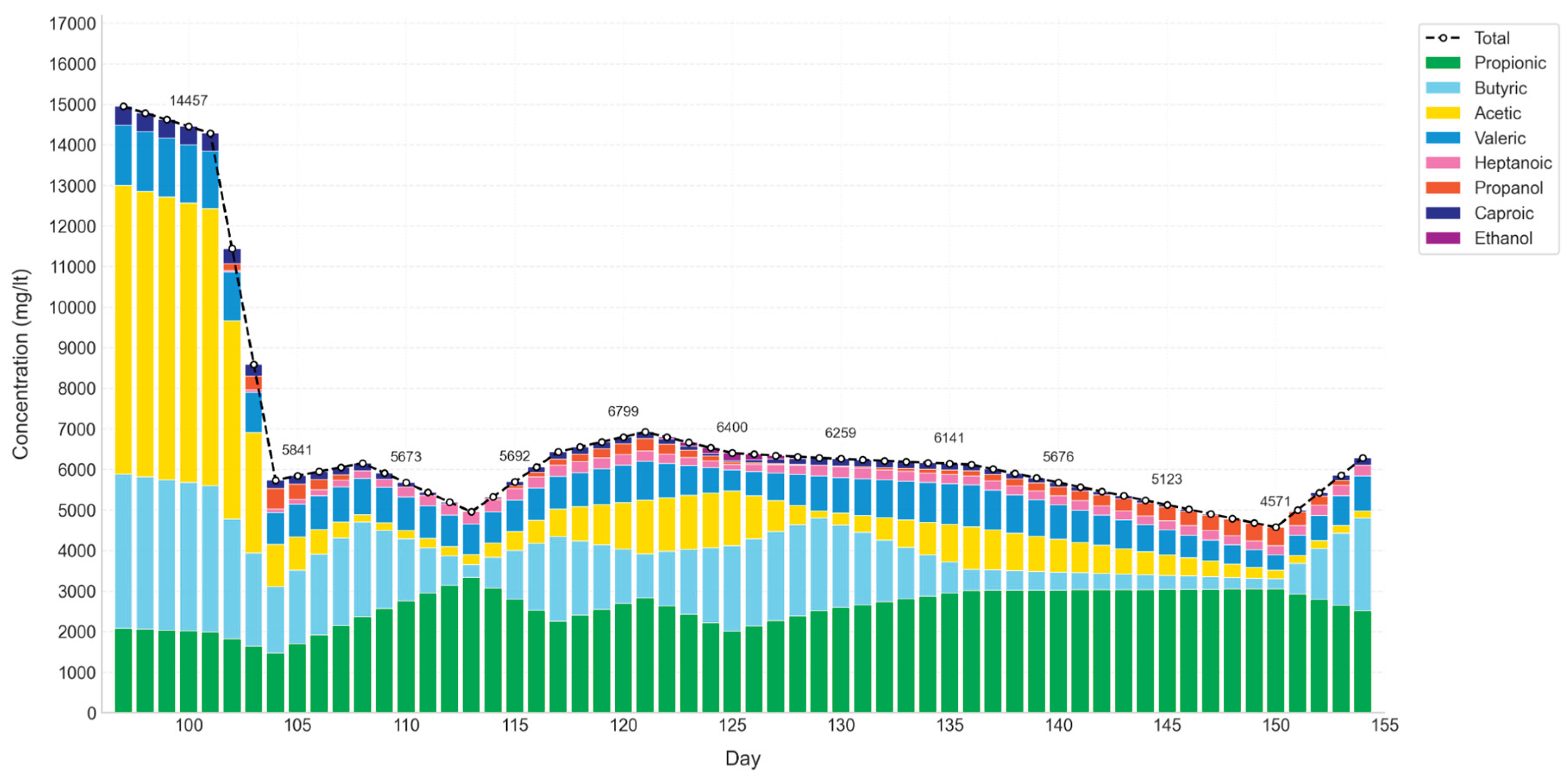
Figure 7.
Alpha rarefaction curves of the alpha diversity (Shannon) of the 16S rRNA gene.
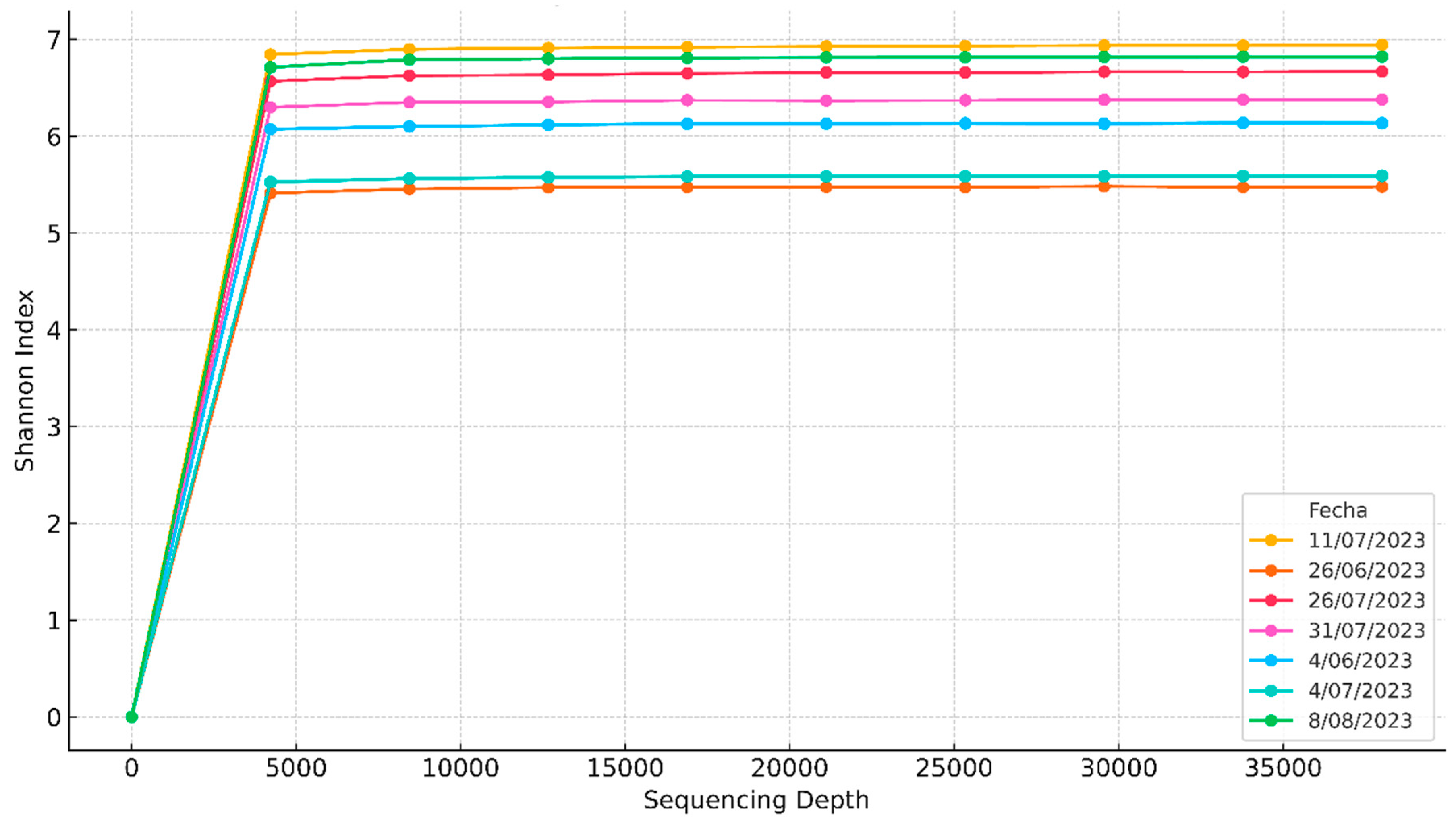
Figure 8.
Temporal dynamics of microbial phyla in D1.
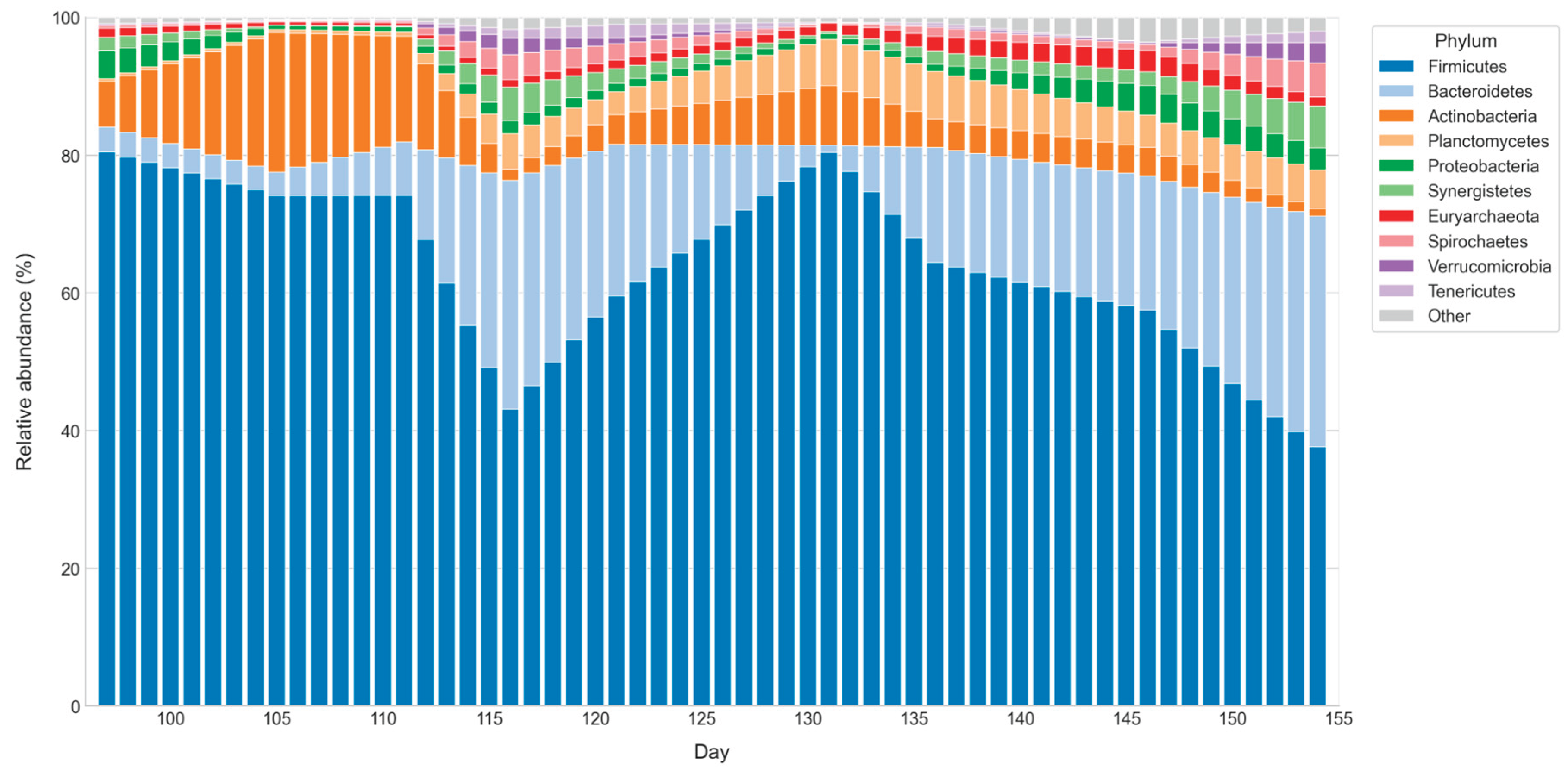
Figure 9.
Approximation result.
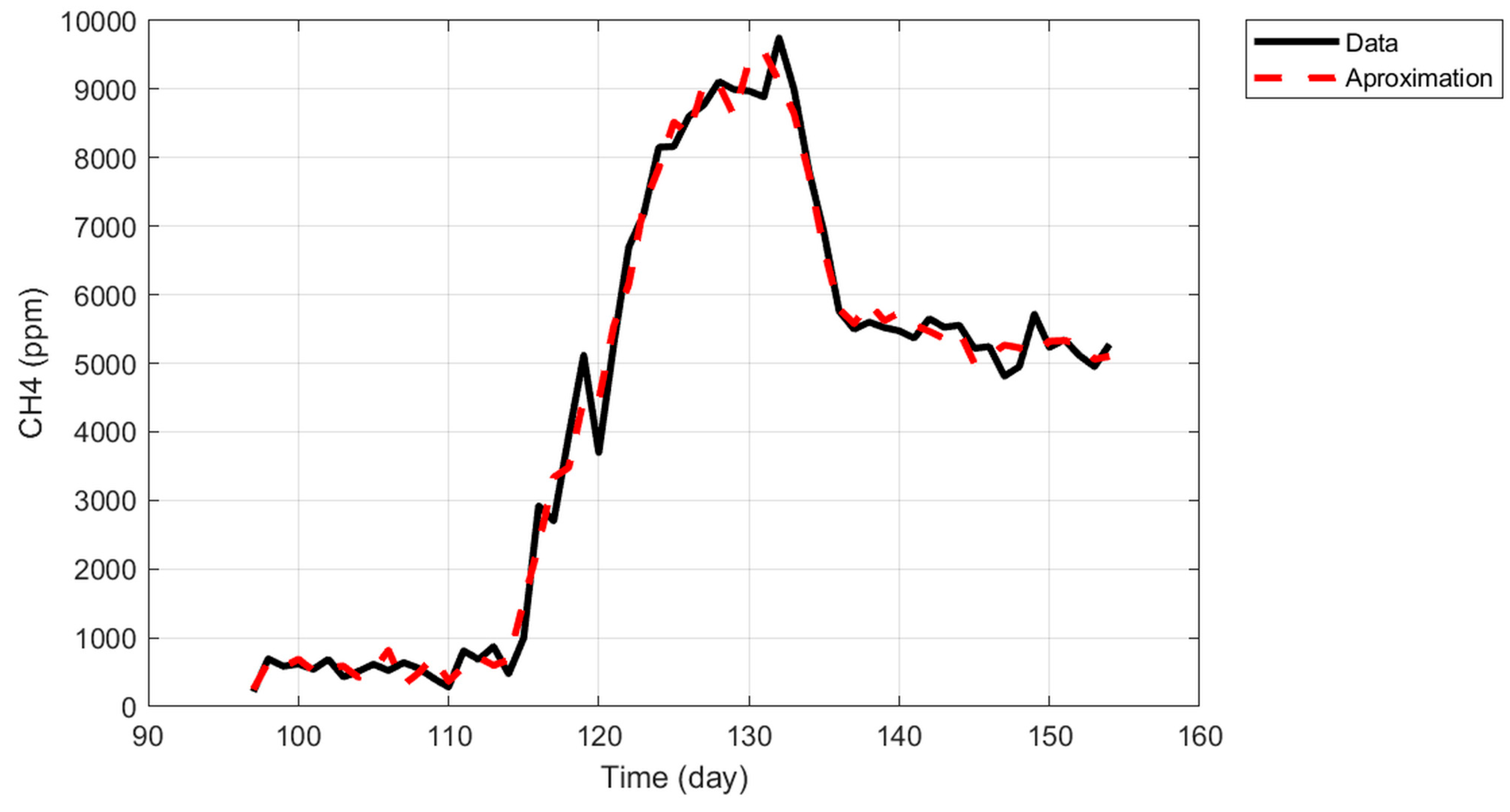
Figure 10.
Relative variable importance with defined cut-off.
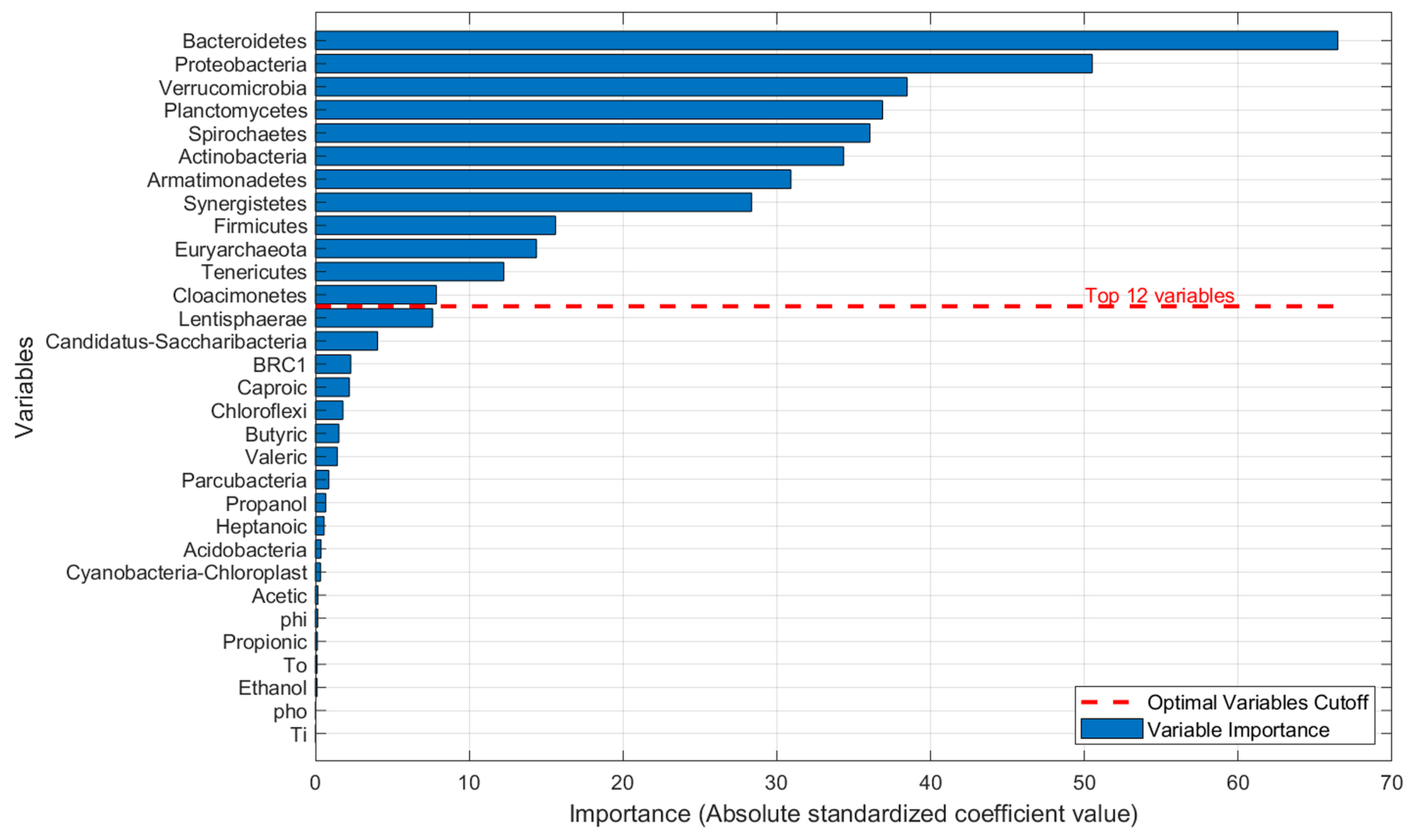
Figure 11.
a) , b) MRE and c) RMSE vs Number of included variables in the approximation.
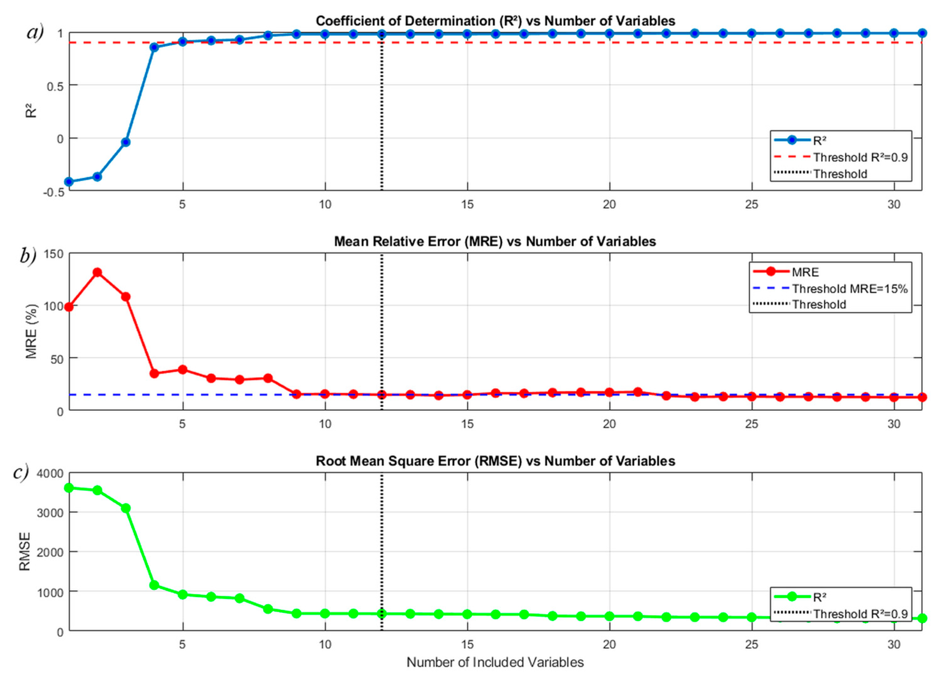
Figure 12.
Weighted approximation.
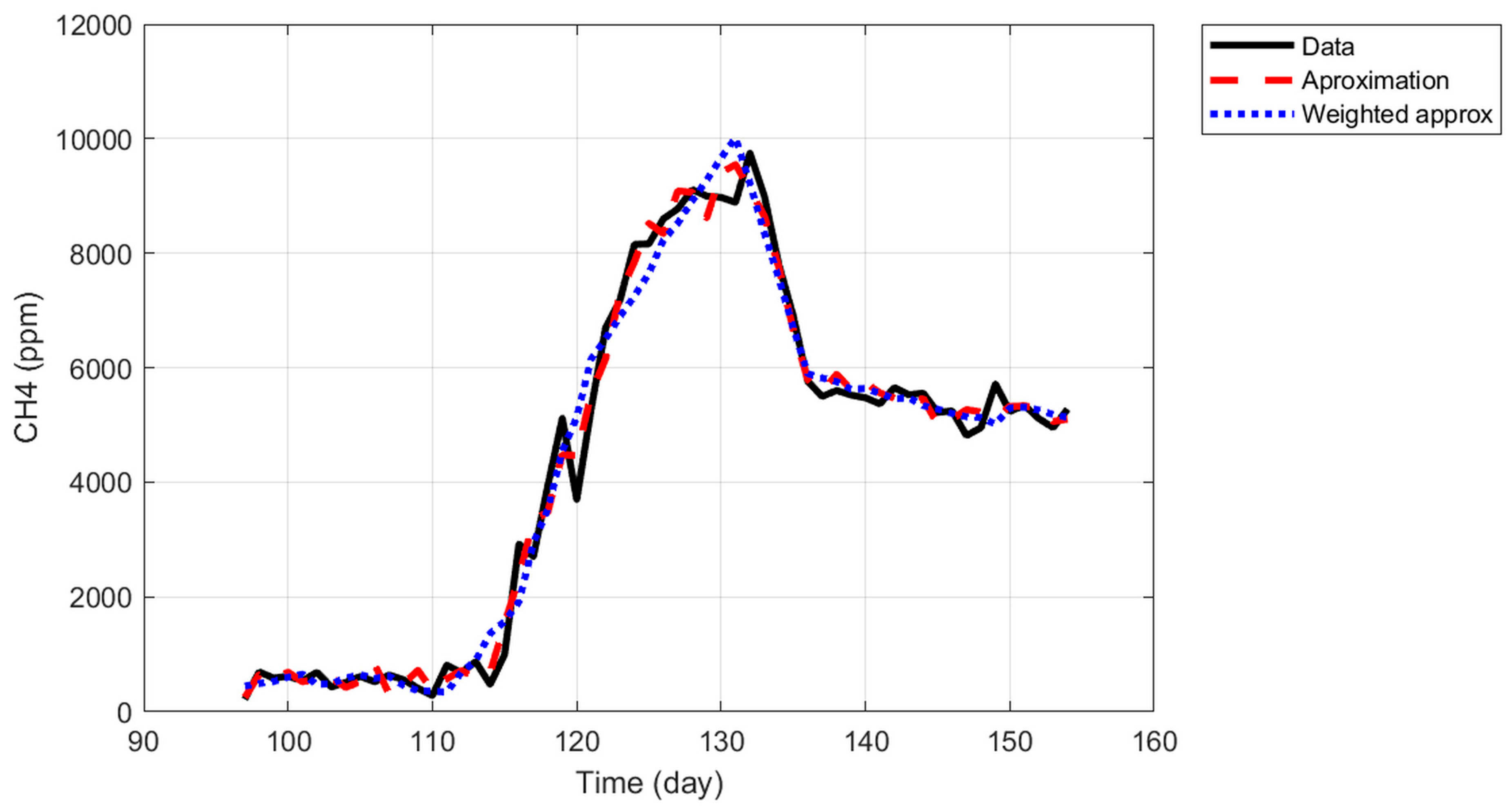
Figure 13.
Behavior of the coefficients associated with the weighted variables.
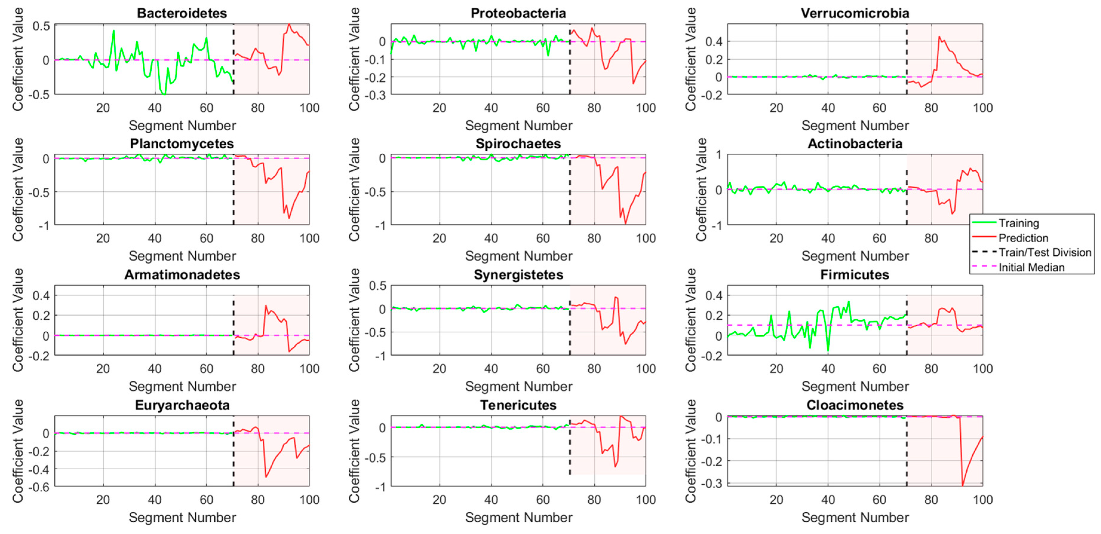
Figure 14.
Methane prediction and training data.
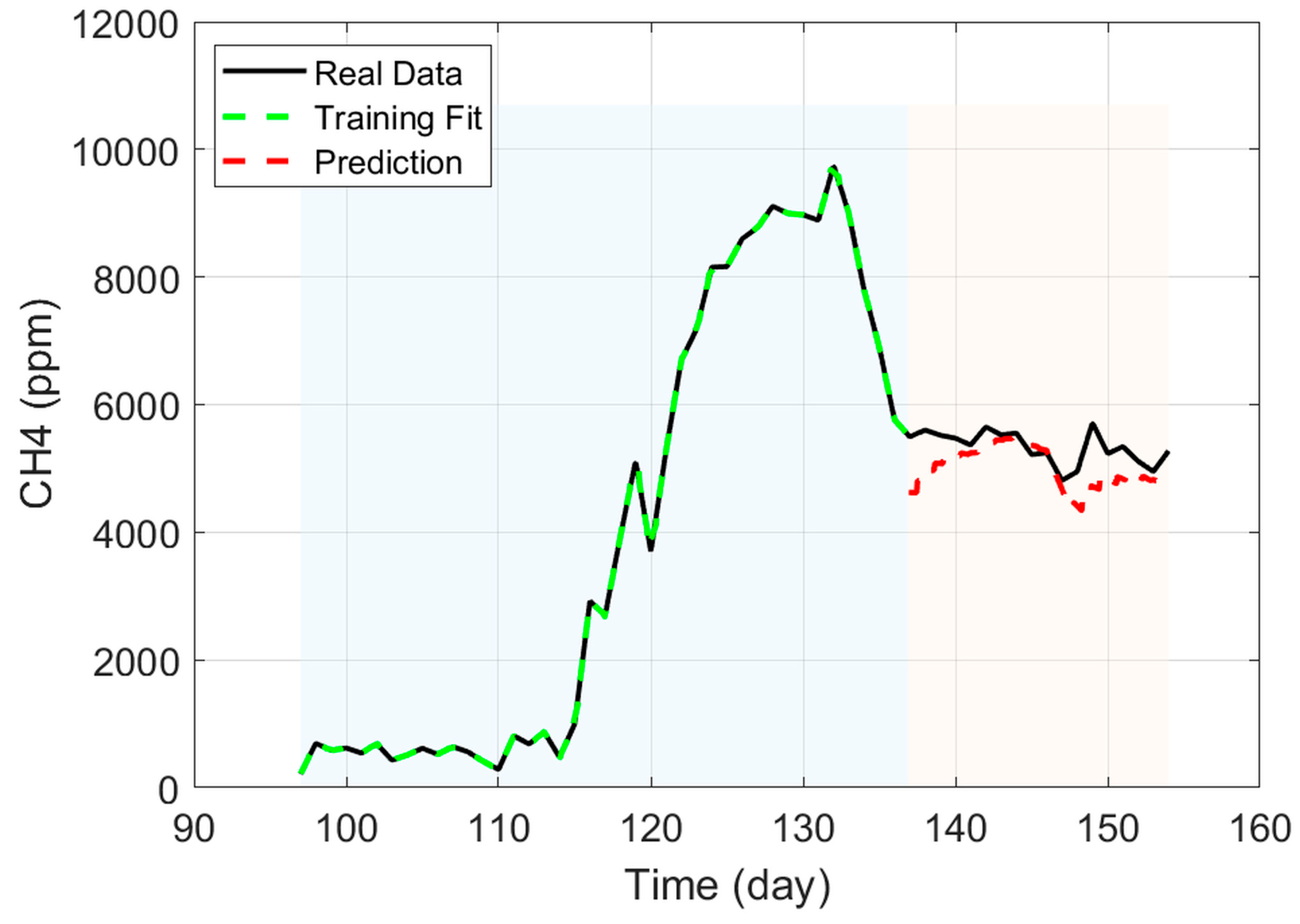

Table 1.
Substrate characerization.
| Substrate | C(%) | N(%) | C:N | %Hum. | %TS | %VS | %VS/%TS | %FS |
|---|---|---|---|---|---|---|---|---|
| I | 32.9 | 3.2 | 10.3 | 98.0% | 2.2% | 1.3% | 60.8% | 0.9% |
| CD | 43.1 | 0.9 | 45.9 | 11.0% | 89.0% | 85.4% | 96.0% | 3.6% |
| PM | 12.9 | 1.9 | 7.0 | 72.0% | 28.0% | 21.0% | 75.0% | 7.0% |
I: Inoculum; CD: Cassava dregs; PM: Pig manure; C: Carbon content: N: nitrogen content.
Table 2.
Adjusted feeding regime.
| D1F1 | |||||||||||||||
|---|---|---|---|---|---|---|---|---|---|---|---|---|---|---|---|
| Mix | OLR (gVS/L·day) | Mix load (g) | I (g) | PM (g) | CD (g) | H2O added (g) | Daily load (g) | %TS | C:N | %I | %PM | %CD | HRT (day) | Period (day) | pH treatment |
| I | 12.40 | 329 | 329 | 152 | 481 | 10% | 10.3 | 100% | 0% | 0% | 5 | 0-.5 | |||
| 1 | 7.67 | 48 | 35 | 13 | 166 | 214 | 10% | 21.6 | 0% | 73% | 27% | 11 | 6-27 | Lime | |
| 2 | 7.66 | 54 | 43 | 11 | 164 | 218 | 10% | 18.3 | 0% | 80% | 20% | 11 | 28-49 | ||
| 3 | 6.60 | 48 | 39 | 9 | 162 | 210 | 9% | 17.5 | 0% | 81% | 19% | 11 | 50-89 | NaOH | |
| 4 | 5.90 | 46 | 14 | 25 | 7 | 165 | 211 | 8% | 15.7 | 30% | 54% | 15% | 11 | 90-118 | NaOH |
| 5 | 5.87 | 71 | 35 | 26 | 10 | 136 | 207 | 8% | 20.7 | 50% | 36% | 14% | 11 | 119-161 | |
| D1F2 | |||||||||||||||
| I | 12.40 | 439 | 439 | 202 | 641 | 10% | 10.3 | 100% | 0% | 0% | 5 | 0-.5 | |||
| 1 | 5.75 | 48 | 35 | 13 | 166 | 214 | 10% | 21.6 | 0% | 73% | 27% | 15 | 6-38 | ||
| 2 | 5.74 | 54 | 43 | 11 | 164 | 218 | 10% | 18.3 | 0% | 80% | 20% | 15 | 39-60 | ||
| 3 | 4.95 | 48 | 39 | 9 | 162 | 210 | 9% | 17.5 | 0% | 81% | 19% | 15 | 61-100 | ||
| 4 | 4.41 | 46 | 14 | 25 | 7 | 165 | 211 | 8% | 15.7 | 30% | 54% | 15% | 15 | 101-127 | |
| 5 | 4.40 | 71 | 35 | 26 | 10 | 136 | 207 | 8% | 20.7 | 50% | 36% | 14% | 15 | 128-161 | |
I = inoculum; PM = pig manure; CD = cassava dreg; OLR = organic loading rate; TS = total solids; HRT = hydraulic retention time.
Table 3.
Data processing.
| D1F1 | |||||
|---|---|---|---|---|---|
| Steps | pH | T(°C) | CH4 | Total | % |
| All data | 694110 | 694110 | 694110 | 2082330 | 100% |
| Day-hour | 694110 | 694110 | 694110 | 2082330 | 100% |
| Filters | 635953 | 635953 | 635953 | 1907859 | 92% |
| MICE | 694110 | 694110 | 694110 | 2082330 | 100% |
| Data per hour | 2893 | 2893 | 2893 | 8679 | 0.42% |
| Data per day | 152 | 152 | 152 | 456 | 0.02% |
| D1F2 | |||||
| All data | 573215 | 573215 | 573215 | 1719645 | 100% |
| Day-hour | 573215 | 573215 | 573215 | 1719645 | 100% |
| Filters | 518897 | 518897 | 518897 | 1556691 | 91% |
| MICE | 573215 | 573215 | 573215 | 1719645 | 100% |
| Data per hour | 2389 | 2389 | 2389 | 7167 | 0.42% |
| Data per day | 147 | 147 | 147 | 441 | 0.03% |
Table 4.
List of associated suffixes for fatty acids (a).
| Acetic | 1 | Caproic | 5 | |
| Propionic | 2 | Heptanoic | 6 | |
| Butyric | 3 | Ethanol | 7 | |
| Valeric | 4 | Propanol | 8 |
Table 5.
List of associated suffixes for microorganisms (m).
| Firmicutes | 9 | Tenericutes | 19 | |
| Bacteroidetes | 10 | Armatimonadetes | 20 | |
| Actinobacteria | 11 | Cyanobacteria Chloroplast | 21 | |
| Proteobacteria | 12 | Acidobacteria | 22 | |
| Planctomycetes | 13 | Lentisphaerae | 23 | |
| Synergistetes | 14 | BRC1 | 24 | |
| Spirochaetes | 15 | Candidatus Saccharibacteria | 25 | |
| Euryarchaeota | 16 | Parcubacteria | 26 | |
| Verrucomicrobia | 17 | Chloroflexi | 27 | |
| Cloacimonetes | 18 |
Table 6.
List of associated suffixes for operating conditions (p).
| phi | 28 | pho | 30 | |
| Ti | 29 | To | 31 |
Table 7.
Approximation coefficients.
| -0.25 | 84.58 | ||
| 0.72 | 152.94 | ||
| 4.86 | -154.01 | ||
| 18.20 | -112.07 | ||
| -61.33 | 165.65 | ||
| -22.60 | 60.94 | ||
| -12.08 | 15.47 | ||
| 14.33 | -302.56 | ||
| 7.39 | 159.10 | ||
| -18.99 | -450.57 | ||
| -21.21 | 81.69 | ||
| -161.69 | 116.88 | ||
| -58.79 | -1562.95 | ||
| 67.72 | 6.72 | ||
| 123.17 | 68.50 | ||
| 242.54 |
Table 8.
Weighting parameters
| 66.48 | 2.21 | ||
| 50.51 | 1.79 | ||
| 38.48 | 1.53 | ||
| 36.87 | 1.43 | ||
| 36.06 | 0.88 | ||
| 34.35 | 0.67 | ||
| 30.92 | 0.57 | ||
| 28.37 | 0.37 | ||
| 15.61 | 0.34 | ||
| 14.37 | 0.17 | ||
| 12.25 | 0.15 | ||
| 7.87 | 0.13 | ||
| 7.63 | 0.11 | ||
| 4.04 | 0.11 | ||
| 2.30 | 0.01 | ||
| 0.01 |
Table 9.
New weighted approximation coefficients.
| -4.64 | 63.94 | ||
| -42.40 | 16.20 | ||
| -94.76 | 1.70 | ||
| -7.66 | -7.10 | ||
| 64.88 | -22.13 | ||
| -4.02 | 251.39 |
Table 10.
Precision metrics for approximations and real data.
| [ppm] | |||
|---|---|---|---|
| All variables | 0.989 | 12.59 | 319.94 |
| Weighted aproximation | 0.979 | 14.94 | 435.82 |
Table 11.
Evaluation of the training model and predictive model.
| Training Fit | 0.999 | 0.35 | 20.77 |
| Prediction | 0.920 | 6.50 | 139.84 |
Disclaimer/Publisher’s Note: The statements, opinions and data contained in all publications are solely those of the individual author(s) and contributor(s) and not of MDPI and/or the editor(s). MDPI and/or the editor(s) disclaim responsibility for any injury to people or property resulting from any ideas, methods, instructions or products referred to in the content. |
© 2025 by the authors. Licensee MDPI, Basel, Switzerland. This article is an open access article distributed under the terms and conditions of the Creative Commons Attribution (CC BY) license (http://creativecommons.org/licenses/by/4.0/).
Copyright: This open access article is published under a Creative Commons CC BY 4.0 license, which permit the free download, distribution, and reuse, provided that the author and preprint are cited in any reuse.


