Submitted:
26 August 2025
Posted:
27 August 2025
You are already at the latest version
Abstract
Introduction: The S&P consists of eleven business segments, which are classified according to the type of industry. The current study focuses on developing a non-linear analytical model for the Healthcare Business Segment (HBS) of the S&P 500, as a function of different economic & financial indicators. Materials and Methods: The analytical model used six financial indicators together with four economic indicators to predict the weekly average closing price (WCP) of HBS stocks. Johnson’s SB transformation corrected skewness, while desirability-based optimization identified indicator values maximizing WCP. The model’s performance and generalizability were validated through repeated 10-fold cross-validation. Results: All attributable contributors were ranked in accordance with the percentage of contribution to the WCP. The cross-validated R2s and RMSEs were found to be consistent across each fold for the proposed analytical model. The R2 (96.74%) and adjusted R2 (96.03%) were found to be high and consistent for the test (unseen) dataset. Discussions: The analytical modeling produces vital information that helps investors and portfolio managers, and financial institutions evaluate healthcare industry investments in the S&P 500. The optimization strategy helps identify the best controllable factors, which leads to more precise and strategic decision-making Patents: This paper has also been submitted for a US provisional patent on 31 May 2023 (TTO ref. 23T220PR-CS).
Keywords:
healthcare business segment (HBS)
; financial & economic indicators
; analytical optimization
; desirability function
; nonlinear statistical model
1. Introduction
Stock price forecasting stands as a fundamental subject in finance because precise predictions deliver essential information to investors and policymakers and researchers. The Efficient Market Hypothesis (EMH) within traditional financial theory states that stock prices contain all available information thus making systematic prediction challenging. Empirical research has proven that both financial indicators from individual firms and macroeconomic variables explain stock return variations thus contradicting the EMH. Predictive modeling of financial markets now focuses increasingly on combining micro-level firm fundamentals with macro-level economic conditions.
The initial research in this field demonstrated that financial ratios at the firm level play a crucial role. Fama and French (1992) established through their research that size and value-related factors including book-to-market ratios explain enduring patterns in expected returns which demonstrates the predictive strength of company fundamentals [1]. Piotroski (2000) created the F-score to show that financial health composite measures can identify firms which will perform better in the future thus validating accounting-based prediction methods [2]. Stock price behavior shows consistent links with firm-specific measures including dividend yield and earnings capacity and free cash flow which indicates that forecasting models depend heavily on fundamental company data.
Research has shown that macroeconomic factors play a crucial role in the same way as the findings mentioned above. Chen, Roll, and Ross (1986) were among the first to establish a systematic link between economic forces and stock prices, showing that variables such as inflation, industrial production, and interest rate spreads significantly influence asset valuations [3]. Later work expanded on this framework by incorporating measures such as GDP growth, consumer sentiment, and personal saving rates, thereby capturing the broader economic environment that shapes market valuations ([4,5]). These contributions highlight that stock markets do not evolve in isolation but are deeply embedded in macroeconomic dynamics.
The Standard & Poor 500 (S&P 500) consists of 500 large-cap companies that are selected based on size, liquidity, and industry, which are essential to all investors in the stock market. It is one of the most widely used benchmarks for measuring the performance of large-capitalization, U.S.-based stocks, which is updated recurrently [6]. Investors meticulously study the S&P 500 to assess the overall behavior of the stock market. Stock prices are the most distinguishable of all financial measures that can be used to evaluate the performance of several companies.
The S&P 500 index is prominently recognized as a benchmark for the broader US equities market and has been the subject of extensive study by investors and researchers ([7,8]). Within this influential index, the healthcare sector has emerged as an area of significant interest. This industry encompasses a diverse array of companies engaged in the production and distribution of medical goods, the delivery of healthcare services, and the development of pharmaceutical and biotechnology innovations. By analyzing the performance of the healthcare sector within the broader S&P 500 framework, researchers can uncover valuable insights into the factors driving overall market behavior and the role of the healthcare industry in shaping broader economic trends.
Healthcare is a major requirement for everyone, or at least almost everyone needs it at some point in their lives, and when there is something that everybody requires, there’s a massive opportunity for investors. More than 7.8 trillion is spent on healthcare globally. Approximately half of that total, 3.5 trillion, is spent in the U.S. From 1996 to 2016, total healthcare spending increased from an estimated $ 1.4 trillion to an estimated $ 3.1 trillion [9]. Because the healthcare sector is developing at a higher rate than the global economy, these figures will presumably be considerable by the end of the decade. Exploring the relationship of different stocks within the HBS of the S&P 500 is crucial to grasp the broader trends and dynamics in the US stock market. Chen et al. explored the dynamic relationship of returns in the health sector among different stock markets using continuous wavelet analysis. Their findings revealed that, among the three health care systems studied (the US, UK, and Germany), the UK and US represent two extremes, as reflected in the distinct patterns of their wavelet power spectra. This suggests that the structure of a country’s health care system may influence the return dynamics of its health sector [10].
The healthcare sector is crucial to the overall economy, so its performance can significantly impact the broader market, and vice versa. Predicting stock prices, particularly for sectors like healthcare within the S&P 500, presents a significant challenge for investors and financial analysts ([11]). This difficulty stems from the complex and dynamic nature of financial markets, characterized by non-stationary behaviors and sensitivity to various economic and financial indicators ([12]). While the efficient market hypothesis suggests that consistently outperforming the market through prediction is not possible, research indicates that carefully constructed and optimized predictive models can achieve meaningful accuracy ([13]). These models often integrate technical analysis, which uses historical price and volume data, with fundamental analysis, which assesses a company’s financial health and broader economic conditions ([14]). The healthcare sector, with its unique sensitivity to regulatory changes, demographic shifts, and technological advancements, offers a compelling case study for predictive modeling ([15]).
Previous studies have explored the intricacies of the US healthcare system, examining the relationship between economic growth and healthcare expenditures [16,17]. While there is a wealth of literature on the US healthcare landscape, limited research has comprehensively analyzed the connections between economic indicators and healthcare system metrics, as well as strategies for reforming this vital sector. Stock price maximization [18] is one of the most significant attributes for value maximization objectives. One of the main goals of this study is to optimize the developed analytical model that predicts the weekly closing price (WCP) of the healthcare business segment (HBS) of the S&P 500 as a function of financial & economic indicators. Many researchers and business analysts strongly believe that dividend yield plays a crucial role in stock returns. Higher stock returns are now well known to be related to larger dividends, regardless of whether income is taxed more or less highly than capital gains [19]. One of the most crucial indicators to influence the return is the price-to-earnings ratio (P/E ratio). Studies [20] have found a direct relationship between price to price-to-earnings ratio with the stock return, and the returns were changed more by the P/E ratio than the price/earnings-to-growth (PEG) ratio, and thus, stock returns of firms are more affected by the P/E ratio than the PEG ratio. Tang and Shum [21] have found a significant relationship between the ups and downs of individual stock and the beta risk. The Piotroski Score/F Score is another economically meaningful and statistically significant predictor of the cross-section of international stock returns, which was developed by Chicago accounting professor Joseph Piotroski, who devised a scale according to some specific aspects of a company’s financial statements [22]. The Piotroski score [2] is a discrete numerical score between 0 to 9 that reflects nine criteria used to decide the strength of a firm’s financial stability. The score is utilized to determine the best value stocks, with nine being the best and zero being the worst. [23] found that the portfolios formed from companies that rank high on their F-Scores show higher risk-adjusted returns than portfolios of low F-Scores by utilizing data from the Finnish stock market. [24] found similar results using the Warsaw Stock Exchange data from 2014 to 2020. Earnings Before Interest, Taxes, Depreciation, and Amortization (EBITDA) is a measure of a company’s overall financial performance. EBITDA is the performance measure for valuation, debt contracting, and executive compensation and was found to perform substantially better in comparison with both EBITA and EBIT [25,26]. The free cash flow (FCF) is important in determining a company’s cash flow after deducting the purchase of assets such as property, equipment, and other major investments from its operating cash flow. Free cash flow is a pivotal metric since it describes how dynamic a company is at generating cash, which is utilized by the investors to measure if a company might have sufficient cash, after all the capital expenditures [27]. Numerous empirical and case studies have shown to have a strong relationship between the macroeconomic variables and the stock prices [28,29,30,31,32,33]. Lemmon and Portniaguina [34] have shown that a consumer’s confidence exhibits forecasting power for the stock return. The Index of Consumer Sentiment (ICS), or economic well-being, was developed at the University of Michigan Survey Research Center to measure the confidence or optimism (pessimism) of consumers in their future well-being and upcoming economic conditions. The index measures short and long-term expectations of business conditions and the individual’s perceived economic well-being. Evidence [35] indicates that the ICS is a leading indicator of economic activity, as consumer confidence seems to pave the way for major spending decisions. [36] shows how consumer sentiment affects consumption expenditures and stock returns in the hospitality industry. The author suggests that the predictive ability of consumer sentiment can be useful to managers in business forecasting, planning, and strategizing for profit maximization, since changes in consumer sentiment partly predict changes in the stock prices of hospitality firms. The US inflation rate is another major metric used by the US Federal Reserve to estimate the health of the economy and globalization [37]. Significant dynamic conditional correlations were found between stock price and inflation in the United States [38]. Albulescu et al. found that, contrary to the well-known Fisher effect, inflation and its uncertainty negatively affect stock prices in the long run. However, for several sector stock indexes, this negative impact disappears following the crisis outburst [39].
The U.S. Personal Saving Rate (PSR) is the personal savings as a percentage of disposable personal income [40]. In other words, it’s the percentage of people’s incomes left after they pay the essential expenses. Personal saving habits have a significant impact on an individual’s financial health, as the lack of financial literacy is a significant deterrent to stock ownership and accumulation of wealth [41]. In structuring the analytical model, the average weekly closing price (WCP) for the 59 healthcare stocks was considered as the dependent variable (response); thus, the analytical model consists of the significant contributable variables (indicators) and significant two-way interactions between the indicators. The validation and quality of our proposed analytical model have been statistically evaluated using R-squared (), R-squared adjusted (), root mean square error (), and ten-fold repeated cross-validation. To the best of our knowledge, no such statistical model has been constructed to predict the WCP of the healthcare business segment (HBS) of S&P 500 using the proposed logical framework, along with the optimization strategy, by identifying the optimum levels of the indicators, with at-least 95% confidence. Therefore, developing an appropriate analytical model for the HBS of S&P 500 is relevant in the context of economics & financial literature. The development of the current manuscript is as follows: In Section 2, we discuss the development of the analytical model that predicts the weekly closing price (WCP) as a function of the indicators. Section 2.1 and Section 2.2 talk about the model diagnostics, and model validation, followed by the analytical method of optimization of the WCP of the HBS in Section 3. Under Section 4, we present the discussion along with the graphical representations of the optimization results, followed by the concluding remark in Section 5.
2. Materials and Methods
The indicators that have been included in our model have significant relevance in the literature of finance. We have included six financial indicators (the dividend yield (), the beta risk (), the price-to-earnings (PE) ratio (), the Piotroski F score (), earnings before interest, taxes, depreciation, and amortization (), and free cash flow ()) and four economic indicators (the US GDP (), the Index of US Consumer Sentiment (), the US personal saving rate (), and the US inflation rate ()) in our proposed analytical model, along with the significant two-way interactions. Prior to developing the analytical model for the WCP of the HBS as a function of the different indicators, we initially check if the response WCP follows a Gaussian probability distribution. From the following Q-Q plot in Figure 1, we see that the values of the response WCP are positively skewed and do not entirely follow a Gaussian probability distribution.
We have also shown through goodness-of-fit (GOF) testing [42,43] (Shapiro-Wilk normality test, a p-value = ) that the analytical form that drives the WCP does not support the normal probability distribution. In developing the analytical model, the first objective was to express the response variable WCP in terms of a non-linear mathematical function of all indicators. The general analytical form of a model, including all possible indicators (: single indicators (main effects), ) and interactions (: two-way interaction terms, where ) can be expressed by:
where is the intercept of the model, s are the response; s are the coefficients (weights) of the main effect of the predictor , s are the coefficients for the interaction between predictors and , and denotes the random disturbance or residual error of the model. As illustrated earlier, the dependent variable WCP does not support the Gaussian probability distribution; hence, a non-linear transformation was applied to the response variable to determine if the transformation can be suitable to adjust the skewed data. After implementing various non-linear transformations to the data, Johnson transformation [44,45,46] was found to be the most suitable transformation to address the skewed data problem which is described as follows:
where is the scale parameter. is the 1st shape parameter. is the 2nd shape parameter. is the location parameter. z is the transformed response.
After plugging in the estimated values of the parameters, we have the transformed response as follows:
In the above Equation (3), TWCP represents the new response variable (transformed) after Johnson’s Transformation was applied. The transformed data were tested and found to follow the Gaussian probability distribution. Thus, we proceed to estimate the coefficients (weights) of the actual indicators for the transformed data. To develop the analytical model, we initially began with the full statistical model, which included all ten indicators with two-way interaction terms. Thus, at first, we started structuring the model with potential interaction terms and ten indicators. To determine the most significant contributions of both the individual indicators and interactions by eliminating the less important indicators and interactions gradually, the backward elimination method [47,48] was used that is deemed one of the best traditional methods for a small set of feature vectors to address the problem of over-fitting and performing feature selection. To obtain better accuracy, the log transformation of the indicator PE (X3) was used in the model to reduce its high variability. The statistical analysis indicated that all ten indicators significantly contributed to the response. While testing the forty-five possible interactions, thirty-one were found to significantly contribute to the response. The analytical model with significant indicators and interactions for predicting the response is given as:
The TWCP estimate was obtained from Equation 4 above and was based on the Johnson transformation [45,46] of the data; thus, the anti-transformation was implemented to estimate the desired, predicted values of the average weekly stock price (WCP) as follows:
The proposed analytical model will help social researchers, economists, and financial analysts to understand how the weekly stock price varies when any one of the ten indicators is varied, keeping the other indicators fixed. Similarly, with significant interactions. Most commonly, it will estimate the predicted estimates of the response of WCP given the indicators fixed at a specified level. For example, given, , we obtain the predicted response value as 97.03 (from Equation 5). So, given all the values of the indicators, fixed at a particular level, the weekly average stock price for all healthcare stocks is $97.03. Table 1 illustrates the ranking of the indicators and the interactions that contribute to the response, WCP according to their percentage of contribution from model (4).
The ranking of the indicators that drive the WCP of the HBS is important to the investor. That is, monitoring the behavior of the indicators with respect to current existing data can predict the direction of WCP. Also, the individual healthcare companies that constitute the HBS can utilize the information to increase their company’s stock value by concentrating on improving the indicators that contribute most to the WCP. Based on the number of occurrences of each of the ten indicators and their interactions from model 2, the cumulative percentage contributions have been ranked in Table 2. The total sum of the fourth column of Table 2 is more than 100 since we have considered the repeated terms (for example, while determining the percentage of contribution of , we considered the interaction term and other interaction terms with present in model 2. Also, while determining the percentage of contribution of , we considered the interaction term and other interacting terms with present in model 2. The same mechanism was implemented for other indicators in computing the percentage contributions.
2.1. Model Diagnostics
Once the statistical model has been developed, it is important to check the model assumptions by performing residual analysis. The residual error of the proposed model, that is,
where y and are the observed and predicted WCP, respectively. is the estimated residual error from the linear fit. If the sum of the residuals equals almost zero, it is assumed that the regression function is the “best fit.” Also, this ensures an unbiased estimation of the model coefficients. In our case, the mean residual is , implying that it is almost zero as required, and attests to the quality of the developed model. From Figure 2 below, we see that the studentized residuals follow a normal/symmetric pattern that gives an indication about the model’s unbiasedness (doesn’t favor over- or underestimation).
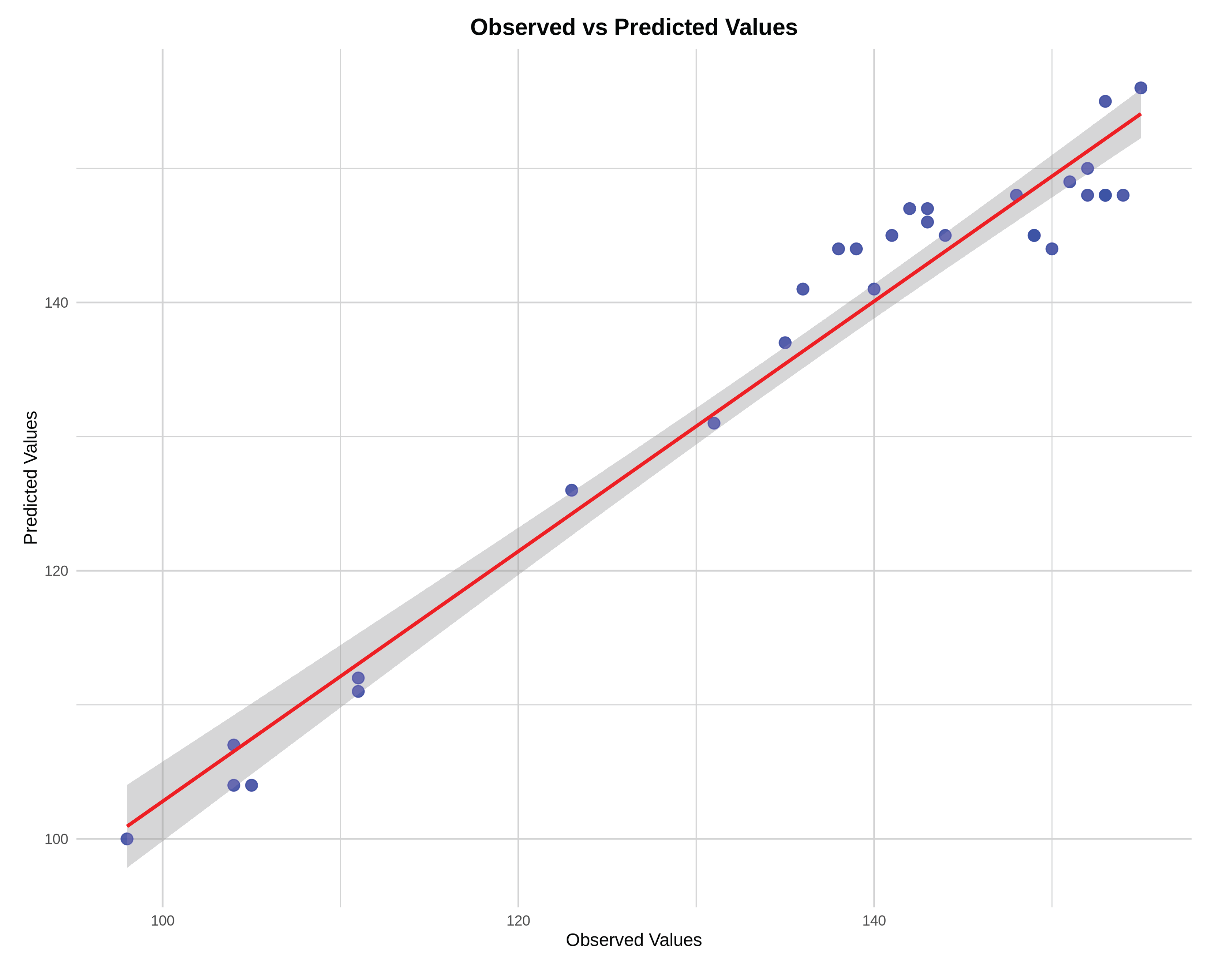
The following figure describes the observed and predicted plot. The plot shows a strong correlation between the observed and the predicted values (correlation coefficient= 0.98, p-value < 0.0001).
Figure 3.
Observed and Predicted Plot.
2.2. Validation of the Proposed Model
To assess the quality of the proposed analytical model, we use both the coefficient of determination, , and adjusted , which are the critical criteria to evaluate the model’s performance [49]. For our final statistical model, the and, adjusted were found to be 96.74%, and 96.03%, respectively. That is, the developed statistical model explains approximately 96.03% of the variation in the WCP as a function of the indicators. The Residual Standard Error (RSE) represents the approximate difference between the observed and predicted outcomes in the proposed model. We obtained an RSE of .21, which implies that the observed response value differs from the predicted response value by .21 on average. The analytical model was developed using training data and was validated on the remaining testing data. In the testing data (validation set), the test error is the average error that occurs from using the analytical model to predict the response to a set of new observations. It addresses the consistency and accuracy of the analytical model. Moreover, we performed repeated ten-fold repeated cross-validation (10 times) [50,51,52,53] for the validation testing. In 10-fold cross-validation, the training set is divided into ten equal subsets. One of the subsets is taken as the testing set in turn, and (10-1) = 9 subsets are taken as a training set in the proposed model. The mean square error is computed for the held-out/validation set. This procedure is repeated 10 times; each time, a different group of observations is treated as a validation set. This process results in 10 estimates of the test error, . The average error of each set throughout the cross-validation process is said to be a cross-validated error. Figure 4 below, illustrates briefly the notion of 10-fold repeated cross-validation, where is the mean square error (MSE) in each iteration and ACVE is the average cross-validated error.
In the validation stage, a high and low attests to the good quality of a model. Also, it is expected that the cross-validated error () and the remain consistent throughout different repeated folds. The following figure illustrates how the and vary in the different folds of the test data.
As Figure 5 illustrates, the is high, and the remains low for different repeated cross-validated folds as expected. Hence, we can conclude that the performance of the proposed model is consistent and robust to new data.
3. Analytical Method to Optimize the WCP of the HBS
Investors, academics, and researchers have all shown an interest in stock market trading and stock price optimization. Numerous algorithms have been created to research market behaviors and improve forecast accuracy in order to analyze the underlying non-linear properties of stock market data, which is an intricate procedure. [54] analyzed the superiority of particle swarm optimization (PSO) for stock portfolio optimization by developing a large number of learning algorithms to study market behaviors and enhance the prediction accuracy of the models. Gülmez devised an AI-based metaheuristics approach (Artificial Rabbits Optimization algorithm (ARO)), an optimized deep LSTM network with the ARO model (LSTM-ARO) to predict stock prices using different evaluation criteria (MSE, MAE, MAPE, and R2) [55].
To forecast stock values for the upcoming period, a hybrid model integrating eXtreme Gradient Boosting (XGBoost) [56,57] and an improved firefly algorithm (IFA) [58] was first presented. In the second stage, stocks with higher potential returns were selected, and the MV model was employed for portfolio selection. Using the Shanghai Stock Exchange as the study sample, the authors found the proposed method to be superior to the traditional ways (without stock prediction) and benchmarks in terms of returns and risks. Once we have developed a high-quality model that identifies the financial and economic indicators and their interactions that predicts the WCP with a high degree of accuracy, we proceed to determine the optimum values of the indicators that will optimize (maximize) the response, WCP. The analytical process is discussed below.
3.1. Analytical Approach Using the Desirability Function
The process of the desirability function for the optimization of the WCP has been used from the proposed analytical model. The desirability function approach was initially proposed by Harrington [59,60], and has been introduced in the literature with respect to Response Surface Methodology (RSM) [61,62]. The desirability function transforms each of the estimated response to a desirability value , where . For an individual response , a desirability function takes on values within [0,1]. , represents entirely an undesirable response and , represents a completely desirable or ideal response. The value of increases as the "desirability" of the corresponding response increases. The individual desirabilities are then merged together using the geometric mean, which gives the overall desirability function, that is,
where k denotes the number of responses. In our model, , the WCP.
Depending on whether a particular response is to be maximized, minimized, or assigned a target value, different desirability functions can be used. A useful class of desirability functions was proposed by Derringer and Suich, [63]. Let , and be the lower, upper, and target values, respectively, that are desired for response , with .
If there is a specific target set up for the response, then its desirability function is given by,
where s and t in the above equation determine how important it is to hit the target. For , the desirability function increases linearly towards the direction of . For , the desirability function is convex, and for , the desirability function is concave [63]. Our objective is to maximize the response, WCP; Thus, the individual desirability function will be,
where and are chosen by the investor. We propose the following five-step algorithm to optimize the response, WCP based on the desirability function method:
- Develop the statistical model that very accurately predicts the response, WCP, driven by a set of significant indicators.
- Obtain the constraints on input indicators, for and ; Y being the response and x being the indicators.
- Define the desirability function(s) for the response(s) based on the optimization objective.
- Obtain the optimal values of the response by maximizing the desirability function with respect to the controllable input indicators.
- Validate the optimization process based on the coefficient of variation and the .
3.2. Numerical Results
The non-linear analytical model is a function of six financial indicators and four economic indicators, along with 31 interactions of the indicators. After developing the predictive model, the next goal was to optimize (maximize) the response WCP to obtain the optimum values of the indicators at which the response was being maximized, utilizing constrained optimization. The analytical method of optimization required the constraints of optimization, as presented in Table 3 for the ten indicators. These constraints were the lower and upper boundaries of each of the ten indicators. In the optimization technique, the optimized response WCP was found to be within its domain, given the specific values of the indicators.
Using Equation (8) of Section 3.1, we can maximize the estimated response from Model (5) and obtain the optimum values of all ten indicators. The following Table 4 provides the estimated maximum response WCP along with the optimum values of the indicators.
Thus, with these values of economic and financial indicators, we are at least 95% certain that the response WCP will be optimized. Furthermore, we can track the numerical behavior of the indicator to determine the direction of WCP. The following Table 5 provides the values of , , and desirability value along with the 95% confidence and 95% prediction interval of the estimated response, WCP.
Thus, with almost 97.85% accuracy, the optimum values of the individual indicators for which the response has been estimated as $155. We are 95% confident that the true average weekly closing price (if we were to repeatedly sample and model under the same conditions) lies between $139.57 and $170.43, given the set of indicators. Also, We are 95% confident that an individual future weekly closing price (not just the average) will lie between $139.06 and $170.94 when the financial indicators are at their optimal values. This information can be useful to investors to develop desired strategies by monitoring the behaviors of the financial and economic indicators of the Health Segment of the S&P 500.
4. Discussion
The use of different analytical modeling techniques using empirical evidence can assist in identifying the crucial financial and economic indicators significantly contributing to a firm’s creditworthiness risk [13,64,65]. Moreover, economic modeling can be utilized to evaluate the operational efficiency of the stock markets and their influence on the broader economic system [66]. Using a similar approach from the healthcare sector (XLV), Chakraborty & Tsokos devised an analytical technique to identify and optimize the stock price based on low beta risk, high dividend yield, and high yearly percentage return criteria [67]. In the present study, a non-linear analytic model that identifies the most significant indicators and the associated interactions responsible for the ups and downs of the 59 healthcare stocks was developed and validated with a high degree of accuracy. Furthermore, the significant indicators, along with their significant interactions, were ranked with respect to the percent of contribution to the WCP, as shown in Table 1. Evaluating and prioritizing financial and economic metrics are essential for gaining insights into the overall state and functioning of an economy [68]. These indicators offer valuable information that can guide policymakers, investors, and researchers in their decision-making. Ranking the significant indicators also helps in monitoring the economic & financial performances over time, hence assisting in evaluating the strategies, and policies [69].
From Table 1, the highest contributing attribute was found to be the combination of the indicators FCF (X6) and US_ICS (X8), contributing 4.53% of the total variation to the response, WCP. The next significant contribution is also an interaction term that is the combined effect of FSCORE (X4) and the US_INFL (X10) with a contribution of 4.15% to the response, WCP. Numbers 3, 4, and 5 are respectively the combined interaction of EBITDA (X5) and US_ICS (X8), the interaction between GDP (X7) and US_ICS (X8), and the interaction between PE (X3), US_ICS (X8) with the contribution of 3.89%, 3.63%, and 3.41%, respectively. Summing all these indicators up, we identify that they explain approximately more than 96% of the total variability to the response, WCP. The top three highest individual contributors, according to the number of occurrences in Model (2) were found to be US_ICS (X8), FCF (X6), and FSCORE (X4), respectively, accounting for 25.32%, 20.14%, and 19.57% of the total contribution to the response, WCP. In the ever-evolving and intricate landscape of financial markets, optimizing stock prices has emerged as a paramount concern for investors, analysts, and policymakers. It is also essential to generate consistent and dependable returns for investors. According to the efficient market hypothesis, stock prices encompass all available information, rendering it arduous to persistently outperform the market [70]. Nonetheless, the expanding availability of data and the advancements in computational capabilities have empowered researchers to investigate more efficacious approaches to forecasting stock price fluctuations [71]. The substantial volatility of stock prices, which is affected by a multitude of financial and economic indicators, can cause significant obstruction in effective market navigation for investors [72]. By determining the optimal levels of crucial indicators, investors can address the economic uncertainties, and devise some robust investment strategies that can be instrumental in minimizing risk and maximizing returns. Utilizing an optimized analytical process, optimal values of six financial and four economic indicators were computed from the proposed model that maximizes the response, WCP. From an analytical standpoint, these indicators reflect a company’s financial health, market stability, and broader economic context. By employing model-based optimization to quantify their effects, stakeholders can uncover practical insights into which financial levers are most effective in boosting short-term stock performance. This method is especially beneficial in the healthcare sector, where the market exhibits considerable sensitivity to policy changes, innovation, and macroeconomic trends. Such discoveries can subsequently inform investment strategies, guide capital allocation, and enhance risk management, all specifically adapted to the unique dynamics of this particular market segment. The desirability value from Table 5 indicates that the estimated fit is most desirable/ideal. Moreover, the performance of the model was validated from a 10-fold repeated cross-validation (Section 2.2) to mitigate any overfitting problem [73,74]. The inclusion of both the 95% confidence interval (CI) and the 95% prediction interval (PI) in Table 5 adds critical interpretive value to the estimated WCP derived from the desirability function approach. While the point estimate of $155 provides a central value under optimal financial conditions, the 95% CI quantifies the uncertainty around this estimate, offering a range within which the true average stock price is likely to lie. This is particularly important for analysts and decision-makers seeking to understand the precision of the model’s prediction. On the other hand, the 95% PI reflects the expected variability in actual future weekly stock prices, providing a more realistic range for forecasting individual outcomes. This distinction is crucial for risk management and investment planning, as it helps stakeholders assess not only the likely return but also the potential fluctuation in stock performance under similar financial settings. Table 6 demonstrates the list of some of the arbitrarily selected observed and predicted responses from our data-driven non-linear analytical model. It can be seen clearly that the predictions are very close to the actual observed values and thus attest to our model’s high performance and predictive power.
The analytical model successfully integrates fundamental elements of firms with broader macroeconomic factors that affect stock market performance. The research supports Fama and French (1992) and Chen, Roll, and Ross (1986) by showing that firm-level ratios and macroeconomic variables explain stock price behavior [1,3]. The research of Rapach & Zhou (2013) and Hou, Xue, & Zhang (2015) demonstrates how financial and economic indicators improve predictive power, which supports the dual influence of micro- and macroeconomic factors on stock prices. The repeated cross-validation method used to evaluate model accuracy follows modern financial econometrics standards, which enhances both model robustness and general applicability [5,75]. The proposed model demonstrates high predictive accuracy, which builds upon existing research while offering practical forecasting capabilities to investors and portfolio managers, and policymakers who need dependable tools that analyze multiple stock price determinants.
The proposed model can be used by financial portfolio managers, investors, and researchers to select stocks from the health segment of S&P 500 in accordance with the wishes of their clients. Widespread application of such analytical models may enhance price discovery, improving how accurately prices reflect available information. Finally, the study focuses on developing a real data-driven analytical predictive model, and optimization process based on the healthcare business segment (HBS) of S&P 500 that performs robustly on the testing data and predicts the weekly closing price (WCP) of HBS with a high degree of accuracy. We summarize the following important information and the usefulness that the proposed model offers.
- The individual, and interacting financial and economic indicators that significantly contribute to the price behavior of the healthcare business segment (HBS) of S&P 500 were identified via analytical modeling.
- The individual and interacting attributes were ranked with respect to their percentage of contribution to the WCP of the HBS of S&P 500. The precise ranking might be helpful in improving the forecasting models by incorporating accurate and robust predictions regarding future economic and financial market conditions.
- The developed non-linear analytical model was validated, and found to be consistent with ( = 96.74% and adjusted = 96.03% ) the test dataset, justifying the model’s applicability to any of the other eleven segments of S&P 500.
- The analytical optimization process (using the desirability function) was utilized to determine the optimal values of the indicators that maximize the WCP of the HBS. These values were determined with at least 95% confidence.
- Finally, two and three-dimensional contour and surface plots were developed, based on the behavior of the values of the financial indicators that maximize the WCP of the HBS. These plots can be used strategically to monitor the behavior of WCP as the significant values of the indicators change.
The above information is essential to individual investors, portfolio managers, and financial institutions who might be interested in investing in the healthcare stock of S&P 500. Respective health companies can utilize the usefulness of the proposed model for their financial & economic strategic planning, their competitive standing among the health segment companies, and monitoring and predicting their financial status, among other uses.
5. Concluding Remark
The stock price behavior of each of the eleven sectors of S&P is driven by distinct indicators. Some indicators might have some common effect on some of the sectors, but it is not true for each of the eleven sectors. Following the analytical modeling pathway described in this study, researchers can construct an analogous modeling framework by considering the associated indicators accountable for influencing the stock price behavior of any of the eleven sectors of S&P 500 at different time periods, which can guide the financial analysts to focus more on the relative performance of the sector, and areas for improvement. Moreover, the modeling, and optimization mechanism can be extended for any individual stock from any specific sector to obtain the same important results described in the manuscript.
The derived usefulness of the proposed model is essential for constructive, robust, and accurate decision-making concerning the financial and economic aspects of the healthcare industries. The analytical model can assist in prioritizing indicators based on their importance, and help policymakers, investors, and businesses in informed decision-making. By identifying the most significant contributors along with the interactive effects, it is possible to focus on those factors responsible for the growth of the firm. Identifying the most influential factors via analytical modeling and identifying their optimum levels can be helpful in optimizing resource allocation, ensuring the efforts and investments are directed toward areas with the most influence.
Funding
None.
Conflicts of Interest
The authors declare no conflict of interest related to this study.
Appendix A
Appendix A.1. Graphical Visualization of the Optimization Results
One important aspect of the optimization results is to assist investors in obtaining three-dimensional views of the directional behaviors of the identified indicators as they affect the response, WCP. Response surface plots (contour and surface plots) were generated to understand how the desired values of the response and optimum conditions vary for any two indicators, keeping the others fixed at the desired level [76]. In a contour plot, the response surface is observed as a two-dimensional plane where all the points that have a similar response are connected to create contour lines of constant responses [77]. A surface plot generally exhibits a three-dimensional view that may provide a clearer picture of the response’s behavior (WCP). Since the four economic indicators are not controllable, we will not include those plots and only focus on the combination of six financial indicators included in the model (3) of Section 2. In this section, we will illustrate different contour and surface plots that will help investors to understand the nature of the relationship between any two of the indicators and the response (WCP). The following six plots (Figures 5–10) describe the variation of the estimated response WCP with the variation in any single or two indicators, keeping the others fixed at a particular level. The usefulness of these visual representations can be interpreted as follows:
Maximizing stock prices and maximizing corporate profit are essential goals for any company [78]. Both are needed for a company to flourish, and both reflect the overall health and future prosperity of the company. The objective of healthcare companies is to maximize the price of their stocks to comply with their shareholders’ wishes. The stock price is the discounted sum of all future cash flows. Thus, it reflects all the consequences of any decision a company takes at present. Even if it is a current measure, it also reflects the future. So, stock price maximization is vital for shareholders’ wealth [79]. Any financial investor willing to invest in the healthcare segment of S&P 500 may use the following visual representations to select the stocks based on the interacting behavior of any two financial indicators, keeping the other fixed at the desired level. Since maximizing stock price accounts for the maximization of shareholders’ wealth, financial managers of a particular healthcare firm belonging to S&P 500 may be interested in looking at the specific ranges of the indicators at which the response, WCP, is maximized. The plots also provide the numerical ranges of the indicators within which the response WCP has increasing/decreasing behavior. These pieces of information are vital to the managers and financial analysts of the companies to make strategic decisions regarding the overall financial health and long-term viability of the company.
From the following graph, we see that the estimated response, WCP, is maximized when Div_Yield is more than approximately 1.3, and PE is more than approximately 82, keeping all other indicators fixed at a desired level. Also, as we keep on decreasing the Div_Yield up to 1.1 and keep increasing the PE up to 70, WCP keeps on increasing. This finding may be explained by the fact that with the increase in the price-to-earnings (PE) ratio, the price-to-dividends ratio rises as well, thus lowering the dividend yield.
Figure A1.
Showing the Contour Plot(left) and Surface Plot(right) of The Estimated Response Surface as Div_Yield and PE Varies Keeping Other Indicators Fixed at a Specific Level.
Figure A1.
Showing the Contour Plot(left) and Surface Plot(right) of The Estimated Response Surface as Div_Yield and PE Varies Keeping Other Indicators Fixed at a Specific Level.
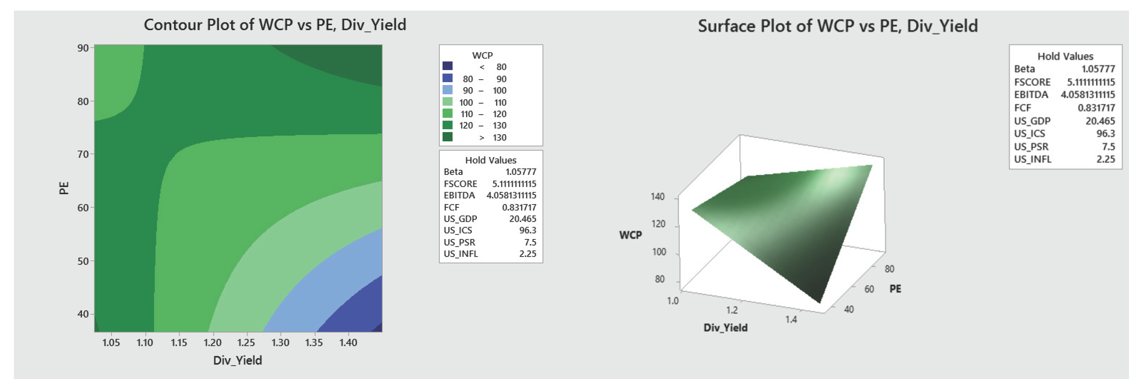
Figure A2.
Showing the Contour Plot (left) and Surface Plot (right) of The Estimated Response Surface as Div_Yield and FCF Vary, Keeping Other Indicators Fixed at a Specific Level.
Figure A2.
Showing the Contour Plot (left) and Surface Plot (right) of The Estimated Response Surface as Div_Yield and FCF Vary, Keeping Other Indicators Fixed at a Specific Level.
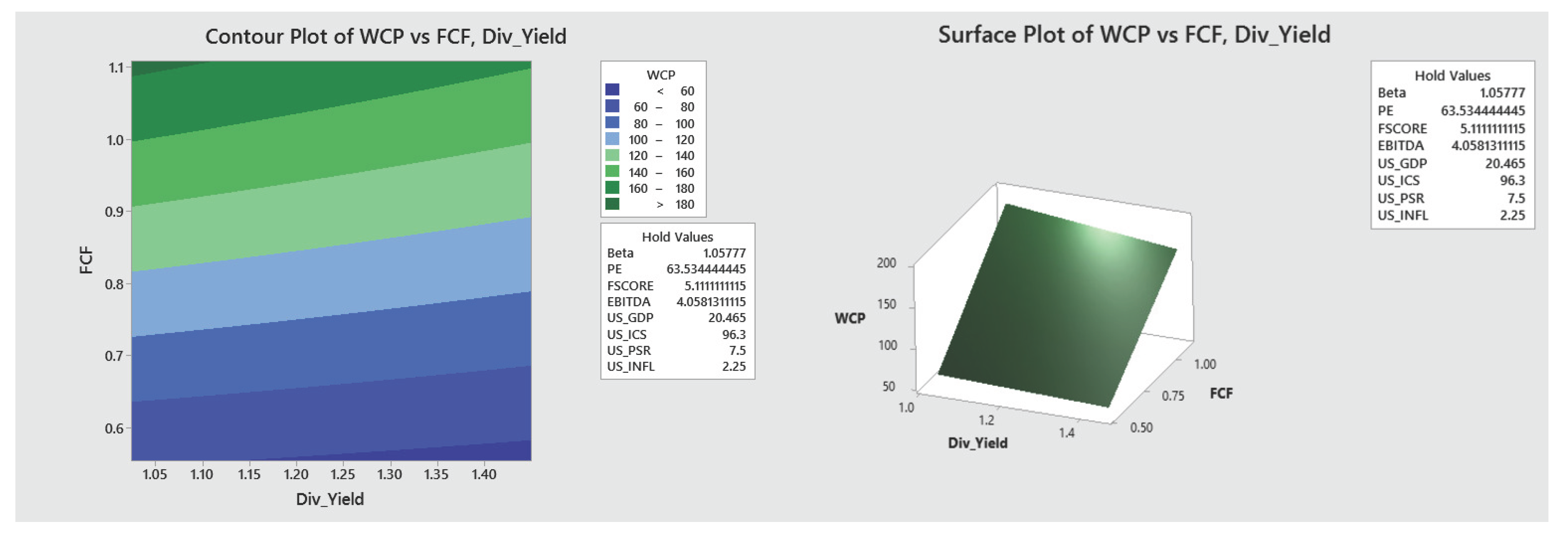
Figure 7 above describes how the response WCP changes with the variation of Div_Yield and FCF. The response WCP is maximized (light green region, $120-$160) where FCF remains approximately within the interval [.9,1] throughout the range of Div_Yield. The WCP has an increasing pattern with the increase of FCF. Any financial investor willing to invest in the healthcare segment of S&P 500 may use the above visual representation to select the stocks whose FCF falls within the specified range.
Figure A3.
Showing the Contour Plot (left) and Surface Plot (right) of The Estimated Response Surface as Beta and PE Vary, Keeping Other Indicators Fixed at a Specific Level.
Figure A3.
Showing the Contour Plot (left) and Surface Plot (right) of The Estimated Response Surface as Beta and PE Vary, Keeping Other Indicators Fixed at a Specific Level.
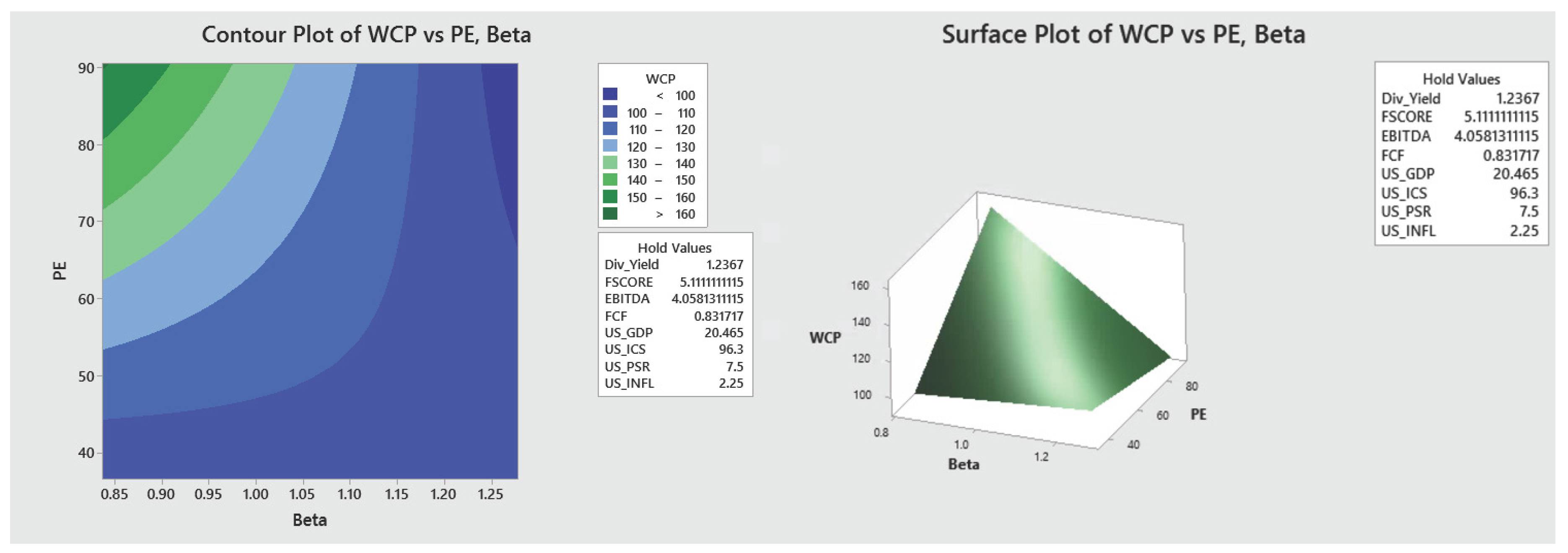
Figure 8 above describes how the response WCP changes with the variation of Beta and PE. The response WCP is maximized ($140-$160) where Beta remains approximately less than .95 and PE remains approximately more than 71. There is an increasing pattern in WCP with increasing PE ratio and decreasing Beta risk. Hence, we can infer that the response is maximized when the Beta risk is low and the PE ratio is high.
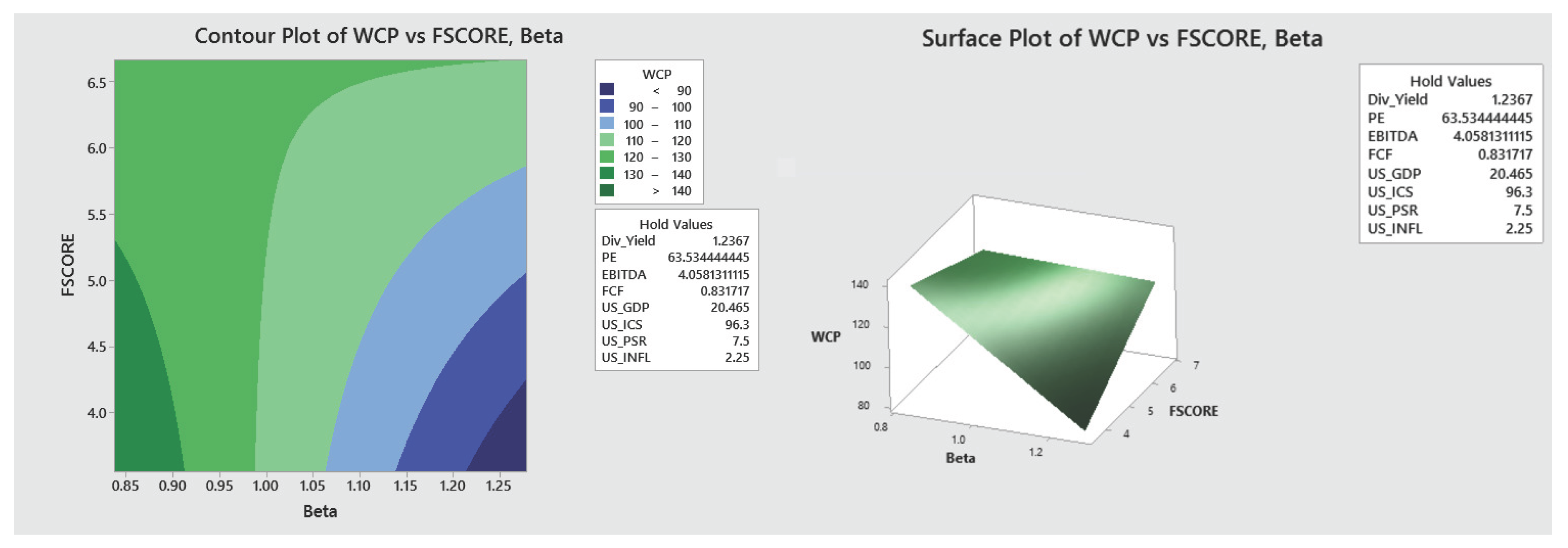
Figure 9 illustrates that the estimated WCP is maximized in the region where Beta lies approximately below .91 and FSCORE lies approximately at 5.5 and below. Also, WCP has an increasing pattern as we keep on decreasing Beta gradually.
Figure A4.
Showing the Contour Plot (left) and Surface Plot (right) of The Estimated Response Surface as Beta and FSCORE Vary, Keeping Other Indicators Fixed at a Specific Level.
Figure A4.
Showing the Contour Plot (left) and Surface Plot (right) of The Estimated Response Surface as Beta and FSCORE Vary, Keeping Other Indicators Fixed at a Specific Level.
From the following Figure 10, we see that the estimated response WCP is maximized in the region where Beta lies approximately below 1.17 and FCF lies approximately within the interval [0.8, 1]. WCP keeps on increasing with the increase of FCF, and it gets maximized as Beta decreases.
Figure A5.
Showing the Contour Plot (left) and Surface Plot (right) of The Estimated Response Surface as Beta and FCF Vary, Keeping Other Indicators Fixed at a Specific Level.
Figure A5.
Showing the Contour Plot (left) and Surface Plot (right) of The Estimated Response Surface as Beta and FCF Vary, Keeping Other Indicators Fixed at a Specific Level.
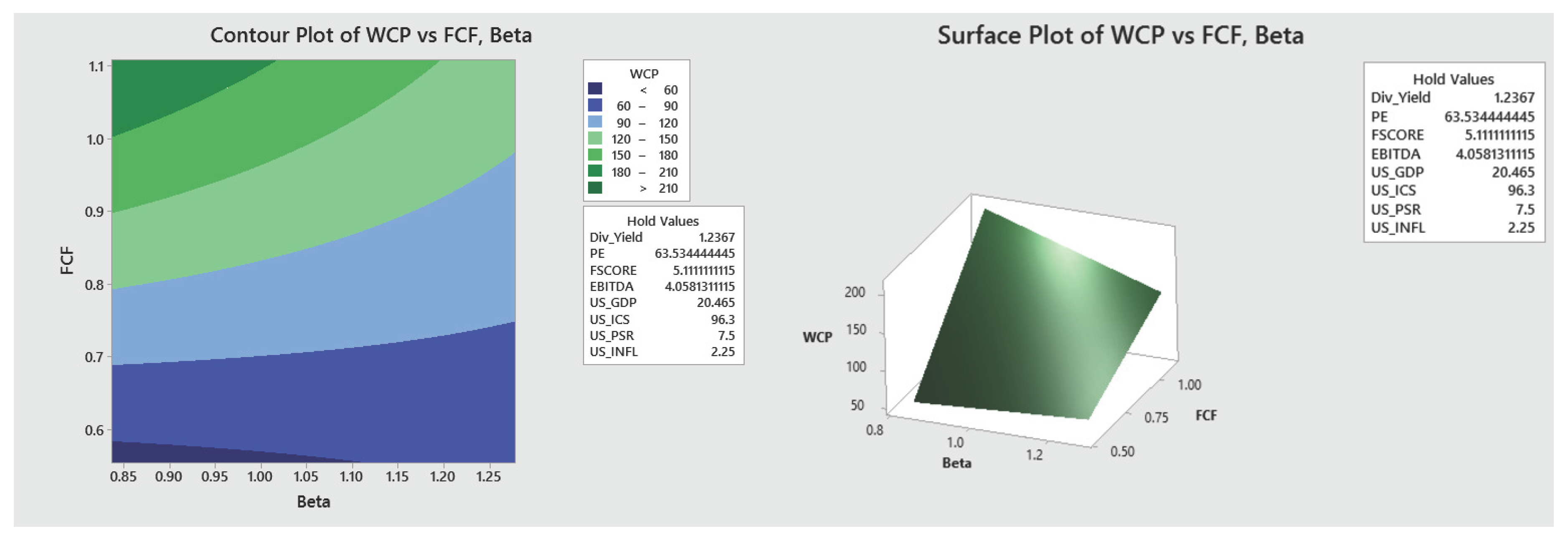
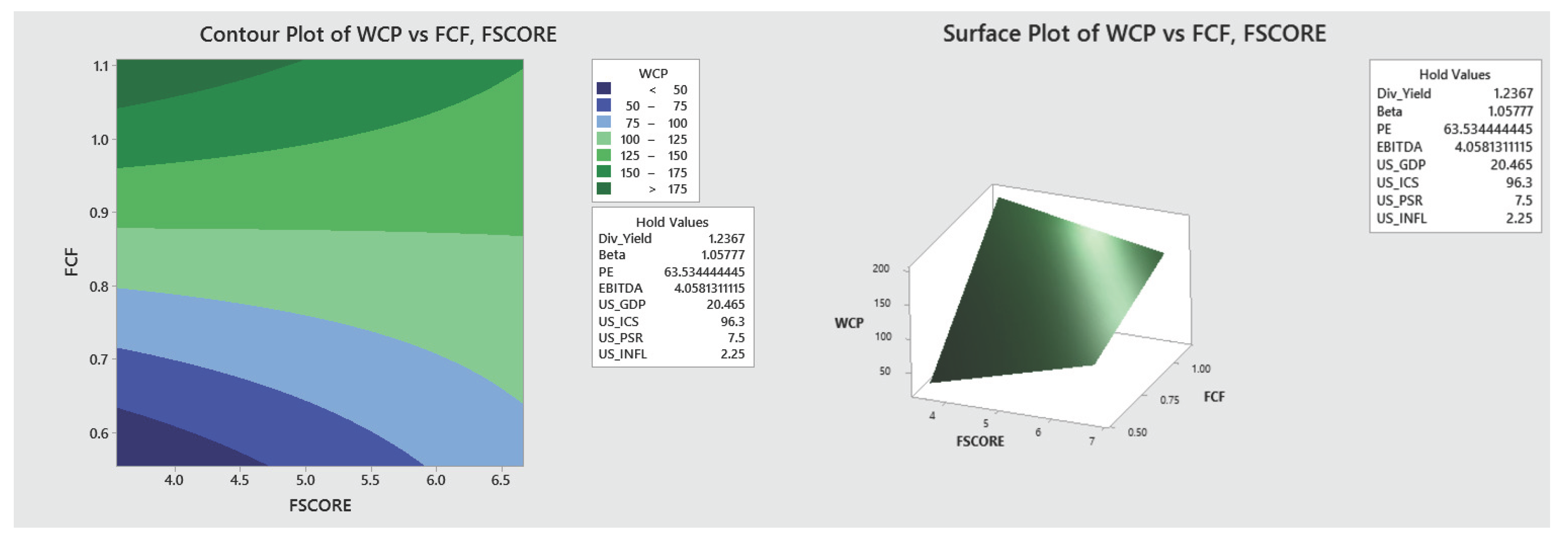
Figure 11 below describes how the response WCP changes with the variation of FSCORE and FCF, keeping other indicators at the desired level. The response WCP is maximized, where FCF remains approximately within the interval [.95,1.05] throughout the range of FSCORE. WCP attains its minimum value in the region where both FSCORE and FCF are low (deep blue). Gradually it increases with the increase in both indicators as desired.
Figure A6.
Showing the Contour Plot (left) and Surface Plot (right) of The Estimated Response Surface as FSCORE and FCF Vary, Keeping Other Indicators Fixed at a Specific Level.
Figure A6.
Showing the Contour Plot (left) and Surface Plot (right) of The Estimated Response Surface as FSCORE and FCF Vary, Keeping Other Indicators Fixed at a Specific Level.
Although financial and economic indicator-based stock price optimization models provide investors and portfolio managers with insightful information, their use has notable limitations. These models might suffer from overfitting, reliance on lagging or incomplete data, and difficulty capturing qualitative or unexpected market events. Model accuracy may also be compromised by crowd-driven trading patterns, behavioral factors, and regulatory changes. Furthermore, questions concerning fair access and transparency are raised by the growing usage of intricate or opaque algorithms. As a result, even if these models might improve market efficiency and decision-making, their results should be carefully comprehended and reinforced by sound risk management techniques and professional judgment.
Appendix B. Supplementary Material
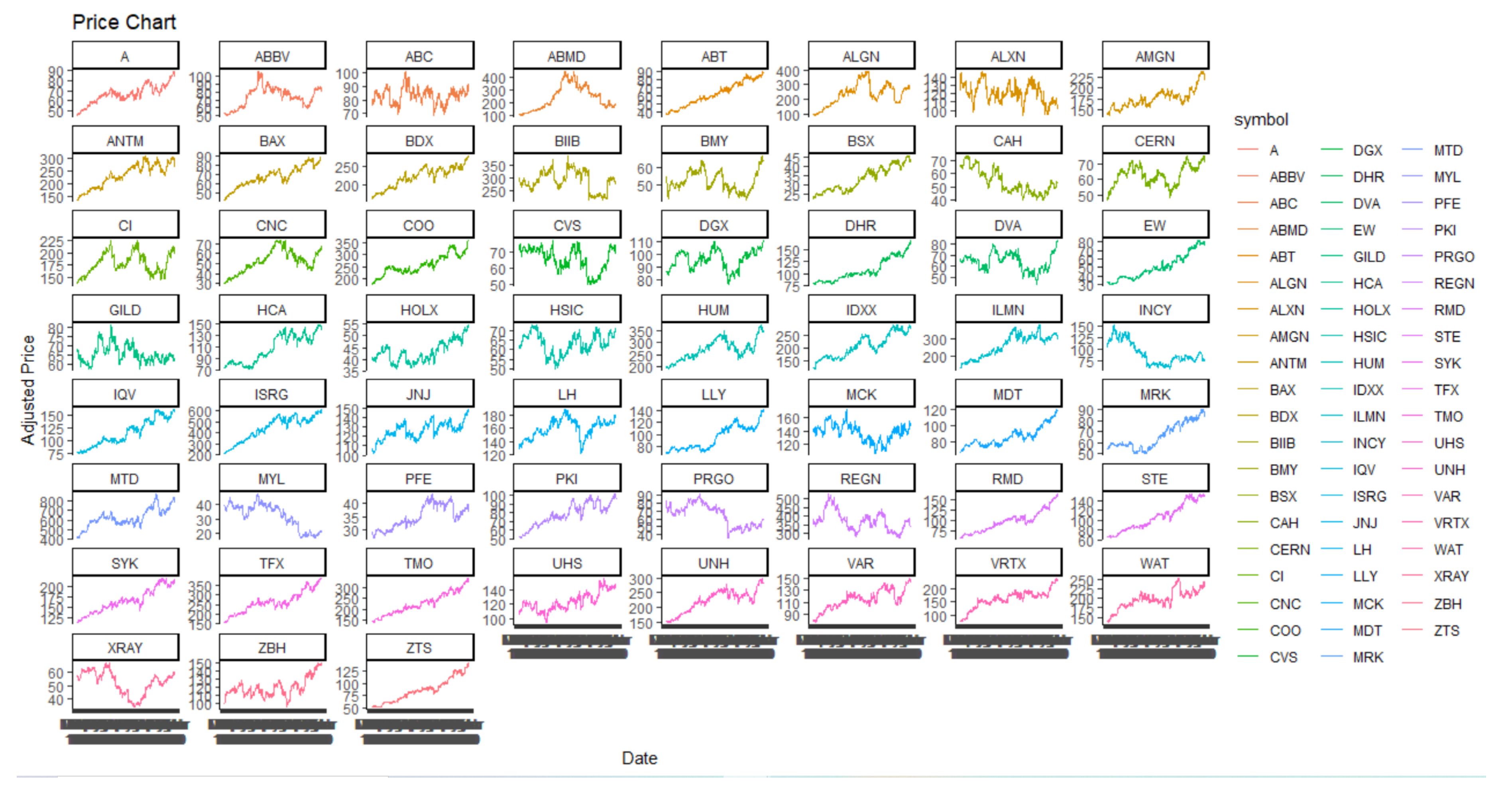
The dataset that was used to build our analytical model was obtained from Yahoo Finance (https://finance.yahoo.com/, and the indicators were combined together from the U.S Bureau of Economic Analysis (https://www.bea.gov/, and the US Bureau of Labor Statistics (https://www.bls.gov/). The information (closing price) on the 59 stocks belonging to the HBS, was put together with the financial, and economic indicators to structure the dataset for analysis. In structuring the weekly database of the index, we collected weekly information about the indicators for all 59 companies listed in the Healthcare Sector Index of the S&P 500 and averaged the weekly data of each indicator corresponding to these companies. The following price chart is based on the 59 healthcare stocks of the S&P 500. Our data includes the information from 01/01/2012 to 12/31/2018.
Figure A7.
Price Chart of The 59 Health Care Stocks.
References
- Fama, E.F.; French, K.R. The cross-section of expected stock returns. the Journal of Finance 1992, 47, 427–465. [Google Scholar]
- Piotroski, J.D. Value investing: The use of historical financial statement information to separate winners from losers. Journal of Accounting Research 2000, 1–41. [Google Scholar] [CrossRef]
- Chen, N.F.; Roll, R.; Ross, S.A. Economic forces and the stock market. Journal of business 1986, 383–403. [Google Scholar] [CrossRef]
- Fama, E.F. Stock returns, expected returns, and real activity. The journal of finance 1990, 45, 1089–1108. [Google Scholar] [CrossRef]
- Rapach, D.; Zhou, G. Forecasting stock returns. In Handbook of economic forecasting; Elsevier, 2013; Vol. 2, pp. 328–383.
- Siegel, J.J.; Schwartz, J.D. Long-term returns on the original S&P 500 companies. Financial Analysts Journal 2006, 62, 18–31. [Google Scholar]
- Sakaki, H. Oil price shocks and the equity market: Evidence for the S&P 500 sectoral indices. Research in International Business and Finance 2019, 49, 137–155. [Google Scholar] [CrossRef]
- Kawaller, I.G.; Koch, P.D.; Koch, T.W. The temporal price relationship between S&P 500 futures and the S&P 500 index. The Journal of Finance 1987, 42, 1309–1329. [Google Scholar]
- Dieleman, J.L.; Cao, J.; Chapin, A.; Chen, C.; Li, Z.; Liu, A.; Horst, C.; Kaldjian, A.; Matyasz, T.; Scott, K.W.; et al. US health care spending by payer and health condition, 1996-2016. Jama 2020, 323, 863–884. [Google Scholar] [CrossRef] [PubMed]
- Chen, M.P.; Chen, W.Y.; Tseng, T.C. Co-movements of returns in the health care sectors from the US, UK, and Germany stock markets: Evidence from the continuous wavelet analyses. International Review of Economics & Finance 2017, 49, 484–498. [Google Scholar] [CrossRef]
- Ge, Q. Enhancing stock market Forecasting: A hybrid model for accurate prediction of S&P 500 and CSI 300 future prices. Expert Systems with Applications 2025, 260, 125380. [Google Scholar]
- Alamu, O.S.; Siam, M.K. Stock price prediction and traditional models: An approach to achieve short-, medium-and long-term goals. arXiv 2024, arXiv:2410.07220. [Google Scholar] [CrossRef]
- Chakraborty, A.; Tsokos, C. A Stock Optimization Problem in Finance: Understanding Financial and Economic Indicators through Analytical Predictive Modeling. Mathematics 2024, 12. [Google Scholar] [CrossRef]
- Lashgari, A. Assessing text mining and technical analyses on forecasting financial time series. arXiv 2023, arXiv:2304.14544. [Google Scholar] [CrossRef]
- Sangwan, V.; Kumar, V.; Christopher, V.B. Contrasting the efficiency of stock price prediction models using various types of LSTM models aided with sentiment analysis. In Proceedings of the AIP Conference Proceedings. AIP Publishing, 2024, Vol. 3075.
- Kumar, S.; Ghildayal, N.S.; Shah, R.N. Examining quality and efficiency of the US healthcare system. International journal of health care quality assurance 2011, 24, 366–388. [Google Scholar] [CrossRef]
- Raghupathi, V.; Raghupathi, W. Healthcare expenditure and economic performance: insights from the United States data. Frontiers in public health 2020, 8, 156. [Google Scholar] [CrossRef]
- Kumar, R. Valuation: theories and concepts; Academic Press, 2015.
- McManus, I.; Ap Gwilym, O.; Thomas, S. The role of payout ratio in the relationship between stock returns and dividend yield. Journal of Business Finance & Accounting 2004, 31, 1355–1387. [Google Scholar] [CrossRef]
- Lajevardi, S. A study on the effect of P/E and PEG ratios on stock returns: Evidence from Tehran Stock Exchange. Management Science Letters 2014, 4, 1401–1410. [Google Scholar] [CrossRef]
- Tang, G.Y.; Shum, W.C. The conditional relationship between beta and returns: Recent evidence from international stock markets. International Business Review 2003, 12, 109–126. [Google Scholar] [CrossRef]
- Walkshäusl, C. Piotroski’s FSCORE: international evidence. Journal of Asset Management 2020, 21, 106–118. [Google Scholar] [CrossRef]
- Kansanen, A.; et al. Effectiveness of Piotroski F-Score for Finnish Stocks. 2016.
- Kusowska, M.; et al. Assessment of efficiency of Piotroski F-Score strategy in the Warsaw Stock Exchange. Przedsiębiorstwo we współczesnej gospodarce–teoria i praktyka 2021, 32, 47–59. [Google Scholar]
- Nissim, D. EBITDA, EBITA, or EBIT? Columbia Business School Research Paper, 2019, 17–71.
- Rozenbaum, O. EBITDA and managers’ investment and leverage choices. Contemporary Accounting Research 2019, 36, 513–546. [Google Scholar] [CrossRef]
- Drake, P.P. What is free cash flow and how do I calculate it? James Madison 2005. [Google Scholar]
- Sharma, G.D.; Mahendru, M. Impact of macro-economic variables on stock prices in India. Global Journal of Management and Business Research 2010, 10. [Google Scholar]
- Büyüksalvarci, A.; Abdioglu, H. The causal relationship between stock prices and macroeconomic variables: A case study for Turkey. Journal of Economic & Management Perspectives 2010, 4, 601. [Google Scholar]
- Mukherjee, T.K.; Naka, A. Dynamic relations between macroeconomic variables and the Japanese stock market: an application of a vector error correction model. Journal of financial Research 1995, 18, 223–237. [Google Scholar] [CrossRef]
- Osamwonyi, I.O.; Evbayiro-Osagie, E.I. The relationship between macroeconomic variables and stock market index in Nigeria. Journal of Economics 2012, 3, 55–63. [Google Scholar] [CrossRef]
- Singh, T.; Mehta, S.; Varsha, M. Macroeconomic factors and stock returns: Evidence from Taiwan. Journal of economics and international finance 2011, 3, 217. [Google Scholar]
- Jareño, F.; Negrut, L.; et al. US stock market and macroeconomic factors. Journal of Applied Business Research (JABR) 2016, 32, 325–340. [Google Scholar] [CrossRef]
- Lemmon, M.; Portniaguina, E. Consumer confidence and asset prices: Some empirical evidence. The Review of Financial Studies 2006, 19, 1499–1529. [Google Scholar] [CrossRef]
- Howrey, E. The Predictive Power of the Index of Consumer Sentiment. Brookings Papers on Economic Activity 2001, 32, 175–216. [Google Scholar] [CrossRef]
- Singal, M. Effect of consumer sentiment on hospitality expenditures and stock returns. International Journal of Hospitality Management 2012, 31, 511–521. [Google Scholar] [CrossRef]
- Tootell, G.M.; et al. Globalization and US inflation. New England Economic Review 1998, 21–34. [Google Scholar]
- Antonakakis, N.; Gupta, R.; Tiwari, A.K. Has the correlation of inflation and stock prices changed in the United States over the last two centuries? Research in International Business and Finance 2017, 42, 1–8. [Google Scholar] [CrossRef]
- Albulescu, C.T.; Aubin, C.; Goyeau, D. Stock prices, inflation and inflation uncertainty in the US: testing the long-run relationship considering Dow Jones sector indexes. Applied Economics 2017, 49, 1794–1807. [Google Scholar] [CrossRef]
- Friedrich, C.; Selcuk, P. The impact of globalization and digitalization on the Phillips Curve. Technical report, Bank of Canada Staff Working Paper, 2022.
- Van Rooij, M.; Lusardi, A.; Alessie, R. Financial literacy and stock market participation. Journal of Financial economics 2011, 101, 449–472. [Google Scholar] [CrossRef]
- González-Estrada, E.; Cosmes, W. Shapiro–Wilk test for skew normal distributions based on data transformations. Journal of Statistical Computation and Simulation 2019, 89, 3258–3272. [Google Scholar] [CrossRef]
- Royston, P. Approximating the Shapiro-Wilk W-test for non-normality. Statistics and computing 1992, 2, 117–119. [Google Scholar] [CrossRef]
- Yeo, I.K.; Johnson, R.A. A new family of power transformations to improve normality or symmetry. Biometrika 2000, 87, 954–959. [Google Scholar] [CrossRef]
- Farnum, N.R. Using JOHNSON curves to describe non-normal ROCESS data. Quality Engineering 1996, 9, 329–336. [Google Scholar] [CrossRef]
- Polansky, A.M.; Chou, Y.M.; Mason, R.L. An algorithm for fitting Johnson transformations to non-normal data. Journal of quality technology 1999, 31, 345–350. [Google Scholar] [CrossRef]
- Fashoto, S.G.; Mbunge, E.; Ogunleye, G.; den Burg, J.V. Implementation of machine learning for predicting maize crop yields using multiple linear regression and backward elimination. Malaysian Journal of Computing (MJoC) 2021, 6, 679–697. [Google Scholar] [CrossRef]
- Samal, A.R.; Mohanty, M.K.; Fifarek, R.H. Backward elimination procedure for a predictive model of gold concentration. Journal of Geochemical Exploration 2008, 97, 69–82. [Google Scholar] [CrossRef]
- Rustam, F.; Reshi, A.A.; Mehmood, A.; Ullah, S.; On, B.W.; Aslam, W.; Choi, G.S. COVID-19 future forecasting using supervised machine learning models. IEEE access 2020, 8, 101489–101499. [Google Scholar] [CrossRef]
- Wong, T.T.; Yeh, P.Y. Reliable accuracy estimates from k-fold cross validation. IEEE Transactions on Knowledge and Data Engineering 2019, 32, 1586–1594. [Google Scholar] [CrossRef]
- Berrar, D.; et al. Cross-Validation., 2019.
- de Lima Lemos, R.A.; Silva, T.C.; Tabak, B.M. Propension to customer churn in a financial institution: A machine learning approach. Neural Computing and Applications 2022, 34, 11751–11768. [Google Scholar] [CrossRef] [PubMed]
- Yoon, J. Forecasting of real GDP growth using machine learning models: Gradient boosting and random forest approach. Computational Economics 2021, 57, 247–265. [Google Scholar] [CrossRef]
- Thakkar, A.; Chaudhari, K. A comprehensive survey on portfolio optimization, stock price and trend prediction using particle swarm optimization. Archives of Computational Methods in Engineering 2021, 28, 2133–2164. [Google Scholar] [CrossRef]
- Gülmez, B. Stock price prediction with optimized deep LSTM network with artificial rabbits optimization algorithm. Expert Systems with Applications 2023, 227, 120346. [Google Scholar] [CrossRef]
- Chen, T.; He, T.; Benesty, M.; Khotilovich, V.; Tang, Y.; Cho, H.; Chen, K.; Mitchell, R.; Cano, I.; Zhou, T.; et al. Xgboost: extreme gradient boosting. R package version 0.4-2 2015, 1, 1–4. [Google Scholar]
- Osman, A.I.A.; Ahmed, A.N.; Chow, M.F.; Huang, Y.F.; El-Shafie, A. Extreme gradient boosting (Xgboost) model to predict the groundwater levels in Selangor Malaysia. Ain Shams Engineering Journal 2021, 12, 1545–1556. [Google Scholar] [CrossRef]
- Wu, J.; Wang, Y.G.; Burrage, K.; Tian, Y.C.; Lawson, B.; Ding, Z. An improved firefly algorithm for global continuous optimization problems. Expert Systems with Applications 2020, 149, 113340. [Google Scholar] [CrossRef]
- Melnik, A.; Shumetov, V.; Kondrashin, B.; Mikhaylov, M. Use of Harrington’s desirability function in wheat grain quality assessment. In Proceedings of the IOP Conference Series: Earth and Environmental Science. IOP Publishing, 2020, Vol. 422:1.
- Palandi Cardoso, R.; da Motta Reis, J.S.; Werderits Silva, D.E.; Medeiros de Barros, J.G.; de Souza Sampaio, N.A. How to perform a simultaneous optimization with several response variables. GeSec: Revista de Gestao e Secretariado 2023, 14. [Google Scholar]
- Nazarpour, M.; Taghizadeh-Alisaraei, A.; Asghari, A.; Abbaszadeh-Mayvan, A.; Tatari, A. Optimization of biohydrogen production from microalgae by response surface methodology (RSM). Energy 2022, 253, 124059. [Google Scholar] [CrossRef]
- Kumari, M.; Gupta, S.K. Response surface methodological (RSM) approach for optimizing the removal of trihalomethanes (THMs) and its precursor’s by surfactant modified magnetic nanoadsorbents (sMNP)-An endeavor to diminish probable cancer risk. Scientific Reports 2019, 9, 18339. [Google Scholar] [CrossRef]
- Derringer, G.; Suich, R. Simultaneous optimization of several response variables. Journal of quality technology 1980, 12, 214–219. [Google Scholar] [CrossRef]
- Benhayoun, N.; Chairi, I.; El Gonnouni, A.; Lyhyaoui, A. Financial intelligence in prediction of firm’s creditworthiness risk: evidence from support vector machine approach. Procedia Economics and Finance 2013, 5, 103–112. [Google Scholar] [CrossRef]
- Chakraborty, A.; Tsokos, C.P. An AI-driven Predictive Model for Pancreatic Cancer Patients Using Extreme Gradient Boosting. Journal of Statistical Theory and Applications 2023, 22, 262–282. [Google Scholar] [CrossRef]
- Malyshenko, K.A.; Shafiee, M.M.; Malyshenko, V.A.; Anashkina, M.V. Dynamics of the securities market in the information asymmetry context: developing a methodology for emerging securities markets. Global Business and Economics Review 2021, 25, 89–114. [Google Scholar] [CrossRef]
- Chakraborty, A.; Tsokos, C. A Stock Optimization Problem in Finance: Understanding Financial and Economic Indicators through Analytical Predictive Modeling. Mathematics 2024, 12, 2407. [Google Scholar] [CrossRef]
- Grassi, S.; Proietti, T.; Frale, C.; Marcellino, M.; Mazzi, G. EuroMInd-C: A disaggregate monthly indicator of economic activity for the Euro area and member countries. International Journal of Forecasting 2015, 31, 712–738. [Google Scholar] [CrossRef]
- Tao, L.; Xiaojing, G.; Ningning, Z. Notice of Retraction: The principal component analysis and evaluation of financial performance for enterprises based on cash flow information. In Proceedings of the 2010 IEEE International Conference on Advanced Management Science (ICAMS 2010). IEEE, 2010, Vol. 3, pp. 291–296.
- Jiang, W. Applications of deep learning in stock market prediction: recent progress. Expert Systems with Applications 2021, 184, 115537. [Google Scholar] [CrossRef]
- Gao, Y.; Wang, R.; Zhou, E. Stock prediction based on optimized LSTM and GRU models. Scientific Programming 2021, 2021, 4055281. [Google Scholar] [CrossRef]
- Peng, L.; Chen, K.; Li, N. Predicting stock movements: using multiresolution wavelet reconstruction and deep learning in neural networks. Information 2021, 12, 388. [Google Scholar] [CrossRef]
- Dietterich, T. Overfitting and undercomputing in machine learning. ACM computing surveys (CSUR) 1995, 27, 326–327. [Google Scholar] [CrossRef]
- Jabbar, H.; Khan, R.Z. Methods to avoid over-fitting and under-fitting in supervised machine learning (comparative study). Computer Science, Communication and Instrumentation Devices 2015, 70, 978–981. [Google Scholar]
- Hou, K.; Xue, C.; Zhang, L. Digesting anomalies: An investment approach. The Review of Financial Studies 2015, 28, 650–705. [Google Scholar] [CrossRef]
- Reji, M.; Kumar, R. Response surface methodology (RSM): An overview to analyze multivariate data. Indian J. Microbiol. Res 2022, 9, 241–248. [Google Scholar]
- Breig, S.J.M.; Luti, K.J.K. Response surface methodology: A review on its applications and challenges in microbial cultures. Materials Today: Proceedings 2021, 42, 2277–2284. [Google Scholar] [CrossRef]
- Sholichah, F.; Asfiah, N.; Ambarwati, T.; Widagdo, B.; Ulfa, M.; Jihadi, M. The effects of profitability and solvability on stock prices: Empirical evidence from Indonesia. The Journal of Asian Finance, Economics and Business 2021, 8, 885–894. [Google Scholar]
- Pando, V.; San-Jose, L.A.; Sicilia, J.; Alcaide-Lopez-de Pablo, D. Maximization of the return on inventory management expense in a system with price-and stock-dependent demand rate. Computers & Operations Research 2021, 127, 105134. [Google Scholar]
Figure 1.
Q-Q Plot Of The Response WCP.
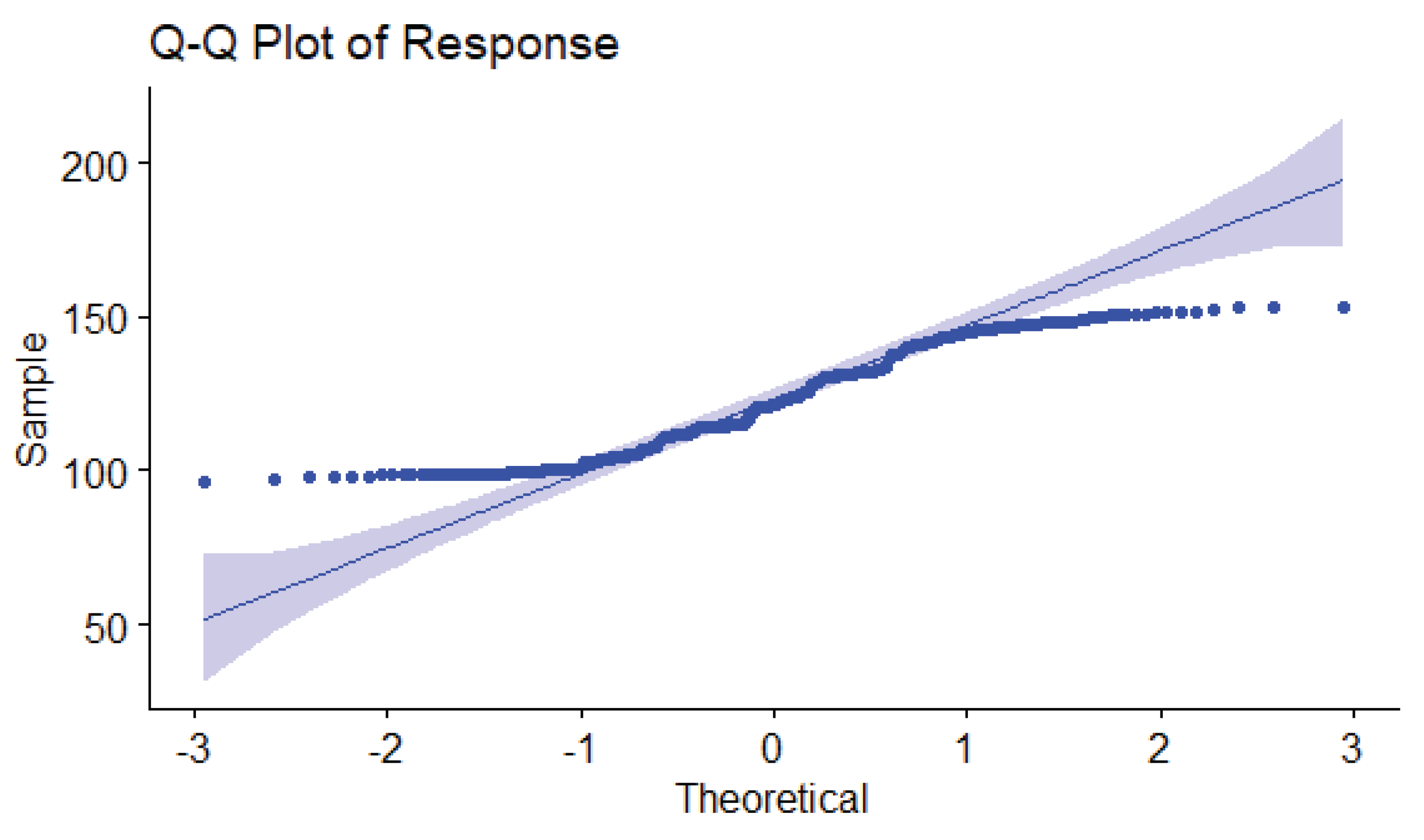
Figure 2.
Normality of Studentized Residual Plot.
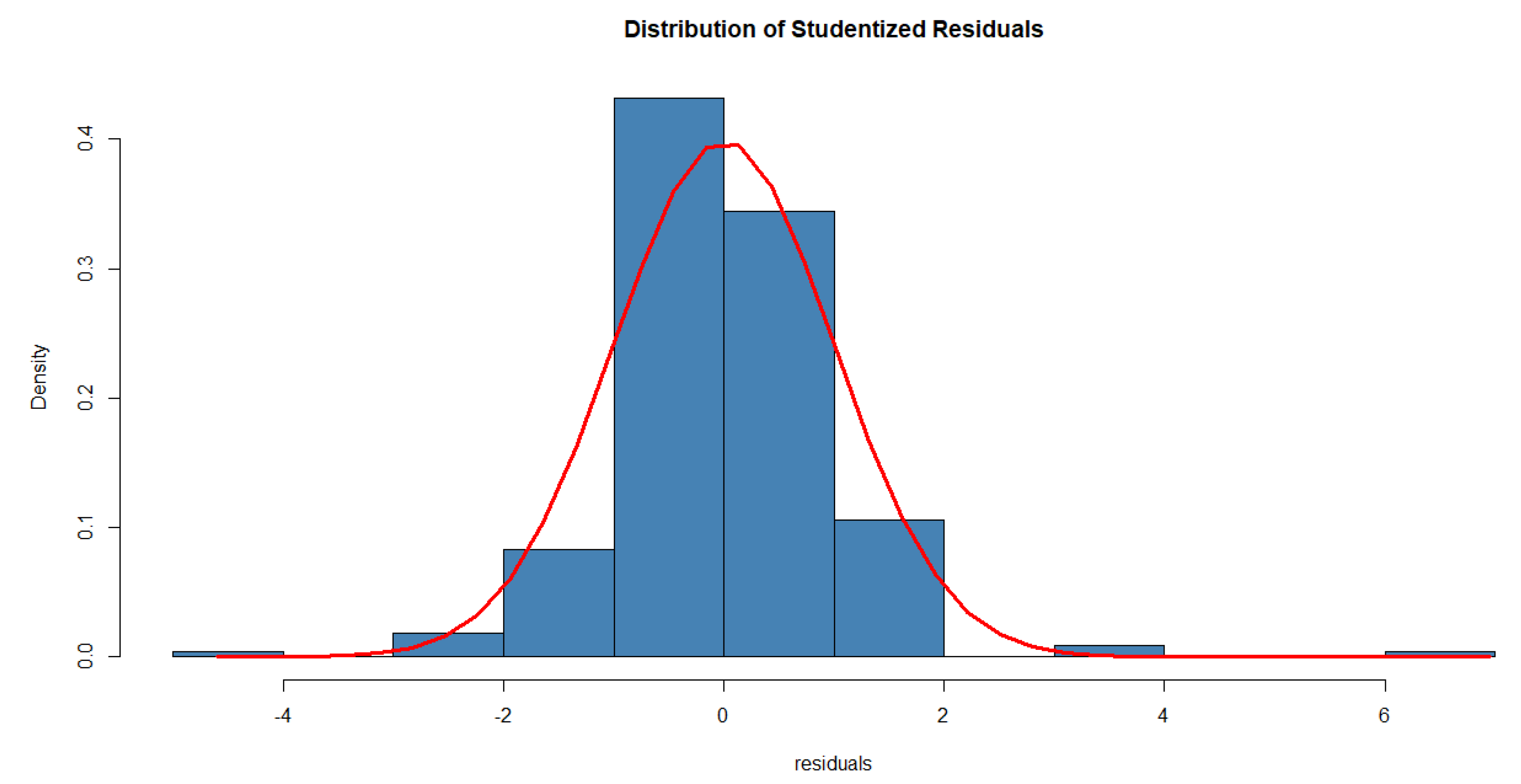
Figure 4.
Brief Illustration Of Repeated Ten Fold Cross Validation.
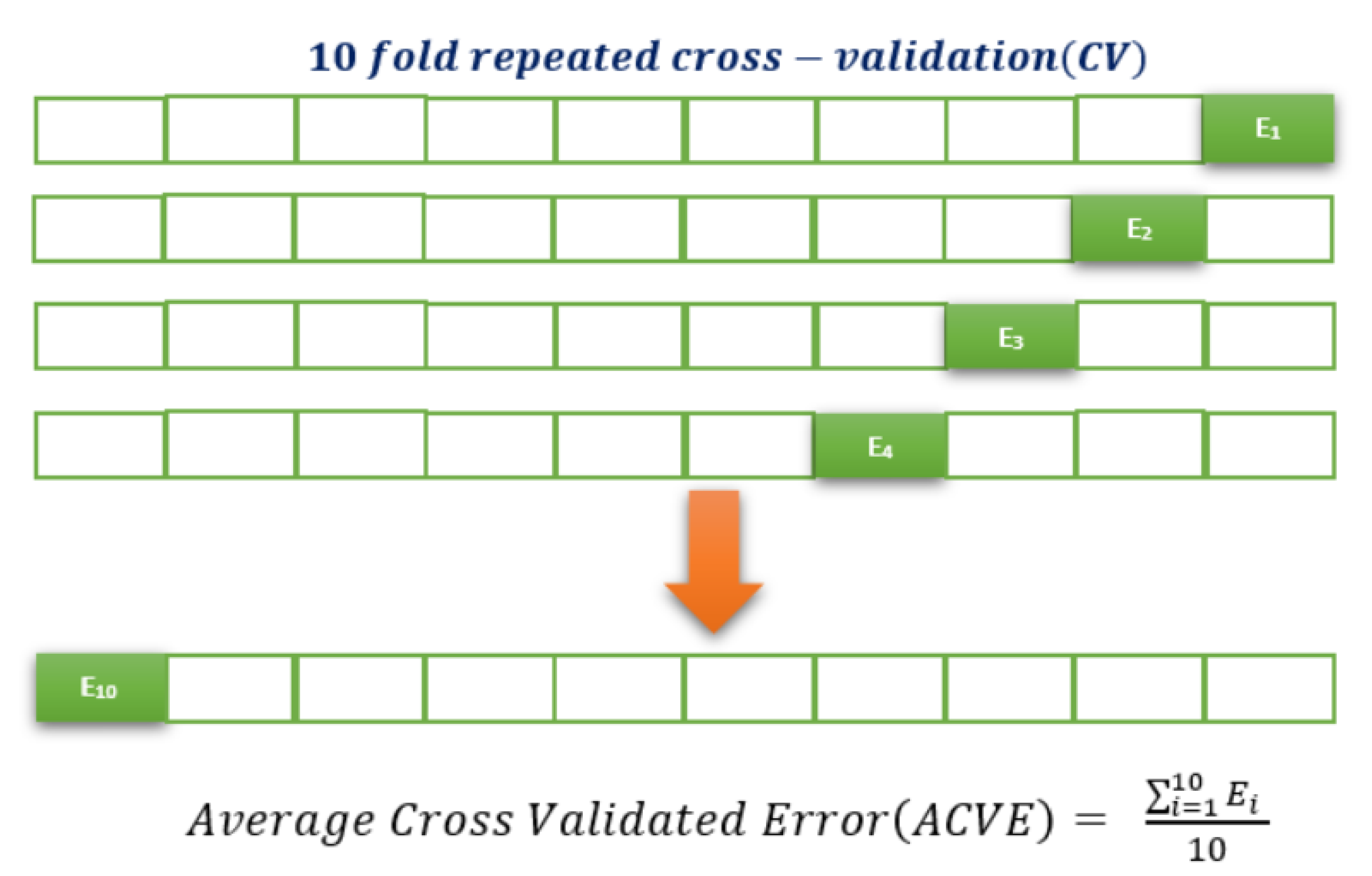
Figure 5.
Variation of and in Different Folds.
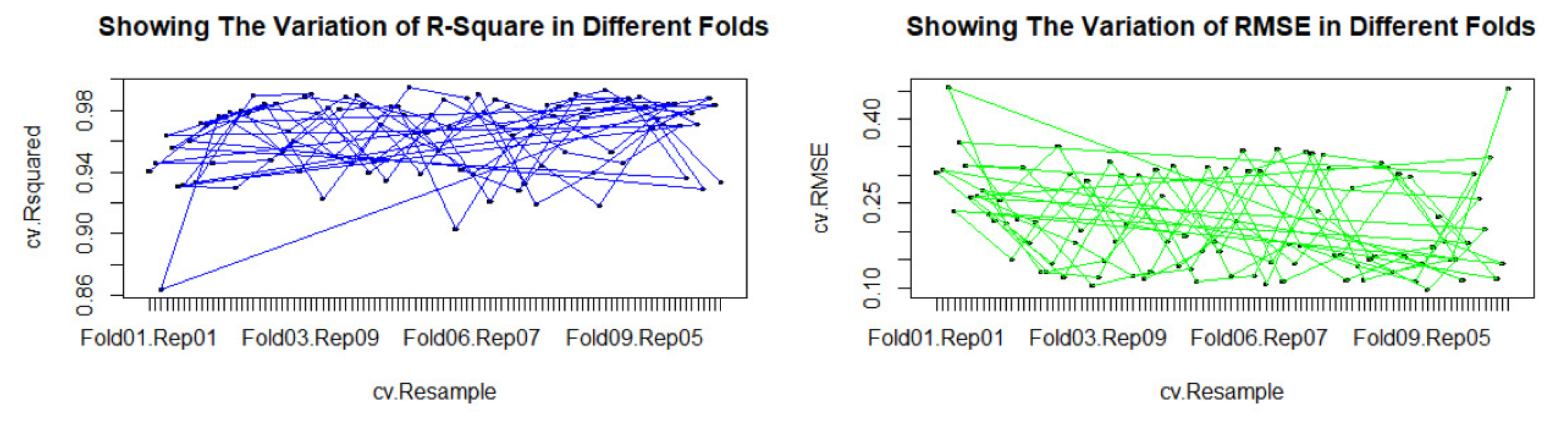

Table 1.
Ranking of the Indicators and the Interactions with Respect to the Percentage of Contribution to the Response WCP; The ∩ Indicates the Interaction between Two Indicators.
Table 1.
Ranking of the Indicators and the Interactions with Respect to the Percentage of Contribution to the Response WCP; The ∩ Indicates the Interaction between Two Indicators.
| Rank | Indicators | Contr.(%) | Rank | Indicators | Contr.(%) |
| 1 | 4.53 | 21 | 2.41 | ||
| 2 | 4.15 | 22 | 2.35 | ||
| 3 | 3.89 | 23 | 2.27 | ||
| 4 | 3.63 | 24 | 2.24 | ||
| 5 | 3.41 | 25 | 2.20 | ||
| 6 | 3.34 | 26 | 2.18 | ||
| 7 | 3.34 | 27 | 2.14 | ||
| 8 | 3.27 | 28 | 2.10 | ||
| 9 | 3.07 | 29 | 2.07 | ||
| 10 | 3.05 | 30 | 2.02 | ||
| 11 | 3.03 | 31 | 1.97 | ||
| 12 | 2.86 | 32 | 1.95 | ||
| 13 | 2.71 | 33 | 1.92 | ||
| 14 | 2.69 | 34 | 1.87 | ||
| 15 | 2.66 | 35 | 1.84 | ||
| 16 | 2.62 | 36 | 1.82 | ||
| 17 | 2.51 | 37 | 1.75 | ||
| 18 | 2.49 | 38 | 1.72 | ||
| 19 | 2.48 | 30 | 1.63 | ||
| 20 | 2.47 | 40 | 1.62 | ||
| 41 | 1.59 |
Table 2.
Ranking of the Indicators With Respect to The Percentage of Contribution to The Response Considering the Number of Occurrences in Model (2), Individually, and Interacting with Other Indicators.
Table 2.
Ranking of the Indicators With Respect to The Percentage of Contribution to The Response Considering the Number of Occurrences in Model (2), Individually, and Interacting with Other Indicators.
| Rank | Indicators | No. of Occurrence | Contr.(%) |
| 1 | 8 | 25.32 | |
| 2 | 8 | 20.14 | |
| 3 | 8 | 19.57 | |
| 4 | 7 | 19.23 | |
| 5 | 7 | 18.29 | |
| 6 | 8 | 18.23 | |
| 7 | 7 | 16.44 | |
| 8 | 8 | 16.41 | |
| 9 | 6 | 14.84 | |
| 10 | 5 | 12.66 |
Table 3.
Constraints On The Indicators Showing the Lower and Upper Limits.
| Indicators | Constraints |
Table 4.
Estimated Maximized Response with Optimum Values of the Indicators.
| Response & Indicators | Optimum Values |
|---|---|
| $155 | |
| 96.3 | |
| 7.5 | |
| 2.61 |
Table 5.
Some Useful Results Related to the Optimized Response.
| Estimated Maximized Value | $155 |
| Desirability | 1 |
| 98.84% | |
| 97.85% | |
| 95% CI | (139.57, 170.43) |
| 95% PI | (139.06, 170.94) |
Table 6.
Observed and Predicted Responses.
| Observations | Observed | Predicted | Observations | Observed | Predicted | |
| 1 | 155 | 156 | 63 | 136 | 141 | |
| 2 | 152 | 150 | 64 | 135 | 137 | |
| 5 | 151 | 149 | 72 | 153 | 148 | |
| 6 | 148 | 148 | 73 | 154 | 148 | |
| 13 | 141 | 145 | 81 | 143 | 147 | |
| 19 | 144 | 145 | 82 | 142 | 147 | |
| 20 | 143 | 146 | 83 | 140 | 141 | |
| 28 | 139 | 144 | 127 | 131 | 131 | |
| 29 | 138 | 144 | 148 | 123 | 126 | |
| 36 | 149 | 145 | 212 | 111 | 111 | |
| 37 | 150 | 144 | 213 | 111 | 112 | |
| 38 | 149 | 145 | 252 | 104 | 104 | |
| 39 | 152 | 148 | 255 | 104 | 107 | |
| 40 | 153 | 148 | 256 | 105 | 104 | |
| 41 | 153 | 155 | 272 | 98 | 100 |
Disclaimer/Publisher’s Note: The statements, opinions and data contained in all publications are solely those of the individual author(s) and contributor(s) and not of MDPI and/or the editor(s). MDPI and/or the editor(s) disclaim responsibility for any injury to people or property resulting from any ideas, methods, instructions or products referred to in the content. |
© 2025 by the authors. Licensee MDPI, Basel, Switzerland. This article is an open access article distributed under the terms and conditions of the Creative Commons Attribution (CC BY) license (http://creativecommons.org/licenses/by/4.0/).
Copyright: This open access article is published under a Creative Commons CC BY 4.0 license, which permit the free download, distribution, and reuse, provided that the author and preprint are cited in any reuse.


