
Submitted:
24 August 2025
Posted:
25 August 2025
You are already at the latest version
Abstract
For rendering visible phase gradients, we design a dark-field technique that exploits the cross-correlation of two coded masks. One mask is coded with the white and black versions of a Barker sequence. Its Babinet´s complementary screen is used as the second mask. We replicate the proposed masks for generating two binary complementary gratings. Phase gradients cause beam deviations, which generate cross-correlations between the two complementary gratings. We describe the cross-correlations using a compact matrix formulation. This description is amenable to numerical evaluation. The cross-correlations between complementary gratings are incorporated in the design of a dark-field, Lau interferometer.
Keywords:
barker sequences
; babinet complementary screens
; lau interferometry
; optical cross correlations
1. Introduction
Under coherent illumination, masks coded with periodic structures can create Fresnel diffraction patterns that are like the initial mask. This remarkable effect, known as the self-imaging phenomenon, appears in several ranges of the electromagnetic spectrum, as well as in matter waves [1,2,3,4,5,6].
The self-imaging phenomenon goes back to Talbot [7]. After several decades, the Talbot effect was applied for setting an optical interferometer [8,9,10]. Before the publication of Jahns and Lohmann [11], it was somehow unknown that under noncoherent illumination one can observe a related self-imaging phenomenon. Known as the Lau effect [12], the noncoherent version of the Talbot effect can also be applied for setting a nonconventional interferometer [13].
Nowadays, several authors have recognized that there is an akin phenomenon and related applications in temporal optics [14,15,16,17]. The Talbot-Lau phenomenon and their akin relatives have generated a myriad of contributions in several branches of applied optics [18,19,20,21].
Here, we focus our attention on the use of the Talbot-Lau effect for setting up a dark-ground, Lau interferometer. First, we consider the optical product between two Babinet’s complementary masks [22,23]. The first mask is coded with the black and white versions of a Barker sequence [24]. Its Babinet’s complementary screen is the second mask. We extend our previous description by employing two complementary gratings. These gratings are incorporated into a Lau interferometer, for obtaining a dark-field interferometer. If one employs tunable prisms, the dark-field interferometer can compensate for local beam deflections.
In Section 2, we discuss the use of the complementary masks for setting a dark-field sensor. In Section 3, we extend our previous proposal by discussing the generation of two complementary gratings. We employ a matrix formulation for describing the cross correlation between complementary gratings. And we numerically evaluate the cross correlation between the complementary gratings. In Section 4, the novel gratings are incorporated into a Lau interferometer. We note that the Lau interferometer works under noncoherent illumination. Then, the presence of phase gradients can be expressed in terms of an irradiance point spread function. In Section 5, we propose to use an average point spread function for describing the presence of randomly located prisms, which function as phase gradients. In Section 6, we summarize our contribution.
2. Barker-Babinet Complementary Masks
First, it is convenient to revisit the concept of complementary masks. A binary amplitude transmittance, say t(x, y), has the following property
In Equation (1) the lower-case letter n denotes a positive integer number, The amplitude transmittance of its binary complementary mask reads
In the Appendix A, we show that bc(x, y) also satisfies the condition in Equation (1). We note that Equation (2) is a necessary condition but is not a sufficient condition. For our current discussion, we also require that
In Figure 1, we portray the product of two complementary masks. In Figure 1 (a), we depict a mask coded with the sequence {0,0,1}. In Figure 1 (b), we display the complementary mask that is coded with the sequence {1,1,0}, which corresponds to the Barker sequence of length L = 3. In Figure 1 (c), we show the product of the two masks.
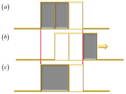
Now, as depicted in Figure 2, if the second mask is laterally shifted, one breaks the condition in Equation (3). This simple observation is used in what follows for setting an optical sensor of phase gradients.
Under noncoherent illumination, one can implement optically the product between complementary masks by employing the setup in Figure 3. A single lens images (with magnification M = - 1) an initial mask on its complementary mask.
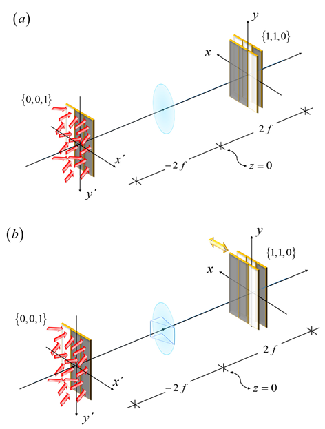
Figure 3 Imaging device for implementing the mathematical operation in Figure 1, for two complementary masks, one is coded with the Barker sequence of length L = 3. In (a) the complementary mask produces zero light throughput, as in Equation (3). In (b), a phase gradient breaks the condition for zero throughput.
In Figure 3 (a), we illustrate that in the absence of phase gradients,the light throughput is equal to zero. In Figure 3 (b), we depict that a phase gradient introduces a lateral shift of the image. Hence, the presence of the phase gradient breaks the zero-throughput condition. Next, we discuss a simple mathematical description of the above heuristic pictorials.
3. Dark Background Sensor
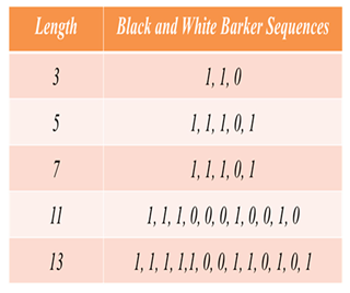
For clarifying our notation, we indicate that the initial binary mask, b(x, y), is coded with the black and white version of the Barker sequences. The number of elements in the sequence is denoted as the length L. In mathematical terms,
In Eq.(4) the upper-case letter “L” stands for the length of the Barker sequence. And the upper-case letter “D” denotes the support of the binary mask. In Table 1, we show the numerical values of five members the binary version of the Barker sequences.
The Babinet complementary screen has the following amplitude transmittance
Now, from equations (4) and (5) we obtain the product
From Equation (6) we note that the product is equal to zero, each time that if the coefficient Bn is equal to zero. And the product is also equal to zero each time that the coefficient Bn is equal to unity.
For the sake of clarity, we describe in simple terms the optical setup in Figure 3 . At the source plane, the irradiance distribution is
In Equation (7), the composing source points are located at
In Equations (7) and (8) the lower-case letter “s” denotes an integer number. Next, we include the presence of a prismatic lateral displacement, caused by an angular deviation θ. At the image plane the irradiance distribution is
At the image plane, we place the second mask. Its irradiance transmittance is
Hence, after the second mask, the light throughput reads
By substituting Equations (9) and (10) in Equation (11) we obtain
It is clear, from Equation (12), that if θ = 0, then we have the condition in Equation (3). And if one evaluates Equation (12) at integer steps of the angular deviation θ, then
See Appendix B. In terms of matrix algebra, for the case L = 3, we can rewrite Equation (13) as
In Equation (14), each value of the column vector (at the left-hand side) represents the light throughput in the presence of phase gradients. The columns of the square matrix (at the right-hand side of Equation (14)) describe the positions of the shifted Barker mask, in integer steps of (2 D/L f). In what follows, we list two other examples of this type of matrix product. For the white and black Barker sequence of length L = 5, the matrix product reads
And for the white and black Barker sequence of length L = 7, the matrix product is
Next, we generalize our previous result, by considering gratings that inside their unit cell contains the above discussed complementary masks.
4. Barker-Babinet Gratings
Here, we note the following. For a Ronchi grating the duty cycle (or fill factor) is equal to one half. Then, one half of the unit cell has an amplitude transmittance equal to zero. As depicted in Figure 4, the other half of the unit cell can be coded with the white and black Barker sequence. The same procedure applies true for the complementary grating.
Under the above conditions, the cross-correlations of the coded sections do not overlap. Furthermore, if the complementary gratings have several cells, then the cross-correlations are periodic. In Figure 5, we plot the cross-correlation of the complementary gratings, for the lengths L = 5, 7, 11 and 13. For making comparisons between the graphs, the plotted values are normalized.
For some applications, the maximum length of the known Barker sequences is L = 13. If for some applications one requires periods higher than those obtained with the Barker sequence of length thirteen, one can employ the white and black versions of the pseudorandom sequences [25]. In Figure 5 (e) we plot the cross-correlation of two complementary pseudorandom sequences of length L = 15.
From the plots in Figure 5, we note that for full overlapping the cross correlations are equal to zero. As expected, this value is periodic. The maximum value of the cross-correlations remains constant. The intervals of maxima values have widths that increase as the length of the sequence increases. Trivially, the cross-correlations have extended periods. For some applications, the maximum length of the known Barker sequences is L = 13. If for some applications one requires periods higher than those obtained with the Barker sequence of length thirteen, one can employ the white and black versions of the pseudorandom sequences [26]. In Figure 5 (e) we plot the cross-correlation of two complementary pseudorandom sequences of length L = 15. Next, we consider the presence of randomly located phase gradients.
5. Random Phase Gradients: Average Point Spread Function
So far, we have considered beam deflection caused by a prism that is aligned at the center of the optical axis. The following question arises. What happens if the phase gradient is a small prism, randomly located? Next, we present a simple model for describing this situation [31]. As depicted in Figure 6, at the pupil aperture of the lens, the complex amplitude transmittance is
In Equation(17) the angular deflection is denoted using the paraxial angle θ. The prism is randomly located at the position μR. And the width of the small prism is Δμ.
The amplitude point spread function is obtained by evaluating the Fourier transform of Equation (17). That is,
Since the small prism is randomly located, we evaluate the average amplitude point spread function, which reads
In Equation (19), we denote the probability density function as pR(x). By substituting Equation (18) in Equation (19), and evaluating the associated Fourier transform, we obtain
In Equation (20), the function Φ(x) denotes the characteristic function of the random process. Now, if one takes the square modulus of Equation (20) we have the mathematical expression for the average irradiance point spread function.
Trivially, if the prism is exceedingly small, Equation (21) can be written as
Next, we employ Equation (22) for obtaining the irradiance distribution at the image plane
By substituting Equation (22) in Equation (23) we have that
Hence, the cross-correlation (between the image irradiance distribution and the irradiance transmittance of the complementary mask) is
Equation (25) reduces to
It is clear from Equation (26) the main effect of having randomly located prims is the presence of a modulation, which is proportional to the square modulus of the characteristic function. Trivially, for θ = 0 we have that m = 0, then Φ(0) = 1. And therefore, as expected from Equation (12), for zero beam deflection, Equation (26) becomes
For illustrating the influence of the characteristic function, we consider a simple example. The probability density function of that of a uniform distribution is
And consequently, we have that the square modulus of the characteristic function reads
In Figure 7, we use Equation (29) to show the influence that the characteristic function has on the cross-correlation of the complementary Barker mask, L = 11.
6. Dark-Field Lau Interferometer
Here, it is convenient to discuss the Lau effect. In our following discussion, we do not aim to give generic description of the Lau effect. But rather, we aim for a simple, convenient description. As depicted in Figure 8 (a), we place a grating in closed contact with a positive lens. At its front focal plane, we locate a point source. Just after the lens, the complex amplitude distribution is
Due to the Talbot effect, at the distance z = (2 d2/λ) from the lens, the complex amplitude distribution reproduces the amplitude distribution of the grating. In an equivalent description, at the plane of the source, there is a virtual complex amplitude distribution, which reads
See Appendix C. Then, at the back focal plane of the positive lens, the amplitude distribution is the Fourier transform of Equation (31). Hence, at the back focal plane, the complex amplitude distribution is
We emphasize this result as follows. We trace a line from the n-fold diffraction order (at the front focal plane) towards the m-fold period of the self-image. As shown in Figure 8 (c), the connecting line has a paraxial slope equal to η. We note that the connecting line links two positions
It is convenient to rewrite Equation (33) as
Now, we recognize that Equation (34) expresses the formula used for setting the Lau effect. Next, we use a noncoherently illuminated grating, with period d. Its irradiance distribution is
Next, as depicted in Figure 8 (d), we consider that each noncoherently illuminated grating is located at the same position of a diffraction order, in the virtual diffraction pattern. That is,
WE observe that Equation (36) is a particular case (m = 1 and n =1) of Equation (31). Therefore, Figure 8 (d) describes a condition for setting the Lau effect.
The above simple description of the Lau effect is used for discussing a dark-field, Lau interferometer. In Figure 9, we show a folded optical setup.
7. Final Remarks
We have revisited the key features of a binary mask. We have identified the necessary and sufficient conditions for generating a complementary screen of a binary mask. This result was employed for identifying the complementary Babinet screens associated with the white and black versions of the Barker sequences.
We have extended our previous discussion by describing a pair of coded gratings that are Babinet complementary screens. That is, the unit cell of an initial grating is coded with the Barker sequence. And its Babinet complementary grating has a unit cell coded which is coded with the complementary Babinet screen.
We have employed a matrix formulation for describing the cross correlation between a grating coded with the Barker sequence, and a laterally displaced version of its Babinet complementary grating. We have evaluated numerically these cross correlations.
We have noted that the Lau interferometer works under noncoherent illumination. And consequently, the presence of phase gradients can be expressed in terms of an irradiance point spread function. Based on this formulation, we have proposed to use an average point spread function, which describes the presence of randomly located prisms.
The Barker-Babinet grating pairs were inserted into a Lau interferometer, for setting a dark-field phase rendering device. We have reported two possible optical configurations for implementing a folded version of the Lau interferometer.
Acknowledgments
We are truly indebted to Prof. Manuel Filipe Costa for his cordial invitation to present this contribution. We extend our gratitude to Adolf Lohmann, Hartmut Bartelt and Juergen Jahns for inspiring discussions on the Lau effect.
Conflicts of Interest
The authors declare that there are no conflicts of interest related to this article
Appendix A
We include a mathematical proof, by induction, for validating our claim on the binary feature of the Babinet complementary mask. First, we note that the square of the amplitude transmittance, associated with the complementary mask reads
From Equation (A1) is straightforward to obtain
Consequently, the cubic of the amplitude transmittance reads
Then, by using Equation (A2) in Equation (A3) we have that
According to the mathematical induction method, we assume that for the integer value n, the following expression is true
Next, we proceed to the case integer value n+1,
By employing Equations (A5) and (A2) in Equation (A6) we show that
Appendix B
From Equation () in the main text, we have that
We remember that
In a similar fashion,
Now, we use the sifting property of the Dirac’s delta for obtaining
Next, we define m = s – n, then Equation (B4) becomes
Equivalently, we write Equation (B5) as
Figure 1. B m+n. Thus, we obtain.
Equation (B7) is used in the main text as Equation (12).
References
- T. Neuwirth, A. Backs, A. Gustschin, S. Vogt, F. Pfeiffer, P. Böni, A high visibility Talbot-Lau neutron grating interferometer to investigate stress-induced magnetic degradation in electrical steel. Nat. Sci. Rep. 2020, 10, 1764. [CrossRef]
- Hall, L.A.; Yessenov, M.; Sergey, A.; Ponomarenko, S.A.; Abouraddy, A.F. The space–time Talbot effect. Appl. Phys. Lett. Photon.2021, 6, 056105.
- Deng, K.; Li, J.; Xie, W. Modeling the Moiré fringe visibility of Talbot-Lau X-ray grating interferometry for single-frame metacontrast imaging. Opt. Express 2020, 28, 27107–27122. [CrossRef]
- Morimoto, N.; Shirai, T.; Kimura, K.; Doki, T.; Sano, S.; Horiba, A.; Kitamura, K. Talbot–Lau interferometry-based X-ray imaging system, with retractable and rotatable gratings for nondestructive testing. Rev. Sci. Instrum. 2020, 91, 023706. [CrossRef]
- Bouffetier, V.; Ceurvorst, L.; Valdivia, M.P.; Dorchies, F.; Hulin, S.; Goudal, T.; Stutman, D.; Casner, A. Proof-of-concept Talbot–Lau X-ray interferometry with a high-intensity, high repetition-rate, laser-driven K-alpha source. Appl. Opt. 2020, 59, 8380–8387.
- Neuwirth, T.; Backs, A.; Gustschin, A.; Vogt, S.; Pfeiffer, F.; Böni, P.; Schulz1, M. A high visibility Talbot-Lau neutron grating interferometer to investigate stress-induced magnetic degradation in electrical steel. Nat. Sci. Rep. 2020, 10, 1764. [CrossRef]
- H. F. Talbot, Facts relating to optical science, LXXVI, No. IV, Philosophical Magazine Series 1, 836, 3, 9:56, 401-407.
- A. W. Lohmann, D. E. Silva, an interferometer based on the Talbot effect. Opt. Commun. 1971, 2, 413–415.
- S. Yokozeki, and T. Suzuki, Shearing interferometer using the grating as the beam splitter, Appl. Opt. 1971, 10, 1575–1580.
- D. E. Silva, Talbot Interferometer for Radial and Lateral Derivatives, Appl. Opt. 1972, 11, 2613-2624.
- J. Jahns and A.W. Lohmann, The Lau effect (a diffraction experiment with incoherent illumination), Optics Comm. 1979, 28, 263-265. [CrossRef]
- E. Lau, Beugungserscheinungen an doppelrastern (interference phenomenon on double gratings). Ann. Phys. 1948, 6, 417.
- H. O. Bartelt and J. Jahns, Interferometry based on the Lau effect, Optics Communications 1979, 30, 268-270.
- H. O. Bartelt, and Y. Li, Lau interferometry with cross gratings, Optics Communications 1983, 48, 1-5.
- T. Jannson, T., and J. Jannson, Temporal self-imaging effect in single-mode fibers, J. Opt. Soc. 1981, 71, 1373–1376. [CrossRef]
- J. Azaña, J., and M. A. Muriel, Temporal Talbot effect in fiber gratings and its applications, Appl. Opt. 1999, 38, 6700–6704.
- J. Ojeda-Castaneda, and C. M. Gómez-Sarabia, Dispersion of short pulses: Guigay matrix. Phot. Lett. Pol. 2015, 7, 17–19.
- V. Torres-Company, J. Lancis, and P. Andrés, Unified approach to describe optical pulse generation by propagation of periodically phase-modulated CW laser light, Opt. Express 2006,14, 3171–3180. [CrossRef]
- P. Chavel, P., and T. C. Strand, Range measurement using Talbot diffraction imaging of gratings, Appl. Opt. 1984, 23, 862–871 (1984).
- C. M. Gómez-Sarabia, L. M. Ledesma-Carrillo, and J. Ojeda-Castañeda, Lau visibility sensor, Opt. Commun. 2019, 453, 124320.
- C. M. Gómez-Sarabia, L. M. Ledesma-Carrillo, A. Mejía-Arredondo, V. H. Espinoza-Godínez, J. Ojeda-Castañeda, “Noncoherent binary phase coding: Sequential dual channels,” Optics Communications 508, 127707-127707 (2022). [CrossRef]
- C. M. Gómez-Sarabia, and J. Ojeda-Castañeda, Foucault–Barker Mask: Nonconventional Schlieren Technique, Optics 6, 2 (2025).
- A. Babinet, Mémoires d’optique météorologique, Compt. Rend. Acad. Sci. 1837, 4, 638.
- A. W. Lohmann, Optical Information Processing, Ed. Stefan Sinzinger, Univeristaetsverlag Ilmenau, 2006, 243-244.
- R. H. Barker, Group Synchronizing of Binary Digital Systems, Communication Theory 1953, 273-287, W. Jackson, Ed., Butterworth, London.
- F. J. MacWilliams and N. J. A. Sloane, Pseudo-Random Sequences and Arrays, Proceedings of the IEEE, 64, 1715-1729 (1976).
- C. M. Gómez-Sarabia, and J. Ojeda-Castañeda, Hopkins procedure for tunable magnification: Surgical spectacles, Appl. Opt. 2020, 59, D59–D63.
- C. M. Gómez-Sarabia, and J. Ojeda-Castañeda, Two-conjugate zoom system: The zero-throw advantage. Appl. Opt. 2020, 59, 7099–7102.
- M. Gómez-Sarabia, and J. Ojeda-Castañeda, Spectacles with tunable anamorphic ratio, J. Opt. (India) 2021, 50, 453-458.
- J. Ojeda-Castañeda, C. M. Goméz-Sarabia, and S. Ledesma, Novel free-form optical pairs for tunable focalizers, J. Opt. (India) 2014, 43, 85–91. [CrossRef]
- B. R. Frieden, “Probability, Statistica Optics and Data Testing,” Springer-Verlag (Berlin Heidelberg, 1991).
Figure 1.
Pictorial displaying two binary complementary masks. In (a), a mask coded with the sequence {0,0,1}. In (b), the mask coded with the sequence {1,1,0}. In (c), the product of the two masks.
Figure 1.
Pictorial displaying two binary complementary masks. In (a), a mask coded with the sequence {0,0,1}. In (b), the mask coded with the sequence {1,1,0}. In (c), the product of the two masks.
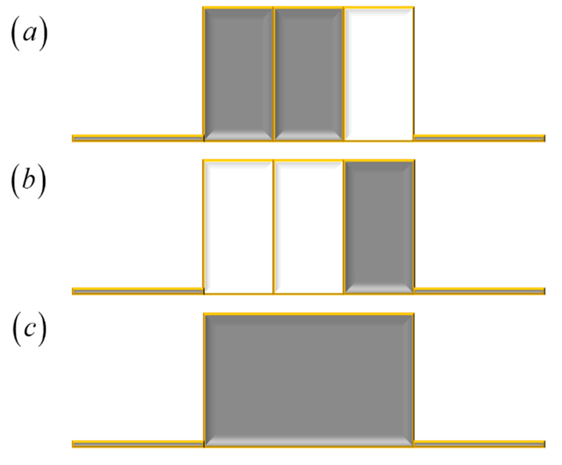
Figure 4.
Pictorial describing the use of Ronchi grating for coding one half of the unit cell, with period d. In (a), at the top, the complementary unit cell of a white and black Barker sequence of length L = 3. At the bottom, the unit cell of a white and black Barker sequence, also of length L = 3. In (b), the optical setup. The complementary grating, at the top of Figure 1 (a), is placed at the input plane. In the absence of a phase gradient, its image covers the grating, depicted at the bottom of Figure 1 (a).
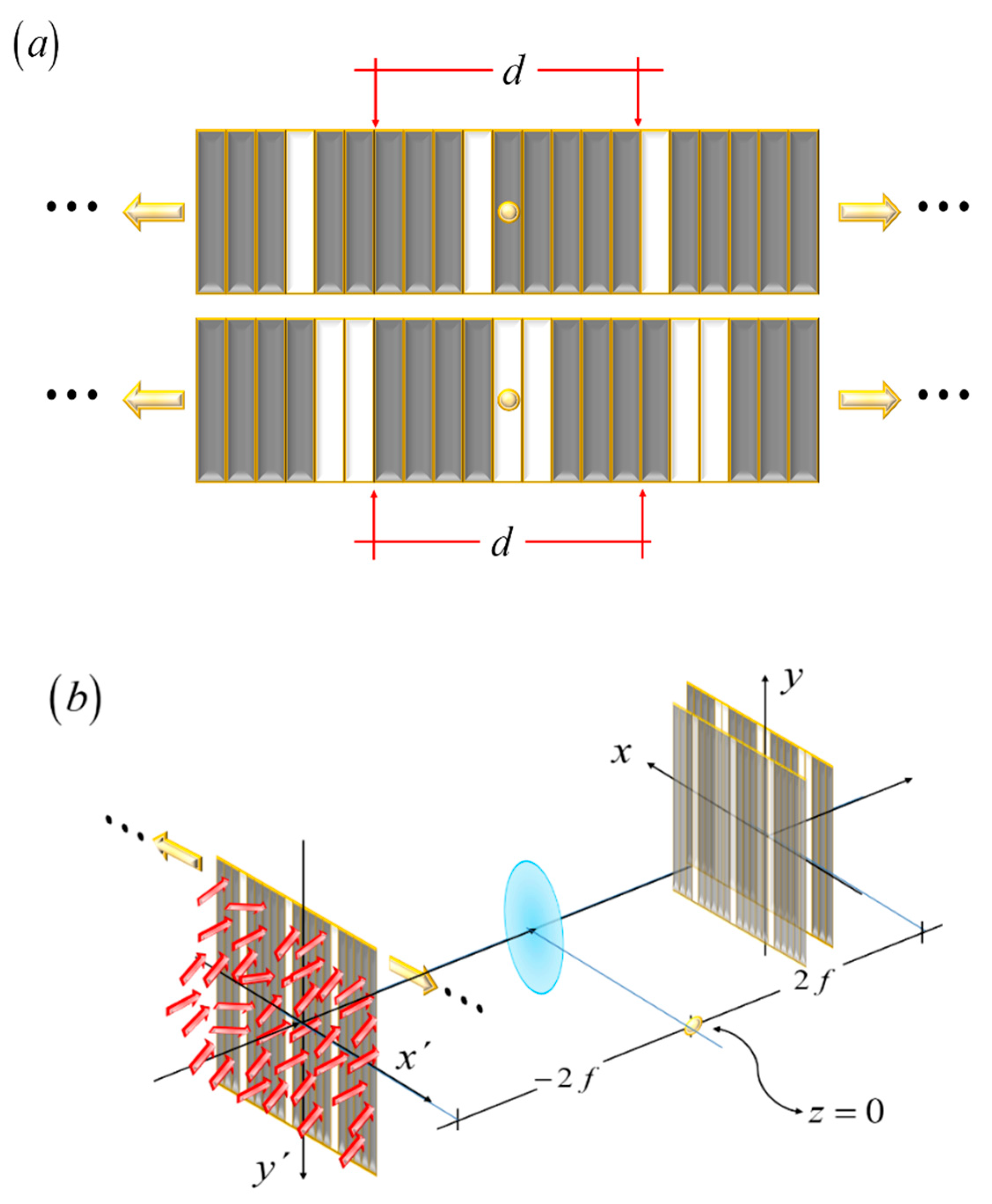
Figure 5.
Cross-Correlations between two complementary gratings. In (a) the length of the sequence is L = 5. In (b), L = 7. In (c), L = 11. In (d), L = 13. And in (e), we plot the cross correlation between two complmentary pseudorandom sequences.
Figure 5.
Cross-Correlations between two complementary gratings. In (a) the length of the sequence is L = 5. In (b), L = 7. In (c), L = 11. In (d), L = 13. And in (e), we plot the cross correlation between two complmentary pseudorandom sequences.
Figure 6.
The optical setup that now includes the presence of a small, randomly located prism at the lens.
Figure 6.
The optical setup that now includes the presence of a small, randomly located prism at the lens.
Figure 7.
The impact of the characteristic function on the cross-correlation of complementary Baker’s masks, with L = 11, and Ω = 0.01. In (a), the deterministic cross-correlation in broken black lines. In red, the deterministic cross-correlation times the square modulus of the characteristic function. In (b) the same as in (a), but for Ω= 0.025. In (c), same as in (a) but for Ω = 0.05.
Figure 8.
A pictorial for presenting a simple description of the Lau effect. In (a), a depiction of the Talbot effect. In (b), the generation of a virtual Fourier spectrum, at the front focal plane of a positive lens. In (c), a line (in red) that links the n-fold diffraction order (at the front focal plane) with the position m d, at the back focal plane.
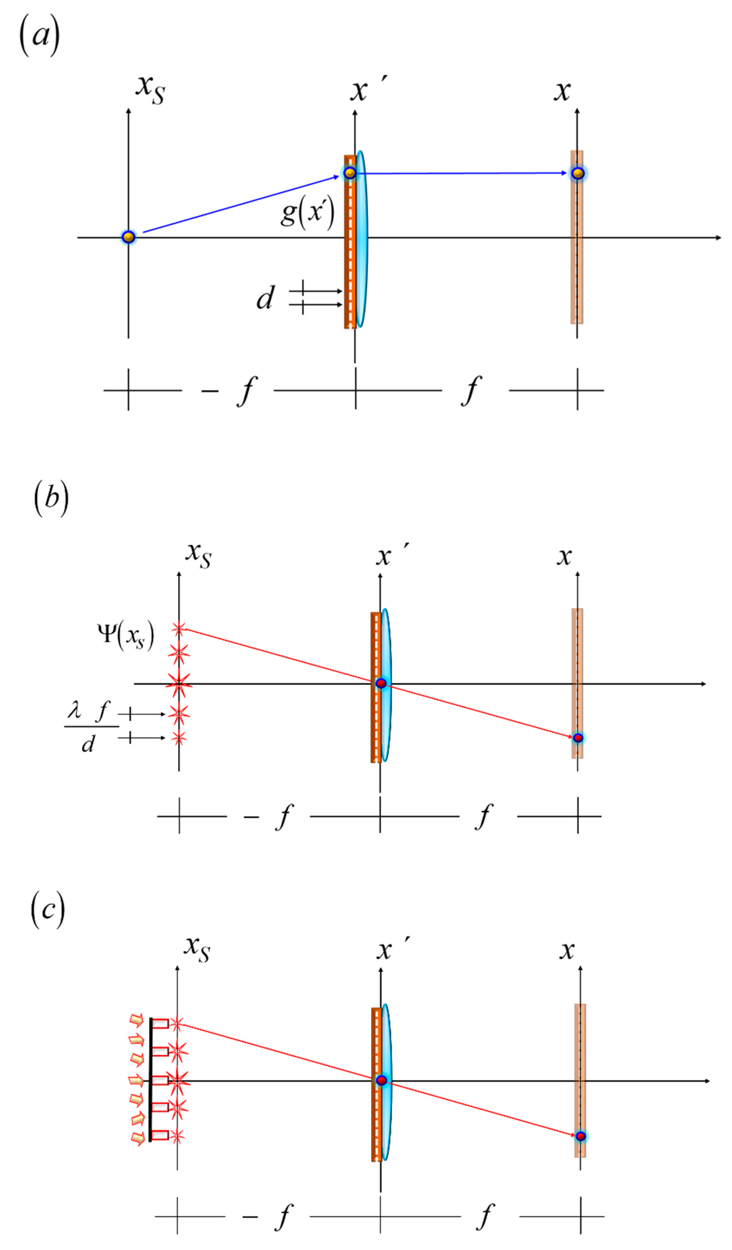
Figure 9.
A folded version of the dark-field, Lau interferometer. In (a), we show an arrangement commonly used in the visualization of fluid dynamics. In (b), we depict a triangular configuration like that used in Sagnac interferometry.
Figure 9.
A folded version of the dark-field, Lau interferometer. In (a), we show an arrangement commonly used in the visualization of fluid dynamics. In (b), we depict a triangular configuration like that used in Sagnac interferometry.
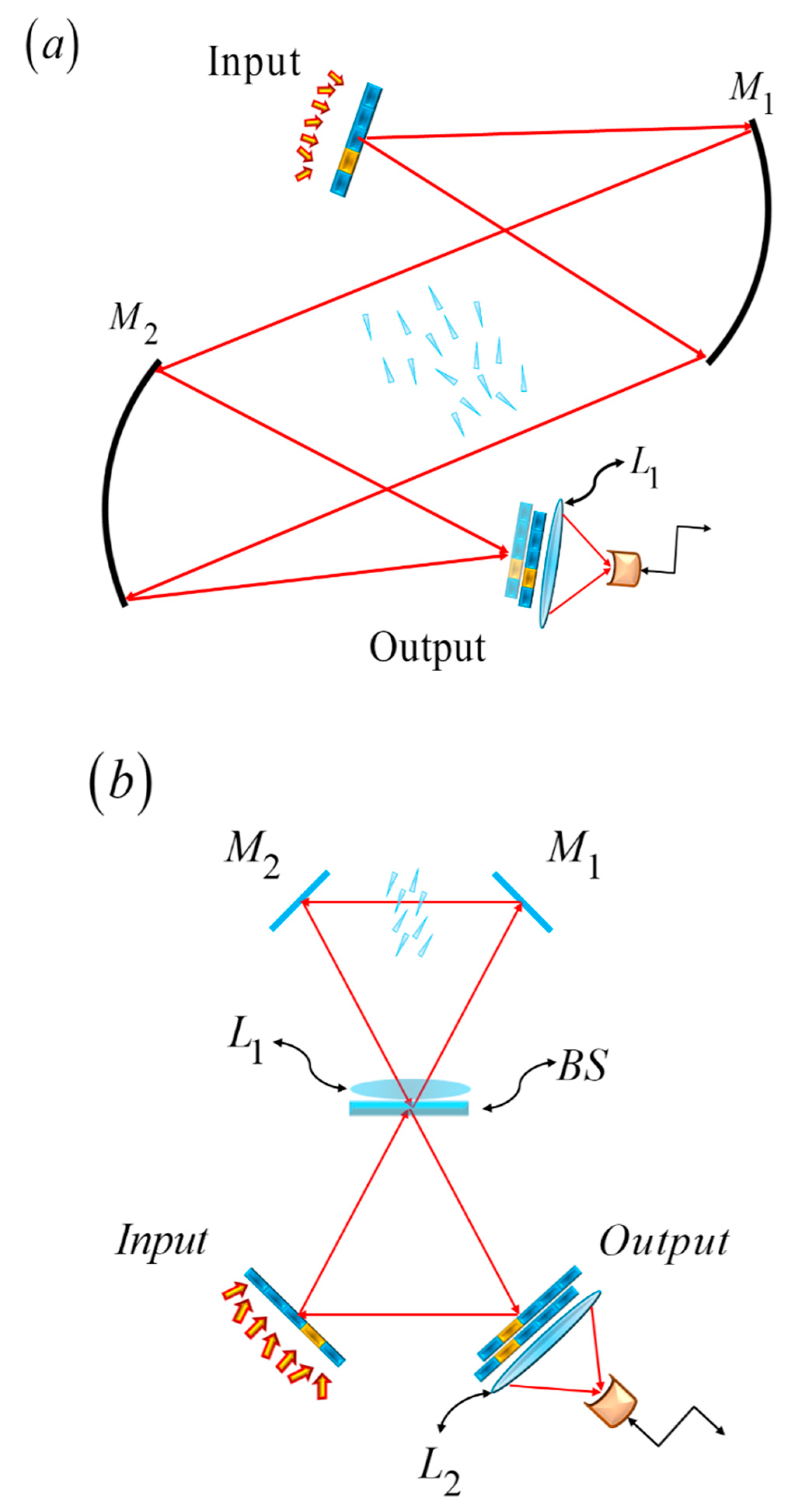

Table 1.
Coefficients, Bn, in Equation (4) associated with the black and white versions of the Barker sequences.
Table 1.
Coefficients, Bn, in Equation (4) associated with the black and white versions of the Barker sequences.
Disclaimer/Publisher’s Note: The statements, opinions and data contained in all publications are solely those of the individual author(s) and contributor(s) and not of MDPI and/or the editor(s). MDPI and/or the editor(s) disclaim responsibility for any injury to people or property resulting from any ideas, methods, instructions or products referred to in the content. |
© 2025 by the authors. Licensee MDPI, Basel, Switzerland. This article is an open access article distributed under the terms and conditions of the Creative Commons Attribution (CC BY) license (http://creativecommons.org/licenses/by/4.0/).
Copyright: This open access article is published under a Creative Commons CC BY 4.0 license, which permit the free download, distribution, and reuse, provided that the author and preprint are cited in any reuse.


