
Submitted:
25 August 2025
Posted:
25 August 2025
You are already at the latest version
Abstract
For designing novel imaging devices, we use masks coded with numerical sequences. These masks work in conjunction with varifocal systems that implement zero-throw tunable magnification. Some masks control field depth, even when the size of the pupil aperture remains fixed. Pairs of vortex masks are used for implementing tunable phase radial profiles, like axicons and lenses. The autocorrelation properties of the Barker sequences are applied to the generation of narrow passband windows on the OTF. For this application, we apply the Barker matrices in rectangular coordinates. A similar procedure, but now in polar coordinates, is useful for sensing in-plane rotations. We implement geometrical transformations by using zero-throw, tunable anamorphic magnifications.
Keywords:
tunable depth of field
; vortex pairs
; passband optical transfer functions
; barker matrices
; angular sensors
; zero-throw tunable anamorphic magnifications
1. Introduction
For several applications in image science, it is important to gather pictures with high resolution and extended depth of field. It is commonly assumed that these two goals are incompatible. For controlling the depth of field of an optical system, the simplest and most commonly use technique consists in reducing the size of the pupil aperture. Of course, this simple solution reduces light gathering power, as well as it decreases the resolution of the optical system. For avoiding this dilemma, here we state the control of firld depth in terms of the OTF [1,2,3,4].
For extending the depth of field with fixed pupil apertures, one can use annular apertures [5,6,7]. This technique has been extrapolated to the use of apertures that are coded with gray level transmittances masks, which have an annular profile over the whole pupil aperture [8].
By taking into account the image quality chain, as in Figure 1, some of us have suggested a different approach. In a previous proposal, we consider gathering high qualty 3-D images, in a single-snapshot. To this end we employ a two stage process. In the first stage,the optical system employs a mask (in generic terms an apodizer) that reduces the impact of focus error [9]. In other word, the optical system performs a pre-processing operation. By reducing the influence to focus errors, the pre-processing masks collects with the same image quality, all the planes contained in the 3-D image. The same image quality means that the OTF does not have zero values even when one changes the focus error coefficient. This property has a price. The recorded images have a reduction in signal modulation. And hence, the recorded picture is not necessarily suitable for human visualization. However, the single snapshot can be used to compensate the reduction of signal modulation. For this latter task, it is desirable to use a simple, digital post-processing algorithm.
For achieving our inteded aim, it is convenient to recognize that the mask must generate optical system a modulation transfer function (MTF) with the two following characteristics: a) In the absence of noise, the MTF should be different from zero within its passband of the optical system. b) In the presence of noise, the values of the MTF should be equal to or greater than a given threshold value, for surpassing the variations of white noise [10].
In parallel to these developments, we note the need for having optical systems with tunable magnification. Typically, one associates variable magnifications with the use of zoom systems, or with the use of varifocal lenses. According to Plummer, Baker, and van Tassell [11], it was Kitajima [12] who filled the first patent of varifocal lenses. Kitajima´s proposal was improved with the innovations of Lohmann [13,14,15,16] and of Alvarez [17,18]. In the last decade, several technological developments have been achieved for implementing lenses with tunable optical power [19,20,21,22,23,24,25,26,27,28]. Then, as natural step, we incorporate the use of varifocals systems for proposing novel optical devices.
Our current aim is to propose new optical systems that incorporate masks coded with numerical sequences, The masks can work in conjunction with varifocal systems [29,30]. In this publication we discuss optical systems with tunable magnification at zero-throw [31,32].
In section 2, we discuss optical methods for extending the depth of field. We emphasize on a generalized version of the Lohmann-Alvarez technique for controlling the optical path difference in transparent masks. This generalizatio allow us to propose optical devices that govern field depth while preserving the same full pupil aperture. In section 3, we exploit the autocorrelation properties of the Barker sequences [33], in rectangular coordinates, for generating narrow pass windows on the OTF. In section 4, we apply the Barker sequences, in polar coordinates, for proposing an optical sensor of in-plane rotations [34]. In section 5, we consider the use of zero-throw tunable anamorphic magnifications for performing geometrical transformations [35,36,37]. And in section 6, we summarize our contribution.
2.1. Multiple Snapshots: an Average OTF
In approach was advanced by Haeusler, who proposed to record (on the same photographic plate) several out-of-focus images of the same object. In this manner, one can generate an averaged OTF, which alleviates the impact of focus errors [38].
For avoiding errors due to misalignments and to magnification variations, one of us proposed an alternative method. As depicted in Figure 1, for this technique, the detection plane remains fixed, while one records a finite number of snapshots. At each snapshot, the optical system varies the focus error coefficient. This technique overcomes the limitations imposed by the detector dynamic range [39]. In what follows, we discuss a simple model for the latter technique.
For a 1-D imaging process, the out-of-focus OTF reads
In Equation (1) we denote the spatial frequency with the Greek letter μ. At the edge of the pupil aperture, the cutoff spatial frequency is Ω. As is common in scalar diffraction, the wavelength is denoted as λ. The in-focus OTF is
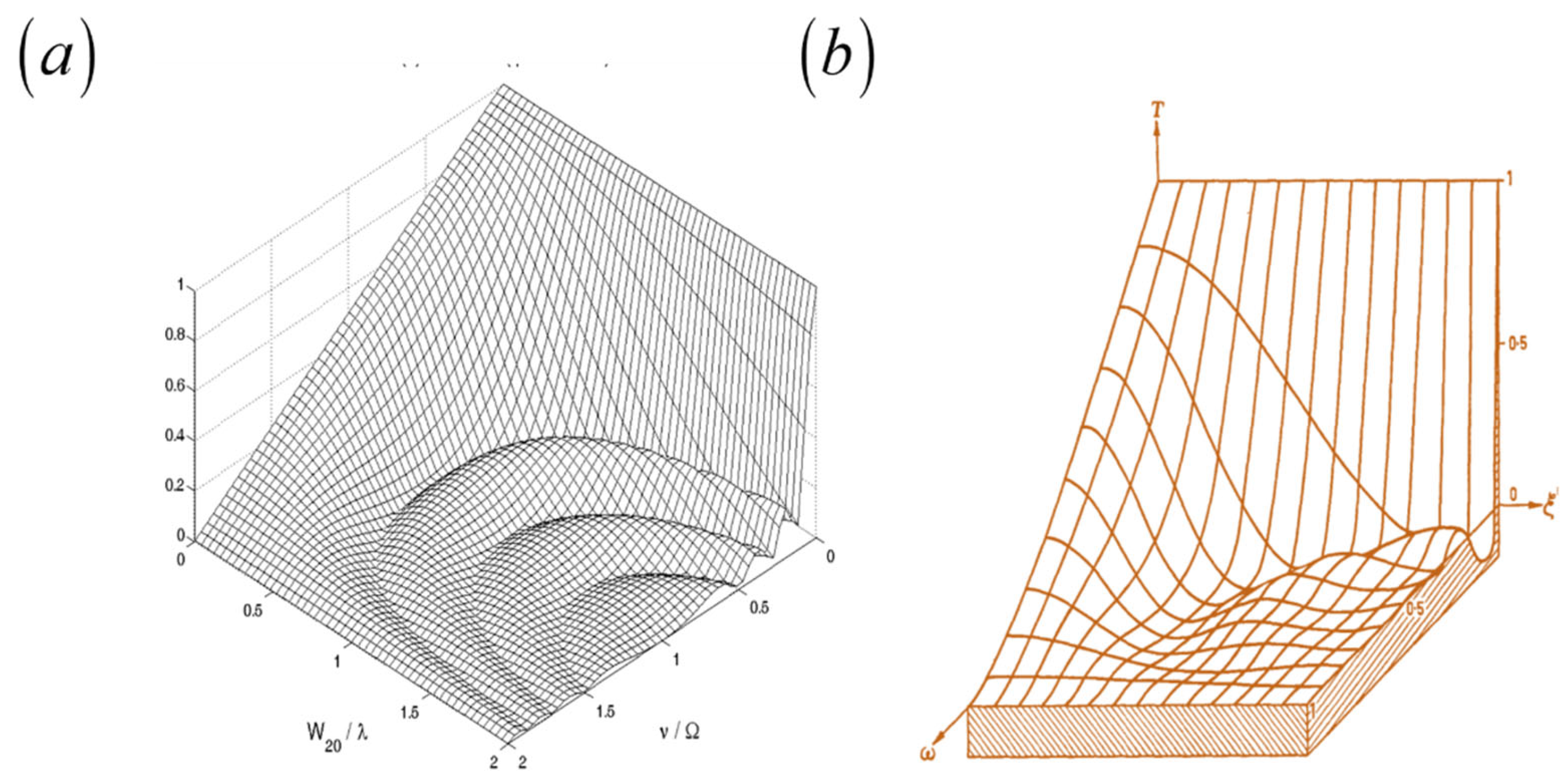
In Figure 2, we show 3-D graphs of the OTF in Equation (1).
Figure 2.
Optical system for tuning the focus error coefficient, while the image is recorded at a fixed position. In (a), a pictorial describing Hauesler´s proposal. In (b), the optical setup is now an optical processor, which has a varifocal field lens, at the Fourier domain. We assume that the pupil aperture has a rectangular shape. In (c), the representation shows that the field lens do not alters the magnification, M = -1, evenwhen the image position moves along the optical axis.
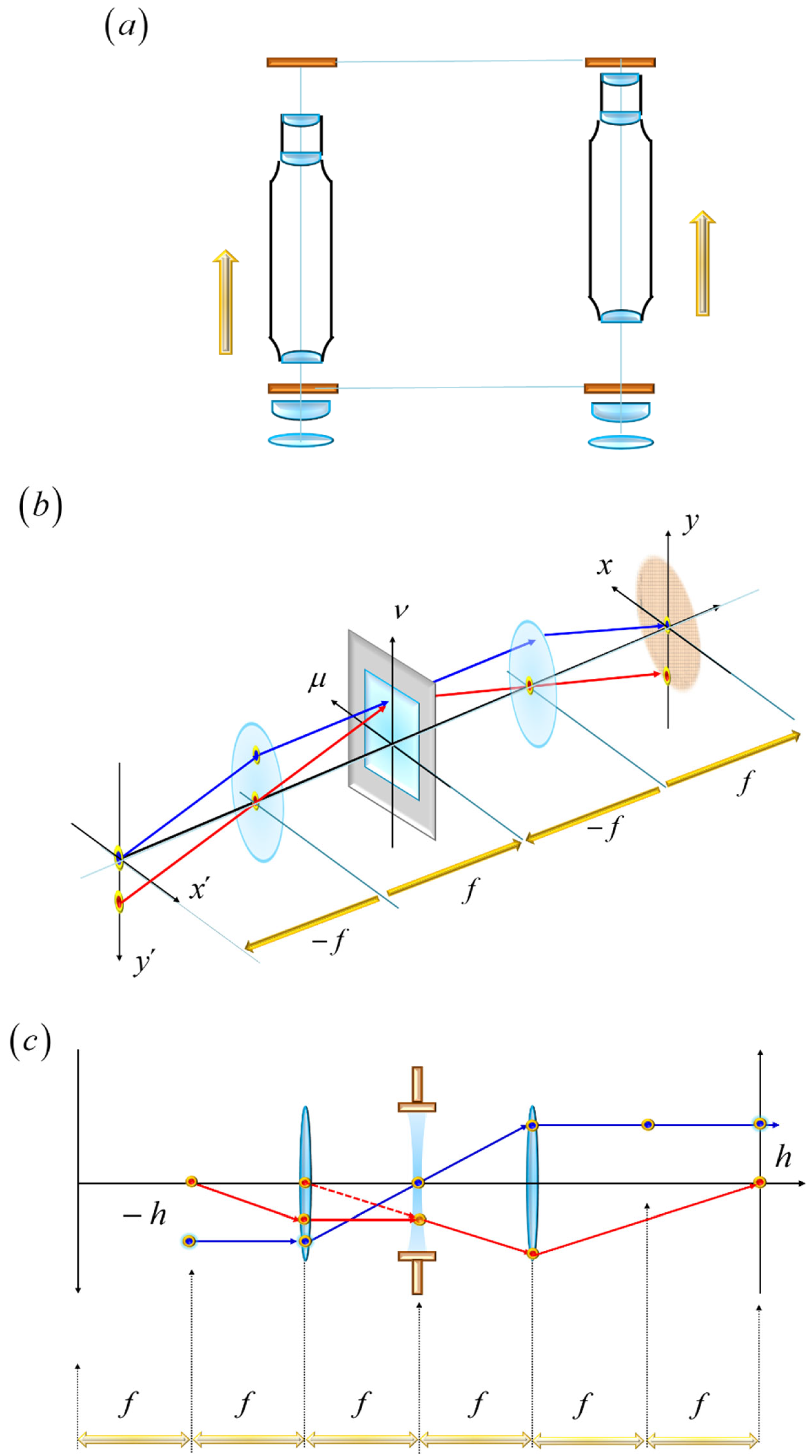
Figure 3.
The influence of focus error on the OTF, as in Equation (1). In (a), the variations of the focus error coefficient is in the interval (0, 2 λ). In (b), we show the first numerical evaluations, as reported by Steel.
Figure 3.
The influence of focus error on the OTF, as in Equation (1). In (a), the variations of the focus error coefficient is in the interval (0, 2 λ). In (b), we show the first numerical evaluations, as reported by Steel.
Next, we consider that one records several snapshots, say N. At each snapshot one changes the optical power of the field lens, then one can the focus error coefficient. That is, at n-fold snapshot the focus error coefficient is W2,0. = Wn, where Wn can be either a deterministic value, or a random real number. We define the average OTF as
In Equation (3) we include a weighting factor, pn, which one can incorporate digitally at each snapshot. The weighting factors can be arbitrarily selected. And if there are positive real numbers, with values less than unity, the weighting factors can be thought of as probability values taken from density function. By substituting Equation (1) in Equation (3), we obtain
From Equation (4), we note that the average OTF can resemble the in-focus OTF. In Figure 2, we show a numerical simulation that shows the impact of the second factor in Equation (4).
Figure 4.
Graphs of the OTF for some deterministic values of the focus error coefficient. The number of snapshots is N = 4. For any n, the value of the weighting factor is pn = 1/16. In blue lines the in-focus OTF. In red lines the average OTF. In (a), the focus error coefficient varies from λ/4 until λ, in steps of λ/4. In (b), the focus error coefficient varies from λ until 4 λ, in steps of λ. In this latter case the average OTF can have negative values.
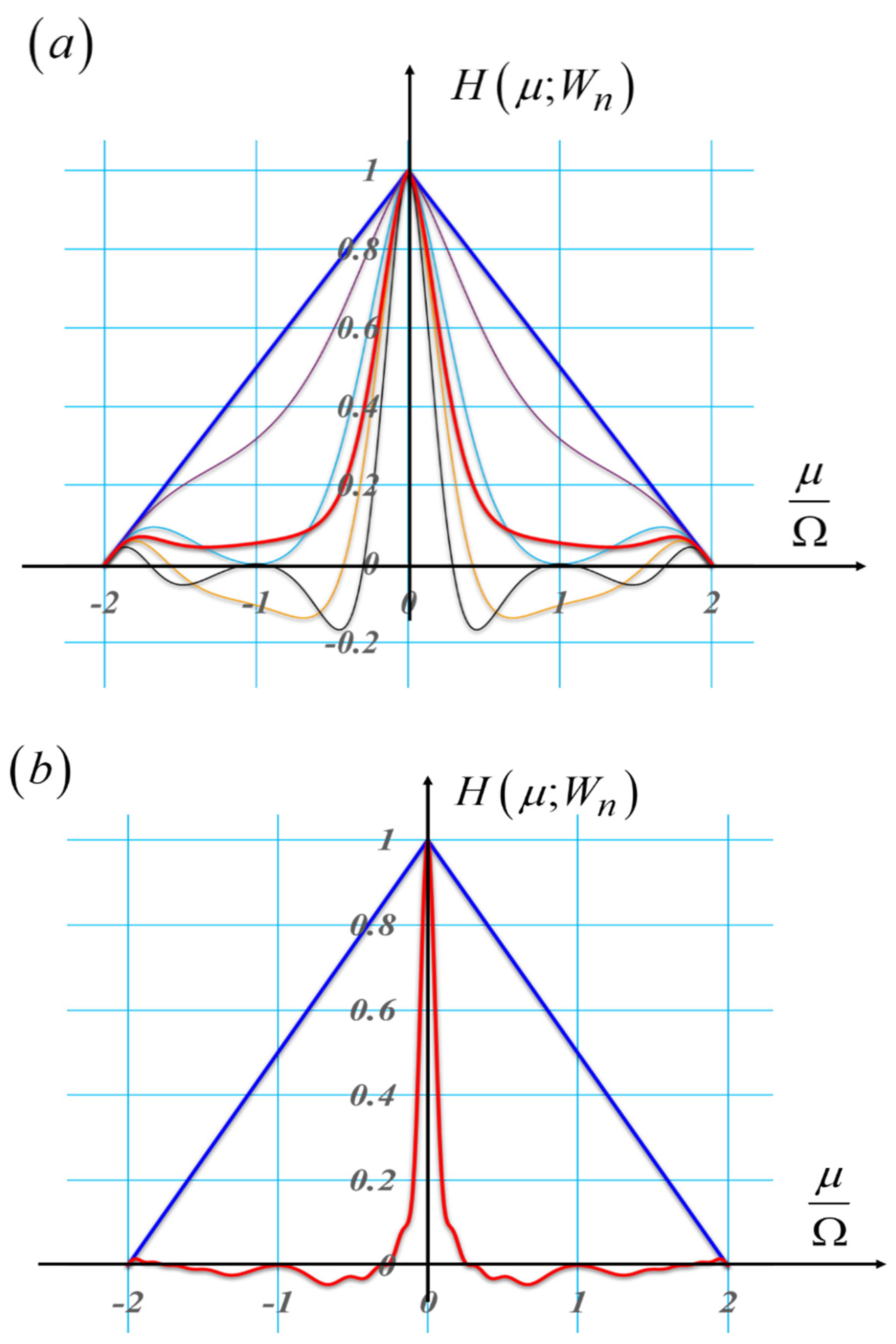
Figure 5.
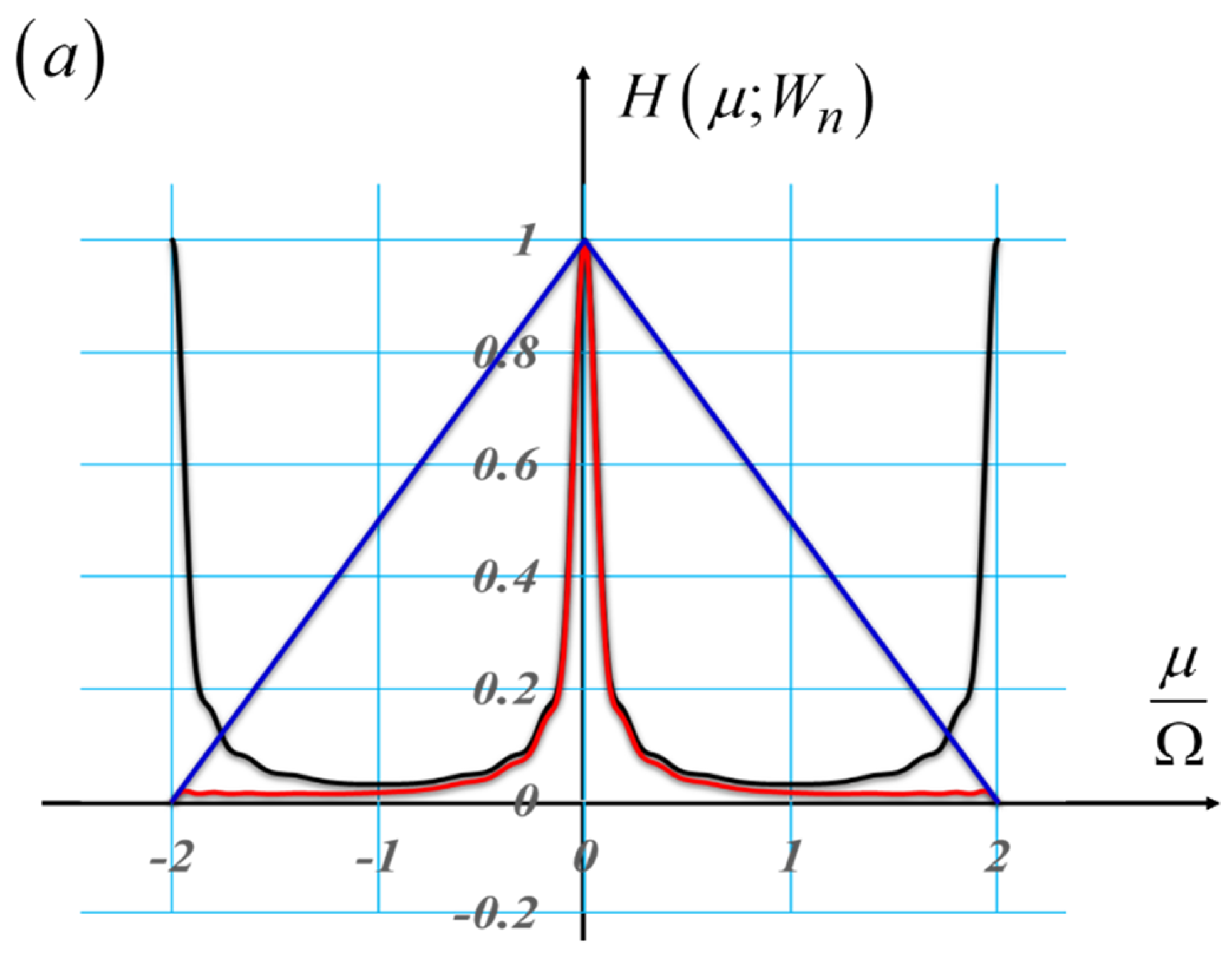
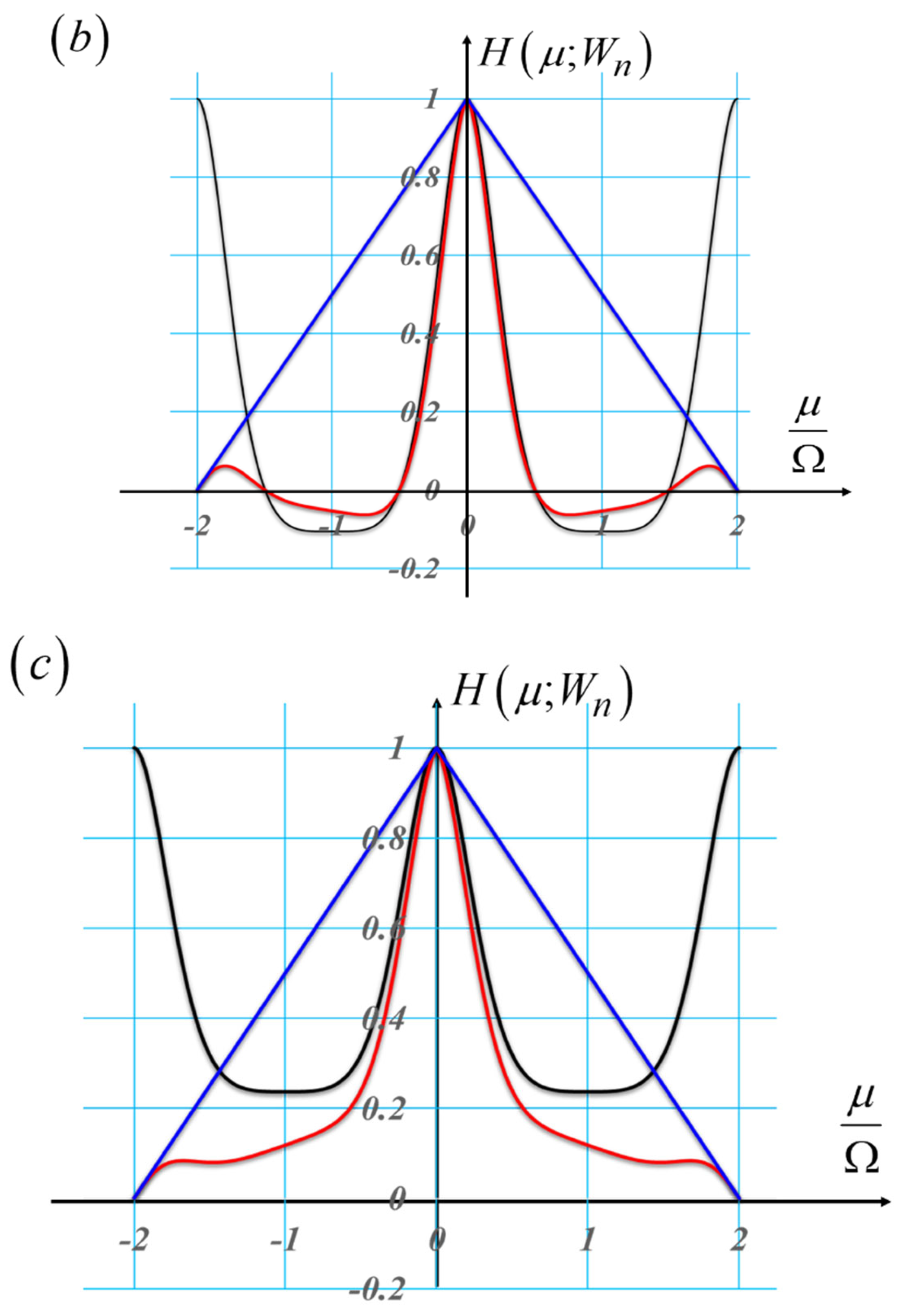
Graphs obtained if the focus error coefficient is randomly selected inside the interval (- λ, λ). We assume that the probability density function obeys the uniform distribution with zero mean. In blue lines the in-focus OTF. In red lines the average OTF. In black lines the second factor in Equation (4). Due to the random variations, we note the following. In (a), the average OTF has only positive values. In (b), we show that the average OTF can have negative values. In (c), the average OTF has values that are greater than the values in (a).
Figure 5.
Graphs obtained if the focus error coefficient is randomly selected inside the interval (- λ, λ). We assume that the probability density function obeys the uniform distribution with zero mean. In blue lines the in-focus OTF. In red lines the average OTF. In black lines the second factor in Equation (4). Due to the random variations, we note the following. In (a), the average OTF has only positive values. In (b), we show that the average OTF can have negative values. In (c), the average OTF has values that are greater than the values in (a).
2.2. Single Snapshot: A Useful Similarity.
Searching for useful tools for describing the imaging process, in terms of scalar diffraction, Papoulis [40], Guigay [41] and Goodman [42] propose the use of the ambiguity function in optics. Some of us noted that there is indeed a mathematical similarity between the expression for the out-focus OTF and the expression for evaluating the ambiguity function. That is, the integral for evaluating the out-focus OTF reads
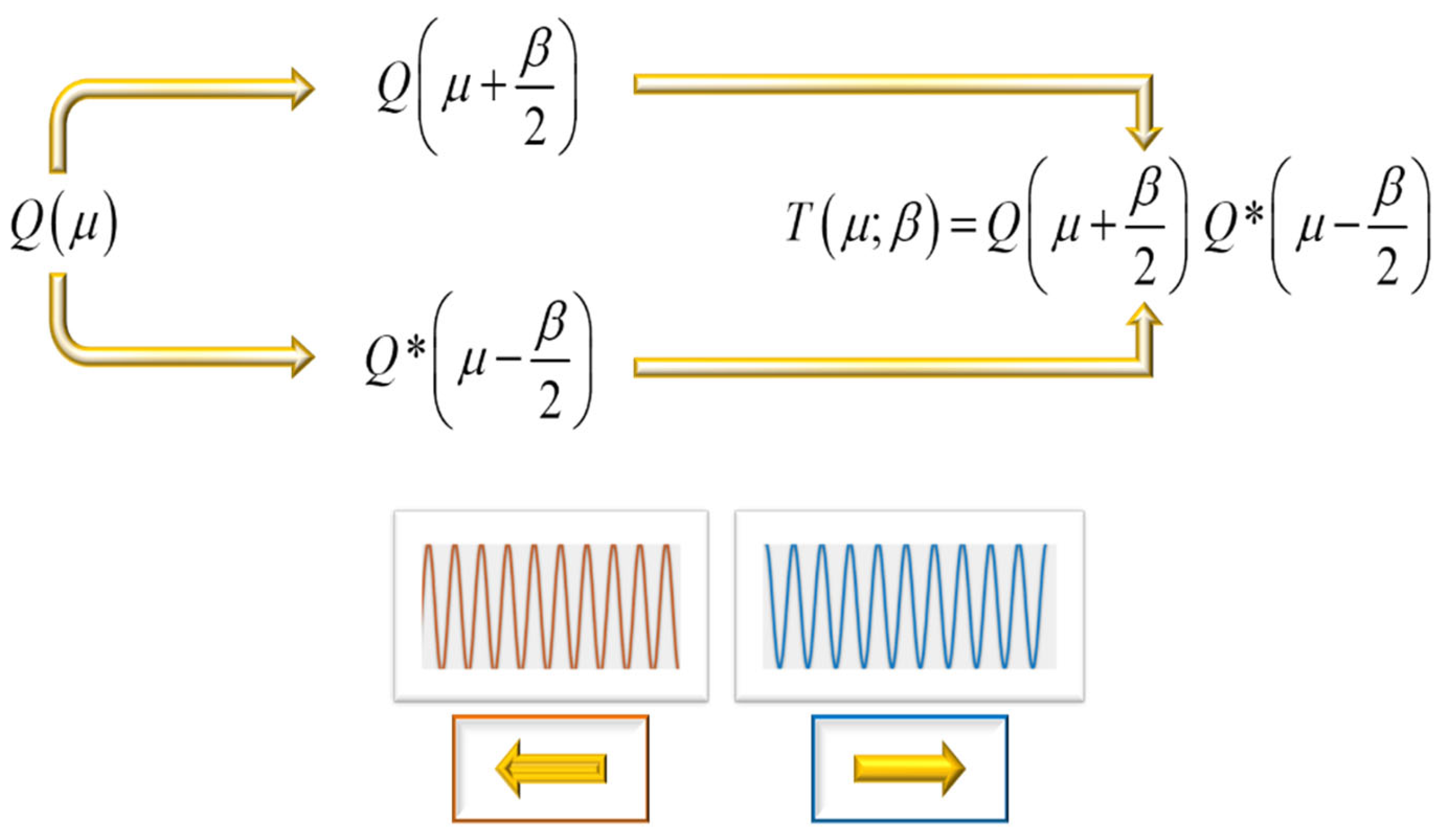
This analogy was applied for linking the visualization of the ambiguity function with a nonconventional display of the out-of-focus OTF [43]. To this end, as shown in Figure 6, we recognize the following relationships
In Equation (7) we change the temporal frequency ν by the spatial frequency µ, and the temporal variation, t, into a spatial variation, y. And then we recognize that the spatial variation is related linearly with the spatial frequency µ. The slope of the linear relationship is proportional to the focus error coefficient W2,0. For obtaining a value of the MTF, with focus error, one traces a straight line through the origin with slope 2 W2,0 / (λ Ω2). Next, we find the intersection of this inclined line with a vertical line located at µ = σ. The point (σ, 2 W2,0 / (λ Ω2)) indicates visually the out-of-focus MTF H(σ, W2,0). Hence, one can argue that the modulus of the ambiguity function is a highly redundant picture since it contains all the defocused MTFs.
The picture in Figure 6 (a) indicate visually that the ambiguity function of a clear pupil aperture changes substantially with an in-plane rotation. While the picture in Figure 6 (b) changes slowly with an in-plain rotation. Of course, this heuristic description should be part of a 3-D display of the MTFs as in Figure 7.
The results in Figure 7 were obtained with masks that can change their optical path difference [44]. In what follows we indicate how it is possible to modify the optical path difference. The above description has been considered by several other authors, who have pointed out the strengths and the limitations of our initial proposal [45,46,47,48,49,50,51,52].
2.3. Generalized Lohmann-Alvarez Pairs
In remarkable contributions, Lohmann and Alvarez proposed the use of two phase conjugated, cubic phase masks for implementing a varifocal lens. In mathematical terms, their procedure reads as follows
In Equation (8), we follow the same notation as in Equation (1). But now, the lower-case letter “a” denotes the optical path difference (in units of λ) of the cubic phase mask. If one uses a pair of phase conjugate masks that are laterally shifted, say by the spatial frequency β, then the complex amplitude transmittance is
By substituting Equation (8) in Equation (9) one obtains
From Equation (10), we observe that the second term has a quadratic phase variation that can be thought of as the complex amplitude transmittance of lens. As the optical path difference changes with the lateral shift beta, then the lens has variable focal length. It is relevant to note that the mathematical steps for going from Equation (8) to Equation (10) can be associated with the procedure used in the calculus of differences [53]. Therefore, as a working hypothesis, we want to explore other possibilities. As depicted in Figure 7, we show the steps for obtaining a generalized version of Lohmann-Alvarez technique.
Figure 8.
Generalized Lohmann-Alvarez phase conjugate pairs. We use the calculus of differences, on phase delays, for generating tunable 1-D optical path differences.
Figure 8.
Generalized Lohmann-Alvarez phase conjugate pairs. We use the calculus of differences, on phase delays, for generating tunable 1-D optical path differences.
We discuss two cases. In the first case, we describe a technique for controlling the diffraction efficiency of a sinusoidal phase grating [54]. In the second case, we discuss a similar technique for tuning the optical path difference of a mask that extends the depth of field [55]. And consequently, it opens the possibility of governing the depth of field, at full pupil apertures. For the first case, we consider the complex amplitude transmittance
In Equation (11), the Greek letter η denotes the period of the phase grating if one uses spatial frequencies. That is, η = d /λ f. Now, if one uses a phase conjugate pair, the complex amplitude reads,
By substituting Equation (11) in Equation (12), we have that
In Equation (13) the new optical path difference is expressed as an amplification equation
It is clear from Equation (14), and from Figure 9, that one can control the amplification associated with the amplitude of the sinusoidal phase variation, by a lateral displacement of the elements forming the phase conjugate pair.
For the sake of completeness in our current discussion, in Figure 10, we show some steps associated with the proposed procedure.
For the second case, of the above proposed generalization, we consider the use of a pair of masks, which have hyperbolic phase varitions. In this case, for the intial mask, the complex ampltude transmittance reads
We use Equation(15) for setting a pair. The elements of the pair are laterally shifted by the spatial frequency β. Then, the complex amplitude distribution is
By substituting Equation (15) in Equation (16) we obtain
In Equation (17) the upper-case letter A denotes the amplification obtained by using the pair. That is,
At the left-hand side of Figure 11, we plot the phase profiles of the hyperbolic masks under discussion. In blue the variations are associated with the even function of a hyperbolic cosine. In red the variations that are associated with the odd function of a hyperbolic cosine. At the right-hand side of Figure 11, we plot the amplification ratio as a function of the lateral displacement β.
For the sake of completeness in our current discussion, in Figure 12, we show some steps associated with the proposed procedure.
We discuss now the MTFs associated with the use of the masks with hyperbolic phase profiles, which can tune the optical path difference by a lateral shift between the masks. In Figure 13 (a), as reference, we show the impact of focus errors on the MTF of a clear pupil aperture. The focus error coefficient varies from W2,0 = 0 until W2,0 = 3 λ, in steps of λ. In Figure 13 (b), we show the impact of focus errors on the MTF of a mask with that uses a pair hyperbolic phase profile, as in Equation (17). Again, the focus error coefficient varies from W2,0 = 0 until W2,0 = 3 λ, in steps of λ.
It is apparent from Figure 13 (b) that the MTFs are practically the same, for variations of the focus error coefficient in the range |W2,0| < 3 λ, provided that the amplitude of the hyperbolic variations have an optical path difference a = 17 λ. Hence, one can tune the depth of field by shifting laterally the elements of the hyperbolic pair. In next section, we show that the above results can be translated to the control of the optical path difference, but now in polar coordinates.
2.4. A Vortex (Helical) Pair
In Figure 14, we show the steps for obtaining an angular version of the Lohmann-Alvarez technique. Instead of a lateral displacement between the members of the pair, now we consider that the elements are in plane rotated by an angle β.
For this application, we consider that the initial mask has a vortex complex amplitude transmittance
Next, we form a pair by placing together one element and its complex conjugate element. The forming elements are in-plane rotated by an angle β. In mathematical terms,
By substituting Equation (19) in Equation (20) we obtain the overall complex amplitude transmittance
It is clear from Equation (21) that by selecting a linear phase variation, R(ρ) = (ρ/Ω,) we can control the optical path difference of an axicon. Furthermore, by selecting a quadratic phase variation, R(ρ) = (ρ/Ω)2, we can govern the optical path difference of a lens. Trivially, the same procedure applies for higher order terms. And in this manner, we can control the magnitude of the aberration coefficients of a given wavefront.
In Figure 15, we exhibit a pictorial that displays the results in Equations (13), (17) and (21). The pictorial summarizes our goal for extending the Lohmann-Alvarez technique of using pairs of masks for controlling the optical path difference.
In the next section, we focus our attention to the use of masks that are coded with the Barker sequences.
3. Narrow Passband Windows: Rectangular Barker Matrices
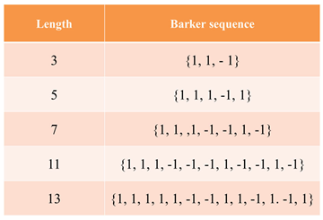
In this application, we employ masks that are coded with the Barker sequences, which are listed in Table 1.
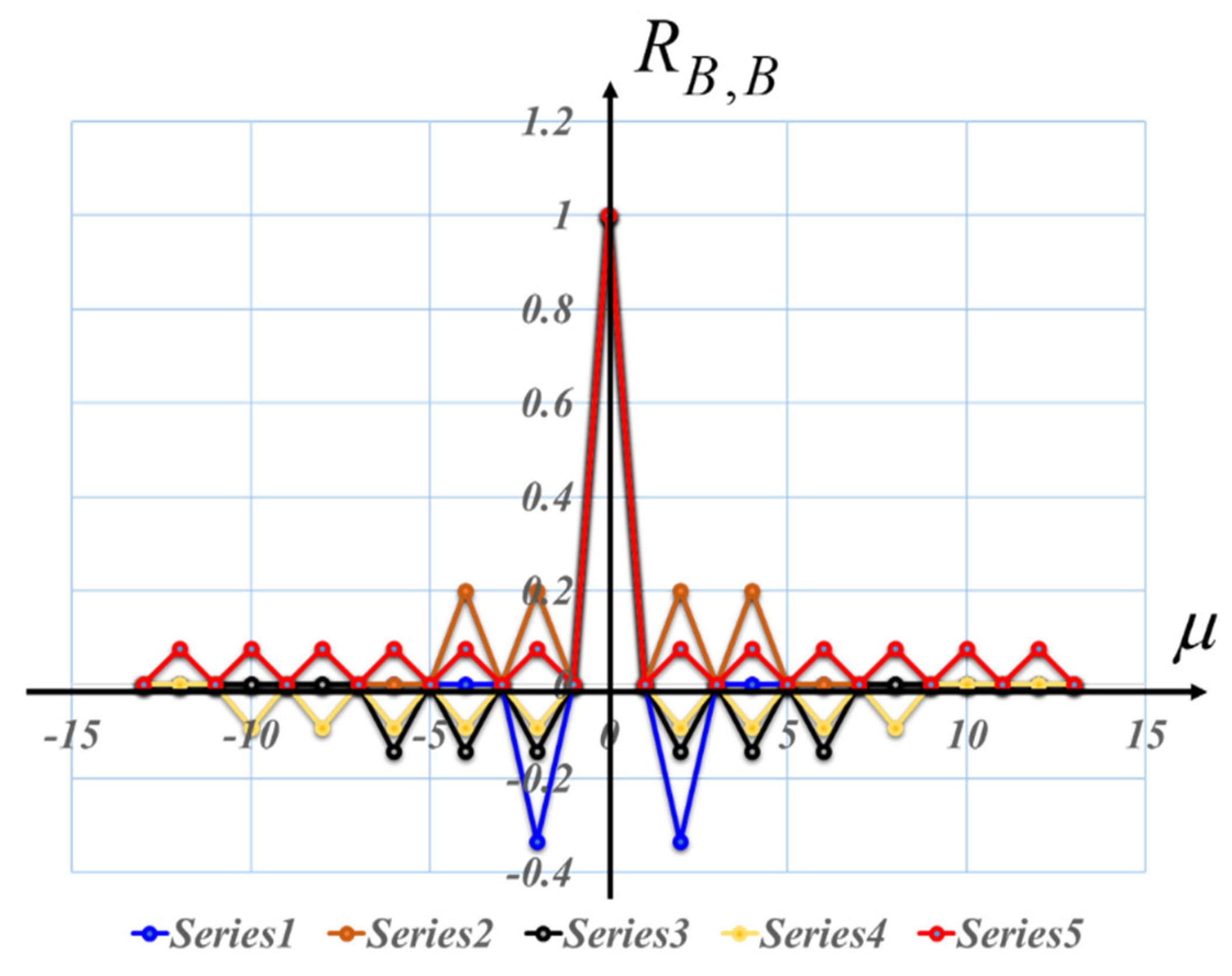
A remarkable feature of the Barker sequences are their autocorrelations, which consist of a distinctive, narrow central peak. Around the main peak, there are secondary peaks with low amplitude. Now, the OTF is the autocorrelation of the pupil function. If the pupil is coded with a Barker sequence, then the associated OTF inherits the autocorrelation characteristics of Barker sequences.
Figure 16.
Graph showing the autocorrelations of the Barker sequences that are listed in Table 1.
Figure 16.
Graph showing the autocorrelations of the Barker sequences that are listed in Table 1.
It is known that two narrow slits can be suitably employed for obtaining windows on the OTF in Moiré photography [56,57,58,59]. Now, the OTF is the autocorrelation of the pupil function. Hence, as depicted in Figure 17, if the pupil is coded with a Barker sequence, then the associated OTF inherits the autocorrelation characteristics of Barker sequences. And in this manner, we generate narrow windows on the OTF.
In Figure 18, we illustrate the coding of the pupil aperture with a pair of Barker masks, in substitution of the narrow slits. For implementing this idea in two dimensions, it is necessary to extend the concept of coded sequences in matrix format.
In Figure 19, we show the Barker matrices of order n X n, when n = 3, 5, 7, 11, and 13.
In the above application, the extension to the Barker matrices is done in rectangular coordinates. It is also possible to define the Barker matrices in polar coordinates, as we discuss next.
4. Rotational Sensor: Radial Barker Matrices
In Figure 20, we show the scheme for obtaining spokes that are coded angularly with the Barker sequences. At the left-hand side of Figure 20, we depict the angular coding of the Barker sequence of length L = 13. For some applications, it may be necessary to have more than 13 radial slits. If this is the case, at the right-hand side of Figure 20 we show a mask that contains 169 radial slits. In this latter case, the code is direct product of the Barker sequence of length 13; as is discussed in [60].
The above-described masks were employed for setting a sensor of in-plane rotations. For this application, the optical setup is shown in Figure 21.
We note that the coding scheme in Figure 20 and Figure 21 are restricted to angular variations. So, the following question arises. Is it possible to implement the coding in radial and angular variations? The answer to the question is yes. In Figure 22, we show masks that code the previous Barker matrices, but now in polar coordinates. In fact, for that mask in Figure 22, the radial variation is quadratic as is common in zone plates. Therefore, the masks in Figure 22 are zone plates that are coded with the Barker sequences.
As part of our current scope, in the following section, we include the use of varifocal systems, which can work in conjunction with the already discussed masks.
5. Tunable Anamorphic Magnifications
In Figure 23, we show an optical setup that generates variable magnification between to conjugate planes, which are separated by a fixed distance, T, known as the throw.
From Figure 23, we observe that it is necessary to employ at least two varifocal lenses for achieving tunable magnifications, while preserving the axial positions of the conjugate planes. In Figure 23 (a), we indicate the need to perform two actions for implementing tunable magnifications with fixed throw, T. As the optical power of the lens changes, one needs to move the varifocal lens along the optical axis. In (b), we show the use of two varifocals for implementing tunable magnification of the input picture, while preserving the image at the input plane. The varifocal system is a zero-throw device. In Figure 23 (c) we employ an initial collimating lens, which has fixed optical power. At its back focal plane, we can implement an angular tunable magnification, by using two varifocal lenses. In this manner this device is a Barlow lens that preserves the location of the initial back focal plane, while tuning the angular magnification [58].
Furthermore, we have noted that optical system in Figure 23 (b) can be used to generate tunable anamorphic magnifications [59]. To this end, we substitute the varifocal spherical lenses by varifocal cylindrical lenses as is depicted in Figure 25.
Furthermore, we have noted that optical system in Figure 23 (b) can be used to generate tunable anamorphic magnifications [59]. To this end, we substitute the varifocal spherical lenses by varifocal cylindrical lenses as is depicted in Figure 25.
Figure 24.
Optical setup that uses two pairs of cylindrical varifocal lenses for tuning (with zero-throw) the magnification in an anamorphic fashion.
Figure 24.
Optical setup that uses two pairs of cylindrical varifocal lenses for tuning (with zero-throw) the magnification in an anamorphic fashion.
A nonconventional application of the tunable anamorphic magnification is the production of geometrical transformations, which were pioneered by Bryngdahl. For illustrating this application, we show the optical setup in Figure 25.
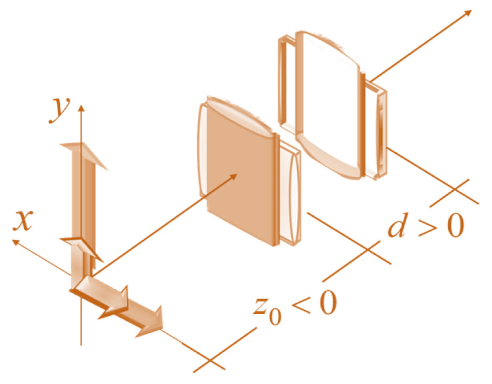
Figure 25.
Schematics of an optical setup that emplos the lenses in Figure 23. In (a),along the x-axis the magnification M = -1. In (b), along the y-axis the absolute valu of the magnification is greater than unity.
Figure 25.
Schematics of an optical setup that emplos the lenses in Figure 23. In (a),along the x-axis the magnification M = -1. In (b), along the y-axis the absolute valu of the magnification is greater than unity.
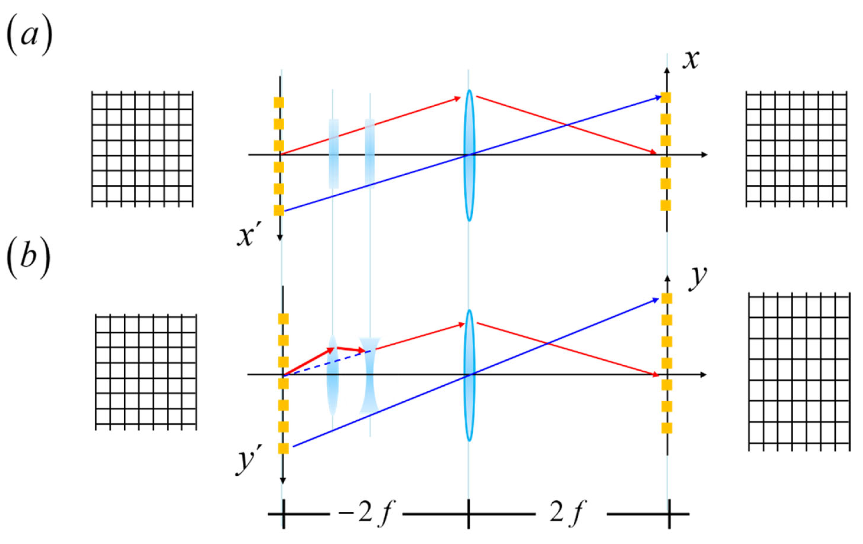
In Figure 26 we show some numerical simulations of the proposed geometrical transformations. In Figure 26 (a), the image of a baboon has the same magnification along the x-axis and the y-axis. In Figure 26 (b), the absolute value of the magnification along the x-axis is higher than that along the y-axis. And in Figure 26 (c), the absolute value of the magnification along the x-axis is smaller than the absolute value of the magnification along the y-axis.
At this stage, except for the use of anamorphic spectacles, we do not have other applications for tunable, anamorphic magnifications.
6. Final Remarks
We have applied some numerical sequences for coding masks, which are used in conjunction with varifocal systems for designing novel imaging devices. Specifically, we have exploited the concept of average OTF for extending the depth of field of an optical system. Furthermore, we have extended the Lohmann-Alvarez technique (in rectangular coordinates) field depth, while preserving the size of the pupil aperture. For this application, we have discussed the use of the calculus of differences in the design of devices with governable optical path differences.
We have noted that there is an analogy between the Lohmann-Alvarez technique rectangular coordinates, and the use of a pair of vortex lenses in polar coordinates. We have exploited this analogy for designing optical pairs of vortex masks, which can generate tunable phase radial profiles, like axicons and lenses.
We have exploded the autocorrelation properties of the Barker sequences for generating narrow passband windows, on the OTF. For applications in 2-D Moiré photography, we discussed the use of rectangular masks, which are denoted as the Barker matrices.
A similar procedure, but now in polar coordinates, is useful for designing novel zone plates, here denoted as Barker zone plates, for sensing angular shifts.
We have explored the use of optical systems that generate tunable magnification at zero-throw, for describing anamorphic tunable magnifications, which are of interest in optical processors that produce geometrical transformations.
Acknowledgements
We express our most sincere gratitude to the International Commission for Optics (ICO) for honoring us with the Galileo Galilei Medal. We are also truly indebted to Prof. Manuel Filipe Costa for his cordial invitation to present this contribution, as an invited paper in the AOP Conference in Aveiro, Portugal. And happily, we extend our gratitude to several of our previous co-authors and students, who helped us to obtain the many results reported here. Special thanks go to Professor Pedro Andrés Bou and to Prof. Amparo Pons Marti for their good-natured friendship.
Conflicts of Interest
The authors declare that there are no conflicts of interest related to this article.
References
- Duffieux, P.M., L’integrale de Fourier et ses applications à l’optique (Besançon, 1945).
- Hopkins, H.H. The frequency response of a defocused optical system. Proc. Phys. Soc. 1955, 231, 91–103. [Google Scholar]
- Steel, W.H. The defocused image of sinusoidal gratings. Optica Acta 1956, 3, 65–74. [Google Scholar] [CrossRef]
- Mino, M.; Okano, Y. Improvement in the OTF of a defocused optical system through the use of shaded apertures. Appl. Opt. 1971, 10, 2219–2225. [Google Scholar] [CrossRef]
- Welford, W.T. Use of annular apertures to increase focal depth. J. Opt. Soc. Am. 1960, 50, 749–753. [Google Scholar] [CrossRef]
- Tschunko, H.F.A. Imaging performance of annular apertures. 3: Apodization and modulation transfer functions. Appl. Opt. 1979, 18, 3770–3774. [Google Scholar] [CrossRef]
- Mahajan, V.N. , José Antonio Díaz. Imaging characteristics of Zernike and annular polynomial aberrations. Applied Optics 2013, 52, 2062–2074. [Google Scholar] [CrossRef]
- Ojeda-Castañeda, J.; Valdos, L.R.B.; Montes, E.; Ojeda-Castañeda, J., L. R. Berriel Valdos and E. Montes, Applied Optics, 1987, 26, 2770–2772. [Google Scholar]
- Ojeda-Castañeda, J.; Ramos, R.; Noyola-Isgleas, A. , "High focal depth by apodization and digital restoration," Applied Optics, 1988, 27, 2583–2586.
- Ledesma-Carrillo, L.; Guzmán-Cabrera, R.; Gómez-Sarabia, C.M.; Torres-Cisneros, M.; Depth, J.O.-C.T.F.; Optics, A. ; 2016, A104-A114.
- Plummer, W.T.; Baker, J.G., J. van Tassell. Photographic optical systems with nonrotational aspheric surfaces. Appl. Opt. 1999, 38, 3572–3592. [Google Scholar] [PubMed]
- Improvements in lenses, I.K. , 1926).
- Lohmann, A.W. Improvements relating to lenses and to variable optical lens systems formed by such lenses. British patent 998,191 (May 29, 1964. [Google Scholar]
- Lohmann, A.W. Lentille de distance focale variable. French patent 1,398,351 (June 10, 1964. [Google Scholar]
- Lente focale variabile, A.W.L. , 1964).
- Lohmann, A.W. A new class of varifocal lenses. Appl. Opt. 1970, 9, 1669–1671. [Google Scholar] [CrossRef] [PubMed]
- Two-element variable-power spherical lens, L.W.A. , 1964).
- Alvarez, L.W., W. E. Humphrey. Variable-power lens and system. U.S. patent 3,507,565, Apr. 21, 1970. [Google Scholar]
- Lee, J., Y. H. Won. Nonmechanical three-dimensional beam steering using electrowetting-based liquid lens and liquid prism. Opt. Express 2019, 27, 36757–36766. [Google Scholar] [CrossRef]
- Lia, J., C. -J. Kim. Current commercialization status of electrowetting-on-dielectric (EWOD) digital microfluidics. Lab A Chip 2019, 20, 1705–1712. [Google Scholar] [CrossRef] [PubMed]
- Song, X.; Zhang, H.; Li, D.; Jia, D.; Liu, T. Electrowetting lens with large aperture and focal length tunability. Sci. Rep. 2020, 10, 16318. [Google Scholar]
- Wang, D.; Hu, D.; Zhou, Y.; Sun, L. Design and fabrication of a focus-tunable liquid cylindrical lens based on electrowetting. Opt. Express 2020, 30, 47430–47439. [Google Scholar]
- Long, Q.Z.C.J., X. Zhang. Optofluidic Tunable Lenses for In-Plane Light Manipulation. Micromachines v, 2018, 9, 97. [Google Scholar]
- Ciraulo, B.; García-Guirado, J.; de Miguel, I.; Ortega-Arroyo, J.; Quidant, R. Long-range optofluidic control with plasmon heatin. Nat. Commun. 2021, 12, 2001. [Google Scholar] [PubMed]
- Lee, J.; Park, Y., S. K. Chung. Multifunctional liquid lens for variable focus and aperture. Sens. Actuators. A Phys. 2019, 425, 177–184. [Google Scholar]
- Fang, Y.-C.; Tzeng, Y.-F.; Wen, C.-C.; Chen, C.-H.; Lee, H.-Y.; Chang, S.-H., Y. -L. Su. A Study of High-Efficiency Laser Headlight Design Using Gradient-Index Lens and Liquid Lens. Appl. Sci. 2020, 10, 7331. [Google Scholar] [CrossRef]
- Liu, C.; Wang, D.; Wang, Q.-H., Y. Xing. Multifunctional optofluidic lens with beam steering. Opt. Express 2020, 28, 7734–7745. [Google Scholar] [CrossRef]
- Wang, Y.; Ma, X.; Jiang, Y.; Zang, W.; Cao, P.; Tian, M.; Ning, N., L. Zhang. Dielectric elastomer actuators for artificial muscles: a comprehensive review of soft robot explorations. Resour. Chem. Mater. 2020, 1, 308–324. [Google Scholar] [CrossRef]
- Mikš, A., J. Novák. Analysis of two-element zoom systems based on variable power lenses. Opt. Express 2010, 18, 6797–6810. [Google Scholar] [CrossRef]
- Mikš, A., J. Novák. Three-component double conjugate zoom lens system from tunable focus lenses. Appl. Opt. 2013, 52, 862–865. [Google Scholar] [CrossRef]
- Gómez-Sarabia, C.M.; Two-conjugate zoom system, J.O.-C. , 2020 7099-7102.
- Gómez-Sarabia, C.M., J. Ojeda-Castañeda. Hopkins’s procedure for tunable magnification: surgical spectacles. Special Issue, Applied Optics 2020, 59, D59–D63. [Google Scholar]
- Barker, R.H. , Group synchronizing of binary digital systems (1953).
- Gómez-Sarabia, C.M.; Ledesma-Carrillo, L.M.; Guzmán-Cano, C.; Torres-Cisneros, M.; Guzmán-Cabrera, R. Ojeda-Castañeda. Pseudo-random masks for angular alignment. Applied Optics, 2017, 56, 7869–7876. [Google Scholar]
- Bryngdahl, O.; Commun, O. 1974.
- Bryngdahl, O. ,. Geometrical transformations in optics. J. Opt. Soc. Am. 1974, 64, 1092–1099. [Google Scholar] [CrossRef]
- Gómez-Sarabia, C.M.; Ojeda-Castañeda, J. Spectacles with tunable anamorphic ratio. Journal of Optics 2021, 50, 453–458. [Google Scholar] [CrossRef]
- Haeusler, G. A method to increase the depth of focus by two step image processing. Opt. Commun. 1972, 6, 38–42. [Google Scholar] [CrossRef]
- Ojeda-Castaneda, J.; Yépez-Vidal, E.; Gómez-Sarabia, C.M. Multiple-frame photography for extended Depth of Field. Applied Optics 2013, 52, D84–D91. [Google Scholar] [CrossRef]
- Papoulis, A. Ambiguity function in Fourier optics. J. Opt Soc. Am. 1974, 64, 779–788. [Google Scholar] [CrossRef]
- Guigay, J.-P. The ambiguity function in diffraction and isoplanatic imaging by partially coherent beams. Opt. Commun. 1978, 26, 136–138. [Google Scholar] [CrossRef]
- Dutta, K.; Goodman, J.W. Reconstruction of images of partially coherent objects from samples of mutual intensity. J. Opt. Soc. Am. 1977, 67, 796–803. [Google Scholar] [CrossRef]
- Brenner, K.H.; Lohmann, A.W.; Ojeda-Castaneda, J. The ambiguity function as a polar display of the OTF. Opt. Commun. 1983, 44, 323–326. [Google Scholar] [CrossRef]
- Ojeda-Castañeda, J.; Berriel-Valdos, L.R.; Montes, E. , "Ambiguity function as a design tool for high focal depth," Applied Optics 1988, 27, 790–795.
- Ojeda-Castaneda, J.; Landgrave, J.E.A.; Gómez-Sarabia, C.M. The use of conjugate phase plates in the analysis of the frequency response of optical systems designed for an extended depth of field. Appl. Opt. 2008, 47, E99–E105. [Google Scholar] [CrossRef]
- Dowski, E.R.; Cathey, T.W. Extended depth of field through wave-front coding. Appl. Opt. 1995, 34, 1859–186. [Google Scholar] [CrossRef]
- Chi, W., N. George. Electronic imaging using a logarithmic asphere. Opt. Lett. 2001, 26, 875–877. [Google Scholar] [CrossRef]
- George, N.; Chi, W. Extended depth of field using a logarithmic asphere. J. Opt. A 2003, 5, S157–S163. [Google Scholar]
- Liu, X.; Cai, X.; Chang, S.; Grover, P. Cemented doublet lens with an extended focal depth. Opt. Express 2005, 13, 552–557. [Google Scholar] [PubMed]
- Gao, X.; Fei, Z.; Xu, W., F. Gan. Tunable three-dimensional intensity distribution by a pure phase-shifting apodizer. Appl. Opt. 2005, 44, 4870–4873. [Google Scholar] [CrossRef] [PubMed]
- Muyo, G., A. R. Harvey. Decomposition of the optical transfer function: wavefront coding imaging systems. Opt. Lett. 2005, 30, 2715–2717. [Google Scholar] [CrossRef] [PubMed]
- Chi, W.; George, N. Integrated imaging with a centrally obscured logarithmic asphere. Opt. Commun. 2005, 245, 85–92. [Google Scholar] [CrossRef]
- Tarasov, V.E. Exact Finite-Difference Calculus: Beyond Set of Entire Functions. Mathematics 2024, 12, 1–37. [Google Scholar] [CrossRef]
- Ojeda-Castañeda, J.; Gómez-Sarabia, C.M.; Torres-Cisneros, M.; Ledesma-Carrillo, L.M.; Guzmán-Cabrera, R.; Guzmán-Cano, C. Tunable sinusoidal Phase Gratings and sinusoidal Phase Zone Plates. Photonics Letters of Poland 2017, 9, 57–59. [Google Scholar] [CrossRef]
- Ojeda-Castaneda, J.; Ledesma, S.; Gómez-Sarabia, C.M. Tunable Apodizers and Tunable Focalizers using helical pairs. Photonics Letters of Poland 5(1), 20–22. [CrossRef]
- Burch, J.M.; Forno, C. A high sensitivity moiré grid technique for studying deformation in large objects," Opt. Eng. 1975, 14, 178–185. [Google Scholar]
- Burch, J.M.; Forno, C. , "High resolution moiré photography," Opt. Eng. 1982, 12, 602–614. [Google Scholar]
- Forno, C. , "Deformation measurement using high resolution moiré photography," Optics and Lasers in Engineering 1988, 8, 189–212.
- Rastogi, P.K. High Resolution Moiré Photography High Resolution Moiré Shearography: Experimental Techniques 1998, 22, 26–28.
- Gómez-Sarabia, C.M.; Ledesma-Carrillo, L.; Sauceda-Carvajal, A.; High light-throughput noncoherent channels, J.O.-C. 2021, 127228.
- Mahajan, V.N. Orthonormal aberration polynomials for anamorphic optical imaging systems with rectangular pupils. Applied Optics 2010, 49, 6924–6929. [Google Scholar] [CrossRef] [PubMed]
Figure 1.
Pictorial that identifies five elements in the image quality chain. In this chain, one recognizse that four elements are associated with machine vision. And it is in the final stage that one considers human vision.
Figure 1.
Pictorial that identifies five elements in the image quality chain. In this chain, one recognizse that four elements are associated with machine vision. And it is in the final stage that one considers human vision.
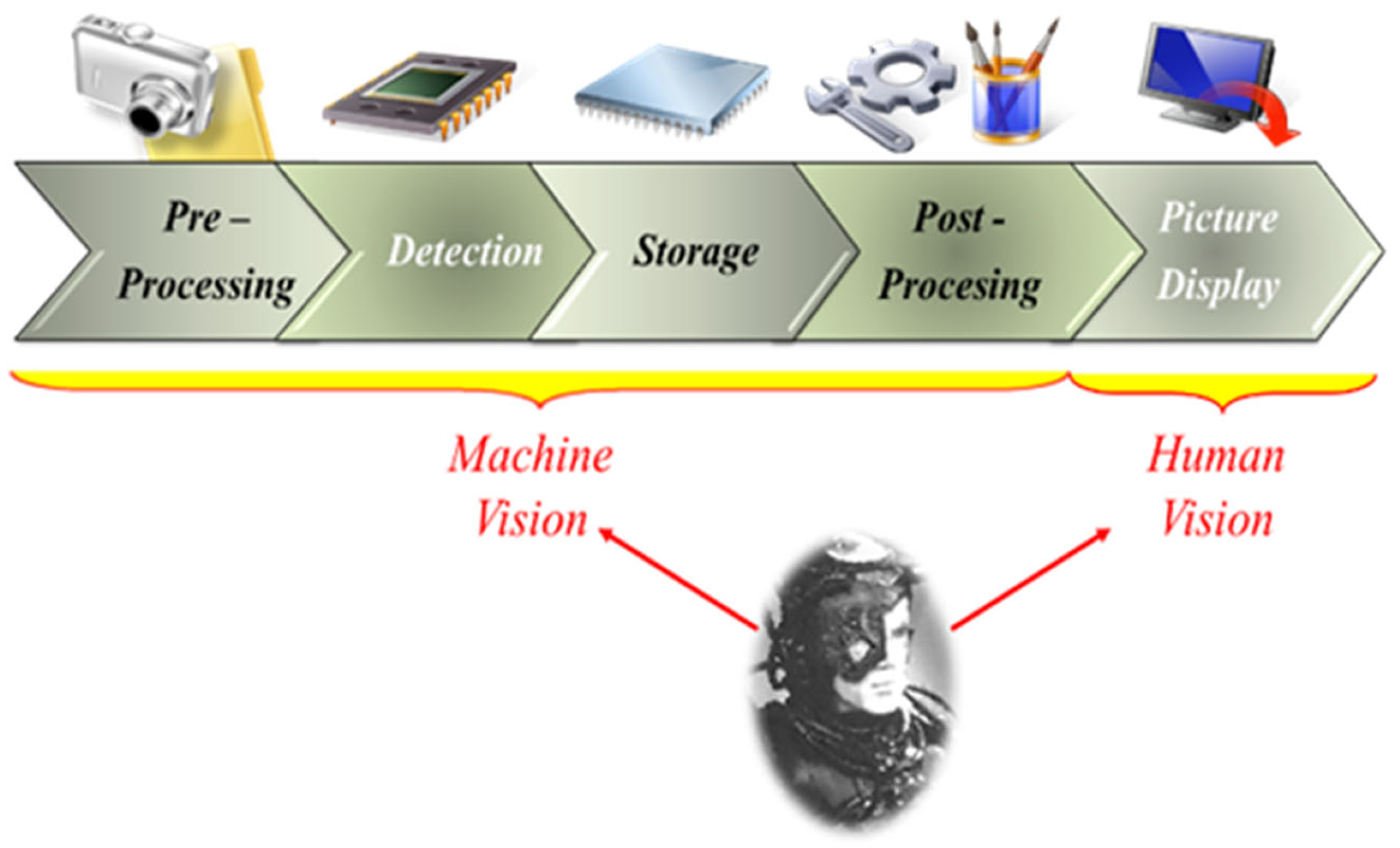
Figure 6.
Based on the mathematical analogy between the out-of-focus OTF and the ambiguity function, one can visualize the impact of focus error (on the OTF) in a polar display.
Figure 6.
Based on the mathematical analogy between the out-of-focus OTF and the ambiguity function, one can visualize the impact of focus error (on the OTF) in a polar display.
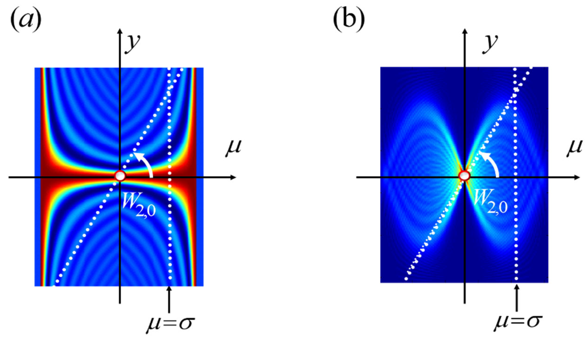
Figure 7.
Three dimensional graphs for visualizing the influence of focus error on the OTF. In (a), we consider a clear pupil aperture. In (b), the pupil aperture is covered with a mask that reduces the influence of focus errors. It is to be noted that the mask generates practically the same frequency response, if the focus error coefficient is in the interval (- 2 λ, 2 λ).
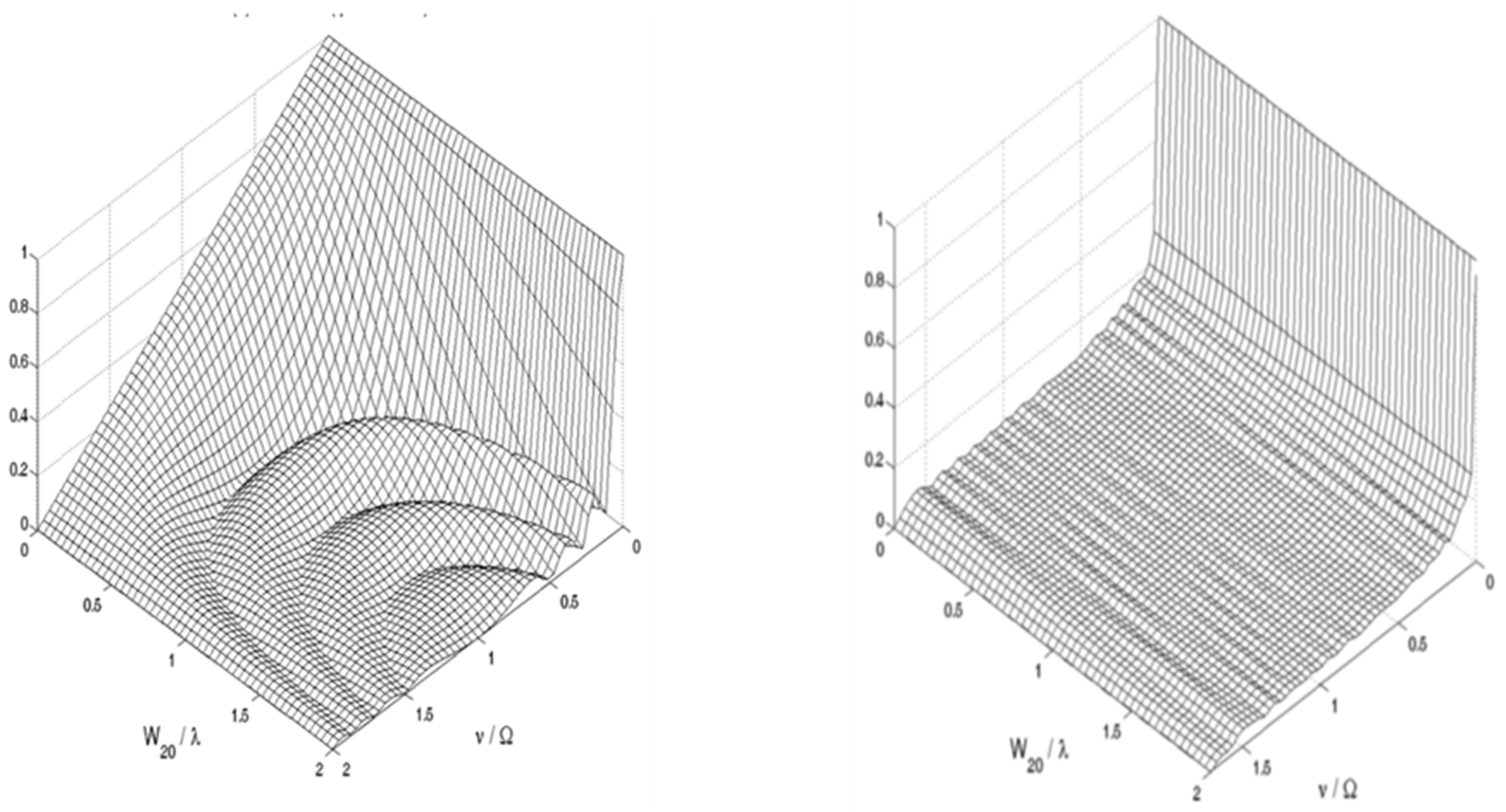
Figure 9.
Tunable amplification of the phase delays of a sinusoidal phase grating. In (a), the ratio of the amplification as a function of the lateral shift, β. In (b), the variations of the amplitudes, In blue the initial sinusoidal profile. In red, the final sinusoidal profile.
Figure 9.
Tunable amplification of the phase delays of a sinusoidal phase grating. In (a), the ratio of the amplification as a function of the lateral shift, β. In (b), the variations of the amplitudes, In blue the initial sinusoidal profile. In red, the final sinusoidal profile.
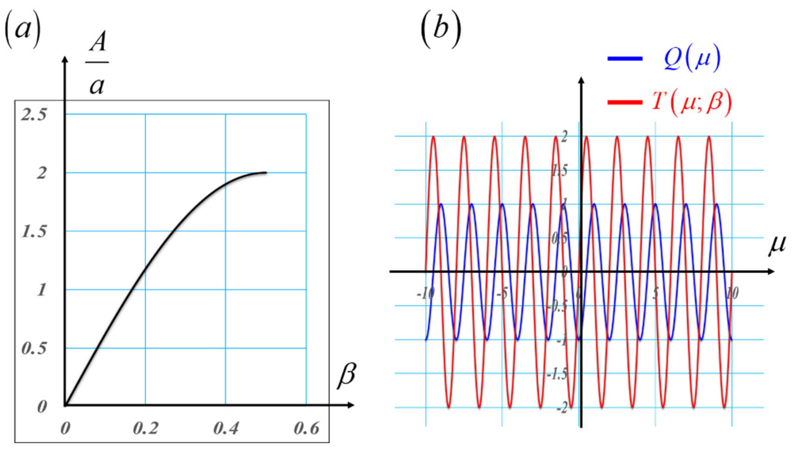
Figure 10.
Graphs depicting the variation of the optical path difference as one laterally shifts the phase conjugated masks. In (a), we show the lateral displacement between two phase conjugate masks. In (b), in blue, we depict the initial phase variation. And in red, we display the final phase variation. In (c), we exhibit a different value for the lateral shift. In (d), as in (b), we show the initial variation as well as the final variation.
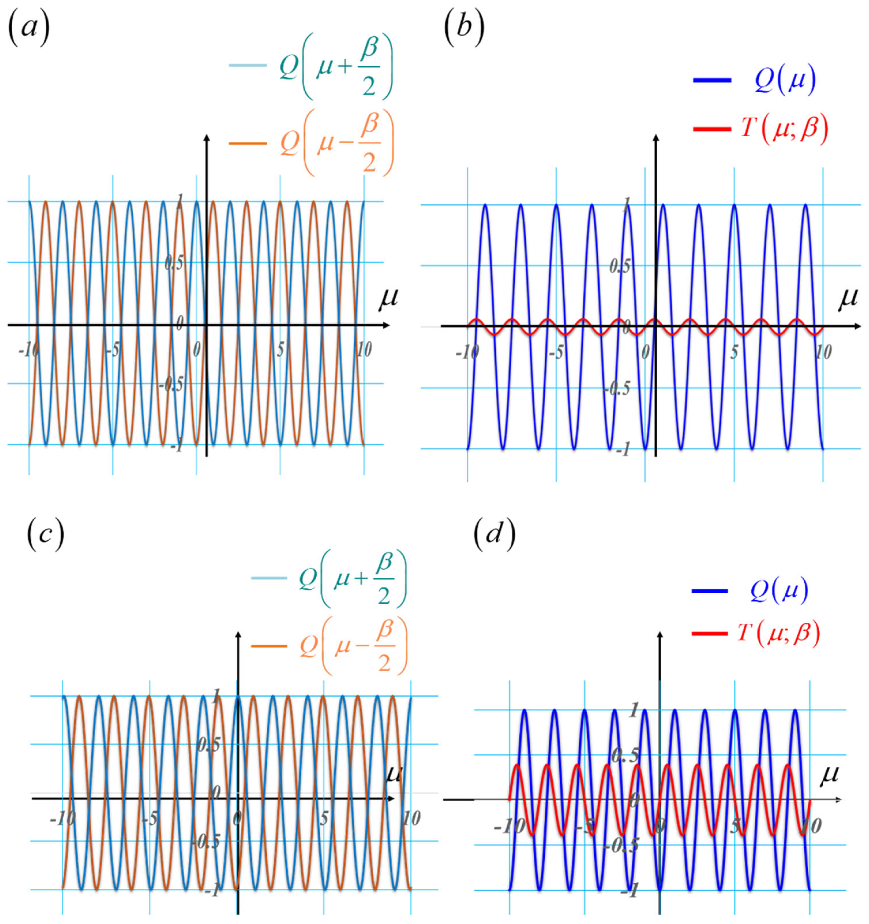
Figure 11.
Graphs showing the phase variations with hyperbolic profiles. In (a) in red a hyperbolic cosine variation, In blue a hyperbolic phase variation. In (b), the amplification ratio that can be achieved by using the hyperbolic phase profile in Equation (18).
Figure 11.
Graphs showing the phase variations with hyperbolic profiles. In (a) in red a hyperbolic cosine variation, In blue a hyperbolic phase variation. In (b), the amplification ratio that can be achieved by using the hyperbolic phase profile in Equation (18).
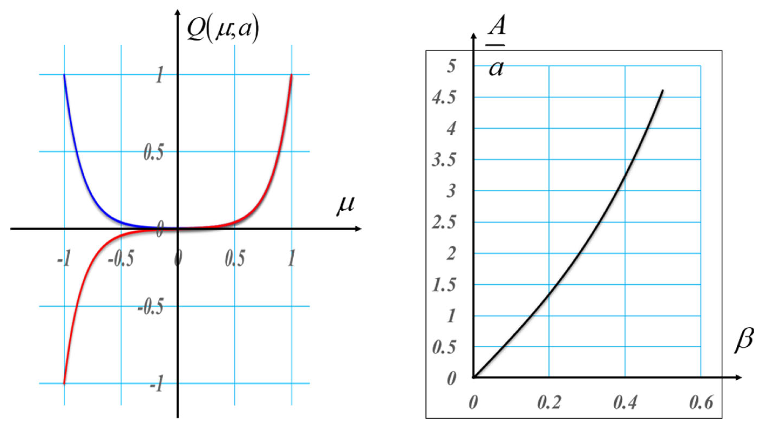
Figure 12.
Graphs showing the changes in optical path difference if two conjugate hyperbolic masks are laterally shifted, as in Equation (17). In blue the initial hyperbolic cosinusoidal mask. In red the generated hyperbolic sinusoidal mask.
Figure 12.
Graphs showing the changes in optical path difference if two conjugate hyperbolic masks are laterally shifted, as in Equation (17). In blue the initial hyperbolic cosinusoidal mask. In red the generated hyperbolic sinusoidal mask.
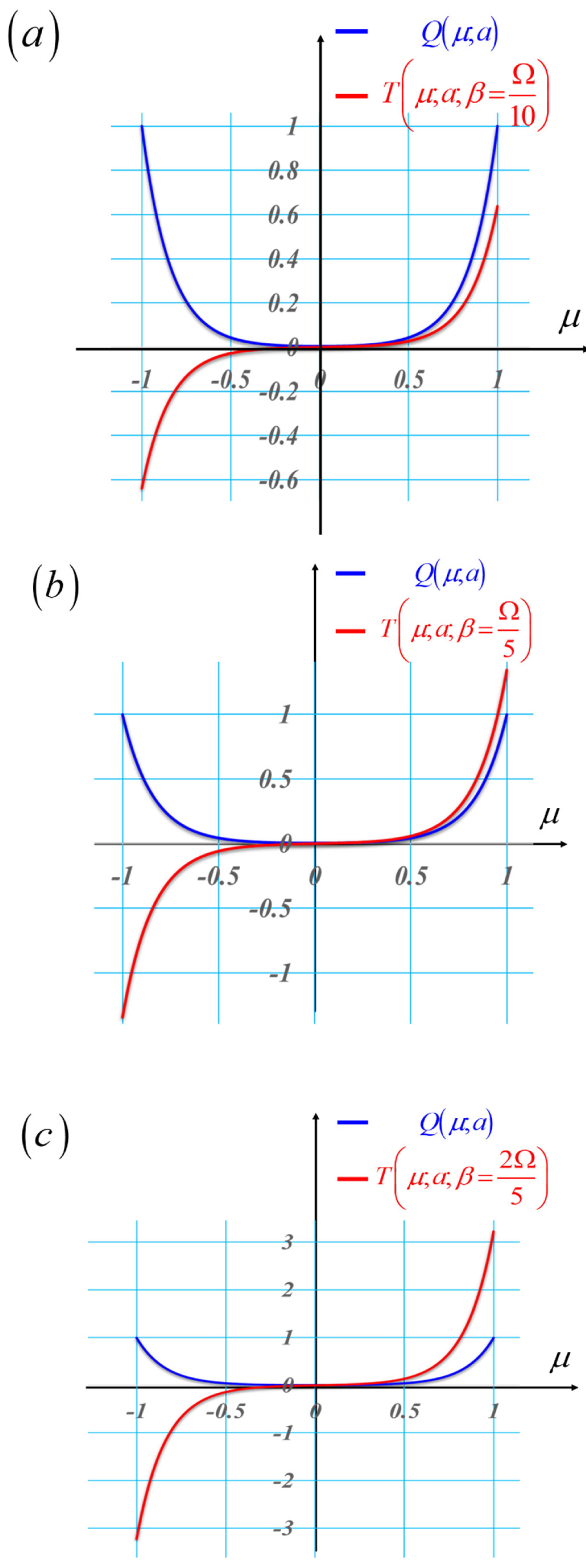
Figure 13.
Graphs displaying the impact on the MTF of the tunable hyperbolic mask in Equation (17). In (a), the MTFs of a clear pupil aperture with focus error coefficients with values equal to 0, λ, 2 λ, and 3 λ. In (b), the MTFs of a hyperbolic phase mask for the same values in (a) of the focus error coefficients. It is apparent from (b) that the MTFs vary slowly with the variations of focus errors.
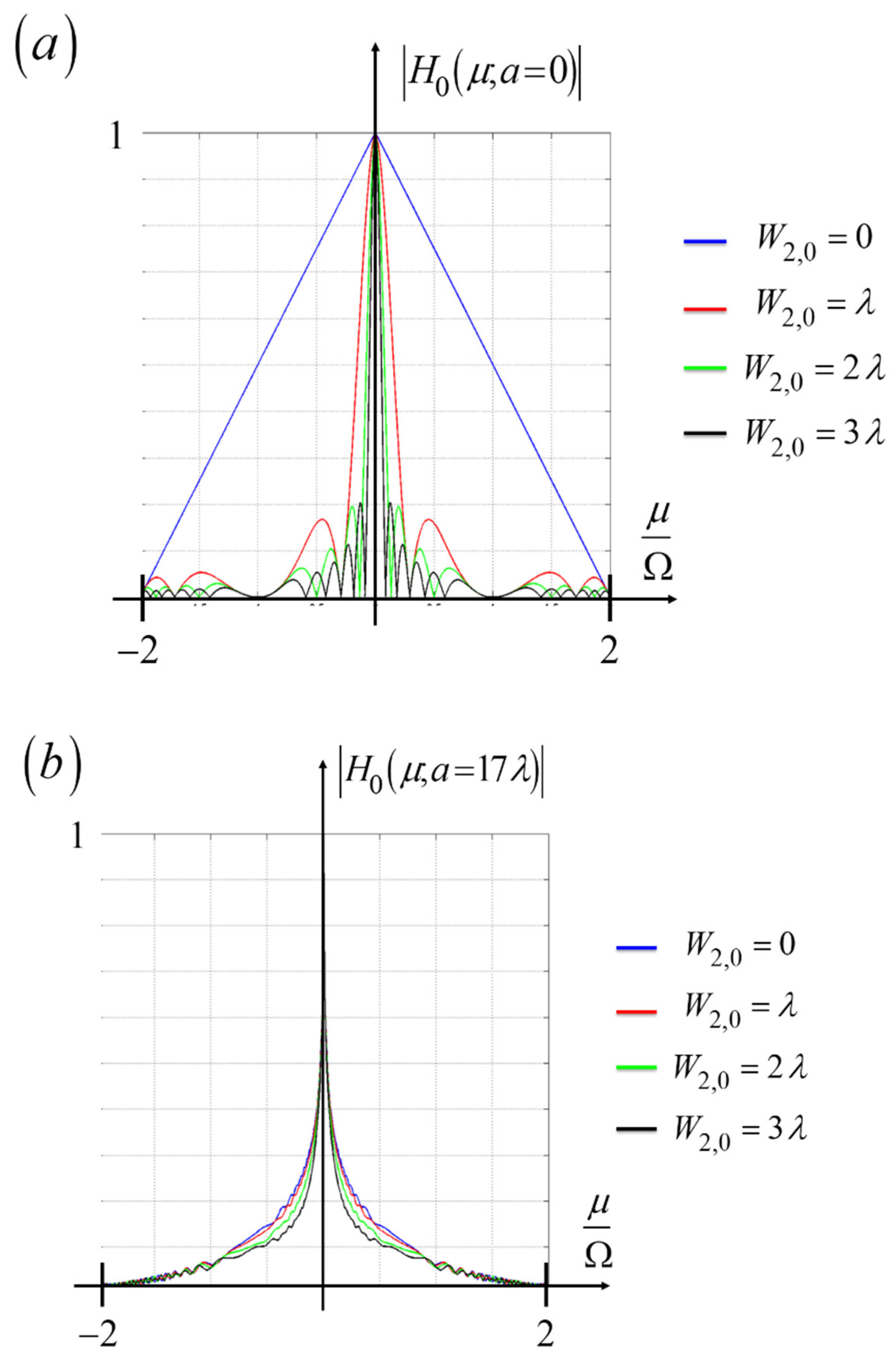
Figure 14.
Schematics like that in Figure 8. Now, we use a vortex pair for generating tunable optical path differences with prespecified radial profile R(ρ).
Figure 14.
Schematics like that in Figure 8. Now, we use a vortex pair for generating tunable optical path differences with prespecified radial profile R(ρ).
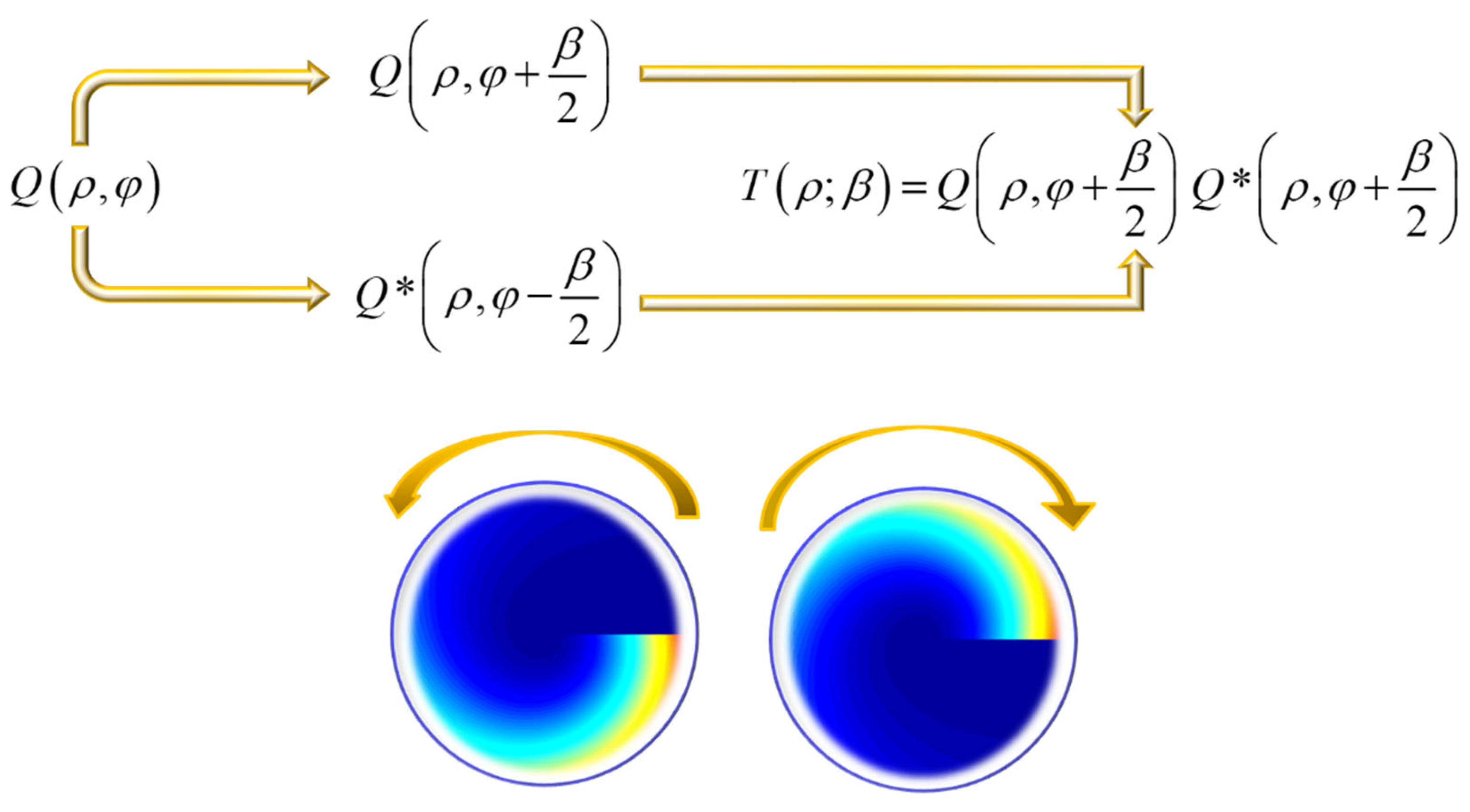
Figure 15.
Pictorial showing the use of a pair of masks for controlling th optical path difference. At the Fourier domain, we represent the masks by their interferograms. The pictorial incorporates the pair of interferograms in rectangular coordinates, as well as the pair in polar coordinates.
Figure 15.
Pictorial showing the use of a pair of masks for controlling th optical path difference. At the Fourier domain, we represent the masks by their interferograms. The pictorial incorporates the pair of interferograms in rectangular coordinates, as well as the pair in polar coordinates.
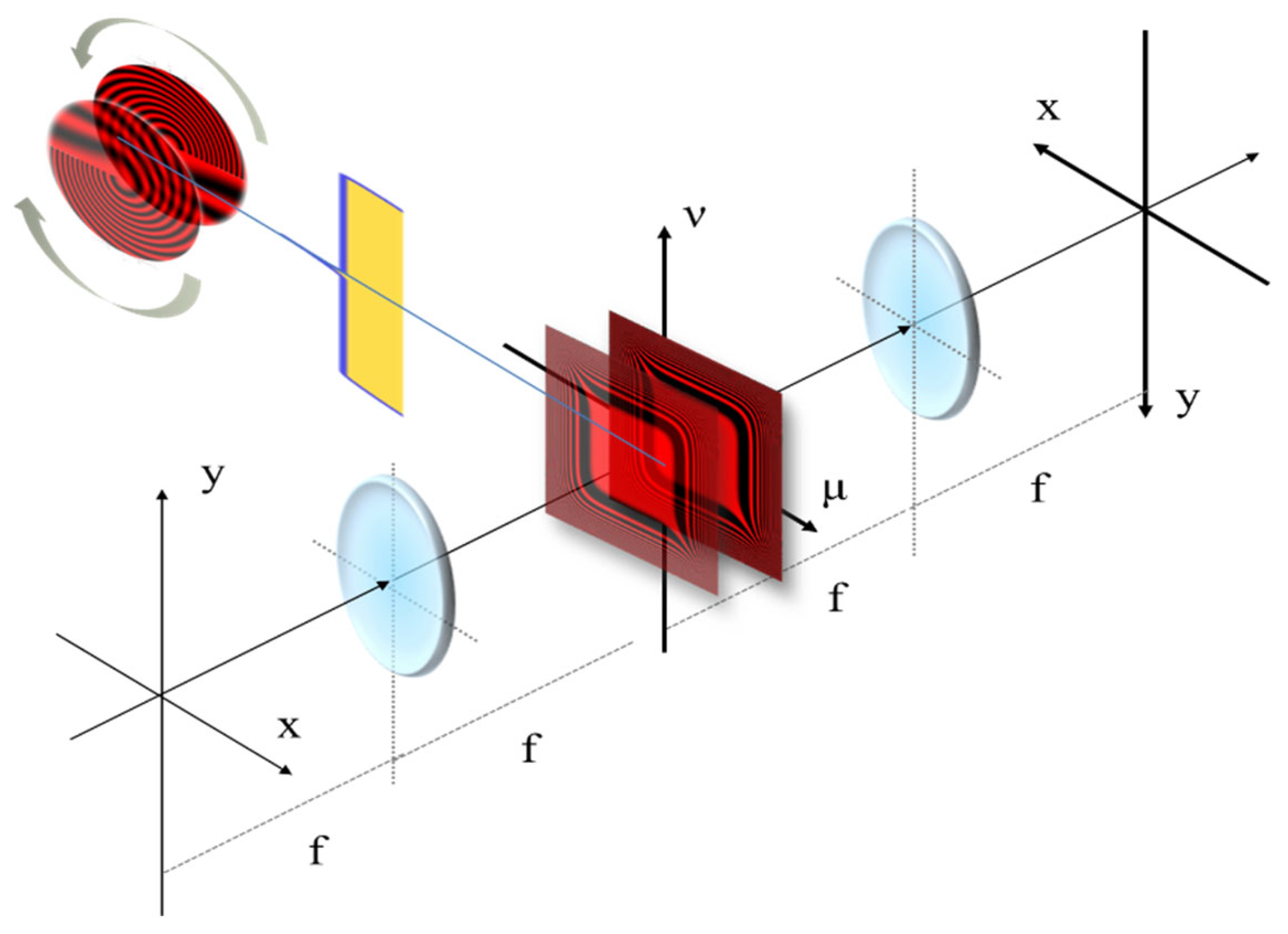
Figure 17.
Schematics on the use of a pair of masks coded with the Barker sequences. For narrowing the width of the windows on the OTF, the coded masks substitute a pair of slits. In(a), a pair of slits. In (b), the OTF windows obtained by using the slits. In (c), we substitute the slits by masks coded with the Barker sequences. In (d), the OTF windows obtained by using the masks coded with the Barker sequences.
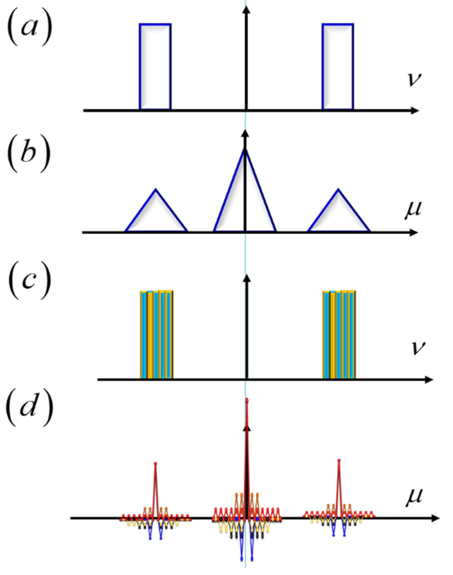
Figure 18.
Pictorial of an optical system for gathering images in Moiré photography. The optical masks implement transparent windows on the OTF. At the upper part, the slits mask proposedby Burch. In the lower part, the masks coded with theBarker sequences.
Figure 18.
Pictorial of an optical system for gathering images in Moiré photography. The optical masks implement transparent windows on the OTF. At the upper part, the slits mask proposedby Burch. In the lower part, the masks coded with theBarker sequences.
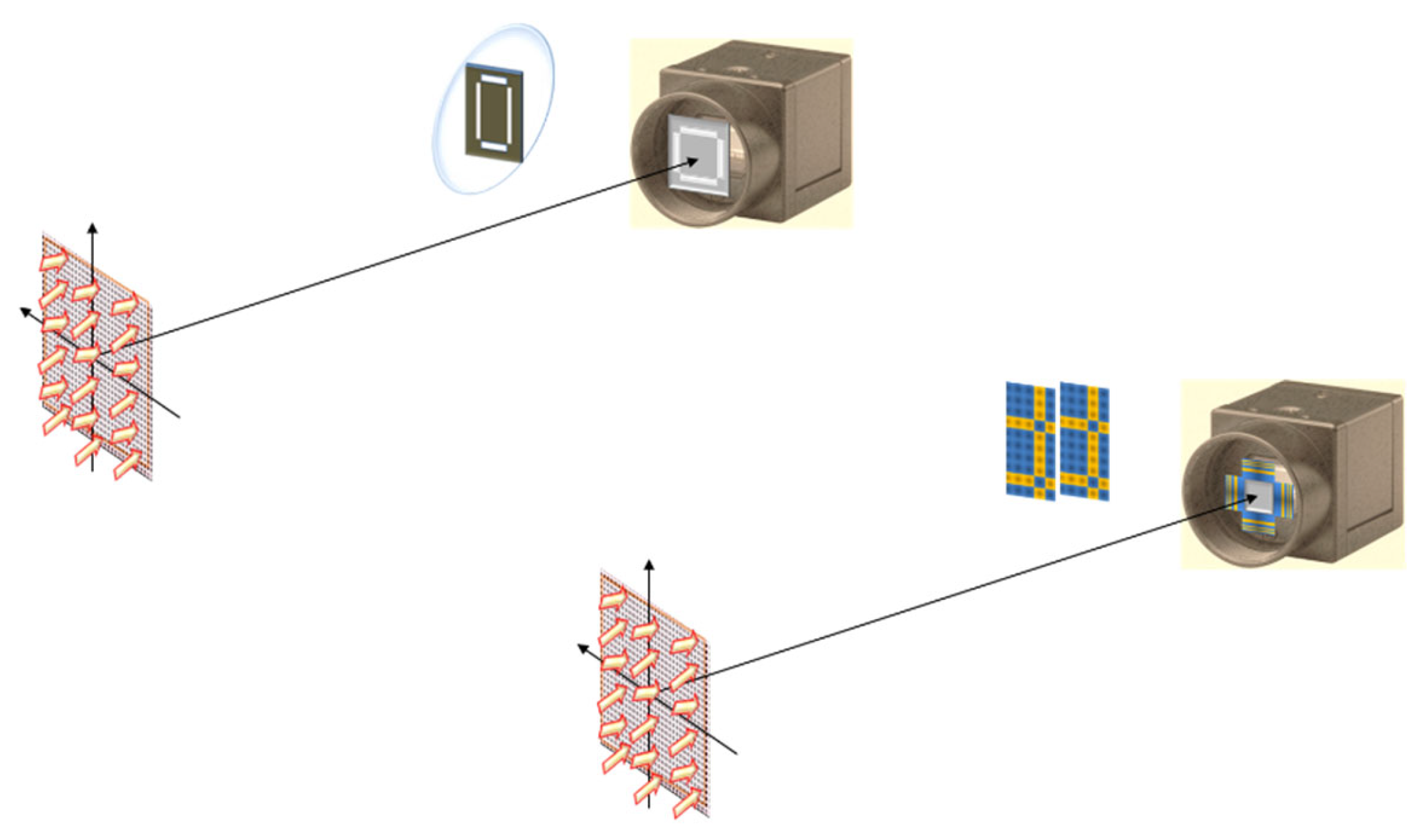
Figure 19.
Display of the 2-D optical masks that are coded with the Barker matrices.
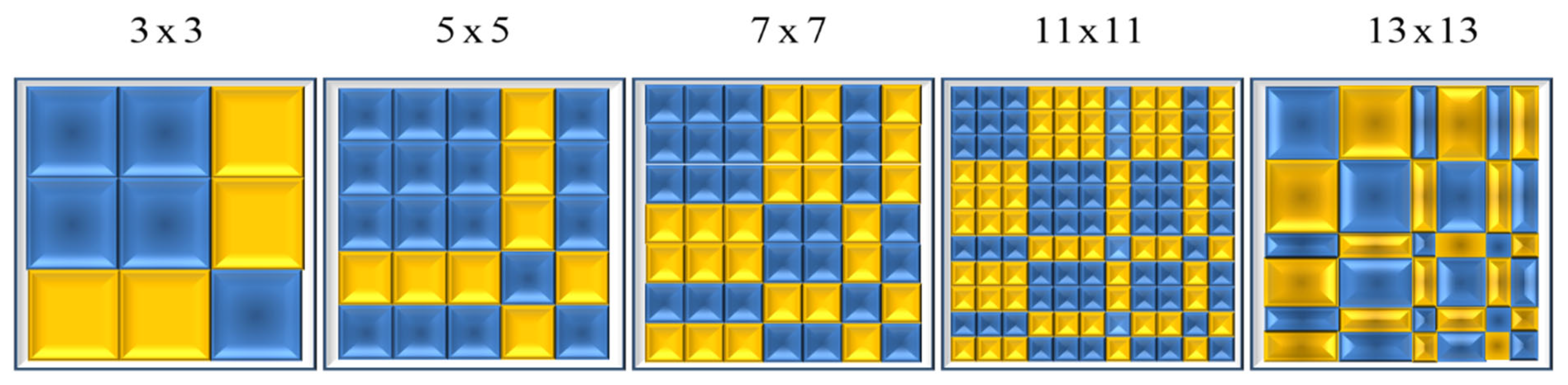
Figure 20.
Optical masks coded angularly with the Barker sequences.
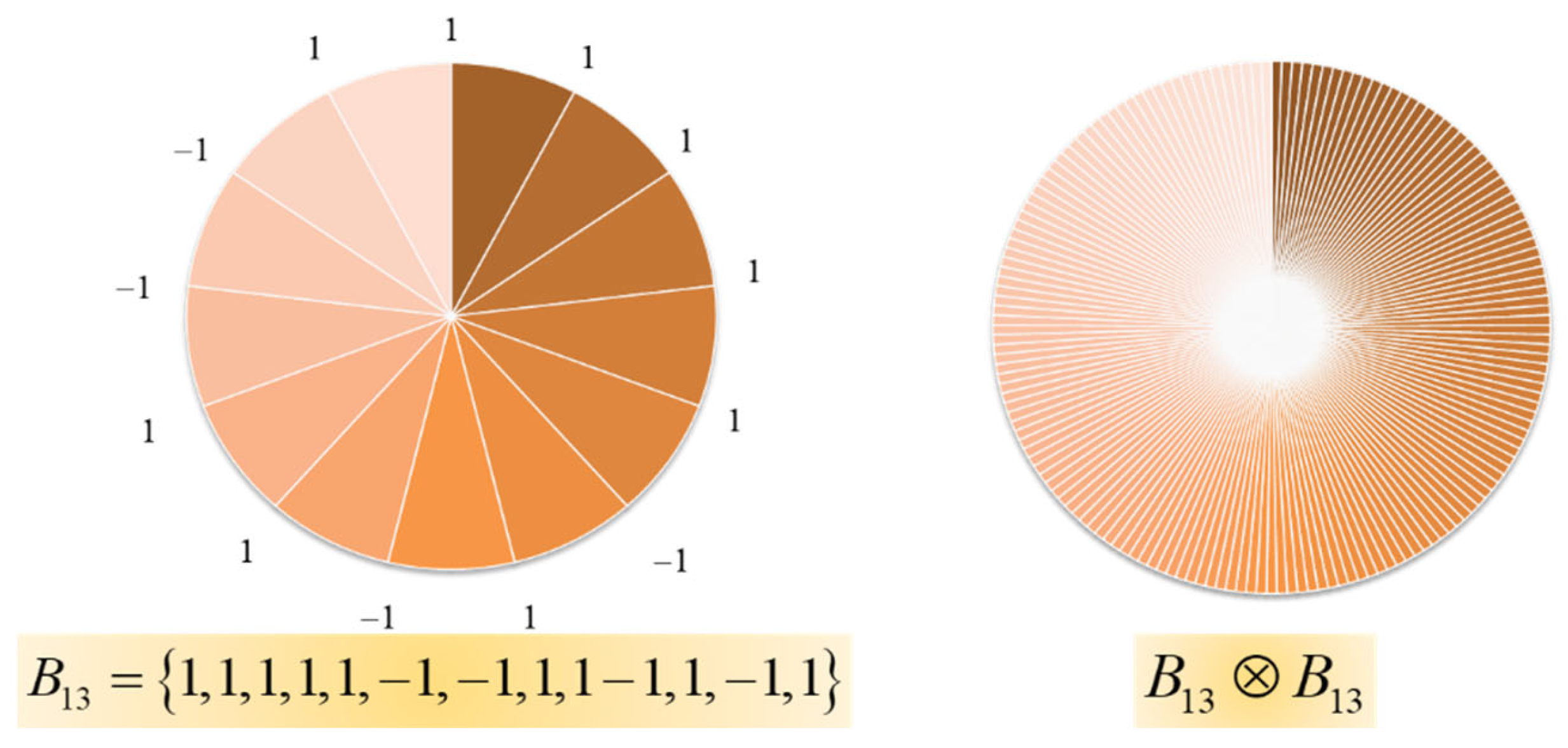
Figure 21.
Optical zone plates that are coded radially and angularly with the Barker sequences.
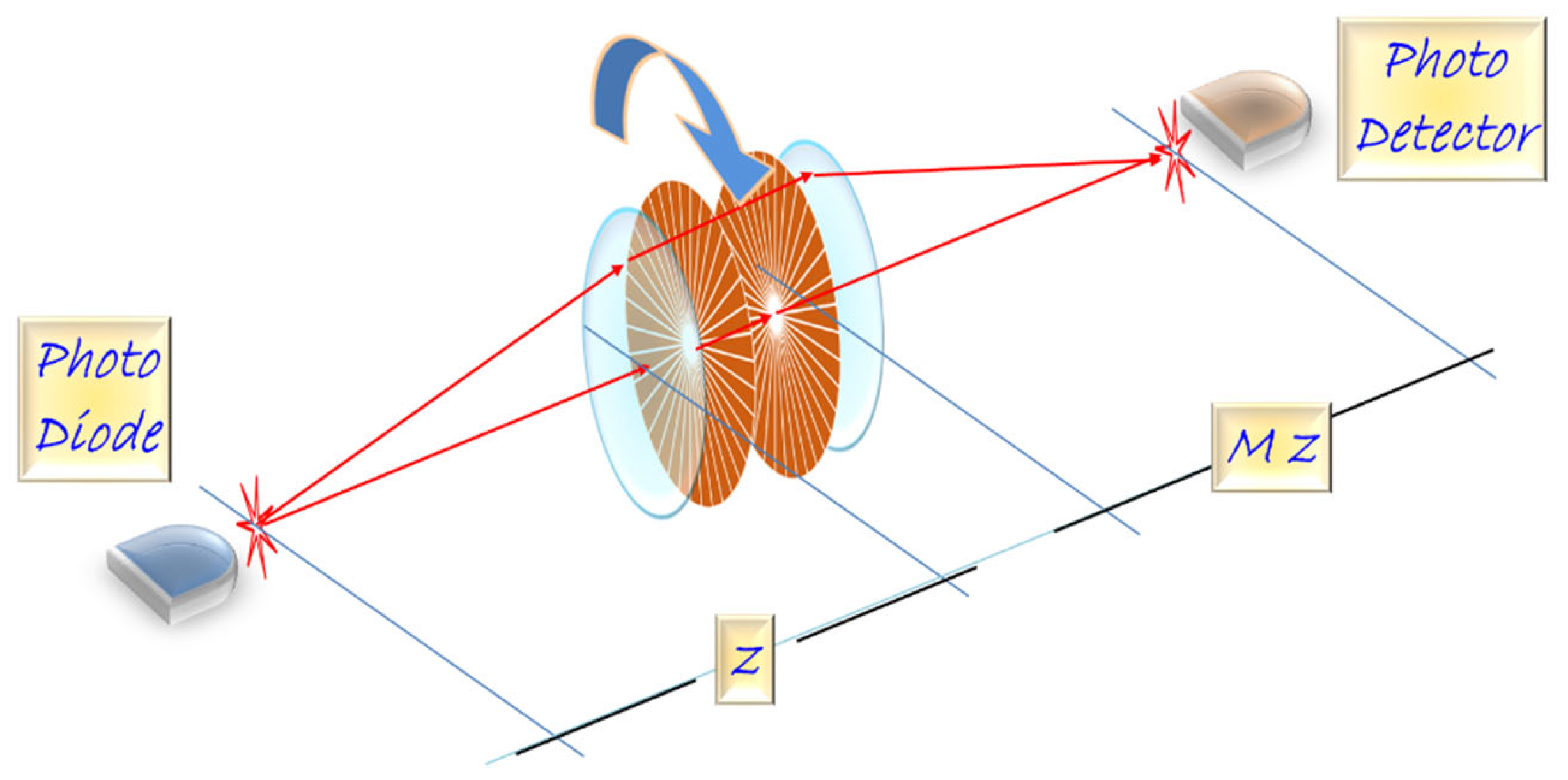
Figure 22.
Optical zone plates that are coded radially and angularly with the Barker sequences.
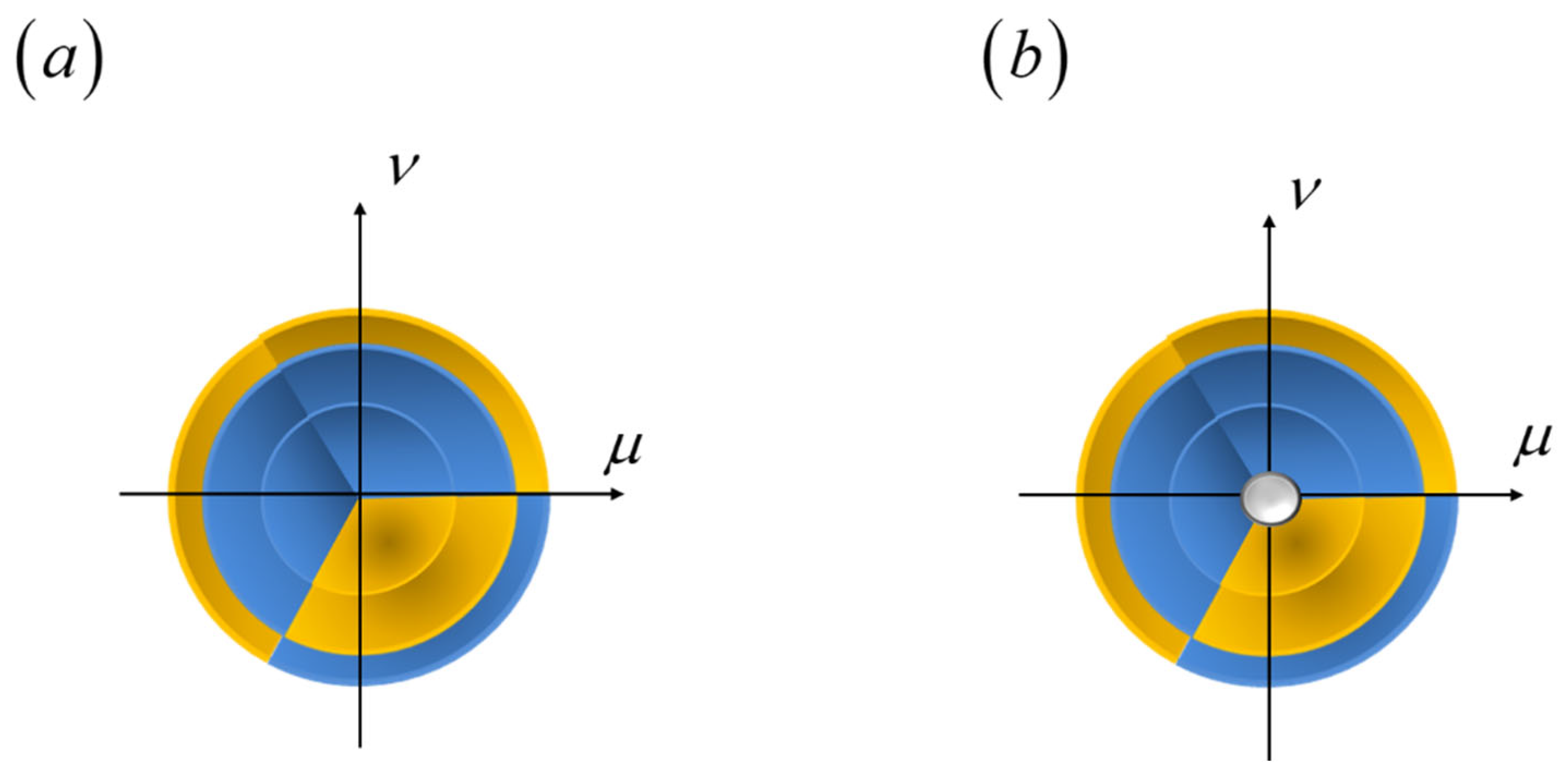
Figure 23.
Schematics of the optical setup depicting the use of a single varifocal lens for tuning the magnification with fixed throw T. In (a), as the optical power changes, one needs to move the lens longitudinally. In (b) we display the use of two varifocal lenses for generation tunable magnifications at the input plane. That is, the two varifocals implement a zero-throw tunable mangnification. In (c), we show the use of two varifocal lenses for tuning the magniticiton at back focal plane of the initial lens. This lens has a fixed optical power. The pair of varifocals generate a zero-throw, tunable Barlow lens.
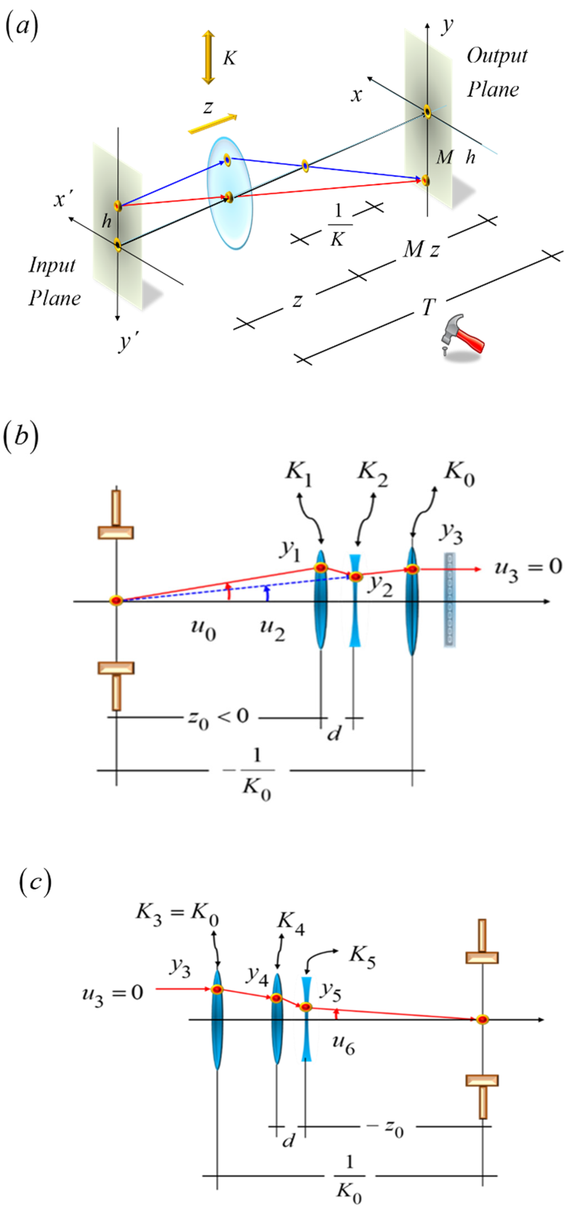
Figure 26.
Computer simulations of the tunable anamorphic magnifications. In (a), the absolute value of the magnification in x is the same than absolute value of the magnification in y. That is, | Mx |=| My |. In (b), | Mx | >| My |. In (c), | Mx | < | My |.
Figure 26.
Computer simulations of the tunable anamorphic magnifications. In (a), the absolute value of the magnification in x is the same than absolute value of the magnification in y. That is, | Mx |=| My |. In (b), | Mx | >| My |. In (c), | Mx | < | My |.
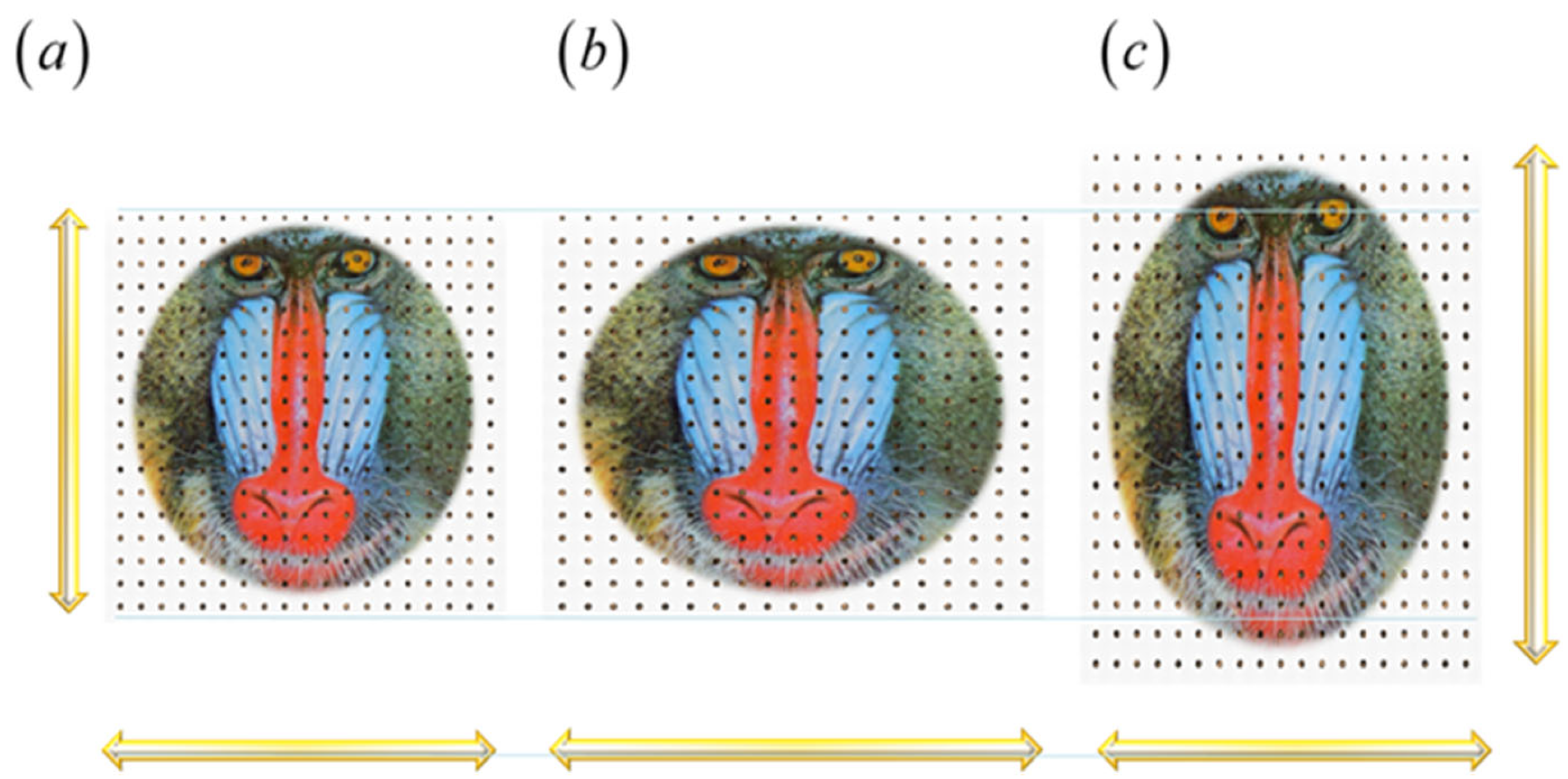

Table 1.
We list some of the Barker sequences that are employed in our current discussion.
 |
Disclaimer/Publisher’s Note: The statements, opinions and data contained in all publications are solely those of the individual author(s) and contributor(s) and not of MDPI and/or the editor(s). MDPI and/or the editor(s) disclaim responsibility for any injury to people or property resulting from any ideas, methods, instructions or products referred to in the content. |
© 2025 by the authors. Licensee MDPI, Basel, Switzerland. This article is an open access article distributed under the terms and conditions of the Creative Commons Attribution (CC BY) license (http://creativecommons.org/licenses/by/4.0/).
Copyright: This open access article is published under a Creative Commons CC BY 4.0 license, which permit the free download, distribution, and reuse, provided that the author and preprint are cited in any reuse.


