
Submitted:
24 August 2025
Posted:
25 August 2025
You are already at the latest version
Abstract
To address the challenge of efficiently identifying and providing early warnings for typical structural damages in small and medium-sized bridges during long-term service, this paper proposes an intelligent monitoring and recognition method based on ultra-weak fiber Bragg grating (UWFBG) array sensing. By deploying UWFBG strain-sensing cables across the bridge, the system enables continuous acquisition and spatial analysis of multi-point strain data. Based on this, a series of experimental scenarios simulating typical structural damages—such as single-slab loading, eccentric loading, and bearing detachment—are designed to systematically analyze strain evolution patterns before and after damage occurrence. While strain distribution maps allow for visual identification of some typical damages, the approach remains limited by reliance on manual interpretation, low recognition efficiency, and weak detection capability for atypical damages. To overcome these limitations, machine learning algorithms are further introduced to extract features from strain data and perform pattern recognition, enabling the construction of an automated damage identification model. This approach enhances both the accuracy and robustness of damage recognition, achieving rapid classification and intelligent diagnosis of structural conditions. The results demonstrate that the integration of the monitoring system with intelligent recognition algorithms effectively distinguishes different types of damage and shows promising potential for engineering applications.
Keywords:
ultra-weak FBG array sensing
; small and medium-sized bridges
; typical defects monitoring
; intelligent identification
1. Introduction
As a critical component of China’s highway bridge infrastructure, small and medium-sized bridges play a central role in the national transportation network. According to the 2024 Statistical Bulletin on the Development of the Transportation Industry, by the end of 2024, the total number of highway bridges nationwide had reached 1.1081 million, with a total length of 101.9758 million meters. Among them, extra-large and large bridges account for less than 20%, with the vast majority being small and medium-sized bridges. These structures are widely distributed across urban-rural fringes, mountainous regions, and ordinary arterial roads. Due to complex service environments and limited maintenance resources, they are often subjected to high-frequency loading and environmental degradation, making them prone to typical structural damages such as bearing anomalies, eccentric loading, and single-slab stress conditions [1]. These defects not only reduce local structural stiffness and degrade load-bearing capacity but also pose significant risks to traffic safety. For instance, in 2019, a severe eccentric load caused the overturning of an elevated bridge in Wuxi, Jiangsu Province, resulting in multiple vehicles being crushed and casualties, which attracted widespread public concern.
In light of the vast number, wide distribution, and high detection difficulty of such bridges, achieving rapid sensing, accurate identification, and intelligent early warning of structural conditions has become a critical challenge in the field of bridge health monitoring [2]. Traditional inspection methods mainly rely on manual experience and a limited number of measurement points. These approaches suffer from discontinuous deployment, strong subjectivity in diagnosis, and poor real-time performance, making them inadequate for the comprehensive, accurate, and timely monitoring required by small and medium-sized bridge applications [3,4].
In recent years, optical fiber sensing technology has achieved significant advancements in the field of civil engineering monitoring. Among these, the Fiber Bragg Grating (FBG) sensor has emerged as a key tool for structural health monitoring due to its advantages, including high sensitivity, immunity to electromagnetic interference, corrosion resistance, and long-distance signal transmission [5,6,7]. Currently, the predominant distributed optical fiber sensing techniques are primarily based on Brillouin scattering and Rayleigh scattering effects. Although these methods support continuous spatial deployment, they still exhibit limitations in terms of sensing sensitivity, bandwidth, and system complexity [8]. In contrast, FBG array sensing based on ultra-weak reflectivity utilizes micro-reflective units with reflectivity as low as one-thousandth of standard gratings. This design ensures uninterrupted signal transmission and allows for the multiplexing of hundreds or even thousands of sensing nodes along a single fiber [9]. Such high-density deployment enables superior performance in synchronous multi-point strain sensing and distributed response identification, making it particularly well-suited for engineering applications involving complex structural forms and constrained monitoring spaces—such as small and medium-sized bridges.
By constructing FBG arrays, high spatial-resolution, multi-point continuous strain monitoring can be achieved along the entire length of a bridge. This approach offers advantages such as flexible deployment, a large number of sensing nodes, and strong data stability, providing reliable support for the localization of typical structural damages and the analysis of their progression trends [10,11]. However, two key challenges remain in practical monitoring applications: (1) the diversity of damage types and the complexity of associated strain distribution patterns make manual interpretation of strain maps highly subjective and inefficient; (2) atypical or weakly distributed damages are difficult to identify through visual inspection, increasing the risk of missed or incorrect diagnoses.
To address these issues, machine learning algorithms have been increasingly adopted in the field of structural health monitoring for bridges. By enabling automated feature extraction and classification modeling of spatiotemporal strain data, these algorithms demonstrate strong potential in recognizing complex data patterns, significantly improving the accuracy and real-time performance of structural anomaly detection [12,13]. Current research primarily focuses on two major areas. The first involves damage detection based on image recognition, which employs computer vision and image processing techniques to identify visible defects such as cracks, spalling, and corrosion [14,15,16,17,18]. The second pertains to internal defect monitoring through sensor signal analysis, utilizing technologies such as ultrasonic testing [19], infrared thermal imaging [20], electromagnetic induction [21], and fiber optic sensing [22] to detect concealed structural issues, including internal cracks, voids, and steel reinforcement corrosion. Furthermore, in recent years, artificial intelligence has gained increasing prominence in civil engineering applications. Deep learning models such as Convolutional Neural Networks (CNNs) and You Only Look Once (YOLO) have been applied to crack detection and defect classification, resulting in notable improvements in both recognition accuracy and processing speed [23,24,25,26].
Based on these insights, this paper proposes a damage monitoring and intelligent identification method for small and medium-sized bridges that integrates UWFBG array sensing with machine learning techniques. By deploying UWFBG array strain-sensing cables along the full length of the bridge, the system enables continuous acquisition and spatial analysis of multi-point strain data. In the data processing stage, a damage identification model is developed using the Random Forest (RF) algorithm as the core classifier, while Extreme Gradient Boosting (XGBoost) and Support Vector Machine (SVM) models are introduced as comparative methods to comprehensively evaluate classification performance and robustness. The experimental design includes simulations of typical damage scenarios such as single-slab loading, various eccentric loading conditions, and bearing detachment. Key feature parameters are extracted to construct the classification framework, enabling automatic identification and categorization of damage states. The results demonstrate that the proposed method not only achieves high accuracy and stability in damage recognition but also features a lightweight system structure and easy deployment. It is particularly well-suited for routine monitoring and disaster early warning of small and medium-sized bridges, showing strong potential for practical engineering applications.
2. Principles of FBG Array Sensing and Machine Learning
2.1. Principle of FBG Array Sensing
FBG is a passive optical device formed by permanently inducing a periodic modulation of the refractive index in the core of an optical fiber through specific fabrication methods, such as two-beam interference, amplitude masking, or point-by-point inscription. Essentially, it is a section of optical fiber in which the refractive index of the core is periodically altered, while the cladding remains unchanged. When a broadband light signal propagating along the fiber encounters the grating, diffraction occurs: the portion of the incident light whose wavelength matches the Bragg wavelength of the grating is reflected, whereas light at other wavelengths continues to transmit unaffected [27].
According to coupled-mode theory, the Bragg wavelength of an FBG can be expressed as [28]:
where represents the center wavelength of the FBG; represents the effective refractive
index of the fiber core; represents the grating period.
Both and are affected by temperature and strain. Therefore, when the external environment induces changes in temperature or mechanical stress within the grating region, the Bragg wavelength shifts accordingly.
In this study, a distributed UWFBG array sensing cable is employed as the core sensing unit. The armored cable contains a continuous array of UWFBG strain sensors, composed of n weak gratings with no fusion splices, each corresponding to a 1-meter-long sensing segment. Using time-division multiplexing (TDM) demodulation technology, the system measures structural strain by detecting the wavelength shift of reflected signals from the weak gratings. Simultaneously, the time-of-flight of the reflected signal is used to locate the exact position of each sensing segment, as illustrated in Figure 1.
2.2. Principles of Machine Learning
With the significant increase in the dimensionality and complexity of structural monitoring data, traditional rule-based matching and threshold-based judgment methods have become insufficient for meeting the demands of state recognition under complex working conditions. Machine learning algorithms, by contrast, offer efficient classification and intelligent recognition of structural health status through mechanisms such as automated feature extraction, nonlinear mapping, and adaptive learning. In this study, three representative supervised learning algorithms—RF,XGBoost,and SVM—are selected as the foundation for constructing damage identification models. The specific principles are as follows.
2.2.1. Random Forest
RF is an ensemble learning method created by Tin Kam Ho [29] in 1995, which serves as a typical representative under the Bagging framework. The core concept involves improving the accuracy and robustness of the overall model by constructing multiple decision trees and combining their output through voting or averaging mechanisms, as illustrated in Figure 2. Compared to a single decision tree, which is prone to overfitting and poor generalization, RF effectively reduces variance through ensemble modeling and exhibits strong robustness to noise.
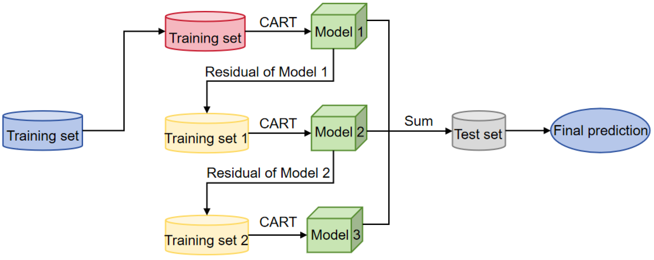
2.2.2. XGBoost
XGBoost is an ensemble learning algorithm based on the Gradient Boosting framework, proposed by Tianqi Chen et al. in 2014 [30]. As an efficient implementation of Gradient Boosted Decision Trees (GBDT), XGBoost employs an additive model and a forward stage-wise optimization strategy. It iteratively constructs multiple weak learners and combines them into a strong learner, thereby enhancing predictive accuracy while maintaining fast training speed. Compared to traditional GBDT, XGBoost introduces a regularization term into the model structure, which effectively controls model complexity and mitigates the risk of overfitting.
Figure 3.
Workflow of the XGBoost Algorithm.
2.2.3. Support Vector Machine
SVM is a classical supervised learning method initially proposed by Vladimir Vapnik et al. in 1964 [31]. It belongs to the category of maximum margin classifiers. The core idea of SVM is to construct an optimal hyperplane in a high-dimensional feature space, such that this hyperplane not only accurately separates data samples of different classes but also maximizes the margin between classes, thereby enhancing the model’s generalization ability, as illustrated in Figure 4.This method is particularly well-suited for scenarios with high-dimensional feature spaces and relatively small sample sizes.
3. Damage Simulation Experiment and Feature Extraction
3.1. Damage Simulation Experiment
3.1.1. Optical Fiber Cable Layout Scheme
Considering that the test bridge is a single-lane scaled-down model, the monitoring layout follows the principle of "inner and outer circles surrounding and upper and lower surfaces synchronized." Specifically, an optical cable is laid on both the inner and outer sides of the bridge, while sensor cables are installed on both the bridge deck and the bridge underside to achieve synchronized strain data collection from both surfaces. Given that the total length of the bridge is 137.3 meters, a single optical cable can cover both the inner and outer loops, fulfilling the dual requirements of spatial continuity and cost efficiency.
Based on the structural characteristics of different bridge types, the experiment adopted optimized cable deployment strategies: For the simply supported bridge, a folded-back layout was used on the underside, with cables embedded beneath the three slabs to facilitate the identification of localized strain anomalies caused by single-slab loading. For the steel girder bridge, due to its metallic surface and the need to avoid damaging the structure, cables were surface-mounted, ensuring structural integrity. For the simply supported bridge surface, cables were embedded in pre-cut grooves, allowing them to deform synchronously with the bridge and improving the fidelity of strain response. The specific deployment strategies and cable routing schemes are shown in Figure 5 and Figure 6.
3.1.2. Experimental Conditions
The experiments were conducted on both simply supported bridge and steel girder bridge models to simulate various common structural defects, including single-slab loading, bearing detachment, and eccentric loading. In each test, a forklift was used as the loading vehicle, with additional counterweights (each weighing 200 kg) applied to simulate diverse load scenarios. The forklift traversed the bridge deck under three loading conditions: without counterweights, with one counterweight, and with two counterweights.
The specific loading conditions are summarized in Table 1, covering different types of structural defects and their coupling effects with varying load levels.
3.1.3. Damage Simulation Methods
- Single-slab Loading Simulation: To replicate localized load concentration issues common in simply supported slab bridges, the test bridge deck was composed of three slabs of equal dimensions. The inner slab was physically separated from the adjacent slabs by creating a visible structural gap, enabling it to bear the load independently during loading. This setup simulates a typical “single-slab loading concentration” scenario.
- Eccentric Loading Simulation: Eccentric loading conditions were simulated on the steel girder bridge by operating the loading vehicle along paths offset from the centerline of the deck. Two types of eccentricity were considered: inner and outer eccentric loads, which represent uneven structural responses caused by off-centered vehicle loading.
- Bearing Detachment Simulation: Bearing detachment or failure is a common yet hard-to-detect hazard during bridge operation, potentially causing localized deck settlement or global redistribution of structural forces. A jack and shims were placed beneath the outer bearing of Pier No. 7 on the steel girder bridge. By gradually lifting the bearing and removing the shims, the bearing transitioned from a load-bearing to a partially detached state, inducing a suspended condition at the support and leading to abnormal stress concentrations.
The on-site layout of each damage simulation setup is illustrated in Figure 7.
3.2. Feature Extraction and Label Assignment
To facilitate machine learning modeling for defect identification, the original strain time series collected from optical fiber cables must be converted into feature vectors suitable for classification. Feature extraction is categorized based on bridge types and defect types, and includes the following four groups: features for single-slab loading, features for eccentric loading, features for bearing detachment, and features for weight configuration.
3.2.1. Feature Selection for Single-Slab Loading Identification
During vehicle passage over the simply supported bridge, the vehicle’s position significantly affects the strain distribution among the three underside optical fiber cables.
In this study, four statistical indicators—maximum, mean, standard deviation, and range—are extracted from the sensor data of underside cable to characterize the overall strain distribution. These four types of features can be expressed as:
In the equation, represents the sensor number,represents the start time, and represents the end time.
3.2.2. Feature Extraction for Eccentric Loading Identification
Under eccentric loading conditions, the force distribution across the two sides of the bridge structure becomes uneven, leading to discrepancies in the strain responses recorded by the sensors located on the inner and outer sides of the bridge underside. To capture these discrepancies, the following features are extracted: the differences in maximum values, mean values, standard deviations, and energy between the inner and outer sides, along with the respective maximum strain values. These features collectively characterize the asymmetry of lateral loading and assist in identifying the direction of eccentricity. The features are defined as follows:
In the equations, denotes the strain on the outer side, denotes the strain on the inner side, denotes the number of sensors on the outer side, and denotes the number of sensors on the inner side.
3.2.3. Feature Extraction for Bearing Detachment Identification
In the simulated bearing detachment experiments on the steel girder bridge, significant localized strain disturbances were observed near the underside support region. Therefore, the strain data from sensor No. 135, located near the bearing, is selected for analysis. Eight features are extracted—maximum, minimum, mean, standard deviation, range, energy, peak count, and slope variation—to capture the characteristics of local disturbances. These features are defined as follows:
Among these, .
3.2.4. Feature Extraction for Weight Level Identification
The addition of counterweights increases the overall stress level of the structure, resulting in enhanced strain responses. For the simply supported bridge, four statistical indicators from the underside strain data are extracted (Equations 2–5). For the steel girder bridge, the minimum deck strain and maximum underside strain are selected to distinguish the strain response under different weight levels. The selected features for the steel girder bridge are defined as:
where, and denote the minimum strain values measured by the sensor on the outer and inner sides of the bridge deck, respectively; and denote the maximum strain values measured by the sensor on the outer and inner sides of the bridge underside, respectively.
4. Model Construction and Evaluation
To achieve automatic identification and classification of typical bridge defects, this study constructs three types of classification models—RF, XGBoost, and SVM—based on the grating array strain data obtained from previous experiments. These models are developed and evaluated for four structural condition recognition tasks: single-slab loading identification, eccentric loading identification, bearing detachment identification, and weight level identification.
Specifically, the simply supported bridge is used to simulate single-slab loading and weight variation scenarios, while the steel girder bridge is employed to simulate bearing detachment and eccentric loading, with additional weight conditions introduced to enrich the classification labels. In each task, the model input consists of statistical features extracted from strain responses, and the output corresponds to the condition category label.
4.1. Modeling Process
Due to differences in data sources, structural characteristics, and loading schemes, the two bridges are modeled independently. Instead of uniformly constructing multi-label models, a task-splitting strategy was adopted, and binary or triple classification models were constructed for different defects respectively.
The overall modeling process includes data reading, feature extraction, label assignment, model training, performance evaluation, and result interpretation. As shown in Figure 8, the research framework is divided into separate modeling paths according to bridge type, enabling dedicated analysis for each structural identification task.
4.2. Comparative Analysis of Models
To compare the classification performance of different machine learning models across various tasks, this study selects three models—RF, XGBoost, and SVM—to perform modeling and classification based on the extracted features. A consistent data split strategy is adopted, with 70% of the data used for training and 30% for testing. Five-fold cross-validation is employed to evaluate the stability of the models.
To ensure a fair comparison, both XGBoost and SVM undergo automated hyperparameter tuning to achieve optimal performance. In contrast, the RF model demonstrates superior performance on the test set under default settings, even outperforming multiple rounds of parameter tuning; therefore, its default configuration is retained for comparison. Table 2 presents the average classification accuracies obtained through five-fold cross-validation for the three models across the four identification tasks.
As shown in the results of Table 2, the XGBoost model exhibits the lowest classification accuracy across all tasks, indicating relatively weak overall identification performance. In particular, its accuracy in the eccentric loading identification task for the steel girder bridge is only 0.7949, which is significantly lower than that of RF and SVM.
The RF model demonstrates stable performance in most tasks, achieving an accuracy of 0.9205 in eccentric loading identification, higher than that of SVM. In the bearing detachment and weight level identification tasks, RF and SVM perform comparably. For the single-slab loading identification task of the simply supported bridge, RF reaches an accuracy of 0.8333, slightly lower than SVM’s 0.8500.
Overall, the RF and SVM models show relatively better comprehensive performance across multiple identification tasks addressed in this study. In contrast, XGBoost demonstrates weaker classification capabilities in this study.
4.3. Evaluation Metrics and Performance Analysis
To systematically evaluate the performance of each classification model across different identification tasks, the following four commonly used evaluation metrics were adopted:
- 4.
- Accuracy: The proportion of correctly predicted samples among all samples, reflecting the overall classification accuracy of the model.
- 5.
- Precision: Among the samples predicted to belong to a certain class, the proportion that actually belongs to that class, indicating the precision of the prediction.
- 6.
- Recall: The proportion of samples correctly identified within a certain class, measuring the model's ability to detect that class.
- 7.
- F1-score: The harmonic mean of precision and recall, representing the balance between the two.
Each model was independently trained and tested for different tasks, and the above four metrics were calculated to assess its performance.
4.3.1. Single-Slab Load Identification
According to the evaluation metrics for single-slab loading identification shown in Table 3 and Table 4, the RF model achieved an F1-score of 1.00 across all three loading conditions, with an overall accuracy of 100%, indicating the best classification performance. In contrast, XGBoost performed well in identifying “Two-slab Travel” and “Single-slab Travel” but showed slightly weaker performance in “Mid-joint Travel.” The SVM model achieved a high F1-score for “Mid-joint Travel,” yet showed some misclassifications in other categories.
In summary, the RF model exhibited the most stable performance in this task. The confusion matrix of the RF model is shown in Figure 9, further illustrating its classification accuracy.
4.3.2. Eccentric Load Identification
As shown in Table 5 and Table 6, for the classification of three types of eccentric loading conditions in the steel girder bridge, the RF model achieved an F1-score above 0.86 for all classes, with particularly outstanding performance in identifying the "External Eccentric Load" class. The overall accuracy reached 0.89, demonstrating the most balanced performance. While XGBoost and SVM performed well in recognizing the "External Eccentric Load," they performed slightly worse in other categories. Notably, the F1-score of XGBoost for the "Internal Eccentric Load" dropped to 0.67, reducing its overall accuracy to 0.79. In comparison, RF exhibited better classification consistency and generalization ability in this task. The confusion matrix of RF is shown in Figure 10, further illustrating the model's classification characteristics across different categories.
4.3.3. Feature Extraction for Weight Level Identification
As shown in Table 7 and Table 8, in the task of identifying bearing states, both the RF and SVM models exhibited comparable performance, achieving high accuracy with an overall rate of 0.96. This indicates that both models possess strong discriminative capabilities for this task. In contrast, the XGBoost model performed relatively poorly, particularly in identifying the "Bearing Detached" class, where its accuracy was noticeably lower than the other two models, suggesting limited generalization ability when dealing with such structural state features. Given the consistently stable performance of RF across the tasks, Figure 11 presents its confusion matrix for the bearing detachment identification task.
4.3.4. Weight Level Identification
According to the results shown in Table 9 for weight level identification on the simply supported bridge, all three weight states were successfully recognized by the three models, each achieving an F1 score of 1.00. This indicates that the sample features in this task were highly discriminative, enabling each model to reach ideal classification performance under standard data conditions.
However, as shown in Table 10 and Table 11, notable differences in performance were observed among the models in the weight level identification task for the steel girder bridge. The RF model achieved high F1 scores across all three weight levels, with an overall accuracy of 0.93, outperforming the other models. Although both XGBoost and SVM attained an overall accuracy of 0.86, their performance in identifying the "With 1 Counterweight" class was poor, with accuracies below 0.8. This suggests that RF demonstrated the most stable recognition capability in this task.
4.4. Key Feature Analysis and Interpretation
To further understand the decision logic of the model and the contribution of each feature, a feature importance analysis was conducted based on the RF models. By calculating the cumulative gain of each feature along the decision paths, the relative contribution of each feature to the classification results was obtained. These insights can provide valuable guidance for future feature selection and optimization of sensor deployment strategies.
The analysis results reveal significant differences in the key features relied upon by different identification tasks:
- 8.
- As shown in Figure 14, for the single-slab loading identification task of the simply supported bridge, the selected features include the maximum value, mean, standard deviation, and range of the underside region. These four statistical features contribute relatively evenly to the classification results, with each showing high importance.
- 9.
- As shown in Figure 15(a), in the eccentric loading identification task, the model mainly relies on the maximum strain values of the inner and outer sides of the underside region, with the inner-side maximum strain contributing most significantly, followed by the outer-side maximum. This indicates that lateral strain differences are prominent on the underside of the structure under eccentric loading conditions. In addition, the absolute difference in strain between the two sides also plays a supporting role in classification, while other features such as energy difference, mean difference, and standard deviation difference show relatively weaker contributions.
- 10.
- As shown in Figure 15(b), in the bearing detachment identification task, the classification features focus on localized abnormal strain patterns. In particular, the maximum value, mean, and standard deviation of Sensor No. 135 have a notable impact on the classification outcome. Other features such as strain energy, minimum value, range, peak count, and slope variation also provide secondary support, assisting in the identification of localized anomalies in the bearing region.
- 11.
- As shown in Figure 16, for the weight level identification task, regardless of whether it is the simply supported bridge or the steel girder bridge, the model exhibits a relatively balanced dependence on all feature values. These features collectively reflect the stress distribution under different weight conditions. The model does not show strong reliance on any single feature when identifying weight levels.
5. Conclusion
This study proposes a bridge structural defect identification method that integrates UWFBG array sensing technology with machine learning algorithms. Targeting typical conditions such as single-slab loading, bearing detachment, eccentric loading, and weight level variation that frequently occur during the long-term service of small and medium-sized bridges, four structural state identification models were developed.
In terms of model performance, RF consistently outperformed other models across the four tasks, achieving an accuracy of 1.00 in both single-slab loading and weight level identification on simply supported bridge, demonstrating excellent stability. Each recognition task utilizes features with clear physical interpretations. For example, eccentric loading identification is primarily based on underside strain asymmetry, while bearing detachment detection relies on local extreme values. Compared to manual inspections, this approach significantly enhances the efficiency and intelligence level of defect detection and holds strong engineering applicability and potential for broader adoption.
Author Contributions
Writing-Original Draft,Writing-Review & Editing,Software,Investigation, Formal analysis, X.L.; Investigation,Writing-Review & Editing, Visualization, C.Z.; Investigation, Writing - Review &Editing, L.K.; Investigation, Supervision, Project administration, S.L.; Conceptualization, Investigation, Methodology,Data Curation,Writing-Review & Editing,Supervision, Project administration, M.N.; Investigation, Supervision, N.Y.; Investigation, Supervision, Y.Y.;Investigation, Resources, Supervision, M.Z. All authors have read and agreed to the published version of the manuscript.
Funding
This work was supported by the National Natural Science Foundation of China (Grant No. U2433209); Major Program (JD) of Hubei Province, China (Grant No.2023BAA017); and Innovation and Development Joint Fund of Hubei Provincial Natural Science Foundation (Grant No.2025AFD755).
Data Availability Statement
Dataset available on request from the authors
Acknowledgments
The research reported in this paper was supported by the National Engineering Laboratory for Fiber Optic Sensing Technology, Wuhan University of Technology, and FENGLI Optoelectronics Technology Company Limited, Wuhan 430070, China.
Conflicts of Interest
The authors declare no conflicts of interest.
Abbreviations
The following abbreviations are used in this manuscript:
| UWFBG | Ultra-weak Fiber Bragg Grating |
| FBG | Fiber Bragg Grating |
| CNNs | Convolutional Neural Networks |
| YOLO | You Only Look Once |
| RF | Random Forest |
| XGBoost | extreme Gradient Boosting |
| SVM | Support Vector Machine |
| TDM | Time Division Multiplexing |
| GBDT | Gradient Boosted Decision Trees |
References
- Wu, H.; Chen, H.; Qu, H., A Preliminary Study on the Differences in Health Monitoring between Medium and Small Span Concrete Beam Bridges and Long Span Bridges. Journal of China & Foreign Highway 2021, 41, (04), 157-163.
- Yi, T.; Zheng, X.; Yang, D.; Li, H., Lightweight design method for structural health monitoring system of short-and medium-span bridges. Journal of Vibration Engineering 2023, 36, (02), 458-466.
- Zhang, X.; Pan, L.; Fan, F.; Lin, H., Design and Application of Health Monitoring System for Small and Medium Span Bridges. Guangdong Highway Communications 2022, 48, (06), 54-59.
- Wu, K. Research on Bridge Monitoring Based on Distributed Brillouin Optical Fiber Sensing. Master's Thesis, 2020.
- Wei, Y.; Lu, H.; Liu, X.; Duan, M.; Li, G., Monitoring technology of continuous girder bridge based on long-gauge fiber bragg grating sensors. Journal of Railway Science and Engineering 2017, 14, (10), 2231-2238.
- Yue, L.; Wang, Q.; Liu, F.; Nan, Q.; He, G.; Li, S., Research on distributed strain monitoring of a bridge based on a strained optical cable with weak fiber Bragg grating array. Optics express 2024, 32, (7), 11693-11714. [CrossRef]
- Nan, Q.; Lin, X.; Yue, L.; Liu, F.; Li, S.; Li, K.; Liang, X.; Li, Y., Experimental research on strain distribution measurement of PC beams based on weak grating array sensing technology. Optics express 2024, 32, (19), 33641-33655. [CrossRef]
- Gui, X.; Li, Z.; Wang, H.; Wang, L.; Guo, H., Review of Distributed Optical Fiber Sensing Technology and Application Based on Large-Scale Grating Array Fiber. Journal of Applied Sciences 2021, 39, (05), 747-776.
- Cao, J., Bridge Structure Deformation Monitoring Method Based on Ultra-Weak Fiber Bragg Grating Array and Its Application. World Bridges 2025, 53, (01), 102-107.
- Gan, W.; Jiang, R.; Li, C.; Yang, M., Continuous Grating Array Sensing Technology and Its Applications. Laser & Optoelectronics Progress 2021, 58, (13), 95-103.
- Nan, Q.; Li, S.; Yue, L., A Novel Strain Sensor Based on Ultra-Weak FBG Sensing Array and Its Performance Test. In Optical Fiber Sensors 2023, Naka-ku, Hamamatsu-shi, Japan, 2023; p 4.
- Dong, Z.; Liu, F.; Jiang, Z., Literature Review of Application of Artificial Intelligence on Bridge Health Monitoring. Shanxi Science & Technology of Transportation 2024, (04), 108-112.
- Ye, Z.; Huang, Z.; Tao, Y.; Dong, G.; Xu, H., Research on Highway Bridge Disease Detection Based on Artificial Intelligence Technology. Transport Business China 2024, (16), 138-140.
- Li, G.; Zhao, X.; Du, K.; Ru, F.; Zhang, Y., Recognition and evaluation of bridge cracks with modified active contour model and greedy search-based support vector machine. Automation in Construction 2017, 78, 51-61. [CrossRef]
- German, S.; Brilakis, I.; DesRoches, R., Rapid entropy-based detection and properties measurement of concrete spalling with machine vision for post-earthquake safety assessments. Advanced Engineering Informatics 2012, 26, (4), 846-858. [CrossRef]
- Mundt, M.; Majumder, S.; Murali, S.; Panetsos, P.; Ramesh, V., Meta-learning Convolutional Neural Architectures for Multi-target Concrete Defect Classification with the COncrete DEfect BRidge IMage Dataset. CoRR 2019, abs/1904.08486.
- Prasanna, P.; Dana, K. J.; Gucunski, N.; Basily, B. B.; La, H. M.; Lim, R. S.; Parvardeh, H., Automated Crack Detection on Concrete Bridges. IEEE Trans. Automation Science and Engineering 2016, 13, (2), 591-599. [CrossRef]
- Qi, S.; Jiang, S.; Zhang, Z. In MA Mask R-CNN:MPR and AFPN Based Mask R-CNN, ICPCSEE 2021, Taiyuan, China, 2021; Taiyuan, China, 2021; p 4.
- Chen, J.; Chen, X.; Zhao, H.; Ji, H.; Chen, R.; Yao, K.; Zhao, R., Experimental research and application of non-destructive detecting techniques for concrete-filled steel tubes based on infrared thermal imaging and ultrasonic method. Journal of Building Structures 2021, 42, (S2), 444-453.
- Chen, H.; Qin, Y.; Chen, J.; Yao, K.; Li, W.; Tian, Y., Experimental research on the non-destructive detecting technique on concrete-filled steel tube based on infrared thermal imaging method and ultrasonic method. Building Structure 2020, 50, (S1), 890-895.
- Cheng, D.; Zhuang, D., Research on Non-destructive Testing of Concrete Structure Defects Based on Electromagnetic Technology. Block-Brick-Tile 2025, (02), 125-128.
- Jiang, X.; Li, M.; Ren, L.; Lu, L., Application of Fiber Bragg Grating Sensor in Monitoring Concrete Deformations and Cracks. Construction Technology 2013, 42, (04), 52-54.
- Jian, Z.; Songrong, Q.; Can, T., Automated bridge surface crack detection and segmentation using computer vision-based deep learning model. Engineering Applications of Artificial Intelligence 2022, 115.
- Zhang, J.; Qian, S.; Tan, C., Automated bridge surface crack detection and segmentation using computer vision-based deep learning model. Engineering Applications of Artificial Intelligence 2020, 114. [CrossRef]
- Wu, W. Automated Point Cloud Segmentation and Intelligent Recognition of Surface Defects on Small-to-medium-span Bridges Using Unmanned Aerial Vehicles. Master's Thesis, 2023.
- Li, F. Intelligent identification of bridge structural cracks based on unmanned aerial vehicle and deep learning. Master's Thesis, 2021.
- Wang, J. Research on Distributed Temperature Sensing Technology Based on Densely Spaced Fiber Bragg Grating Array. Ph.D. Thesis, 2022.
- Rao, Y.-J., In-fibre Bragg grating sensors. Measurement Science and Technology 1997, Vol.8, (No.4), 355.
- Ho, T. K.; Engineer, I. o. E. a. E., Random decision forests. In Proceedings of 3rd International Conference on Document Analysis and Recognition, Montreal, QC, Canada, 1995; pp 278-282.
- Chen, T.; Guestrin, C., XGBoost: A Scalable Tree Boosting System. CoRR 2016, abs/1603.02754.
- Sun, A.; Lim, E.-P.; Ng, W.-K. In Web classification using support vector machine, Web information and data management, 2002; 2002.
Figure 1.
Principle of FBG Array Sensing.
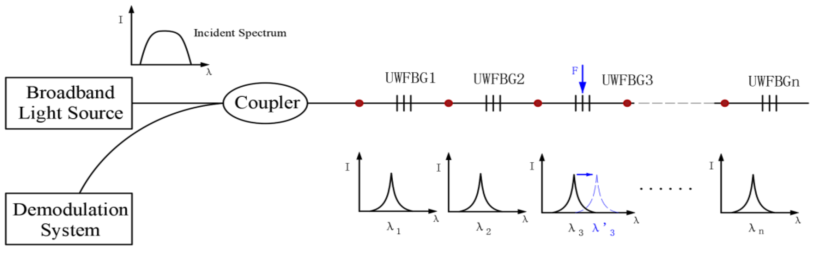
Figure 2.
Basic Concept of the RF Algorithm.
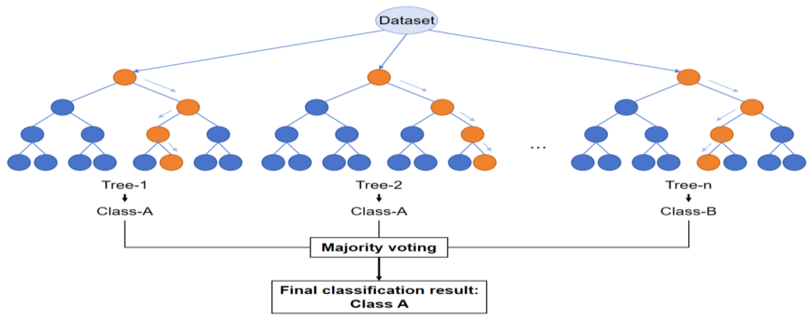
Figure 4.
Principle of the SVM.
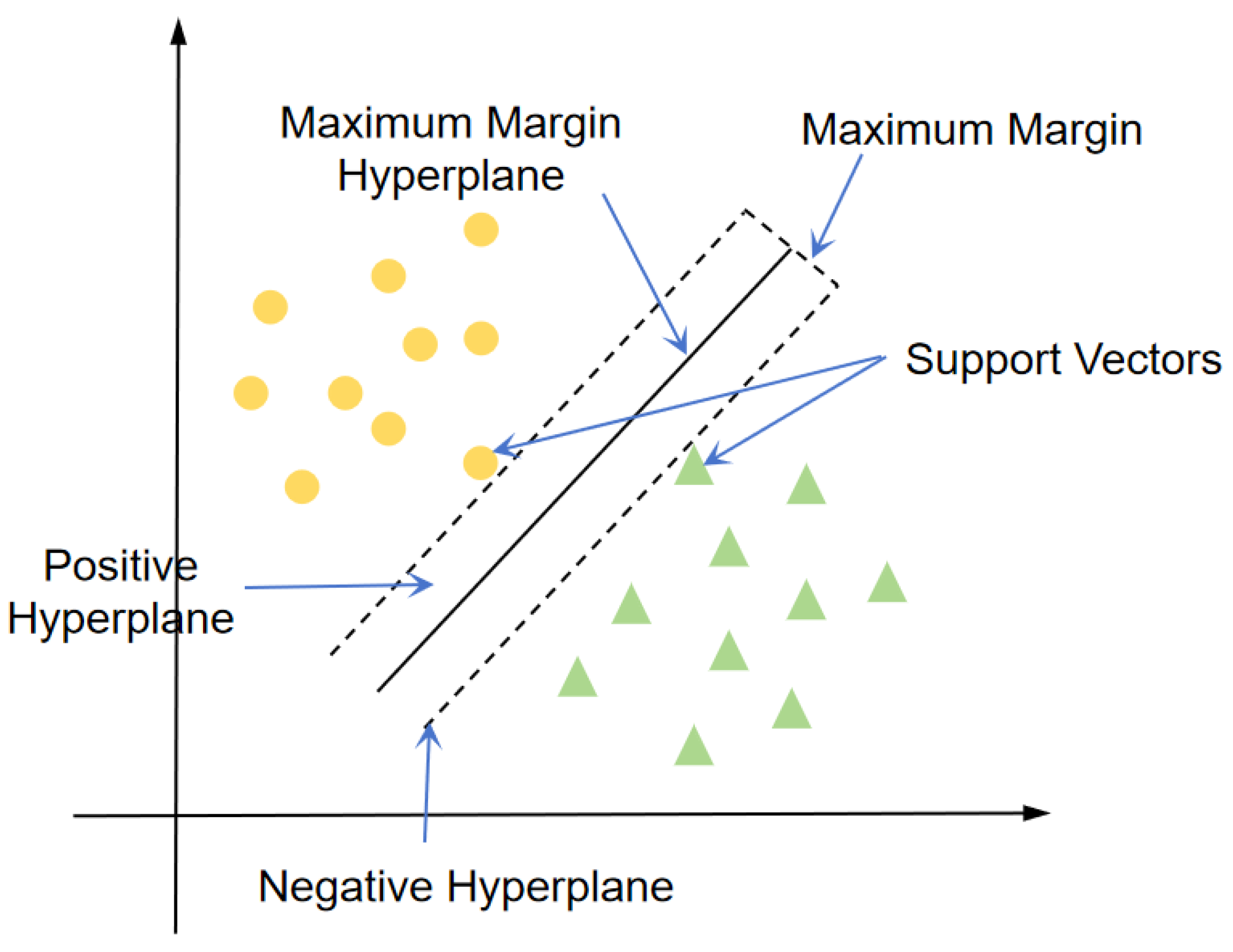
Figure 5.
Cable Deployment on Bridge Deck.
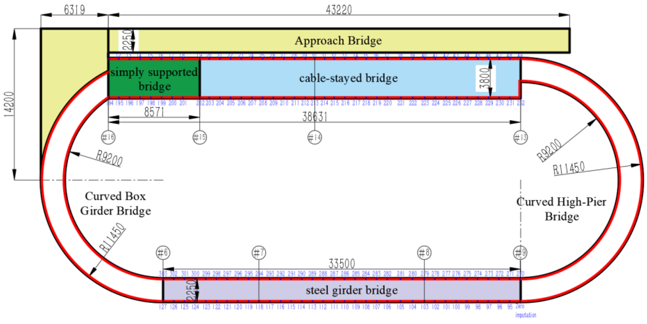
Figure 6.
Cable Deployment on Bridge Underside.
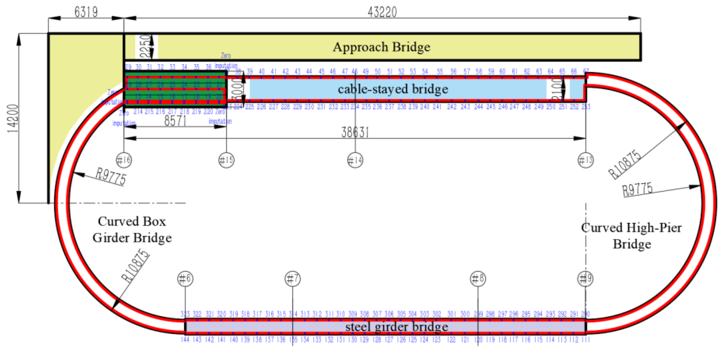
Figure 7.
On-site Layout of Damage Simulation Setups(a) Damage Simulation of Single-slab Loading; (b) Damage Simulation of Eccentric Loading; (c) Damage Simulation of Bearing Detachment.
Figure 7.
On-site Layout of Damage Simulation Setups(a) Damage Simulation of Single-slab Loading; (b) Damage Simulation of Eccentric Loading; (c) Damage Simulation of Bearing Detachment.
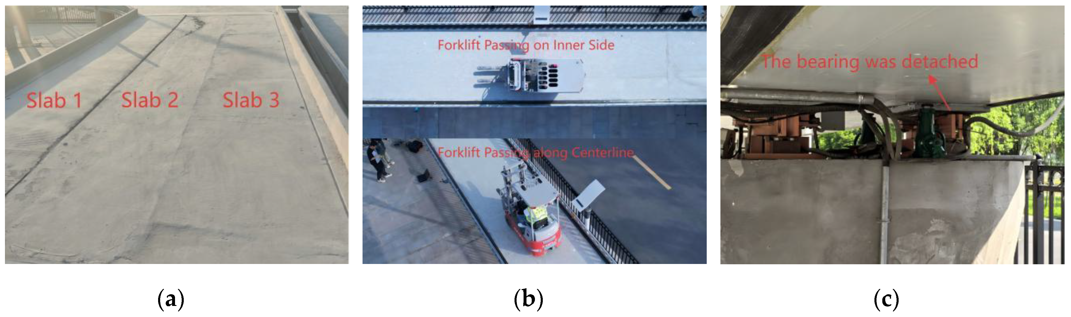
Figure 8.
Flowchart of the Modeling Process for Bridge Structural Defect Identification.
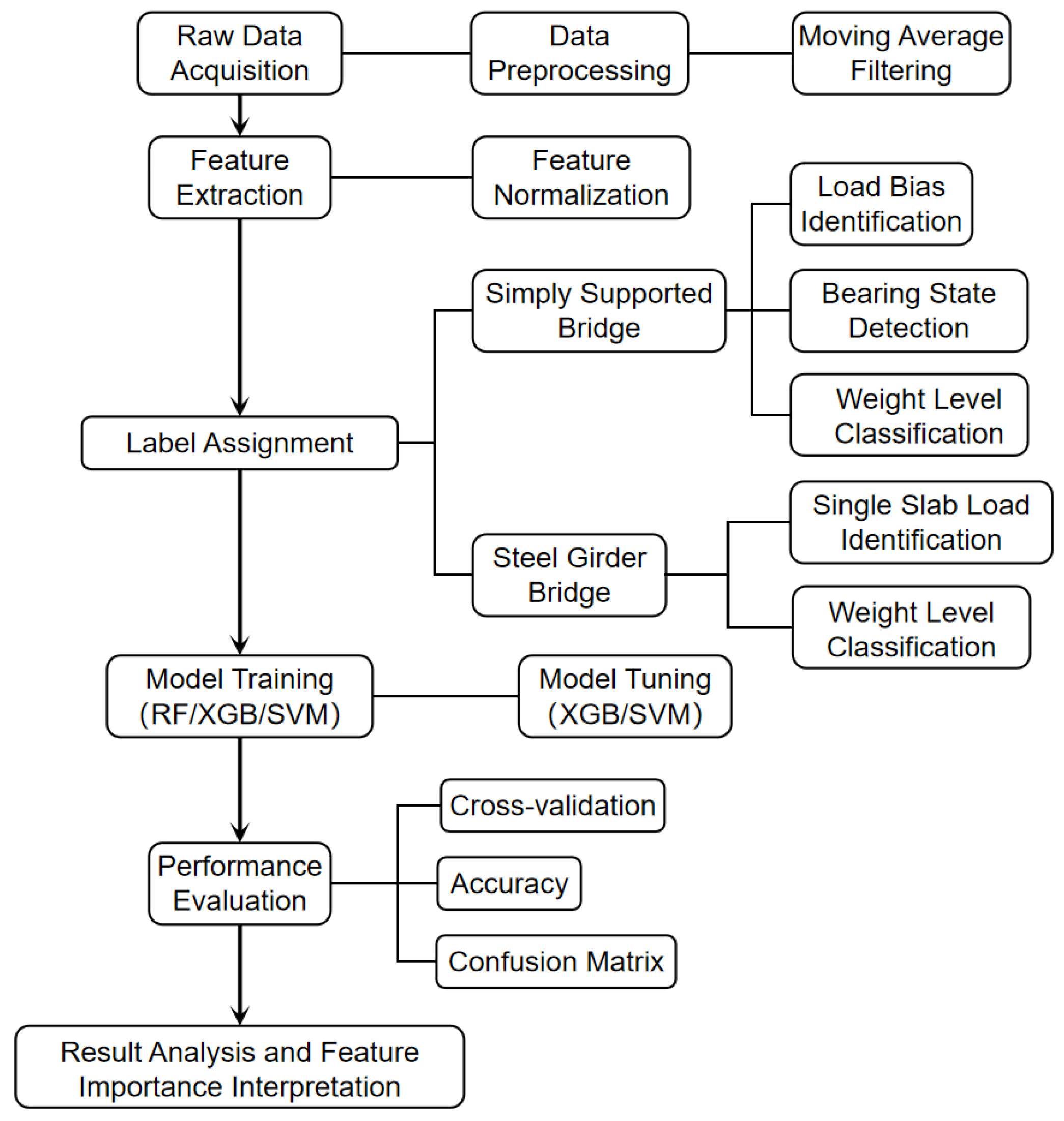
Figure 9.
Confusion Matrix of RF for Single-slab Loading Identification.
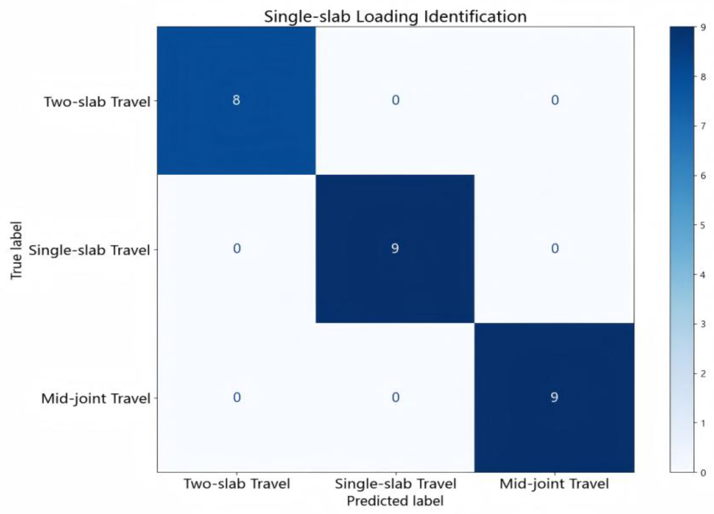
Figure 10.
Confusion Matrix of RF for Eccentric Loading Identification.
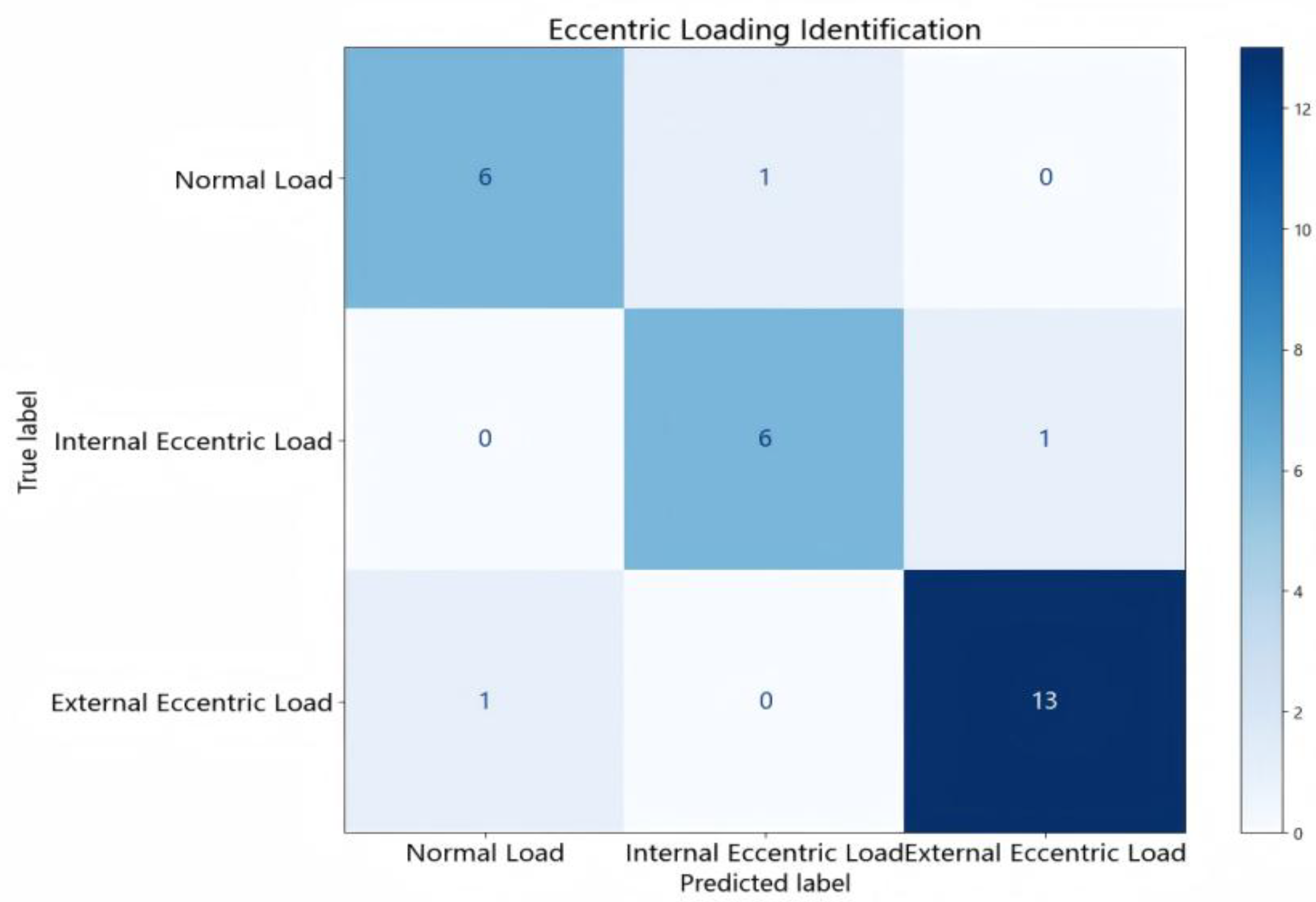
Figure 11.
Confusion Matrix of RF for Bearing Detachment Identification.
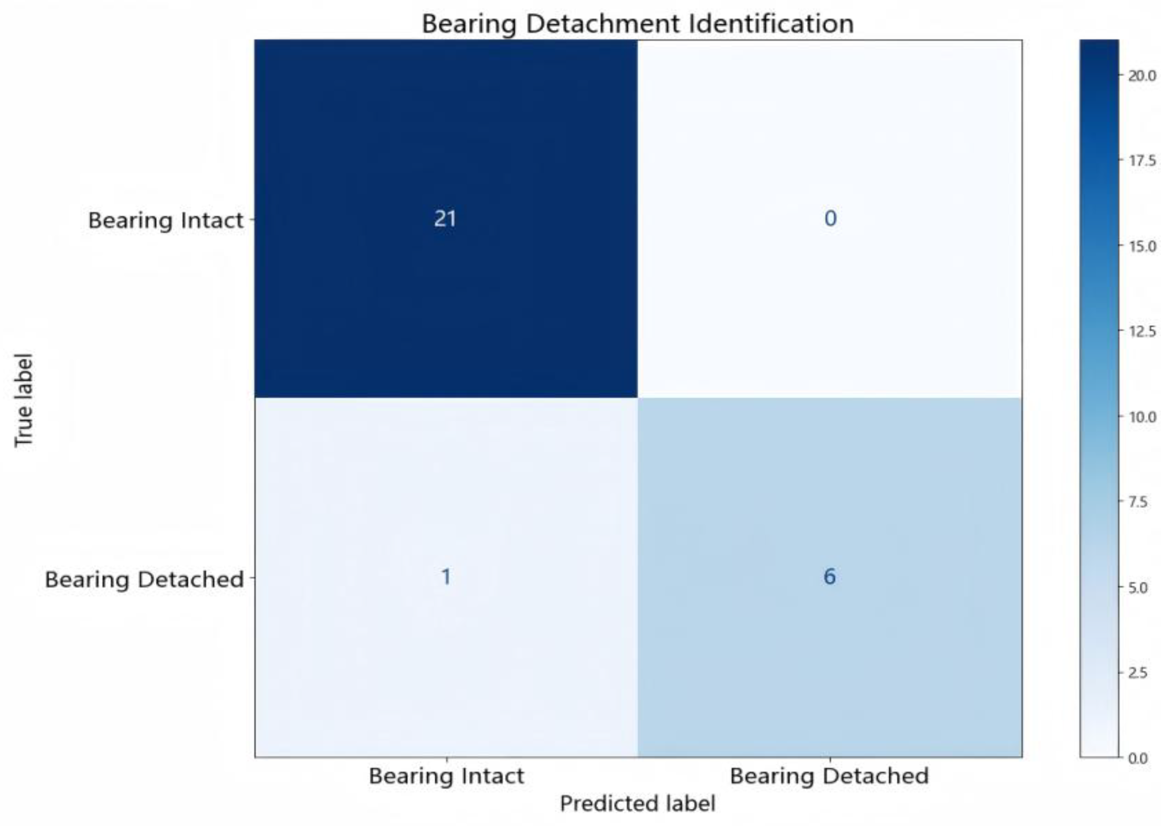
Figure 12.
Confusion Matrix of RF for Weight Level Identification on the Simply Supported Bridge.
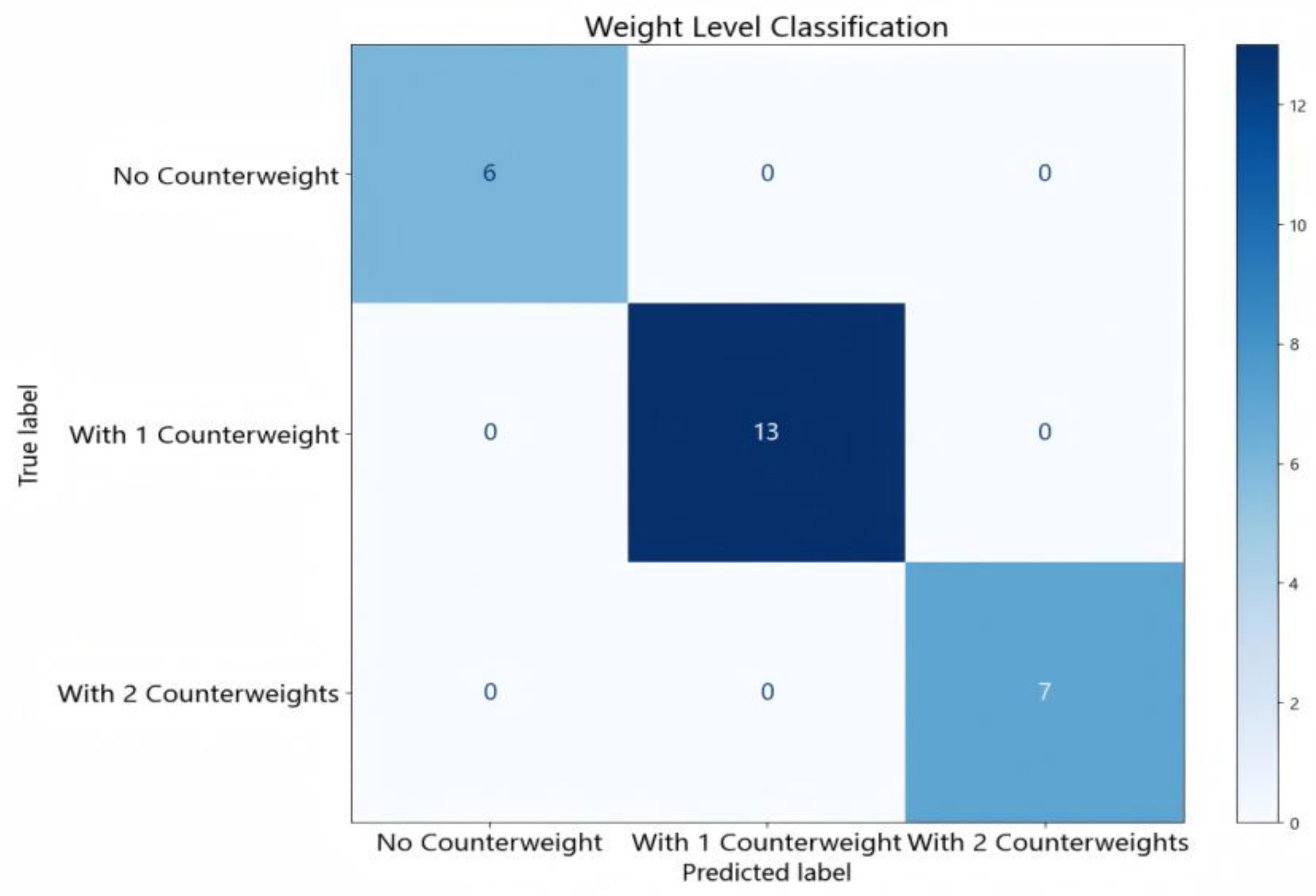
Figure 13.
Confusion Matrix of RF for Weight Level Identification on the Steel Girder Bridge.
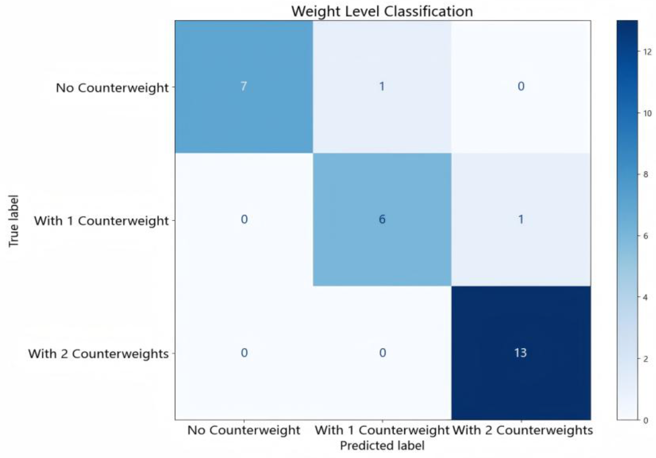
Figure 14.
Feature Importance Ranking for Single-slab Loading Identification.
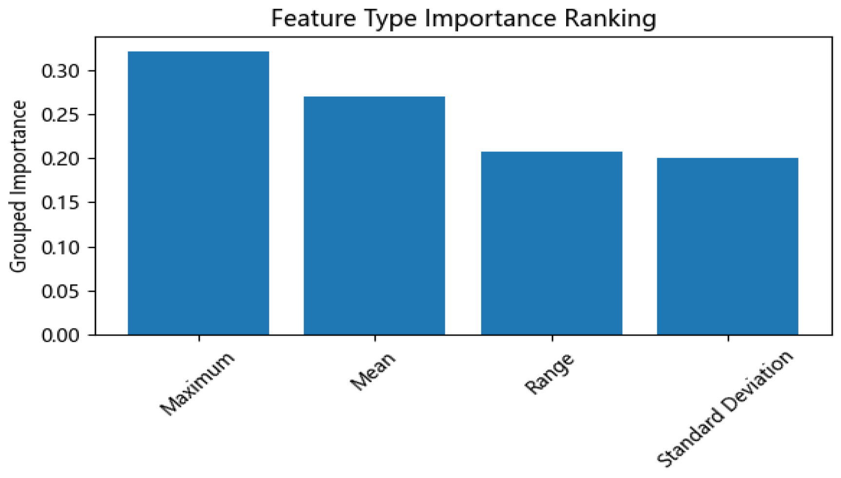
Figure 15.
Feature Importance Ranking(a) Eccentric Loading Identification; (b) Bearing Detachment Identification.
Figure 15.
Feature Importance Ranking(a) Eccentric Loading Identification; (b) Bearing Detachment Identification.
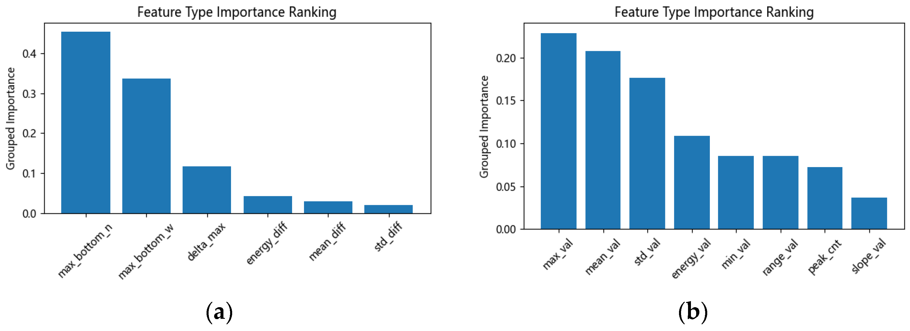
Figure 16.
Feature Importance Ranking for Weight Level Identification(a) Weight Level Identification on the simply supported bridge; (b) Weight Level Identification on the steel girder bridge.
Figure 16.
Feature Importance Ranking for Weight Level Identification(a) Weight Level Identification on the simply supported bridge; (b) Weight Level Identification on the steel girder bridge.
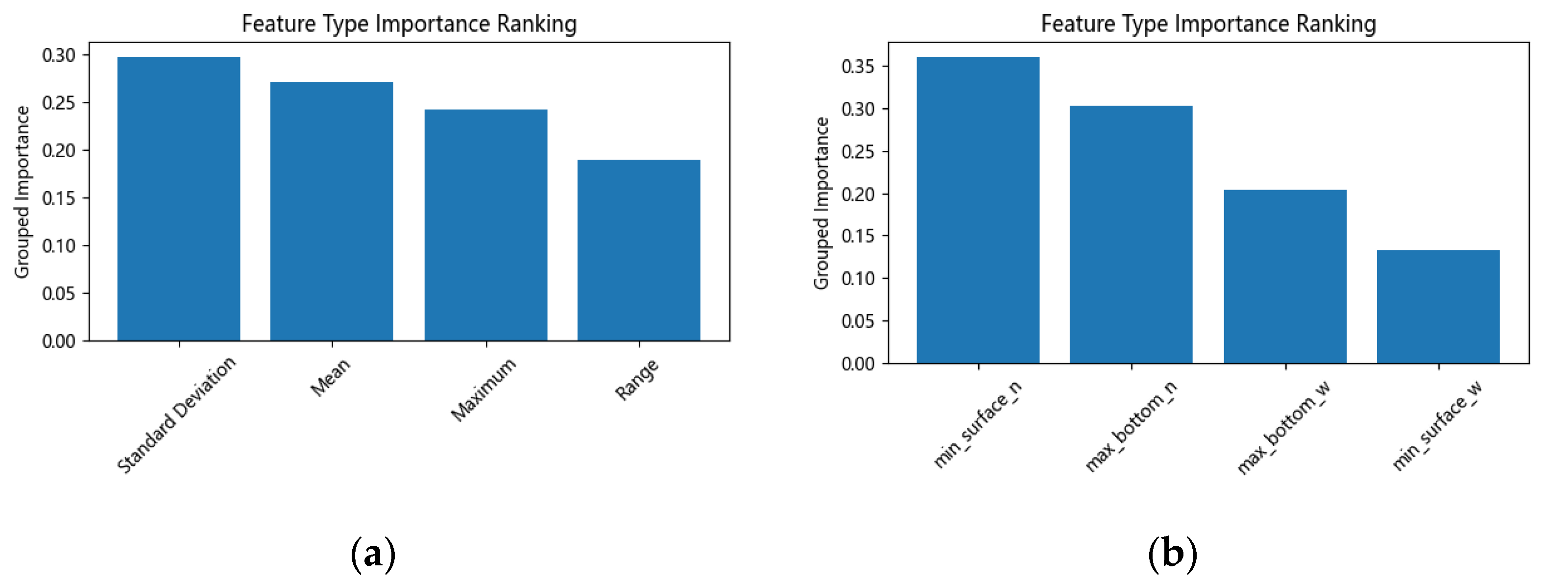

Table 1.
Driving Conditions Table.
| Bridge types | Defect condition |
Driving conditions | Data quantity | |
|---|---|---|---|---|
| Simply supported bridge | Two-slab Travel |
dataOne forklift traveling in the outer lane (No counterweight\ Counterweight 1\ Counterweights 2) | No counterweight: 7 Counterweight 1: 10 Counterweights 2: 10 |
|
| Single-slab Travel |
dataOne forklift traveling in the inner lane (No counterweight\ Counterweight 1\ Counterweights 2) | No counterweight: 10 Counterweight 1: 10 Counterweights 2: 10 |
||
| Mid-joint Travel |
dataOne forklift crossing slab joints (No counterweight\ Counterweight 1\ Counterweights 2) | No counterweight: 10 Counterweight 1: 9 Counterweights 2: 10 |
||
| Steel girder bridge | Eccentric Loading |
One forklift traveling in the middle lane (No counterweight\ Counterweight 1\ Counterweights 2) | No counterweight: 6 Counterweight 1: 8 Counterweights 2: 9 |
|
| One forklift traveling in the inner lane (No counterweight\ Counterweight 1\ Counterweights 2) | No counterweight: 5 Counterweight 1: 9 Counterweights 2: 10 |
|||
| One forklift traveling in the outer lane (No counterweight\ Counterweight 1\ Counterweights 2) | No counterweight: 8 Counterweight 1: 7 Counterweights 2: 9 |
|||
| Bearing Detachment | One forklift traveling in the outer lane (No counterweight) | 5 | ||
| Bearing Detachment at Pier 7 | One forklift traveling in the outer lane (No counterweight\ Counterweight 1\ Counterweights 2) | No counterweight: 5 Counterweight 1: 5 Counterweights 2: 5 |
||
Table 2.
Comparison of Average Classification Accuracies.
| Steel Girder Bridge | Simply Supported Bridge | ||||
|---|---|---|---|---|---|
| Eccentric Loading Identification | Bearing Detachment Identification | Weight Level Identification | Single-slab Load Identification | Weight Level Identification | |
| RF | 0.9205 | 0.9846 | 0.9359 | 0.8333 | 1.0000 |
| XGBoost | 0.7949 | 0.9205 | 0.9359 | 0.8333 | 0.9833 |
| SVM | 0.9026 | 0.9846 | 0.9359 | 0.8500 | 1.0000 |
Table 3.
Evaluation Metrics of RF for Single-slab Loading Identification.
| Precision | Recall | F1-score | Support | |
|---|---|---|---|---|
| Two-slab Travel | 1.00 | 1.00 | 1.00 | 8 |
| Single-slab Travel | 1.00 | 1.00 | 1.00 | 9 |
| Mid-joint Travel | 1.00 | 1.00 | 1.00 | 9 |
| Accuracy | 1.00 | 26 |
Table 4.
Evaluation Metrics of XGBoost and SVM for Single-slab Loading Identification.
| F1-score (XGBoost) | F1-score (SVM) | Support | |
|---|---|---|---|
| Two-slab Travel | 0.94 | 0.78 | 8 |
| Single-slab Travel | 0.89 | 0.82 | 9 |
| Mid-joint Travel | 0.82 | 0.94 | 9 |
| Accuracy | 0.88 | 0.85 | 26 |
Table 5.
Evaluation Metrics of RF for Eccentric Loading Identification.
| Precision | Recall | F1-score | Support | |
|---|---|---|---|---|
| Normal Load | 0.86 | 0.86 | 0.86 | 7 |
| Internal Eccentric Load | 0.86 | 0.86 | 0.86 | 7 |
| External Eccentric Load | 0.93 | 0.93 | 0.93 | 14 |
| Accuracy | 0.89 | 28 |
Table 6.
Evaluation Metrics of XGBoost and SVM for Eccentric Loading Identification.
| F1-score (XGBoost) | F1-score (SVM) | Support | |
|---|---|---|---|
| Normal Load | 0.73 | 0.75 | 7 |
| Internal Eccentric Load | 0.67 | 0.86 | 7 |
| External Eccentric Load | 0.85 | 0.85 | 14 |
| Accuracy | 0.79 | 0.82 | 28 |
Table 7.
Evaluation Metrics of RF for Bearing Detachment Identification.
| Precision | Recall | F1-score | Support | |
|---|---|---|---|---|
| Bearing Intact | 0.95 | 1.00 | 0.98 | 21 |
| Bearing Detached | 1.00 | 0.86 | 0.92 | 7 |
| Accuracy | 0.96 | 28 |
Table 8.
Evaluation Metrics of XGBoost and SVM for Bearing Detachment Identification.
| F1-score (XGBoost) | F1-score (SVM) | Support | |
|---|---|---|---|
| Bearing Intact | 0.95 | 0.98 | 21 |
| Bearing Detached | 0.83 | 0.92 | 7 |
| Accuracy | 0.93 | 0.96 | 28 |
Table 9.
Evaluation Metrics for Weight Level Identification.
| Precision | Recall | F1-score | Support | |
|---|---|---|---|---|
| No counterweight | 1.00 | 1.00 | 1.00 | 6 |
| With 1 Counterweight | 1.00 | 1.00 | 1.00 | 13 |
| With 2 Counterweights | 1.00 | 1.00 | 1.00 | 7 |
| Accuracy | 1.00 | 26 |
Table 10.
Evaluation Metrics of RF for Weight Level Identification.
| Precision | Recall | F1-score | Support | |
|---|---|---|---|---|
| No counterweight | 1.00 | 0.88 | 0.93 | 8 |
| With 1 Counterweight | 0.86 | 0.86 | 0.86 | 7 |
| With 2 Counterweights | 0.93 | 1.00 | 0.96 | 13 |
| Accuracy | 0.93 | 28 |
Table 11.
Evaluation Metrics of XGBoost and SVM for Weight Level Identification.
| F1-score (XGBoost) | F1-score (SVM) | Support | |
|---|---|---|---|
| No counterweight | 0.93 | 0.93 | 8 |
| With 1 Counterweight | 0.75 | 0.78 | 7 |
| With 2 Counterweights | 0.88 | 0.87 | 13 |
| Accuracy | 0.86 | 0.86 | 28 |
Disclaimer/Publisher’s Note: The statements, opinions and data contained in all publications are solely those of the individual author(s) and contributor(s) and not of MDPI and/or the editor(s). MDPI and/or the editor(s) disclaim responsibility for any injury to people or property resulting from any ideas, methods, instructions or products referred to in the content. |
© 2025 by the authors. Licensee MDPI, Basel, Switzerland. This article is an open access article distributed under the terms and conditions of the Creative Commons Attribution (CC BY) license (http://creativecommons.org/licenses/by/4.0/).
Copyright: This open access article is published under a Creative Commons CC BY 4.0 license, which permit the free download, distribution, and reuse, provided that the author and preprint are cited in any reuse.


