
Submitted:
15 June 2025
Posted:
17 June 2025
You are already at the latest version
Abstract
Machine Learning (ML)-based techniques have received significant attention in various fields of industry and science. In civil and bridge engineering, it can facilitate the identification of specific patterns through the analysis of data acquired from Structural Health Monitoring (SHM) systems. To evaluate the prediction capabilities of ML, this study examines the performance of several ML algorithms in estimating the total weight and location of vehicles on a bridge using strain sensing. A novel framework based on combined model and data-driven approach is described, consisting of the establishment of the Finite Element (FE) model, its updating according to load testing results, and data augmentation to facilitate training of selected physics-informed regression models. The article discusses the design of the Fiber Bragg Grating (FBG) sensor-based Bridge Weight-in-Motion (BWIM) system, specifically focusing on several supervised regression models of different architectures. The current work proposes the use of the updated FE model to generate training data and evaluate the accuracy of regression models with possible exclusion of selected input features enabled by the structural specificity of a bridge. The data were sourced from the SHM system installed on a network arch bridge in Wolin, Poland. It confirmed the possibility of establishing the BWIM system based on strain measurements, characterized by an optimized number of sensors and a satisfactory level of accuracy in the estimation of loads, achieved by exploitation of the network arch bridge structural specificity.
Keywords:
artificial intelligence
; machine learning
; neural network
; network arch bridge
; structural health monitoring
1. Introduction
Structural Health Monitoring (SHM) comprises a network of interconnected sensors that are essential elements of the entire monitoring framework [1]. Its establishment may require the integration of various sensor types, each allowing the recording and analysis of specific parameters of structural response. One of the widely used types of sensors is Fiber Optic Sensors which have been successfully applied in many engineering fields, including civil engineering [2,3], geotechnology [4,5], aviation [6], energy [7] and material engineering [8]. They are resistant to corrosion, immune to electromagnetic interference, and versatile in geometric shape [9], while being able to detect small variations in measured values [10].
SHM systems have been increasingly used to estimate road [11,12,13,14] and railway traffic load [15,16,17]. This task, known as Weigh-in-Motion (WIM), or Bridge Weigh-In-Motion (BWIM) specifically for bridge-level load recognition, may involve different methods and instrumentation [18]. The strain-based BWIM systems were developed and introduced for various types of railway bridges, including single-span [19], multi-span [20], and truss structures [21]. The use of specific fiber-optic sensing technologies was reported by Yoon et al. [22] to analyze the response of a bridge superstructure under a train load, allowing identification of car types. Pimentel et al. [23] developed an influence line-based framework to estimate the static axle load, geometry, and speed of trains. Wang et al. [24] proposed the use of crossbeam strain measurement to assess load magnitude using Fiber Bragg Grating (FBG) sensors and the linear superposition algorithm. Although the use of Fiber Optic Sensors in BWIM is apparent, the vast majority of applications involve the measurement of strains in directly loaded components of the railway, including rails, sleepers, and a subgrade [25]. For example, Zhou et al. [26] described the method to estimate the magnitude and positions of the wheel-rail contact forces using Fiber Optic Sensors mounted on the rails. Mishra et al. [27] designed an FBG-based WIM system to estimate train parameters, including the speed, weight, and axle count of cars. Similar characteristics were analyzed by Martincek et al. [28] incorporating the interferometric optical fiber sensing, Lan et al. [29] using the rail- and track slab-embedded sensors, and Mishra et al. [30] who analyzed the impact of train speed and weight on the optomechanical behavior of optical sensors.
In the context of road infrastructure, WIM proposals should address the issues associated with the non-deterministic nature, uncertain positioning, and variety of road traffic scenarios. Reported applications include systems based on the measurement of strains by sensors embedded in a pavement [31,32,33,34] and subgrade layers [35]. Several studies documented the implementation of strain gauges in bridge-level WIM, especially for vehicle detection and classification [36], load magnitude estimation [37], and axle count obtainment [38]. Zhao et al. [39] proposed the framework for axle detection using strain measurement and wavelet transformations. Tan et al. [40] described the detection of vehicle configuration and speed using a strain-based BWIM approach enhanced of the regularization and iterative approach. Similar systems were evaluated considering thermal field effects [41] and spatial variability of structural properties [42]. Heinen et al. [43] examined single-span bridge structures using shear force-based BWIM systems. Among various applications, the use of fiber optic sensing has also been reported. Alamandala et al. [44] proposed a BWIM system using Fiber Bragg Grating (FBG) sensors arranged at different angles. The authors measured wavelength shifts to produce a temporal response curve and predict vehicle parameters, including load and speed. Zhang et al. [45] described a method for assessing vehicle weight considering random traffic flow and using the advantages of long-gauge FBG sensors. Chaudhary et al. [46] proposed an influence line-free BWIM method based on spatiotemporal strain data from Distributed Fiber Optic Sensors (DFOS). The gross weight of the vehicles was identified by spline regression and structural mechanics relationships. Oskoui et al. [47] developed an FBG-based sensor to measure end rotations of a bridge girder for the purpose of estimating vehicle load.
Not many studies have focused on optimizing the layout of the FBG sensors by carefully recognizing the structural specificity of the bridge. In the current research, based on an example of a network arch bridge, it is assumed that the number and location of FBG sensors can be minimized while maintaining the performance and satisfactory accuracy of vehicle weight estimation by exploiting structural specifics of the bridge. The network arch, characterized by inclined hangers that cross each other at least twice, allows a significant reduction in the bending moments for both the arch ribs and the girders, a limitation of the load influence surface range, and a general improvement in structural efficacy compared to other types of arch bridges [48]. However, the difficulties in interpretation of complex traffic conditions with conventional methods have led to an increasing interest in Machine Learning (ML)-based solutions.
Recent advances in computer science have significantly contributed to the enhancement of SHM systems through the integration of ML-based algorithms [49]. These techniques may be used in many areas of civil engineering including damage detection [50,51], estimation of structural deformation [52], and dynamic analysis [53]. ML algorithms are also used in the BWIM approach and their implementation can involve various tools and frameworks. Le et al. [54] proposed the classification approach to detect the structural overload in the railway bridge. Bosso et al. [55] described the regression trees approach to predict vehicle weight and identify the overload trucks. Except for traditional supervised learning, classification and regression models, transfer learning is also often used with very good results. Yan et al. [56] proposed the transfer learning-enhanced CNN algorithm to identify gross weight and axle weight of the vehicles passing the bridge. Their research also showed the possibility of reducing the training set using transfer learning. Also the computer vision is often used in BWIM systems. Jian et al. [57] proposed a BWIM method with a focus on complicated traffic scenarios. Their method can identify strain influence surfaces of the bridge structure and vehicle weights.
The current research integrates the advantages of FBG sensors and ML algorithms for the purpose of SHM system deployment using a network arch bridge in Wolin, Poland, as an example. A novel combined model- and data-driven framework is proposed consisting of the establishment of the FE model, its validation and adjustment based on static and dynamic load testing, and data augmentation to facilitate training of selected physics-informed regression ML models. The work analyses the accuracy and performance of selected ML regression algorithms, namely the Random Forest (RF) and Neural Network (NN), showing the impact of structural specificity of the network arch bridge on the performance of the proposed BWIM system.
Current research is structured as follows. Section 2 presents the bridge and SHM system overview, including details on the arrangement and characteristics of the installed FBG sensors, a description of the network arch-specific strain distribution, and the preparation of training data for the purpose of ML-based BWIM deployment. Section 3 discusses the performance and accuracy of selected ML algorithms in predicting vehicle weight and position for various sets of features. In Section 4, the analysis of uncertainties and evaluation of the proposed ML algorithms are presented. Section 5 contains conclusions, limitations, and perspectives of the developed framework.
2. Methodology
2.1. Bridge and SHM System Overview
The BWIM system, which involves weighing and locating vehicles passing through the structure, was implemented on a steel bridge in Wolin, Poland. The structure is a single-span network arch bridge with a span of 165.0 m. The superstructure consists of two steel arches with a closed box cross section of 1.00 x 1.80 m, connected by steel circular tube bracings of 1.22 m diameter, and slightly inclined inward in relation to the vertical plane. The bridge deck was suspended to the arch ribs with inclined wire hangers arranged in a network layout. The deck has a form of a steel greed structure composed of two longitudinal tie beams and transverse crossbeams placed at a regular spacing of 6.00 m. The distance between the end and the closest middle crossbeams is set at 7.50 m. The cross section of the tie beams is a closed rectangular box measuring 0.75 m in width and 1.30 m in height. The axial spacing between the tie-beams, measured in the transverse cross section, is 16.15 m. The middle crossbeams have an I section of 0.45 m wide and variable height ranged from 0.94 to 1.19 m. The end crossbeams are designed as closed box sections of 2.58 m wide and variable height from 0.88 to 1.20 m. The steel grid is integrally connected to a concrete deck slab, thus forming a composite superstructure. The slab consists of precast concrete slab members interconnected with a 14.0 cm cast in-place layer. The entire steel structure was made of S460N steel, while the bridge slab was made of C50/60 and C40/50 concrete, for precast and in situ layers, respectively.
To estimate the weight and position of the vehicles on the bridge, an SHM system was installed, consisting of optical sensors based on Giber Bragg Grating (FBG) technology. Three measuring gates were designated on the bridge, located at 1/4, 1/2, and 3/4 of the span, in which a total of 17 measuring points were distinguished, based on the response characteristics of the network structure. Each of the measuring gates consists of three points installed on the crossbeam (CB) and two points installed on the hangers (H), one located on the left and the other on the right hanger. The middle gate includes two additional measurement points in the tie-beams (TB), each on one side of the deck.
In the case of the crossbeams and tie-beams, the sensors are spot welded to the structure after prior cleaning and grinding of the surface. In addition to strain sensors, temperature sensors are also installed near the strain measurement points for temperature compensation purposes. The crossbeam sensors are installed on the top surface of the bottom flanges, whereas those on the tie-beams are mounted on the underside of the section. Subsequently, they were protected against corrosion according to the HBK specification [58], including a high adhesion nonhardening masking sealant AK22, 0.05 mm thick aluminum foil coating, and a 3 mm thick layer of kneadable putty, ABM75. The arrangement and characteristics of the welded strain and temperature sensors in the elements of the deck grid are shown in Figure 1.
The hangers installed on the bridge are part of the full locked coil rope system by Teufelberger-Redaelli [59]. These include wire cables of high strength steel that preclude the use of welded strain measurement. Due to the characteristics of the hanger cross-section and the potential torsional effects that may arise in response to the change in tension force, dedicated clamps were fabricated and used for the installation of the strain sensors. They are arranged together with temperature measurement sensors that are attached to the surface of the hanger (Figure 2).
All sensors in the three gates are connected to the breakout cables. These cables extend along the bridge and transmit signals to an MXFS interrogator with 8 inputs of 16 channels each. The Interrogator is installed in a cabinet mounted on one of the bridge end supports. The cabinet is also equipped with an industrial computer for data acquisition, processing, and management, a permanent Internet connection, and an Uninterruptible Power Supply (UPS), which ensures continuous operation in the event of a power outage. The system enables synchronous acquisition from all channels, allowing for time-correlated analysis managed by the CATMAN software. Using the software, it is possible to record in real time the strain values at key points of the structure that will serve as input data for ML-based BWIM algorithms.
2.2. Load Testing and Physics-Informed BWIM Design
After the installation of the sensor system and prior to training of the ML algorithms, load tests were carried out to verify the correct behavior of the structure. Load tests can be an element of the bridge acceptance procedure that confirms design assumptions and allows the estimation of the influence of additional factors on the stiffness and response of the structure. Finally, data obtained on this basis allow verification of the SHM system and calibration of the analytical Finite Element (FE) model, which will ultimately become a source of training data for the purpose of the ML-based BWIM.
The load testing procedure consists of static and dynamic tests. Five different static load schemes were assumed to generate maximum strain values at the selected measurement points. They include three symmetric schemes, one above each of the measurement gates, and two additional asymmetric cases to verify the transverse distribution of loads and the torsional stiffness of the span. The schemes consisted of nine trucks, each of weight between 27.8 and 41.5 t, that were introduced onto the bridge to yield the strain at a level of at least 60% of the theoretical strain values caused by the live load model assumed in the design. According to the established procedure, the load is kept on the bridge for a minimum duration of 30 minutes. The duration of the test is extended by successive 10-minute intervals if strain stabilization has not been achieved. Stabilization is defined as no increase in strain values exceeding 2% between consecutive readings within the 10-minute measurement interval. The response of the structure is also measured after unloading to observe residual strains and to assess the general ability of the structure to return to its initial state.
The data recorded by the SHM system was used to calibrate the numerical FE model, which was then used to generate a synthetic training set for the ML algorithms. Acquiring an appropriate data set solely through experimental studies would entail significant time and financial expenditure, which is why an approach using simulation data was adopted. The main challenge in generating such a set is to ensure its accuracy and reliability in relation to future data observable during the operation of the system in real conditions. This objective was achieved by updating the FE model by modifying the stiffness parameters of its individual components to ensure that the simulated strain values correspond to those observed during load tests. Due to the extensiveness of this subject matter and the constraints on the length of this paper, the current study does not provide a detailed description of the FE model calibration.
In addition to the static load test, the examination of the bridge structure incorporated dynamic tests using a single truck of known weight and dimensions, moving along the bridge. The tests involved passages in different positions on the width of the road, at different speeds, and in different directions, including passing through an artificial obstacle to intensify the vibrations and dynamic response of the bridge. Static and dynamic load tests allowed the identification of the structural specificity of the bridge required for the correct and optimized design of the SHM-based BWIM system. Figure 3 shows the strains measured by three sensors installed on the bottom flange of the crossbeam at the measurement gate no. 3, recorded during one of the dynamic load test passages. The test was carried out using a vehicle with a total weight of 40.6 t, moving at a constant speed of 10 ± 2 km/h. The figure illustrates the timestamps for the entry and exit of the load on the bridge, as well as the timespan that reveals the presence of the vehicle above the gate. The varied intensification of the strains is noticeable within each of the measurement points, which is directly dependent on the position of the vehicle on the width of the road. At the same time, the limited range of the influence surface for strains in the crossbeam is visible, which corresponds to an evident response only for the vehicle located in the immediate vicinity of the monitored beam. The sensors do not detect the presence of a vehicle if the distance is greater than 2 or 3 times the spacing of the intermediate crossbeams, here about 36.0 m. The limited range of the influence surface for crossbeams is an important feature of the network arch bridges compared to structures of different hanger layout. In the context of implementing the BWIM systems, it allows reducing the impact of loads placed over a large part of the bridge, beyond the range of the influence surface. Measurement points on the crossbeams do not require additional processing or filtering to mitigate the influence of other loads in the weight detection procedure for a single vehicle within the gate. At the same time, the system in which weight detection is carried out independently by three successive gates becomes potentially useful, allowing for averaging or cross-validation of the results.
The hangers are characterized by a different shape and range of the influence surface and remain sensitive to the loads outside the gate (Figure 4). In this case, the strains in the hangers recorded during the same test indicate various scales of strain increase depending on the position of the vehicle on the bridge width. Although the timestamp of the maximum strains can also be clearly seen, corresponding to the load located right above the measurement gate, the strain values on the hangers can be affected by other vehicles passing the bridge at a given moment. Considering this specificity and structural behavior of the network arch bridge, the current research attempts to evaluate the performance of various ML algorithms for the purpose of BWIM systems, depending on the set of features considered in the input data.
2.3. Dataset and Machine Learning Algorithms
The entire SHM system can be divided into three main stages: 1) structural monitoring, 2) data analysis using ML algorithms, and 3) bridge management, as seen in Figure 5. In the first stage, Fiber Optic Sensors record the strains in selected points of the structure in real time. These data form the basis for the second stage, in which the applied ML algorithms allow for the prediction of a vehicle weight and position on the bridge, namely the longitudinal and transversal coordinates, X and Y, respectively, based on strain values recorded at selected sensor locations. The ML models are automatically executed on the incoming data and their output is continuously fed into the management layer. The last stage includes the integration of results with infrastructure management systems, such as a digital twin, a dedicated website, and a notification system for exceeding permitted threshold values to enable quick and informed operational decisions. In addition to real-time alerts, all processed data are stored for historical analysis and can be used to assess traffic load trends and structural performance over time.
Figure 6 presents the data flow for the purpose of the ML-based approach incorporated into the SHM system. It consists of the real structure with the installed sensors and the digital FE model that reflects its structural behavior and specifics. The FE model, once updated in the calibration process, is used to generate the training data set. In the current framework, several regression ML algorithms of various architectures and number of inputs are evaluated and compared in terms of precision in predicting vehicle weight and coordinates. The best-performance model can be utilized to establish a BWIM module in the final system, wherein continuous sensor readings are used to collect information about road traffic and load magnitude on the bridge.
To automate the generation of data sets for the training and validation of regression ML algorithms, a dedicated framework was developed, allowing direct use of the updated FE model (Figure 7). The model was created in SOFiSTiK software, a commercial structural analysis environment, using text batch files with the content defined in the internal CADINP language and the SOFiSTiK API adapted to the object-oriented C# programming language. The code includes methods responsible for reading the batch files with the definition of geometry, materials, and load cases, calculation, and saving the strain results to an Excel workbook. In the loadings, sets of concentrated forces corresponding to the axle arrangement of seven typical truck vehicles were provided, including those used in the load tests. The vehicles were located in different positions on the bridge and assigned different total weights, while maintaining the proportion of load distribution on the individual axles. The diversity of vehicles will allow the assessment of the universality of the ML models in predicting the total weights of vehicles with different numbers and axle spacings.
The objective of the study is to determine the ability of ML algorithms to predict the position and weight of vehicles based on the strains. Therefore, the defined task is a multivariate regression, in which the maximum number of variables equal to the total number of strain sensors installed on the bridge may be exploited, here 17. In addition, the gradual reduction of input features and its impact on the accuracy of the prediction are analyzed. Three ML models of various architectures and number of inputs are trained and compared: Random Forest (RF), including its variant of the single-ensemble Decision Tree (DT), and Neural Networks (NN).
A synthetic data set of 6 000 samples was generated and divided into training and test sets of sizes 4 800 and 1 200, respectively. The input features consist of strain values, and the output includes the coordinates and weight of the vehicle. The accuracy of each regression model was evaluated using the Root Mean Square Error (RMSE) as the primary metric. The same input structure was used for all algorithms to compare their predictive accuracy.
Where:
– number of elements in the data set,
– matrix containing the values of all features (excluding target values) of all samples,
– vector of feature values (excluding target values) of the ith sample,
– target value of the ith sample,
– model’s prediction function.
3. Results
3.1. Random Forest-Based Predictive Models
The Random Forest (RF) is one of the ensemble ML algorithms used in various classification and regression tasks. For the latter, it consists of a given number of regression decision trees, each of which is independently trained on a specified group of samples from the training set. The training process consists of gradually expanding the tree by splitting the set into two nodes. Newly created nodes are progressively split into deeper subsets until a stop criterion is met, usually reaching the maximum tree depth or minimum number of samples in the node. In the current approach, the best split in the node is obtained by minimizing the average squared difference between the feature values of the samples assigned to the potential subnodes and their means. The splitting algorithm evaluates every possible split and selects the one that results in the greatest reduction in mean squared error in the resulting subsets. This process is repeated for a given and subsequent nodes until a single element leaves at the end. A single RF consists of several decision trees, making the model more diverse and reducing the variance of the entire forest. The final prediction is calculated as the average of the outputs returned by each of the trees.
In the current study, RF models of different number of decision trees and different number of training samples in relation to the size of the whole dataset are considered and compared with the performance of the NN regression models. At first, different RF architectures are trained on the strain values recorded by all sensors in the system at a specific timestamp. The performance of the regression model is analyzed by the RMSE value of the predictions on the weight and transverse position of the vehicle, Y. As seen in Figure 3 for the strains in the crossbeam, the exact timestamp that triggers the predictions, as well as the longitudinal placement of the load, X, can be clearly indicated by the peak values in the strain time series data.
Figure 8 and Figure 9 show the impact of the RF architecture on the prediction error for vehicle weight and its transverse position, Y, respectively. Five various numbers of trees are assumed, in turn 1, 10, 50, 100, and 500 trees. For each number, different relative sizes of the training subsets are analyzed, labeled as max samples, and ranging from 10.0 to 100.0%. The models are evaluated on training and test sets to estimate the variance and assess the ability of the model to generalize the results for inputs that did not participate in the learning process.
For single-tree architectures, the RMSE values are in the range of 166.0 to 372.6 kg for weight and 0.116 to 0.297 m for coordinate Y. The variance of a single decision tree is regularized by the introduction of sampling with replacement, which allows for repetitive occurrence of samples in the training subset, while keeping some of the samples out of the badge. In most cases an effect of overfitting is observed in which the error measured on the test set is higher than the error on the training set. The problem can potentially be solved by introducing more trees or using additional regularization techniques, including reducing the size of the training subsets. The overfitting effect is reduced only for drastically reduced subsets, at least 25.0.% of the initial set size. Despite the effect, the best performance model is usually chosen based on the error measured on the test set. Following this assumption, it can be seen that the higher the number of tress and the larger the size of the subset, the higher the accuracy of the RF model. For models consisting of at least 50 trees and trained on at least 75.0% of the initial set, the accuracy measured on the test samples lies in the range of 111.8 kg to 114.4 kg for total weight and 0.038 to 0.043 m for Y estimations. It is possible to achieve an accuracy of less than 50.0 kg for the training set.
Reducing the features set by excluding the strains measured at the points outside the given measurement gate allows limiting the potential impact of vehicles located in other parts of the bridge. In this case, a 5-element input vector is considered consisting of strain points on the crossbeams and two hangers on the left and right sides of the deck. On the example of the gate no. 1, the accuracy of the weight and transverse position predictions decreases for all RF architectures considered, as shown in Figure 10 and Figure 11. For the best model identified for the entire set of features, the RMSE value measured for the test set drops from 111.8 kg to 391.9 kg, which is still satisfactory considering the expected traffic load range of estimated up to 40 t. The achievable accuracy for the prediction of the transverse position reaches 0.070 m.
Further reduction of features in the input vector may involve excluding strains in hangers while maintaining the strain reading in the measurement gate crossbeam. In this case, due to the limited range of the influence surface, the RF input values depend only on the vehicles located within the gate and its closest vicinity. This approach allows for exclusion of the use of algorithms that filter the influence of distant loads, which, however, involves further reduction in the accuracy in predicting weight and transverse position. The RMSE measured in the training and test set for the 3-input vectors for the same RF architectures are shown in Figure 12 and Figure 13. For the best model identified so far, the RMSE value measured for the test set drops to 1 266.7 kg, which is significantly lower than the required level of accuracy assumed in the specification, 0.5 t. The RMSE for the transverse position is less than 0.130 m.
It was also noted that the performance and accuracy of the RF models depend to a large extent on the size of the training set. With 4,800 samples in the training set, the learning time of a 500-tree 3-input RF model was within 6 seconds, which is much shorter compared to the time required to train more advanced models, including neural networks. As seen in Table 1, a tenfold increase in the size of the training set allows a reduction of the RMSE value in weight prediction to an acceptable level of 509.6 kg with an increase in training time to 73.2 s.
3.2. Neural Network-Based Predictive Models
In this research, which consists of the prediction of the weight and location of the vehicles passing by the bridge, Neural Network (NN) models can also be used. This is an example of a regression problem, in which NN have high accuracy and effectiveness. These models are used for complex predictions and identification of dependencies between input and output data. Under their assumption, they constitute a network of interconnected neurons grouped into input, output, and intermediate hidden layers. All input data are transferred to the first layer of the network and then transformed into subsequent layers according to the assigned weights. The value stored in each neuron corresponds to the sum of the products of the values from neurons from the previous layer and the weights assigned to each connection. Then it is modified by adding an additional deviation and transformed using an activation function. In practice, the operation of NN can be described using a matrix equation that transforms the input data. During the training phase, the NN adjusts the model weights for each connection to the most closely represent the known output given the input.
When designing NN, an important part is the selection of the appropriate architecture, in particular, the number of layers and neurons. In the presented study, a total of 25 different NN architectures were tested, including configurations with 1, 2, 3, 5 and 10 hidden layers and with 10, 50, 100, 150 and 200 neurons in each layer. The NN were tasked with accurately prediction of the location of the vehicle on the bridge in the transverse Y direction and its weight. Each of the networks was trained for a maximum of 1000 epochs, using an early stopping mechanism with the patience parameter set to 100 epochs. During NN training, the learning rate plays a very important role, defining the size of parameter changes in each iteration. Too high a value can lead to learning instability, where the model weights tend to infinity instead of stabilizing. On the other hand, too low a value leads to slow convergence and creates the risk of stopping the learning process at a local minimum. Therefore, different learning rate values were tested, finally choosing the value for which the best models were obtained. The values of 0.001, 0.005, 0.01, 0.05 and 0.1 were adopted. The loss function was the Huber function, which combines the features of the Mean Square Error (MSE) and the Mean Absolute Error (MAE). For small errors (below the threshold value), it has a quadratic character, making it learn faster and achieving convergence near the target values. However, above the threshold value, it takes a linear form, which makes it more resistant to outliers. The metric defining the accuracy of each architecture was the Root Mean Square Error (RMSE) calculated for the entire training and test set (Figure 14 and Figure 15).
For vehicle weight prediction, the best accuracy is achieved by NN of moderate depth consisting of 2 or 3 hidden layers. Shallower networks with 1 hidden layer are not able to correctly model the relationships between data, achieving significantly higher RMSE error values. There is also a noticeable decrease in accuracy for deeper networks with 5 or 10 layers, leading to higher RMSE values. The best accuracy was achieved for NN consisting of 2 hidden layers and 100 neurons, for which the RMSE error is 19.9. The predictions presented for 17 input data show that increasing the depth and number of network neurons will not necessarily lead to better accuracy. Choosing an architecture consisting of 2 or 3 hidden layers with at least 50 neurons will be the best compromise between model accuracy and its complexity.
For prediction of the Y coordinate of a vehicle on a bridge, the best results are achieved by NN with a depth of 2 to 10 hidden layers. Shallow networks or those containing a smaller number of neurons were characterized by greater overfitting, resulting in higher RMSE error values in the test set compared to the training set. This indicates the inability of simpler models to capture complex dependencies between data. In turn, networks with a larger number of layers did not provide further improvement in accuracy and achieved RMSE error values similar to those of simpler two- or three-layer networks. The best accuracy was obtained for a network consisting of 5 hidden layers and 150 neurons, achieving an RMSE error of 0.017 and the lowest degree of overfitting in relation to all architectures. However, two-layer networks with 50 or more neurons achieve satisfactory results and can be a good compromise between accuracy and model complexity.
In the case described above, the input data are the strains recorded on all 17 sensors. In such a system, it may be difficult for the NN to determine the location of the vehicle in the longitudinal direction X when there are more vehicles on the bridge at the same time. This results from the specificity of the operation of the arch structure with a network suspension, which is characterized by small areas of influence for the measurement points located on the crossbeams. They cover only about two bands of crossbeams, which means that they record strains only when the vehicle is directly above a given measurement gate. Consequently, when there are more vehicles on the bridge, the NN may have difficulty accurately predicting the exact weight and location of each of them. For this reason, it was decided to use measurement gates as an effective method to determine the position of the vehicle along the length of the bridge because the results obtained will not be disturbed by vehicles standing at a greater distance from a specific gate. Therefore, NN can predict the position Y and the weight of only one vehicle at a time, currently passing through the measurement gate. As a result, it can be assumed that the X coordinate of the vehicle position is equal to the position of the measuring gate along the bridge.
NN were trained with input data collected from a single measurement gate consisting of five sensors, located on crossbeams and hangers. The same architectures were analyzed as for 17 input data, consisting of 1, 2, 3, 5, and 10 hidden layers and 10, 50, 100, 150, and 200 neurons, respectively. Each network was trained for a maximum of 1000 epochs, assuming an early stopping mechanism with a patience factor of 100 and analyzing different values of the learning rate, 0.001, 0.005, 0.01, 0.05, and 0.1, respectively, choosing the value for which the model performed best. The RMSE error values were then determined for the training and test sets (Figure 16 and Figure 17).
In the case of weight prediction with 5 input data, networks with at least two hidden layers and 50 neurons perform very well, achieving RMSE error values below 100. On the other hand, the shallow network with one hidden layer is too simple and was unable to effectively model the appropriate relationship between data for any learning rate. These networks (except for the one with 150 neurons) stopped at a local minimum and were unable to fully carry out the learning process. Their training was stopped already around the 300th epoch using the early stopping mechanism, which indicates that they did not improve their accuracy during the subsequent epochs. There is also a slight increase in the RMSE error values for more complex architectures, including 10-layer networks, which achieve RMSE errors exceeding 100. The best accuracy was achieved by the NN with 5 hidden layers and 100 neurons, for which the RMSE error is equal to 68.0.
The best accuracy in determining the vehicle Y coordinate is achieved by networks with at least 3 hidden layers and 50 neurons. There is also a slight improvement in accuracy compared to networks using all 17 input data. Also in this case, increasing the depth of the network does not lead to achieving better accuracy, and networks with 3 or 5 hidden layers are good solutions, which are also not complex architectures. The best accuracy was achieved by a network with 5 hidden layers and 150 neurons, for which the RMSE error value is 0.013.
The disadvantage of the models using 5 inputs is the consideration of strains from the hangers. Although the influence surface for the crossbeams is rather limited and covers a narrow range, for the hangers it reaches much further along the bridge. As a result, with a larger number of vehicles, the effectiveness of these models can be disturbed by vehicles standing in front of or behind the measuring gate. Further data filtering and NN training show a greater influence of the model architecture on its accuracy. In this case, the RMSE error values are larger than in the previous models, but they will not be disturbed by other vehicles that are not located above the specific measuring gate. At the same time, the accuracy achieved by these networks is sufficient in the conducted study (Figure 18 and Figure 19).
In the case of vehicle weight prediction, NN with at least 2 hidden layers and 50 neurons performed very well, being able to make predictions with an accuracy of about 200 kg, which is sufficient for vehicles weighing up to 40 t. Shallow networks with 1 hidden layer and a small number of neurons were too simple and were unable to correctly complete the learning process, stopping each time at a local minimum, while checking different variants of the learning rate. Three-layer networks provide a good compromise between accuracy and model complexity and can be successfully used in vehicle weight prediction. On the other hand, the best accuracy was achieved by NN with 10 hidden layers and 50 neurons, for which the RMSE error value is 186.2.
The RMSE error for predicting the Y coordinate of the vehicle’s position decreases with the increase in the number of neurons in the network layers. However, for NN with at least 3 hidden layers and 50 neurons, they already reach similar values that constitute good solutions, with not necessarily complicated architectures. On the other hand, shallower networks, especially those with 1 hidden layer, do not generalize new data well and perform much worse, achieving about twice as high RMSE error values and being characterized by slight model overfitting. The best accuracy is characterized by a network with 5 hidden layers and 100 neurons, which reached an RMSE error value of 0.036.
4. Measurement Uncertainties
Although the use of various type of sensors and ML models provides high accuracy, this system is not free from measurements uncertainties. They can be divided into two main groups based on their origin: 1) resulting from technological limitation of the installed sensors; 2) resulting from limitation and assumptions made in ML algorithms. The error in predicting new values can be estimated using one of available methods: the criterion of correct prediction or a regression model.
4.1. Criterion of Correct Prediction
The error of the predicted target values is estimated using the criterion of a correct prediction [60], which is determined by the condition (Equation (3)):
Where:
– comparison error,
– prediction uncertainties.
The comparison error is calculated as the difference between the experimental error and the generalization error (Equation (4)).
Where:
– experimental error,
– generalization error.
The experimental error results from the installed sensors, while the generalization error concerns the used ML model. It is based on two main components – the error resulting from incorrectly adopted model assumptions (bias error) and the accuracy of the model – in the presented system, the RMSE (Equation (5)).
Where:
– experimental error,
– generalization error.
The value of the prediction uncertainty is determined by the Equation 6.
Where:
– experimental uncertainty,
– data uncertainty,
– fitting uncertainty.
4.2. Regression Model to Estimate Uncertainties
The second method of estimating the error in predicting new values is based on a regression model (Figure 20) defined by Equation 7.
Where:
, – structural parameters of the function,
– random component.
The regression model is implemented in this research to check the accuracy of the ML algorithms. Perfect fitting occurs when the error is equal to 0, meaning the regression model takes the form . In this regression model, is a coefficient indicating the deviation of the predicted results from the measurement. The average difference (standard error of estimate) between measured and predicted values is the simulated error; where is the variance of the model residual.
Therefore is a benchmark of model fit, based on the model residual – the discrepancies between the actual values of the dependent variable in the sample and the value of the convergent dependent variable calculated on the basis of the model. Therefore, the goal is to achieve a situation where the variance value tends to 0: . Figure 21 presents the regression models obtained from the best performing models predicting the vehicle weight based on three input data. These models are: an NN with 10 hidden layers and 50 neurons per layer, and a RF consisting of 100 trees with the tree size built by sampling with replacement and the size equal to the initial set.
5. Conclusions
The article presents the implementation of the BWIM framework based on fiber optic sensors and FBG technology. Its design integrates the data obtained from the SHM system and ML algorithms that allow the prediction of the total weight and position of vehicles on a network arch bridge. To generate a training set, a load test of the bridge was carried out, during which strains measured by the fiber optic sensors were recorded. The strain measurement points were placed at key points of the structure to ensure an accurate representation of its response and operation. Based on these load tests, the FE model updating procedure was performed, which is an important step in the process of building the entire system based on fiber optic sensors and ML algorithms. Thanks to it, it is possible to generate a training set and assess the impact of the specificity of the bridge structure on the final operation of the BWIM system.
Based on the analyses carried out, it was shown that reducing the number of sensors and focusing on specific measurement gates to predict vehicle weight and location eliminates the influence of other loads on the bridge. This is caused by the specifics of the network arch bridge, in which the points located on the crossbeams are characterized by small influence surfaces. Due to this, each of the sensors records the impact of a vehicle located in close proximity to the measurement gate, and its indications are not disturbed by other loads and vehicles located at a further distance.
In order to predict the total weight and position of vehicles on the bridge, the accuracy achieved for the Random Forest (RF) and Neural Network (NN) models was compared. Various hyperparameters and architectures with significant impact on the learning process were taken into account. The first group of ML models investigated comprises RFs as an example of the ensemble learning methodology. It consists of a set of decision trees, each of which is trained on a different subset of the training set. The training is much shorter than that of NN and involves a smaller number of hyperparameters, mainly regularization operators, but requires a comparatively large number of training samples to achieve the assumed accuracy. In this study, after reducing the number of sensors and training the model on three input features, namely the crossbeam strains within a single measurement gate, the accuracy achieved for the architecture consisting of 500 trees is about 1.3 t and 0.5 for 4 800 samples and 48 000 samples in the training set, respectively. Increasing the number of decision trees, as well as increasing the size of the subsets used to train individual trees, improves performance, both on the training and test sets. However, these models experience overfitting, obtaining much better RMSE values in the training data compared to the test set. The necessity of increasing the size of the training set further proves the usefulness of the proposed procedure in which the FE is calibrated based on the load tests and then used in the establishment of BWIM based on ML. This allows the replacement of time- and resource-consuming site experiments with FE simulation for the purpose of generating training and test sets.
To achieve better accuracy and reduce the effect of overfitting, NN models were introduced into the system. Various architectures were analyzed, including the number of layers and neurons. On the basis of the obtained results, it was found that a deeper and more complex NN does not necessarily give better results. Often, good correspondences can be obtained for a moderate depth consisting of 2-3 hidden layers and about 50-100 neurons. This solution provides a good compromise between the accuracy of the model and its complexity, which significantly affects the computation time. However, shallow networks consisting of only one hidden layer are often too simple to model complex dependencies in the data and are also susceptible to overfitting. Due to their simplicity, they can often have a problem in the training phase and will stop at a local minimum that is not an optimal solution. In addition, a significant influence of the learning rate on the learning process of NN was identified. Therefore, it was decided to analyze different values for each of the architectures. Its inappropriate selection can cause instability in the learning process and lack of stabilization in the selection of model weights, or slowing down and stopping at a local minimum that may be far from the optimal solution. Similarly to RF, the best results were achieved when 17 sensors were used as input data. The gradual reduction of features slightly worsened the accuracy of the model, finally achieving about 200 kg for three input data. Despite the higher error value compared to the training models on the full set of input features, the accuracy is sufficient from the point of view of the target application, in which the expected load intensity reaches the order of 30 - 40 t. When the number of features in the input data is reduced, the influence of other vehicles located outside the area of influence of the crossbeam gates is eliminated.
However, the methodology presented has certain limitations that require further research. Fiber optic sensors installed to the structural elements and hangers did not allow the axles to be distinguished from passing vehicles, making it impossible to determine the exact type of vehicle. Therefore, in the current approach, it is not possible to determine the load on each axle, but an appropriate sensor arrangement provides good accuracy to predict the total weight of the vehicle. Furthermore, the presented research focused on the occurrence of one vehicle within the measurement gate. The surface of influence for which the sensors register the vehicle is approximately twice the crossbeam spacing, i.e. approximately 12 meters. A situation in which two or more vehicles are simultaneously in this area of the bridge, if it is relatively rare, requires appropriate preparation and calibration.
Based on the analyses conducted, directions for further work and possible research can be determined, which include the generation of a Digital Twin (DT) based on sensors and the SHM system. Reducing the number of sensors for the prediction of vehicle weight and location not only optimized the entire system, but also created a framework for the construction of a DT model. Due to the prediction of vehicle weight and location determined on the basis of a limited number of sensors reading, it is possible to simulate load effects and compare them between the FE model and the remaining sensors. A system constructed in this way provides the possibility of full automation of the structural monitoring and anomaly detection system, in which the basic elements, in addition to the ML algorithms, are installed fiber optic sensors.
Author Contributions
Conceptualization, D.P., M.J. and S.P.; methodology, D.P., M.J., A.N., P.L. and S.P.; software, D.P. and M.J.; validation, D.P. and M.J.; formal analysis, D.P. and M.J.; investigation, D.P., M.J., A.N., P.L. and S.P.; resources, P.L.; data curation, S.P.; writing—original draft preparation, D.P., M.J., A.N. and P.L.; writing—review and editing, D.P., M.J., A.N. and P.L.; visualization, D.P. and M.J.; supervision, A.N. and P.L.; project administration, A.N., P.L. and S.P.; funding acquisition, S.P. All authors have read and agreed to the published version of the manuscript.
Funding
This research received no external funding.
Institutional Review Board Statement
Not applicable.
Informed Consent Statement
Not applicable.
Data Availability Statement
On request from the authors.
Conflicts of Interest
The authors declare no conflict of interest.
References
- Pozo, F.; Tibaduiza, D.A.; Vidal, Y. Sensors for Structural Health Monitoring and Condition Monitoring. Sensors 2021, 21, 1558. [Google Scholar] [CrossRef] [PubMed]
- Moser, D.; Martin-Candilejo, A.; Cueto-Felgueroso, L.; Santillán, D. Use of Fiber-Optic Sensors to Monitor Concrete Dams: Recent Breakthroughs and New Opportunities. Structures 2024, 67, 106968. [Google Scholar] [CrossRef]
- Richter, B.; Messerer, D.; Herbers, M.; Speck, K.; Laukner, J.; Gläser, C.; Jesse, F.; Marx, S. Monitoring of a Prestressed Bridge Girder with Integrated Distributed Fiber Optic Sensors. Procedia Structural Integrity 2024, 64, 1208–1215. [Google Scholar] [CrossRef]
- Li, H.-J.; Zhu, H.-H.; Wu, H.-Y.; Zhu, B.; Shi, B. Experimental Investigation on Pipe-Soil Interaction Due to Ground Subsidence via High-Resolution Fiber Optic Sensing. Tunnelling and Underground Space Technology 2022, 127, 104586. [Google Scholar] [CrossRef]
- Ren, B.; Zhu, H.; Shen, Y.; Zhou, X.; Zhao, T. Deformation Monitoring of Ultra-Deep Foundation Excavation Using Distributed Fiber Optic Sensors. IOP Conf Ser Earth Environ Sci 2021, 861, 072057. [Google Scholar] [CrossRef]
- García, I.; Zubia, J.; Durana, G.; Aldabaldetreku, G.; Illarramendi, M.; Villatoro, J. Optical Fiber Sensors for Aircraft Structural Health Monitoring. Sensors 2015, 15, 15494–15519. [Google Scholar] [CrossRef]
- Bae, C.; Manandhar, A.; Kiesel, P.; Raghavan, A. Monitoring the Strain Evolution of Lithium-Ion Battery Electrodes Using an Optical Fiber Bragg Grating Sensor. Energy Technology 2016, 4, 851–855. [Google Scholar] [CrossRef]
- Ikeda, Y.; Takeda, S.; Hisada, S.; Ogasawara, T. Detection of Matrix Cracks in Composite Laminates Using Embedded Fiber-Optic Distributed Strain Sensing. Sens Actuators A Phys 2024, 380, 116039. [Google Scholar] [CrossRef]
- Wang, H.; Jiang, L.; Xiang, P. Improving the Durability of the Optical Fiber Sensor Based on Strain Transfer Analysis. Optical Fiber Technology 2018, 42, 97–104. [Google Scholar] [CrossRef]
- Khonina, S.N.; Kazanskiy, N.L.; Butt, M.A. Optical Fibre-Based Sensors—An Assessment of Current Innovations. Biosensors 2023, 13, 835. [Google Scholar] [CrossRef]
- Al-Tarawneh, M.; Huang, Y.; Lu, P.; Bridgelall, R. Weigh-In-Motion System in Flexible Pavements Using Fiber Bragg Grating Sensors Part A: Concept. IEEE Transactions on Intelligent Transportation Systems 2020, 21, 5136–5147. [Google Scholar] [CrossRef]
- Kara De Maeijer, P.; Luyckx, G.; Vuye, C.; Voet, E.; Van den bergh, W.; Vanlanduit, S.; Braspenninckx, J.; Stevens, N.; De Wolf, J. Fiber Optics Sensors in Asphalt Pavement: State-of-the-Art Review. Infrastructures 2019, 4, 36. [Google Scholar] [CrossRef]
- Sujon, M.; Dai, F. Application of Weigh-in-Motion Technologies for Pavement and Bridge Response Monitoring: State-of-the-Art Review. Autom Constr 2021, 130, 103844. [Google Scholar] [CrossRef]
- Yang, X.; Wang, X.; Podolsky, J.; Huang, Y.; Lu, P. Assessing Vehicle Wandering Effects on the Accuracy of Weigh-in-Motion Measurement Based on In-Pavement Fiber Bragg Sensors through a Hybrid Sensor-Camera System. Sensors 2023, 23, 8707. [Google Scholar] [CrossRef]
- Pau, A.; Vestroni, F. Weigh-in-motion of Train Loads Based on Measurements of Rail Strains. Struct Control Health Monit 2021, 28. [Google Scholar] [CrossRef]
- Pintão, B.; Mosleh, A.; Vale, C.; Montenegro, P.; Costa, P. Development and Validation of a Weigh-in-Motion Methodology for Railway Tracks. Sensors 2022, 22, 1976. [Google Scholar] [CrossRef]
- Zakharenko, M.; Frøseth, G.T.; Rönnquist, A. Train Classification Using a Weigh-in-Motion System and Associated Algorithms to Determine Fatigue Loads. Sensors 2022, 22, 1772. [Google Scholar] [CrossRef] [PubMed]
- Paul, D.; Roy, K. Application of Bridge Weigh-in-Motion System in Bridge Health Monitoring: A State-of-the-Art Review. Struct Health Monit 2023, 22, 4194–4232. [Google Scholar] [CrossRef]
- Hekič, D.; Kosič, M.; Kalin, J.; Žnidarič, A.; Anžlin, A. Challenges of Implementing Bridge Weigh-in-Motion on a Century-Old Steel-Riveted Railway Bridge. In Bridge Maintenance, Safety, Management, Digitalization and Sustainability; CRC Press: London, 2024; pp. 1429–1436. [Google Scholar]
- Breccolotti, M.; Natalicchi, M. Bridge Damage Detection Through Combined Quasi-Static Influence Lines and Weigh-in-Motion Devices. International Journal of Civil Engineering 2022, 20, 487–500. [Google Scholar] [CrossRef]
- Hajializadeh, D.; Žnidarič, A.; Kalin, J.; OBrien, E.J. Development and Testing of a Railway Bridge Weigh-in-Motion System. Applied Sciences 2020, 10, 4708. [Google Scholar] [CrossRef]
- Yoon, H.-J.; Song, K.-Y.; Choi, C.; Na, H.-S.; Kim, J.-S. Real-Time Distributed Strain Monitoring of a Railway Bridge during Train Passage by Using a Distributed Optical Fiber Sensor Based on Brillouin Optical Correlation Domain Analysis. J Sens 2016, 2016, 1–10. [Google Scholar] [CrossRef]
- Pimentel, R.; Ribeiro, D.; Matos, L.; Mosleh, A.; Calçada, R. Bridge Weigh-in-Motion System for the Identification of Train Loads Using Fiber-Optic Technology. Structures 2021, 30, 1056–1070. [Google Scholar] [CrossRef]
- Wang, S.; Cheng, Y.; Li, Z.; Zhang, L.; Zhang, F.; Sui, Q.; Jia, L.; Jiang, M. Load Identification of High-Speed Train Crossbeam Based on Bayesian Finite Element Model Updating and Load-Strain Linear Superposition Algorithm. IEEE Sens J 2023, 23, 13489–13498. [Google Scholar] [CrossRef]
- Du, C.; Dutta, S.; Kurup, P.; Yu, T.; Wang, X. A Review of Railway Infrastructure Monitoring Using Fiber Optic Sensors. Sens Actuators A Phys 2020, 303, 111728. [Google Scholar] [CrossRef]
- Zhou, W.; Abdulhakeem, S.; Fang, C.; Han, T.; Li, G.; Wu, Y.; Faisal, Y. A New Wayside Method for Measuring and Evaluating Wheel-Rail Contact Forces and Positions. Measurement 2020, 166, 108244. [Google Scholar] [CrossRef]
- Mishra, S.; Sharan, P.; Alodhayb, A.N.; Alrebdi, T.A.; Upadhyaya, A.M. Design and Development of Wagon Load Monitoring System Using Fibre Bragg Grating Sensor. Optical Fiber Technology 2025, 90, 104149. [Google Scholar] [CrossRef]
- Martincek, I.; Kacik, D.; Horak, J. Interferometric Optical Fiber Sensor for Monitoring of Dynamic Railway Traffic. Opt Laser Technol 2021, 140, 107069. [Google Scholar] [CrossRef]
- Lan, C.; Yang, Z.; Liang, X.; Yang, R.; Li, P.; Liu, Z.; Li, Q.; Luo, W. Experimental Study on Wayside Monitoring Method of Train Dynamic Load Based on Strain of Ballastless Track Slab. Constr Build Mater 2023, 394, 132084. [Google Scholar] [CrossRef]
- Mishra, S.; Sharan, P.; Saara, K. Optomechanical Behaviour of Optical Sensor for Measurement of Wagon Weight at Different Speeds of the Train. Journal of Optics 2023, 52, 751–762. [Google Scholar] [CrossRef]
- Duong, N.S.; Blanc, J.; Hornych, P.; Bouveret, B.; Carroget, J.; Le feuvre, Y. Continuous Strain Monitoring of an Instrumented Pavement Section. International Journal of Pavement Engineering 2019, 20, 1435–1450. [Google Scholar] [CrossRef]
- Haider, S.W.; Singh, R.R.; Wang, H. Impact of Surface Roughness, Speed, and Sensor Configuration on Weigh-in-Motion (WIM) System Accuracy. International Journal of Pavement Research and Technology 2025. [Google Scholar] [CrossRef]
- Jia, Z.; Fu, K.; Lin, M. Tire–Pavement Contact-Aware Weight Estimation for Multi-Sensor WIM Systems. Sensors 2019, 19, 2027. [Google Scholar] [CrossRef]
- Kim, J.W.; Jung, Y.W.; Utebayeva, A.; Kamaliyeva, Z.; Collins, N.; Sarbassov, D.; Sagin, J.; Amanzhlova, R. High-Performance High-Speed WIM For Sustainable Road Load Monitoring Using GIS Technology. Transport Problems 2021, 16, 149–162. [Google Scholar] [CrossRef]
- Wang, J.; Han, Y.; Cao, Z.; Xu, X.; Zhang, J.; Xiao, F. Applications of Optical Fiber Sensor in Pavement Engineering: A Review. Constr Build Mater 2023, 400, 132713. [Google Scholar] [CrossRef]
- Ma, R.; Zhang, Z.; Dong, Y.; Pan, Y. Deep Learning Based Vehicle Detection and Classification Methodology Using Strain Sensors under Bridge Deck. Sensors 2020, 20, 5051. [Google Scholar] [CrossRef]
- Oliveira Rocheti, E.; Moreira Bacurau, R. Weigh-in-Motion Systems Review: Methods for Axle and Gross Vehicle Weight Estimation. IEEE Access 2024, 12, 134822–134836. [Google Scholar] [CrossRef]
- Deng, L.; He, W.; Yu, Y.; Cai, C.S. Equivalent Shear Force Method for Detecting the Speed and Axles of Moving Vehicles on Bridges. Journal of Bridge Engineering 2018, 23. [Google Scholar] [CrossRef]
- Zhao, H.; Tan, C.; OBrien, E.J.; Uddin, N.; Zhang, B. Wavelet-Based Optimum Identification of Vehicle Axles Using Bridge Measurements. Applied Sciences 2020, 10, 7485. [Google Scholar] [CrossRef]
- Tan, C.; Zhang, B.; Zhao, H.; Uddin, N.; Guo, H.; Yan, B. An Extended Bridge Weigh-in-Motion System without Vehicular Axles and Speed Detectors Using Nonnegative LASSO Regularization. Journal of Bridge Engineering 2023, 28. [Google Scholar] [CrossRef]
- Chen, S.Z.; Chen, J.Q.; Zhao, M.X.; Zhong, Q.M.; Liu, J.; Wang, T. Performance of Bridge Weigh-in-Motion Methods Considering Environmental Temperature Field Effect. Structures 2025, 76. [Google Scholar] [CrossRef]
- Chen, S.-Z.; Zhong, Q.-M.; Zhang, S.-Y.; Yang, G.; Feng, D.-C. Evaluation of Performance of Bridge Weigh-in-Motion Methods Considering Spatial Variability of Bridge Properties. ASCE ASME J Risk Uncertain Eng Syst A Civ Eng 2023, 9. [Google Scholar] [CrossRef]
- Heinen, S.K.; Lopez, R.H.; Miguel, L.F.F. A Shear-Force-Based Bridge Weigh-in Motion Approach for Simple Supported Structures. Structures 2024, 70, 107607. [Google Scholar] [CrossRef]
- Alamandala, S.; Sai Prasad, R.L.N.; Pancharathi, R.K.; Pavan, V.D.R.; Kishore, P. Study on Bridge Weigh in Motion (BWIM) System for Measuring the Vehicle Parameters Based on Strain Measurement Using FBG Sensors. Optical Fiber Technology 2021, 61, 102440. [Google Scholar] [CrossRef]
- Zhang, L.; Cheng, X.; Wu, G. A Bridge Weigh-in-Motion Method of Motorway Bridges Considering Random Traffic Flow Based on Long-Gauge Fibre Bragg Grating Sensors. Measurement 2021, 186, 110081. [Google Scholar] [CrossRef]
- Chaudhary, M.T.A.; Morgese, M.; Taylor, T.; Ansari, F. Method and Application for Influence-Line-Free Distributed Detection of Gross Vehicle Weights in Bridges. Structures 2025, 73, 108298. [Google Scholar] [CrossRef]
- Oskoui, E.A.; Taylor, T.; Ansari, F. Method and Sensor for Monitoring Weight of Trucks in Motion Based on Bridge Girder End Rotations. Structure and Infrastructure Engineering 2020, 16, 481–494. [Google Scholar] [CrossRef]
- Lai, Y.; Li, Y.; Huang, M.; Zhao, L.; Chen, J.; Xie, Y.M. Conceptual Design of Long Span Steel-UHPC Composite Network Arch Bridge. Eng Struct 2023, 277, 115434. [Google Scholar] [CrossRef]
- Di Mucci, V.M.; Cardellicchio, A.; Ruggieri, S.; Nettis, A.; Renò, V.; Uva, G. Artificial Intelligence in Structural Health Management of Existing Bridges. Autom Constr 2024, 167, 105719. [Google Scholar] [CrossRef]
- Bayane, I.; Leander, J.; Karoumi, R. An Unsupervised Machine Learning Approach for Real-Time Damage Detection in Bridges. Eng Struct 2024, 308. [Google Scholar] [CrossRef]
- Song, L.; Cao, Z.; Sun, H.; Yu, Z.; Jiang, L. Transfer Learning for Structure Damage Detection of Bridges through Dynamic Distribution Adaptation. Structures 2024, 67, 106972. [Google Scholar] [CrossRef]
- Chen, M.; Xin, J.; Tang, Q.; Hu, T.; Zhou, Y.; Zhou, J. Explainable Machine Learning Model for Load-Deformation Correlation in Long-Span Suspension Bridges Using XGBoost-SHAP. Developments in the Built Environment 2024, 20, 100569. [Google Scholar] [CrossRef]
- Camara, A.; Reyes-Aldasoro, C.C. Dynamic Analysis of the Effects of Vehicle Movement over Bridges Observed with CCTV Images. Eng Struct 2024, 317, 118653. [Google Scholar] [CrossRef]
- Le, N.T.; Keenan, M.; Nguyen, A.; Ghazvineh, S.; Yu, Y.; Li, J.; Manalo, A. A Supervised Machine Learning Approach for Structural Overload Classification in Railway Bridges Using Weigh-in-Motion Data. Structures 2025, 71, 108005. [Google Scholar] [CrossRef]
- Bosso, M.; Vasconcelos, K.L.; Ho, L.L.; Bernucci, L.L.B. Use of Regression Trees to Predict Overweight Trucks from Historical Weigh-in-Motion Data. Journal of Traffic and Transportation Engineering 2020, 7, 843–859. [Google Scholar] [CrossRef]
- Yan, W.; Yang, J.; Luo, X. Quick Weighing of Passing Vehicles Using the Transfer-Learning-Enhanced Convolutional Neural Network. Computer Modeling in Engineering & Sciences 2024, 139, 2507–2524. [Google Scholar] [CrossRef]
- Jian, X.; Xia, Y.; Sun, S.; Sun, L. Integrating Bridge Influence Surface and Computer Vision for Bridge Weigh-in-motion in Complicated Traffic Scenarios. Struct Control Health Monit 2022, 29. [Google Scholar] [CrossRef]
- HBK – Hottinger Brüel & Kjær HBM FiberSensing: Optical Measurement Solutions – Brochure; Vilar do Pinheiro, Portugal, 2025.
- Teufelberger-Redaelli. Cable System (FLC). Technical Product Data; Cologno Monzese: Milan, Italy, 2021. [Google Scholar]
- Nowoświat, A.; Olechowska, M. Experimental Validation of the Model of Reverberation Time Prediction in a Room. Buildings 2022, 12, 347. [Google Scholar] [CrossRef]
Figure 1.
The measurement gates, arrangement, and characteristics of the welded FBG sensors in the crossbeams and tie-beams.
Figure 1.
The measurement gates, arrangement, and characteristics of the welded FBG sensors in the crossbeams and tie-beams.
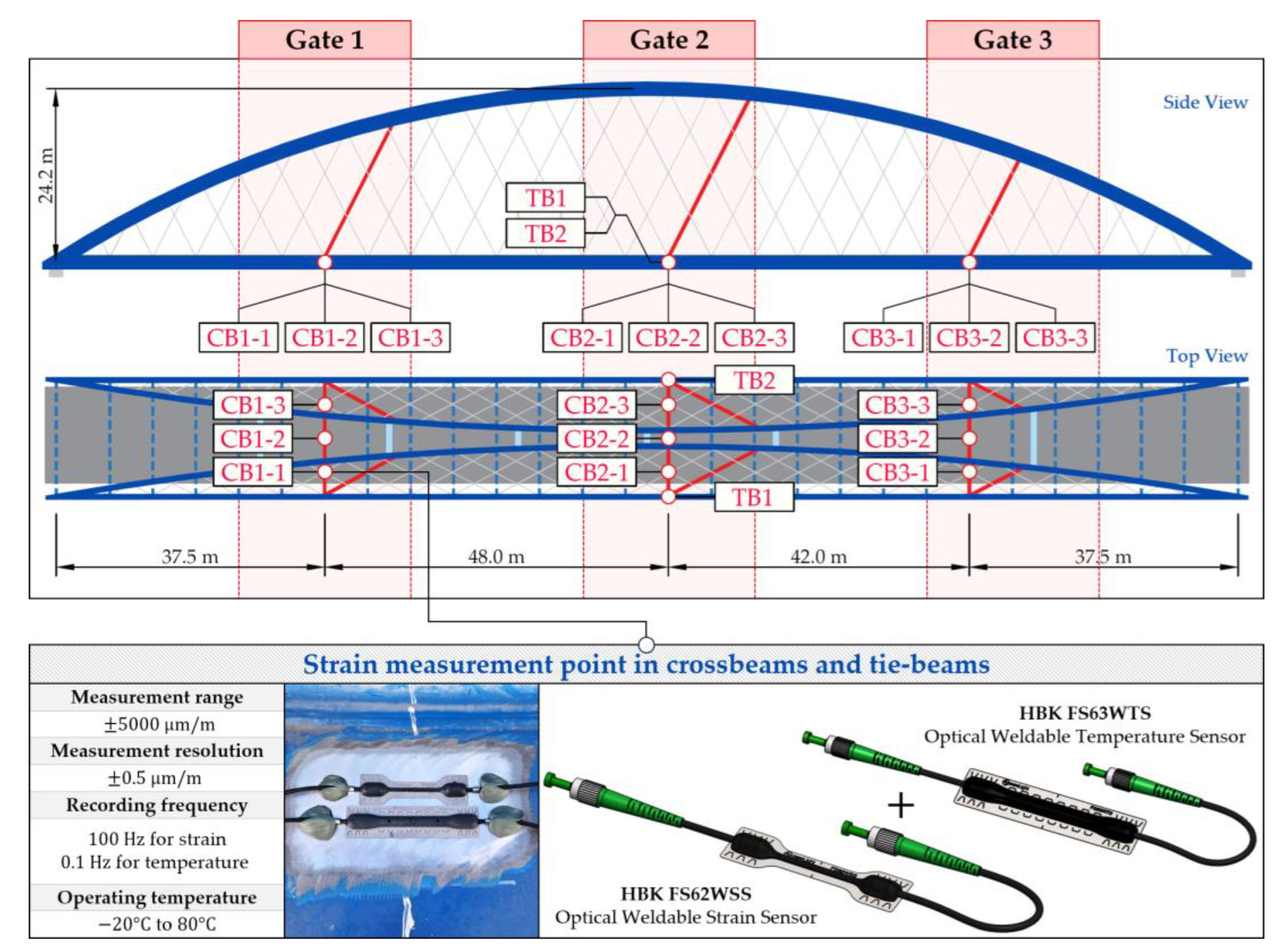
Figure 2.
The measurement gates, arrangement, and characteristics of the bolted FBG sensors in the hangers.
Figure 2.
The measurement gates, arrangement, and characteristics of the bolted FBG sensors in the hangers.
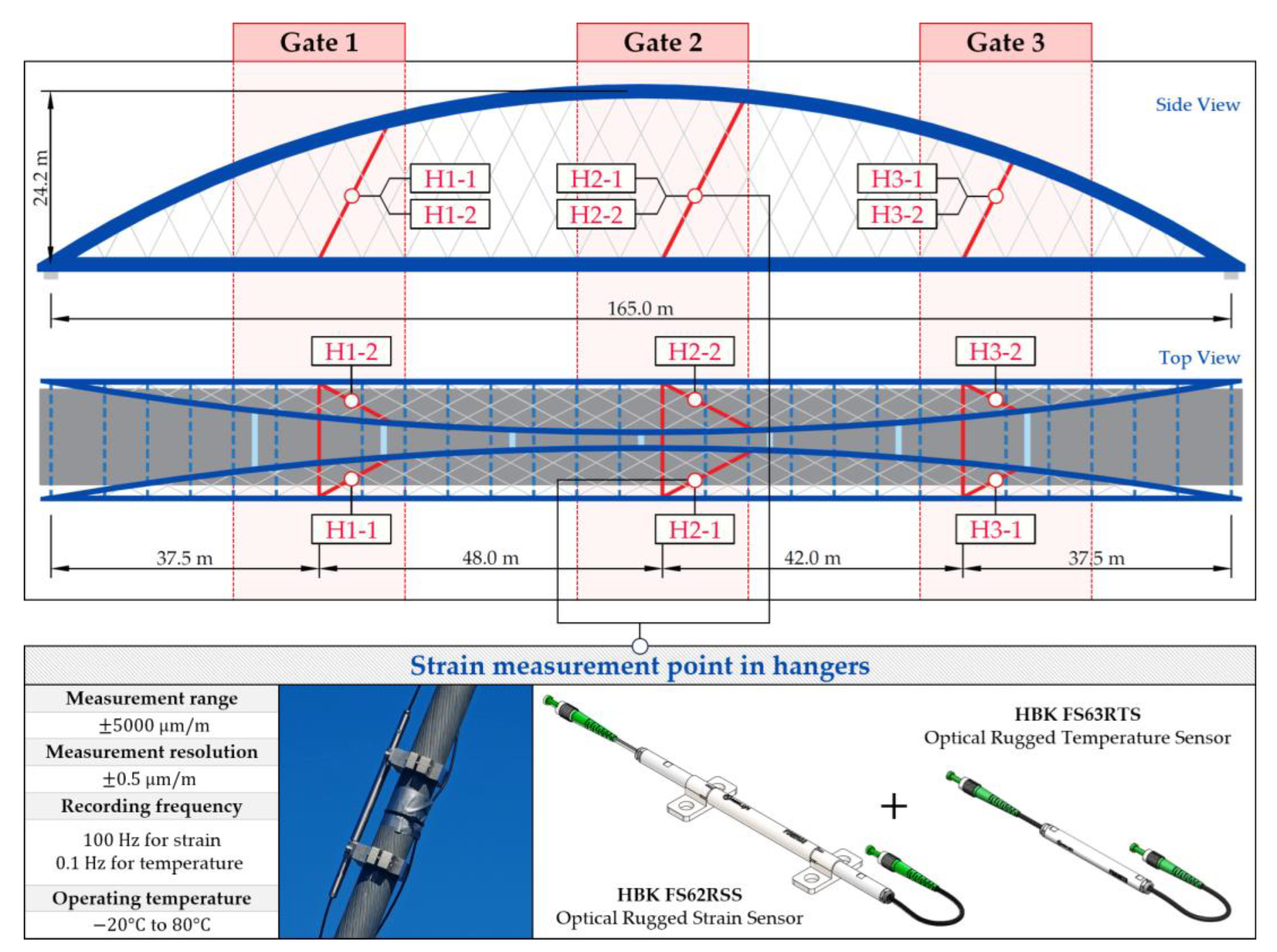
Figure 3.
Strains in the crossbeam at the gate no. 3 during dynamic load test passage.
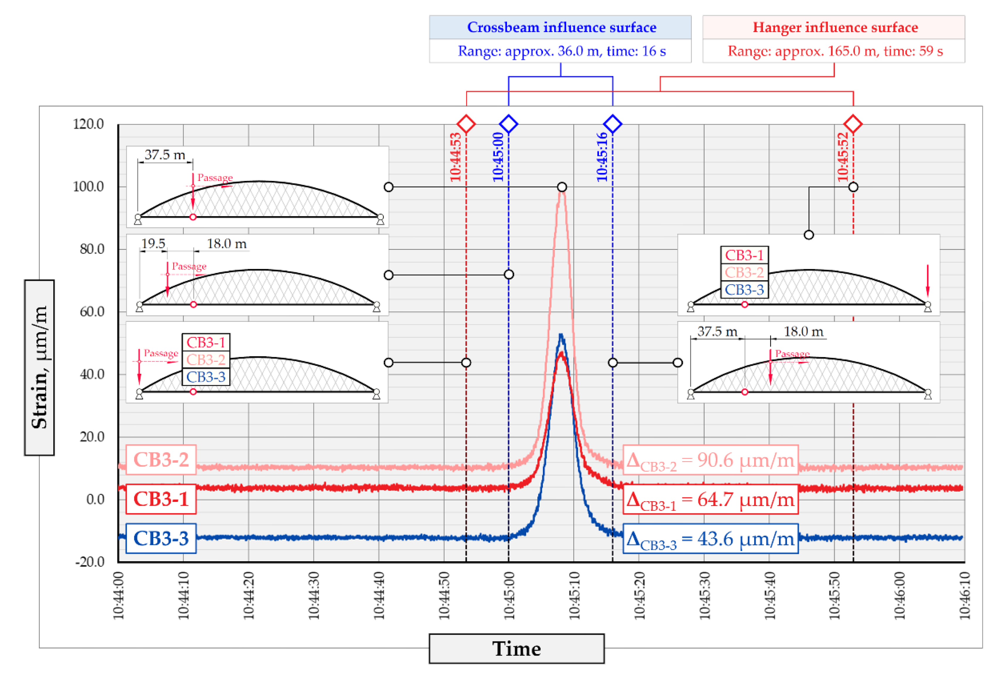
Figure 4.
Strains in the hangers at the gate no. 1 during dynamic load test passage.
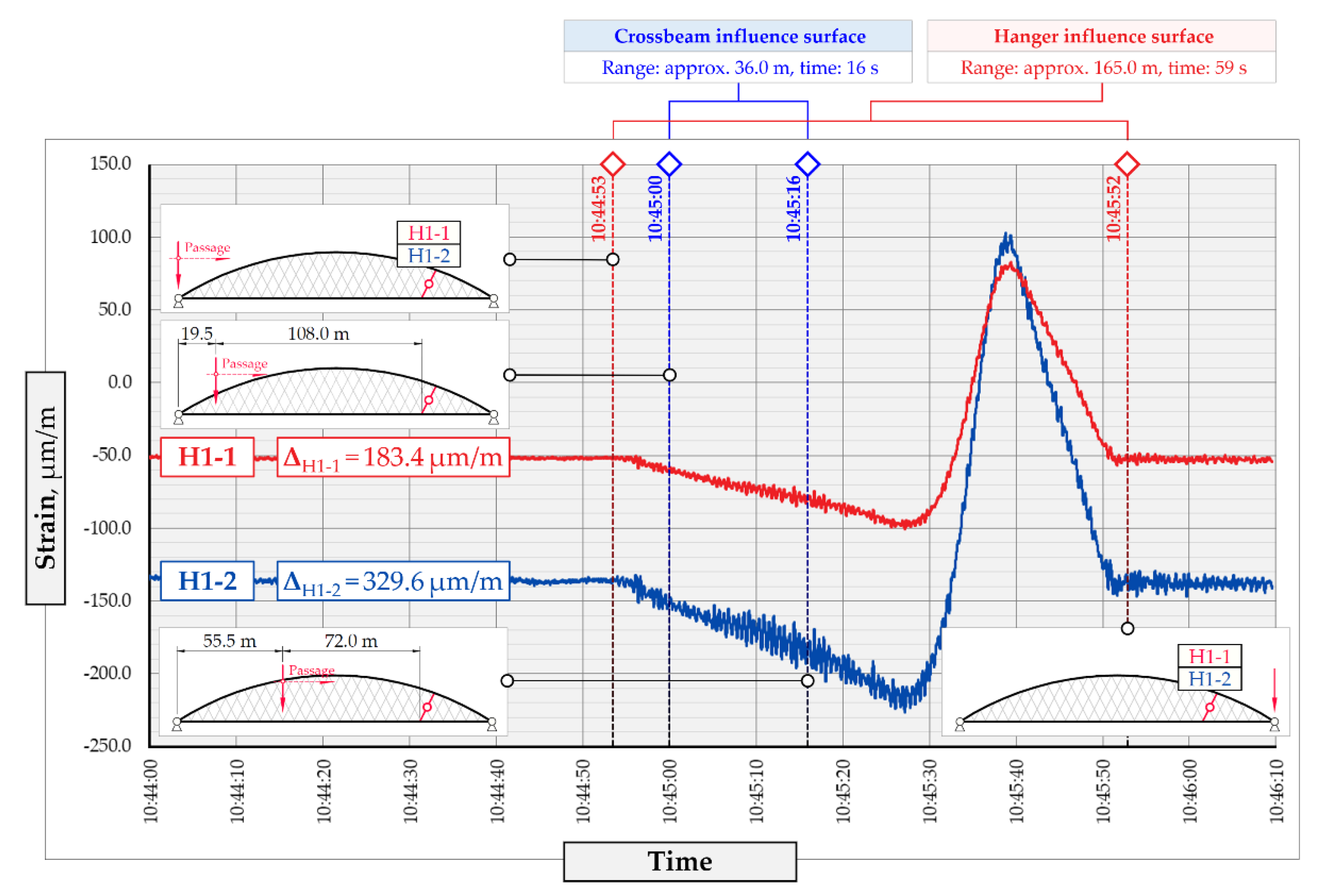
Figure 5.
SHM system framework.
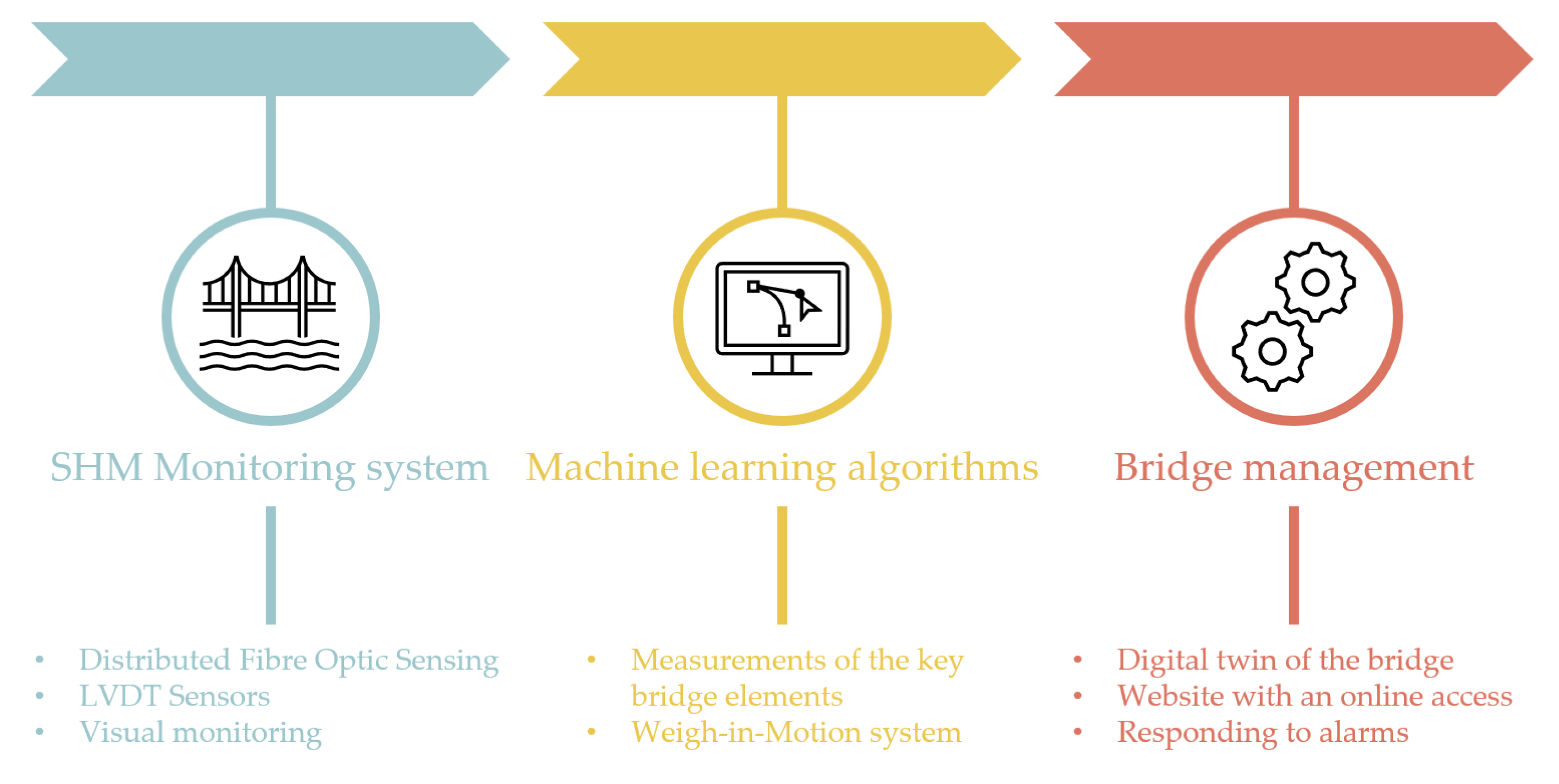
Figure 6.
The procedure of establishing the BWIM module, including the SHM system, load testing, FE model adjustment, and ML regression algorithms.
Figure 6.
The procedure of establishing the BWIM module, including the SHM system, load testing, FE model adjustment, and ML regression algorithms.
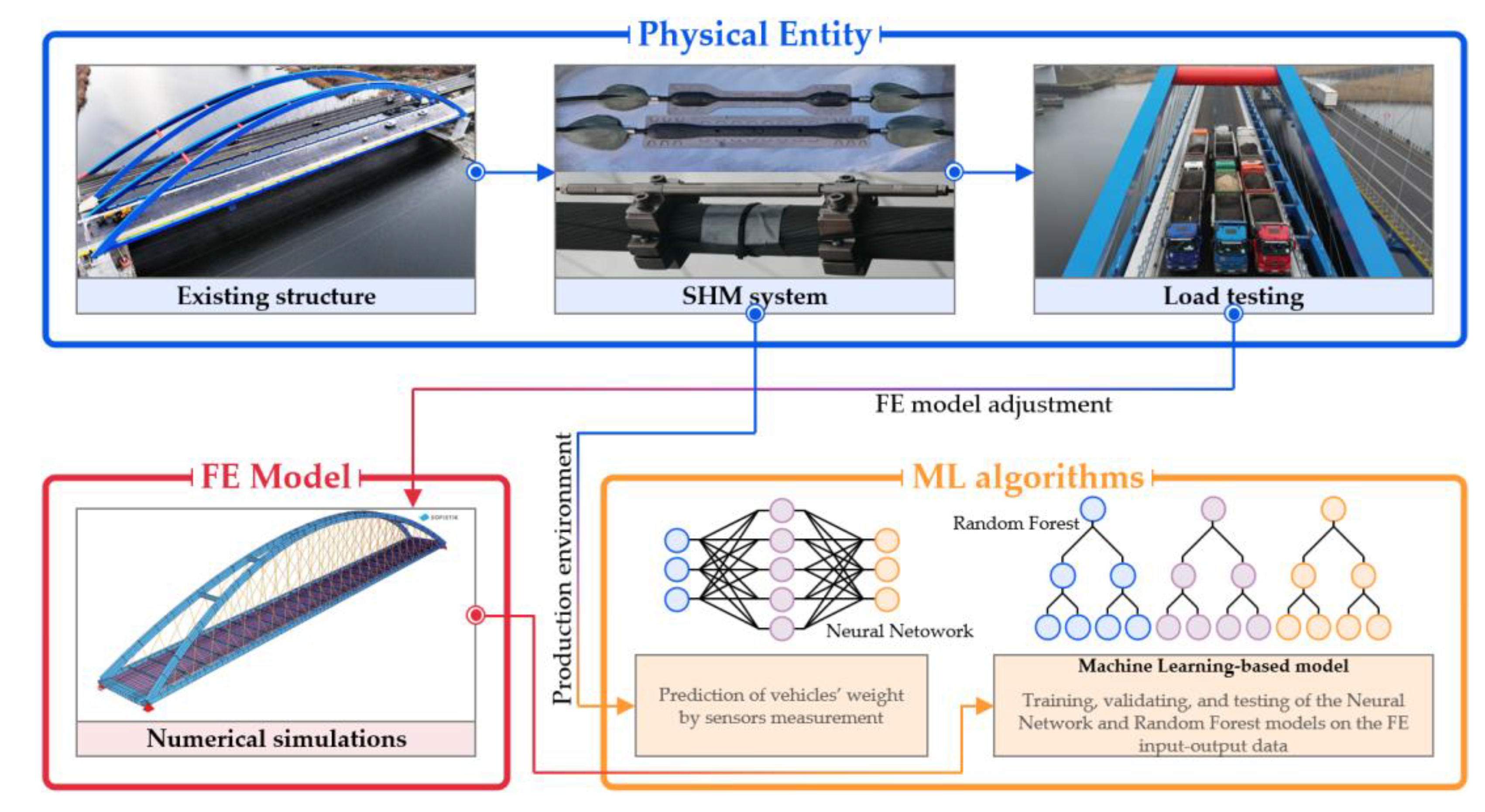
Figure 7.
The procedure of establishing the BWIM module, including the SHM system, load testing, FE model adjustment, and ML regression algorithms.
Figure 7.
The procedure of establishing the BWIM module, including the SHM system, load testing, FE model adjustment, and ML regression algorithms.
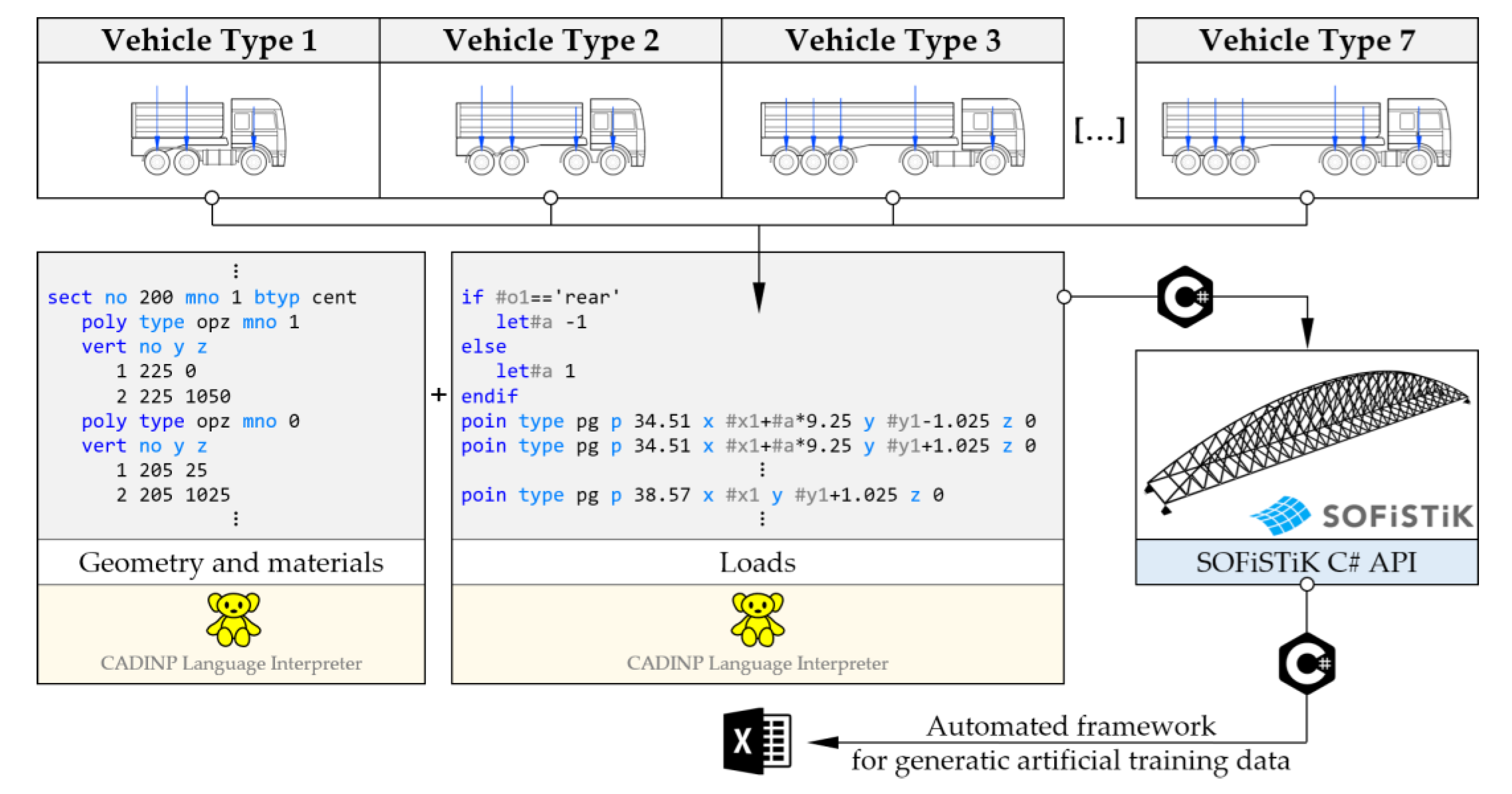
Figure 8.
Weight RMSE for different RF architectures with 17 inputs.
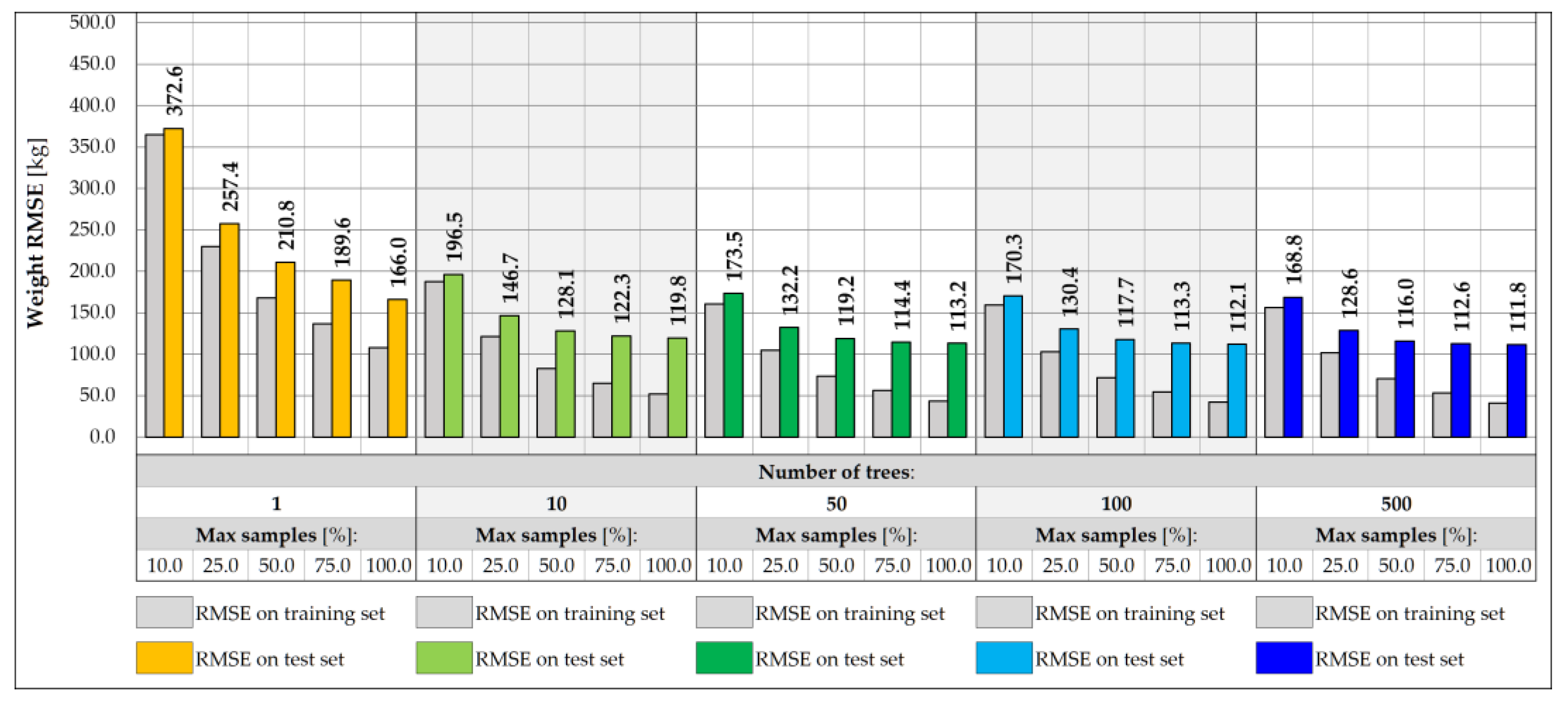
Figure 9.
Coordinate Y RMSE for different RF architectures with 17 inputs.
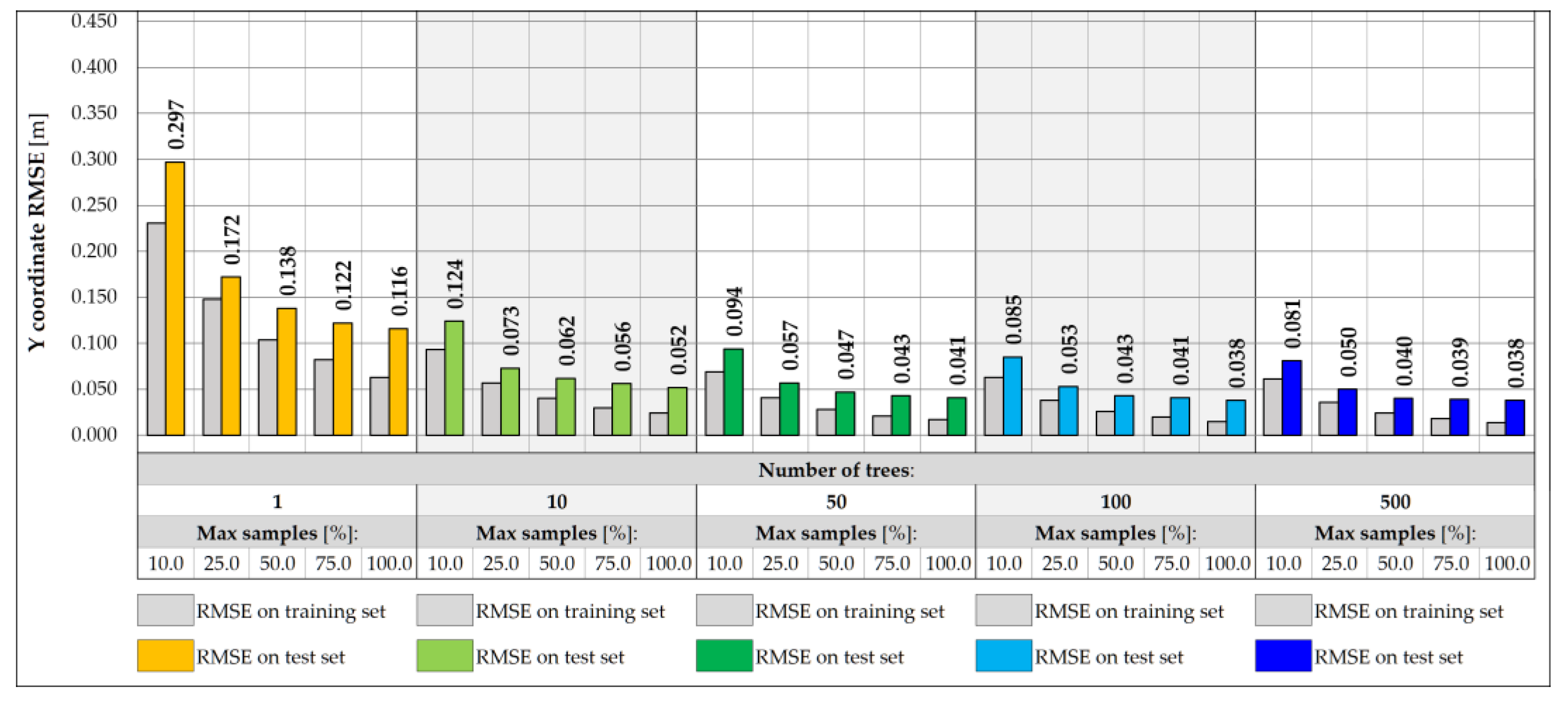
Figure 10.
Weight RMSE for different RF architectures with 5 inputs.
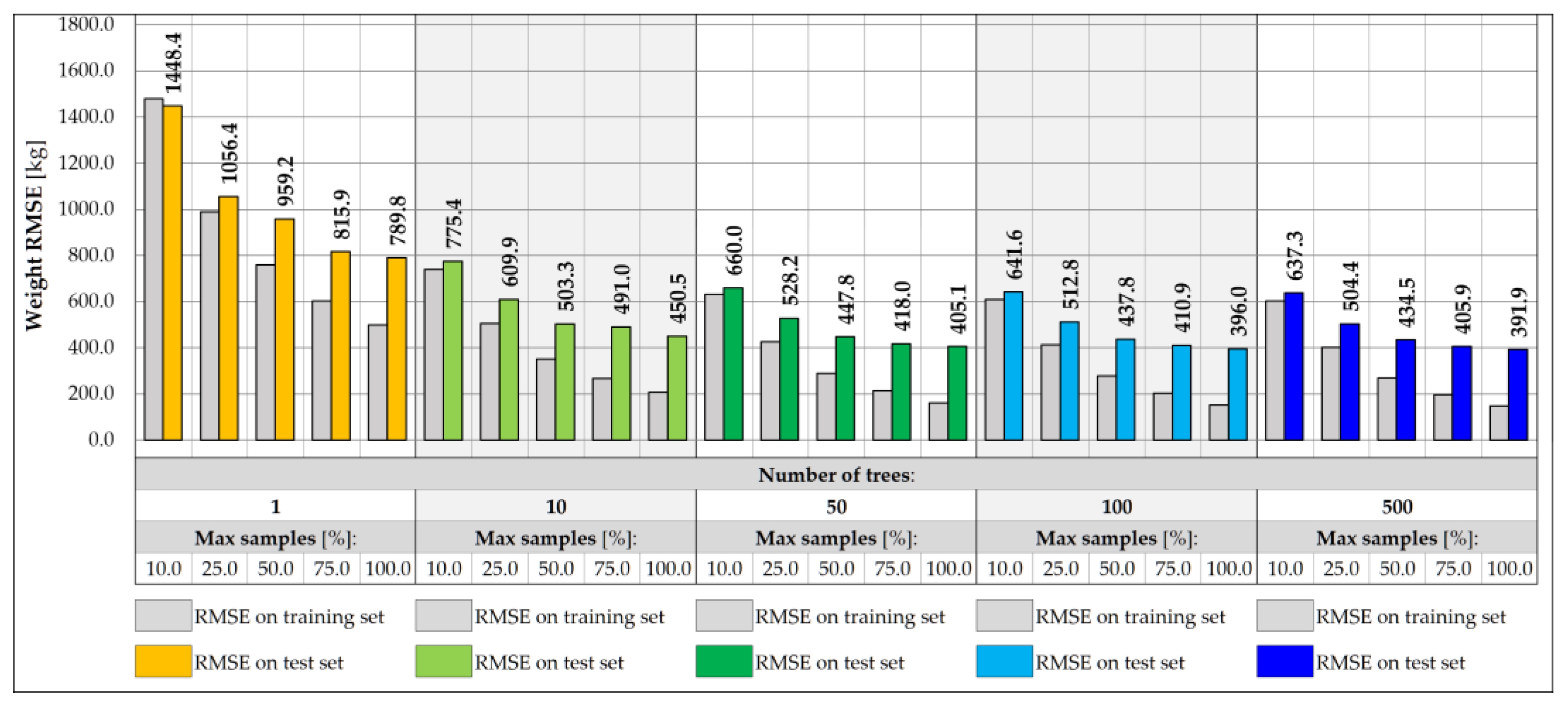
Figure 11.
Coordinate Y RMSE for different RF architectures with 5 inputs.
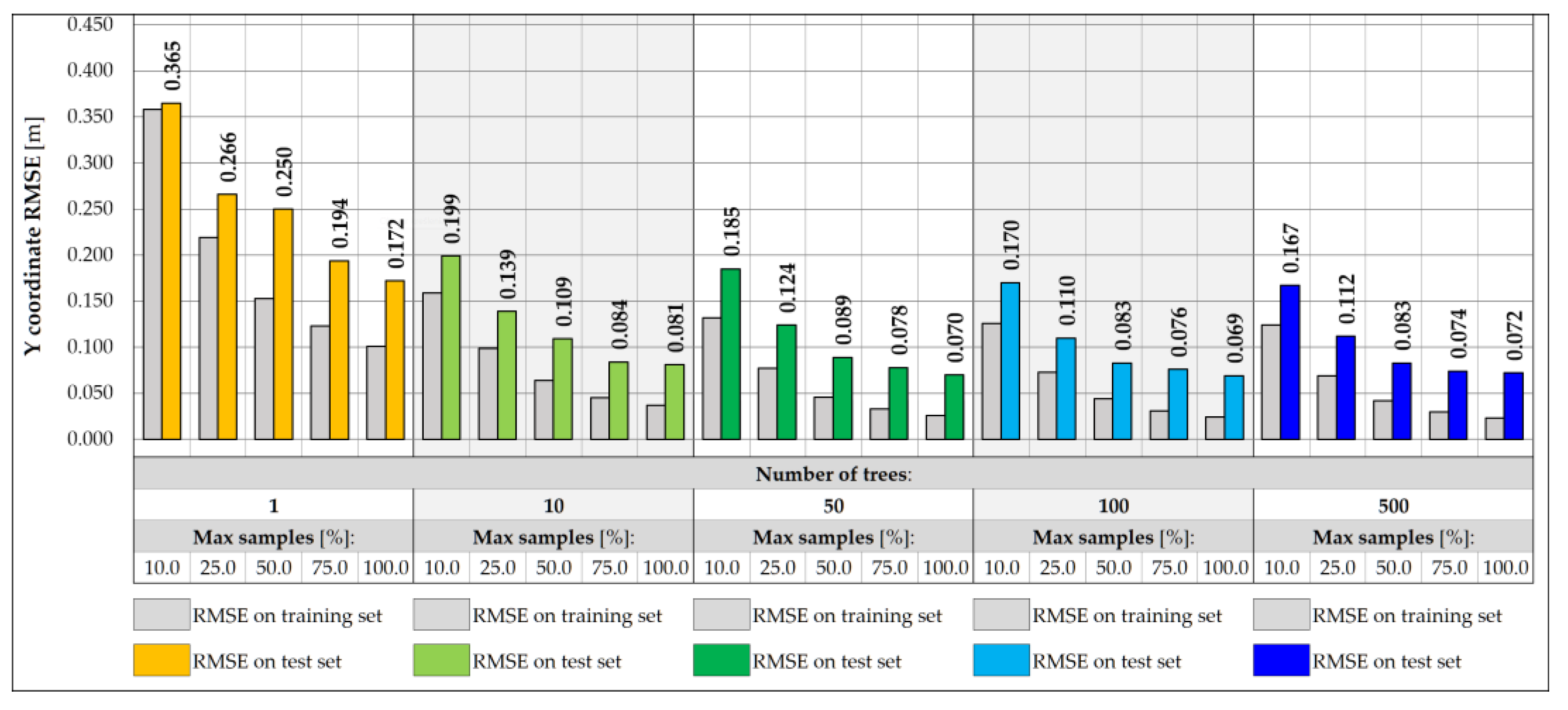
Figure 12.
Weight RMSE for different RF architectures with 3 inputs.
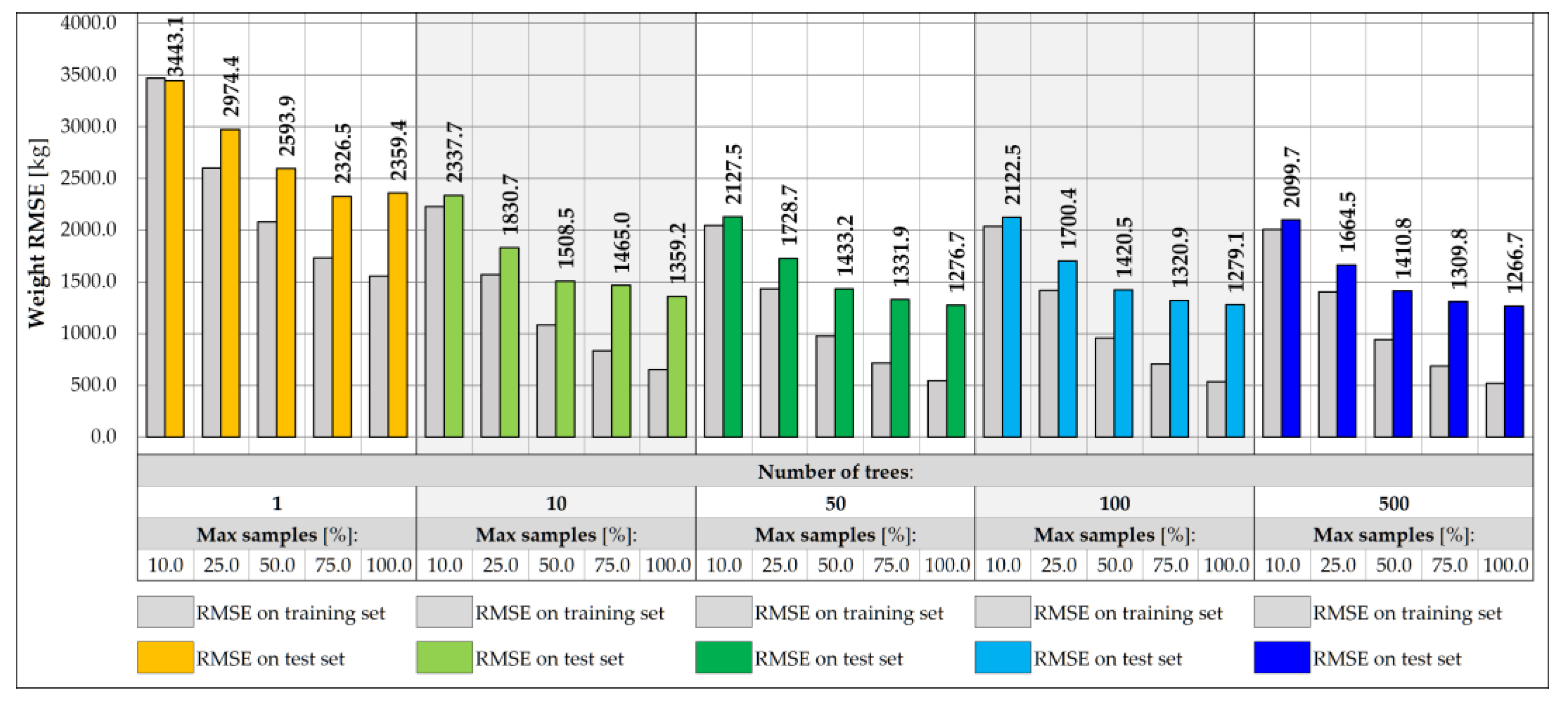
Figure 13.
Coordinate Y RMSE for different RF architectures with 3 inputs.
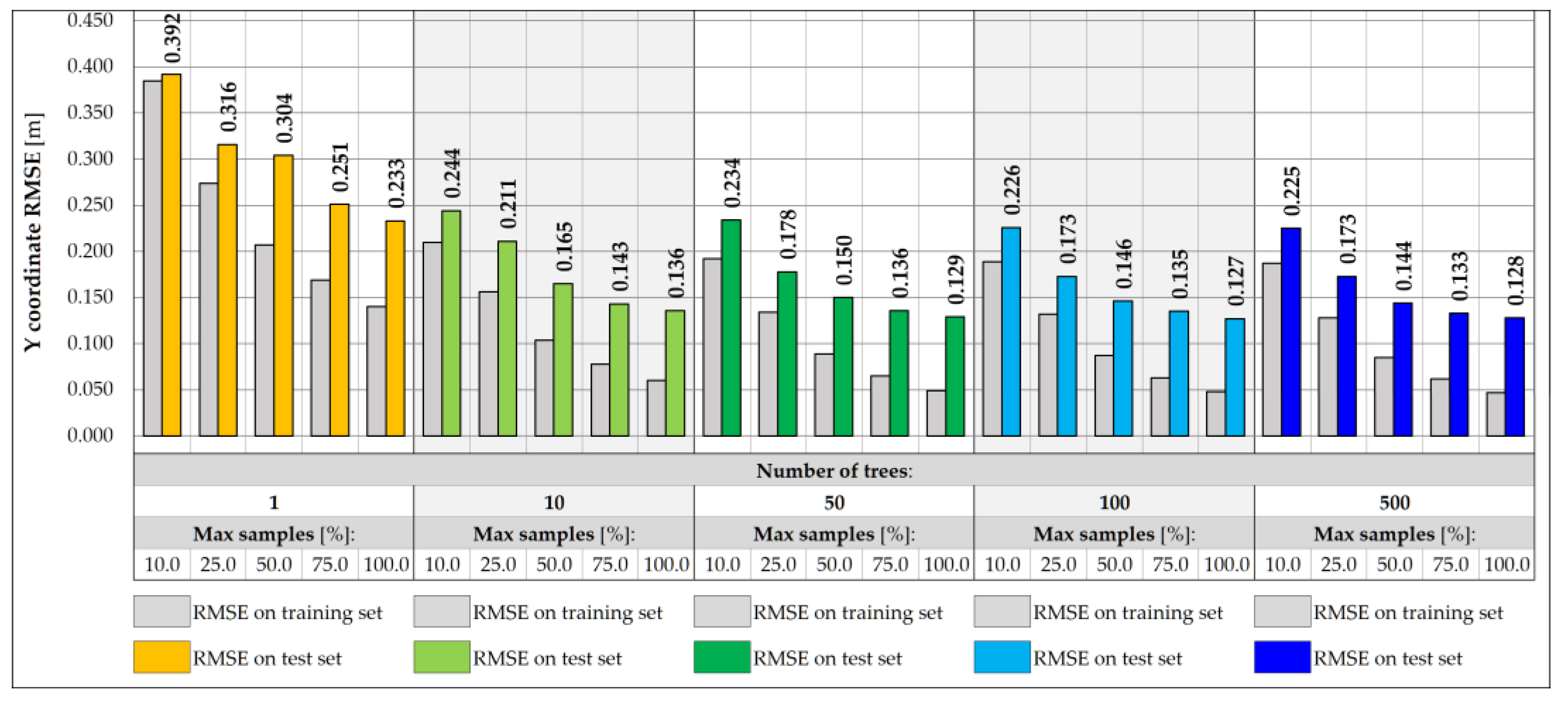
Figure 14.
Weight RMSE for different NN architectures with 17 inputs.
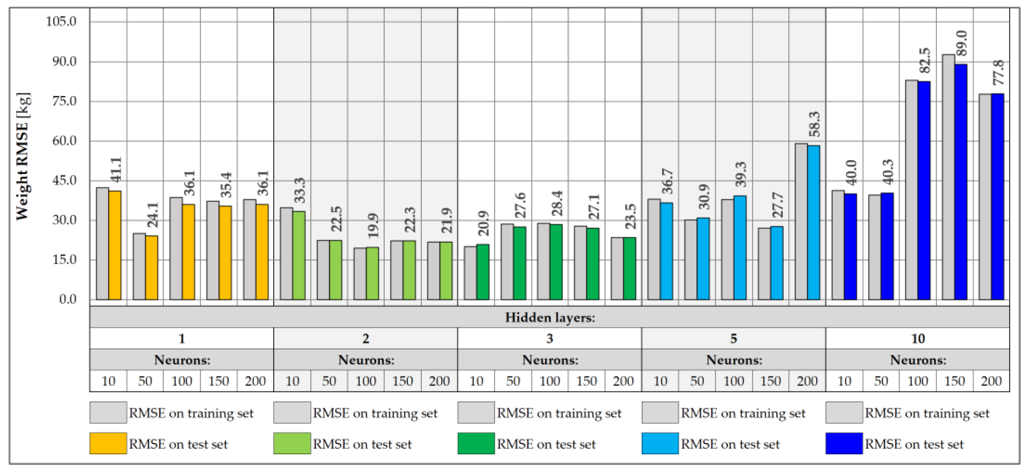
Figure 15.
Coordinate Y RMSE for different NN architectures with 17 inputs.
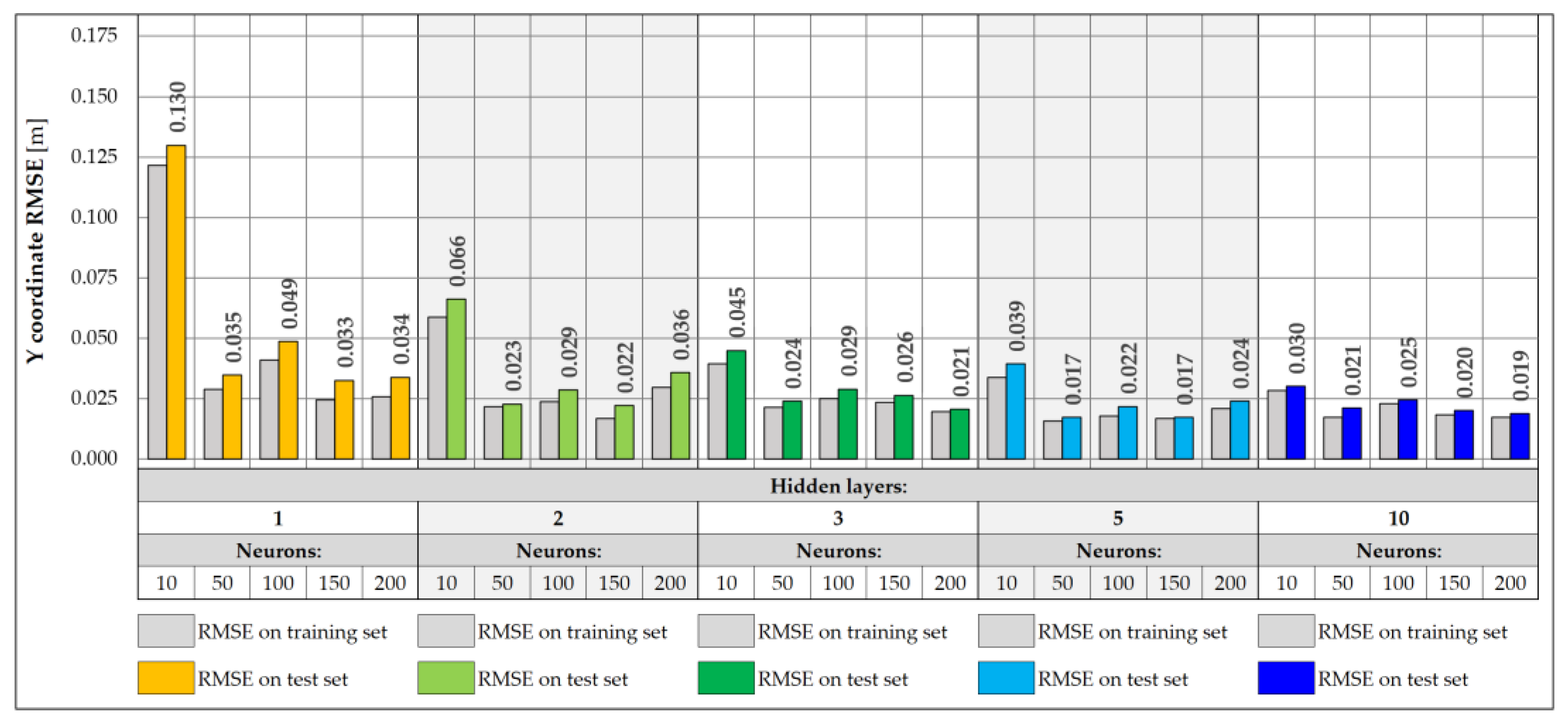
Figure 16.
Weight RMSE for different NN architectures with 5 inputs.
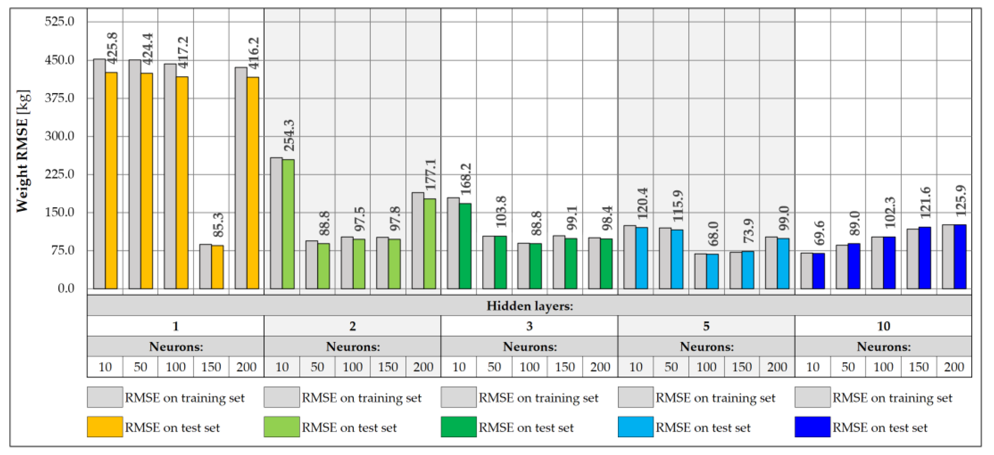
Figure 17.
Coordinate Y RMSE for different NN architectures with 5 inputs.
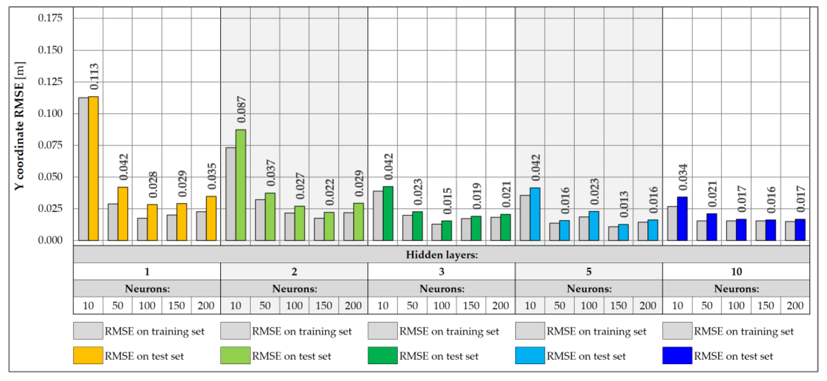
Figure 18.
Weight RMSE for different NN architectures with 3 inputs.
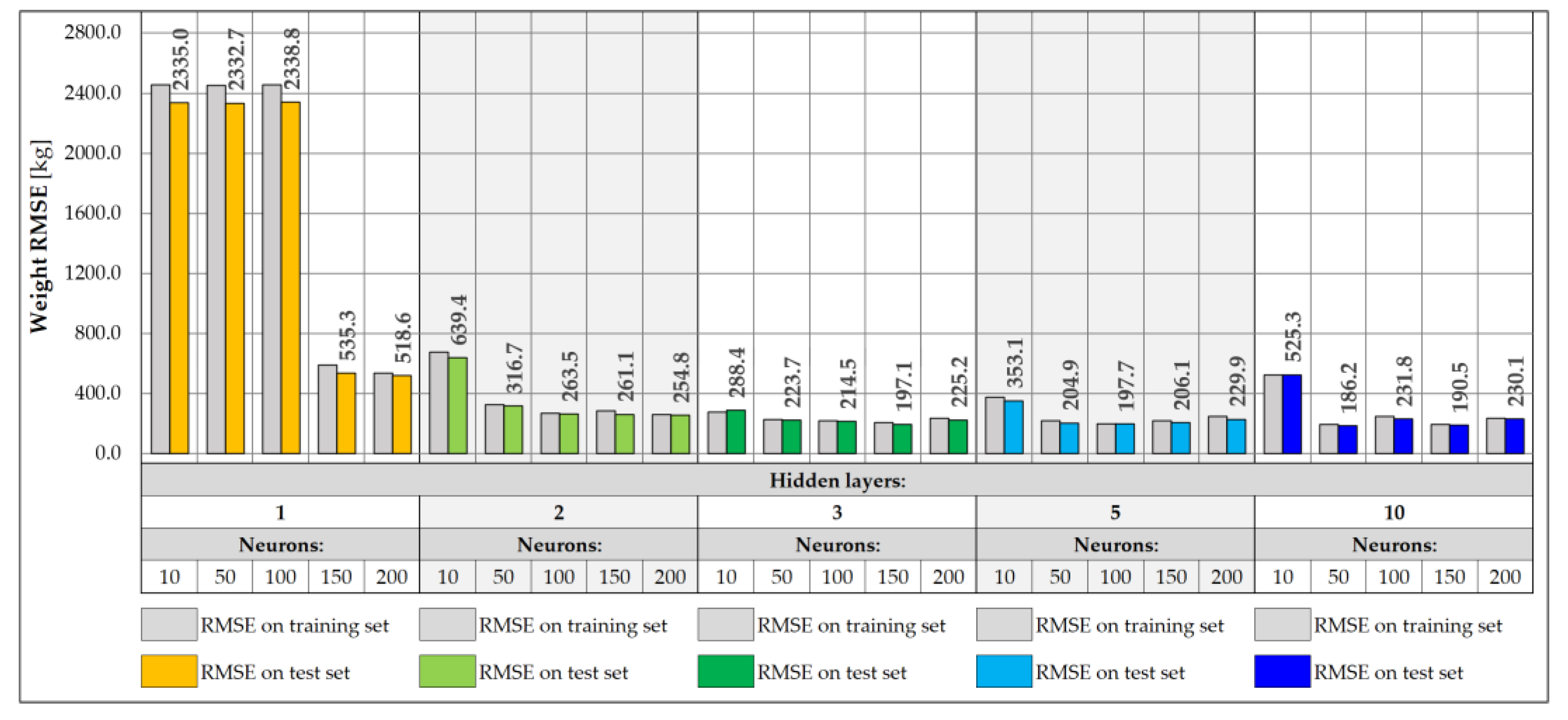
Figure 19.
Coordinate Y RMSE for different NN architectures with 3 inputs.
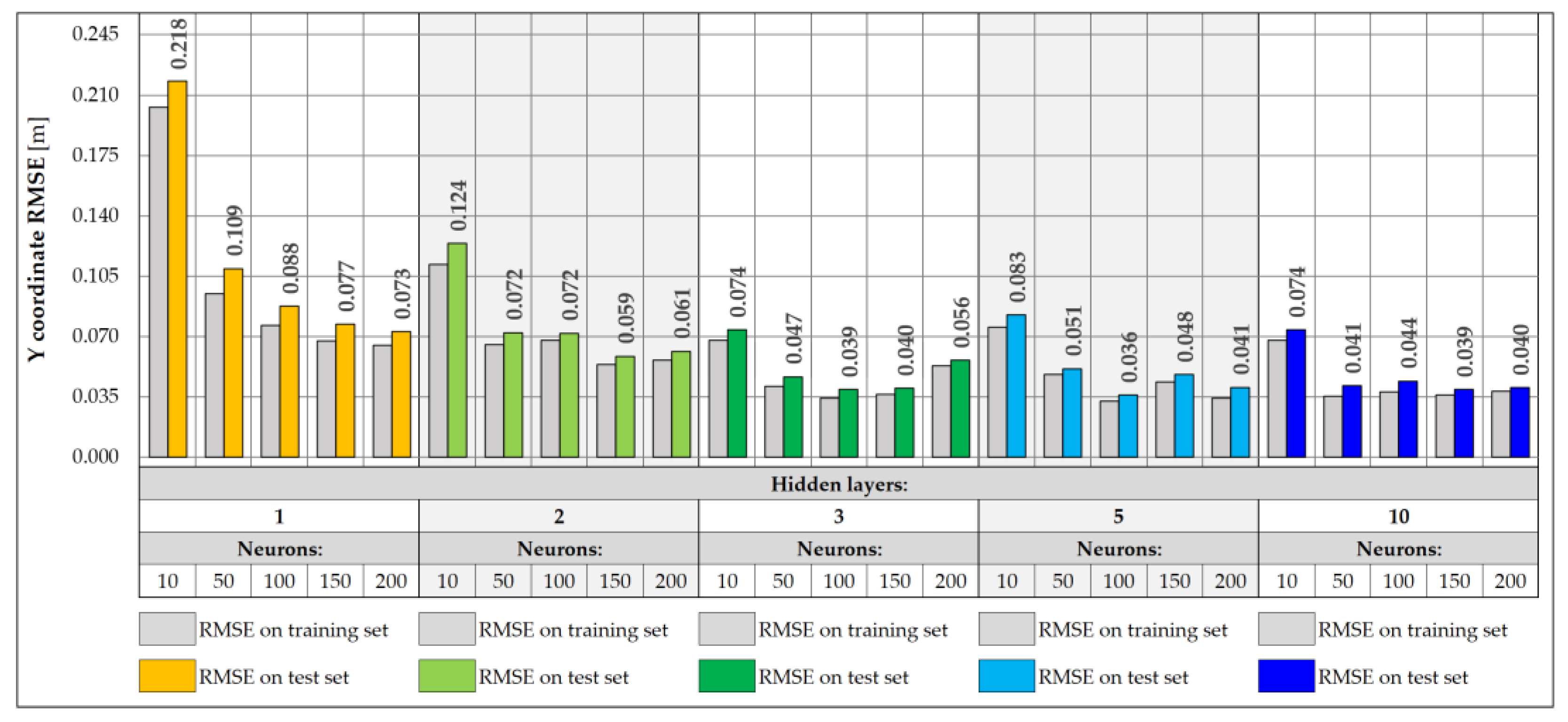
Figure 20.
Regression model for measurement uncertainties.
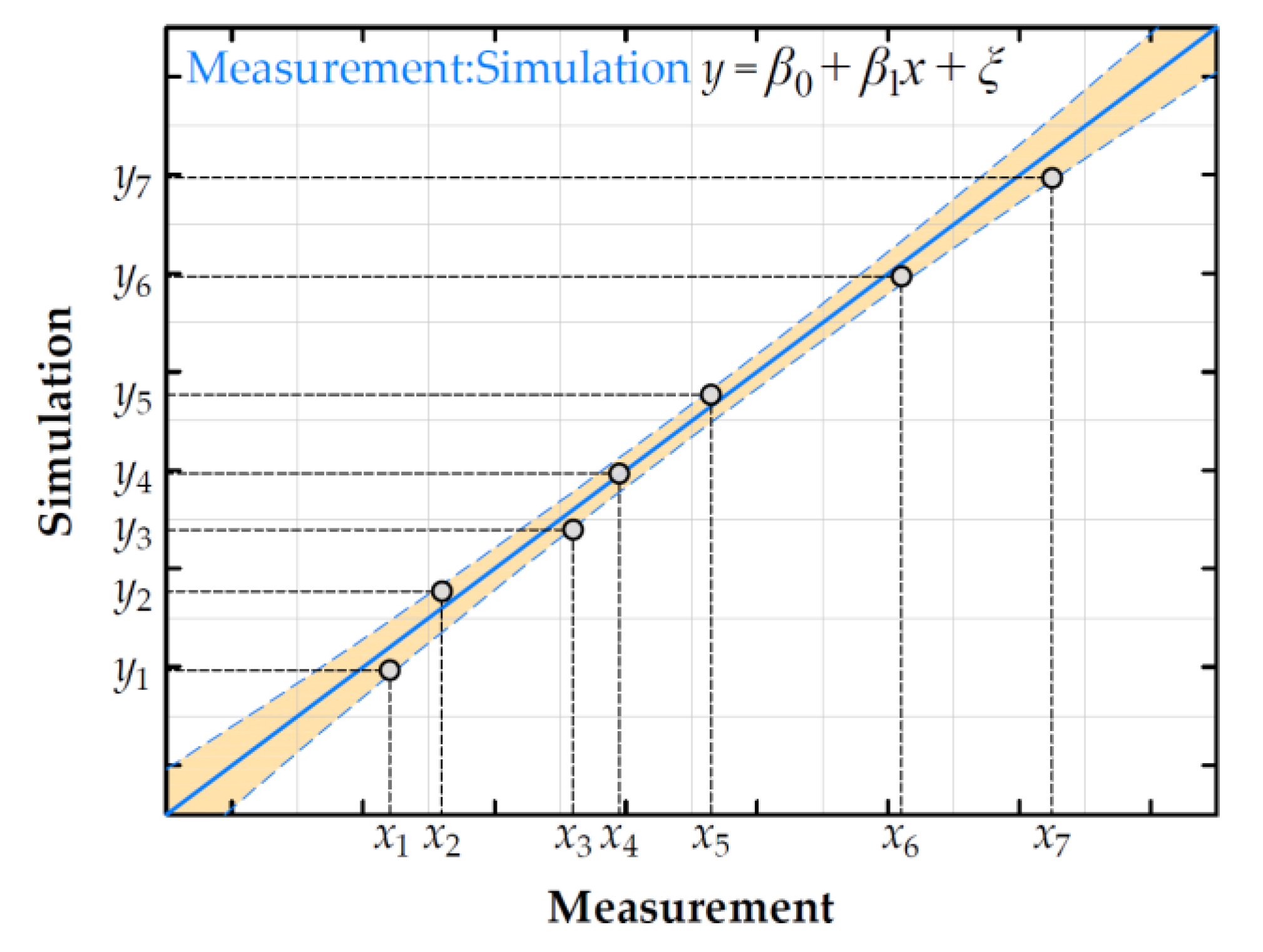
Figure 21.
Regression models predicting the weight of vehicle based on 3-input vector: a) Neural Network regression model, b) Random Forest regression model.
Figure 21.
Regression models predicting the weight of vehicle based on 3-input vector: a) Neural Network regression model, b) Random Forest regression model.
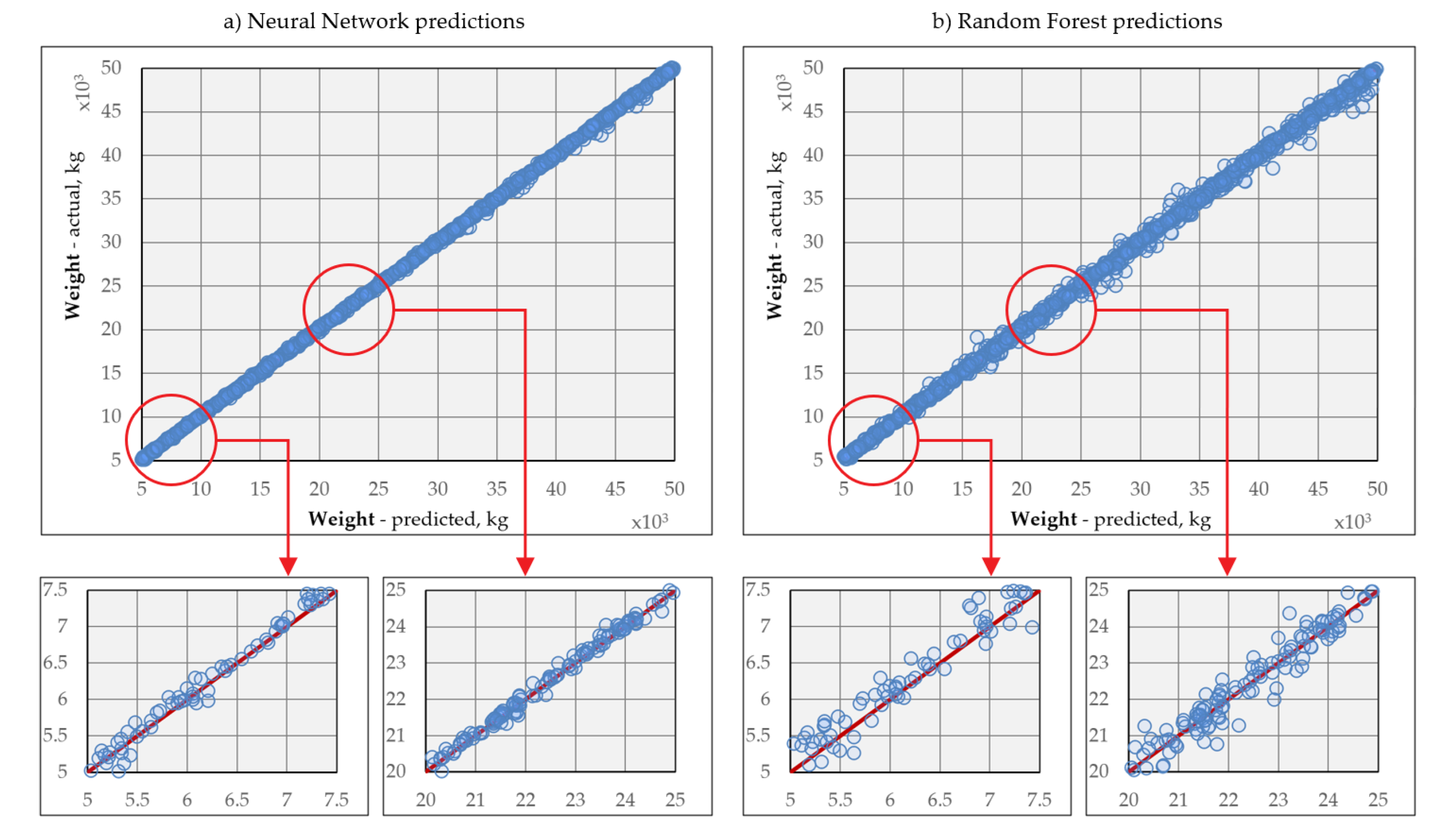

Table 1.
Comparison of accuracy and learning time for different sizes of training set.
|
Random Forest Regression: Total weight estimation number of trees: 500, max samples: 100.0% | |||
| Training set size | Training time 1 [s] | RMSE [kg] | |
| Training set | Test set | ||
| 4 800 | 5.5 | 518.1 | 1 266.7 |
| 12 000 | 14.4 | 356.8 | 883.4 |
| 24 000 | 33.1 | 271.9 | 674.1 |
| 48 000 | 73.2 | 197.7 | 509.6 |
1 Personal Computer, processor: Intel Core i9-14900HX, 32.0 GB RAM, GPU 12 GB.
Disclaimer/Publisher’s Note: The statements, opinions and data contained in all publications are solely those of the individual author(s) and contributor(s) and not of MDPI and/or the editor(s). MDPI and/or the editor(s) disclaim responsibility for any injury to people or property resulting from any ideas, methods, instructions or products referred to in the content. |
© 2025 by the authors. Licensee MDPI, Basel, Switzerland. This article is an open access article distributed under the terms and conditions of the Creative Commons Attribution (CC BY) license (http://creativecommons.org/licenses/by/4.0/).
Copyright: This open access article is published under a Creative Commons CC BY 4.0 license, which permit the free download, distribution, and reuse, provided that the author and preprint are cited in any reuse.


