
Submitted:
21 August 2025
Posted:
22 August 2025
You are already at the latest version
Abstract
An averaged soliton occurs when a soliton propagates through a medium that is periodically heterogeneous. The reason is that the propagation in a homogeneous medium is consistent with the stability consideration of a single eigenvalue spectrum, even in the cases of loss and amplification processes. This assumption changed in tandem media where we considered local changes. In this paper, we focus on the nonlinear dynamics and show that optical solitons, both temporal and spatial, reshape into a nonlinear modulation from medium to medium when they propagate through a periodically stratified nonlinear medium. It can be locally linearized as a perturbation near the corresponding soliton eigenvalue. We analytically and numerically discuss two particular optical soliton problems to show their generality: that of a Two-Level Atom medium (TLA) and a Kerr nonlinearity as a description of those materials and photorefractive materials. We can conclude that rather than a mean soliton, we have a modulated soliton.
Keywords:
photonics crystals
; photorefractive and Kerr materials
; resonant pulse propagation
; solitons
1. Introduction
Nonlinear pulse dynamics has proven itself as a significant area of physics, particularly in the optical regime, where it has found a sensible experimental test bed and practical applications, due to the ready availability of intense coherent light sources and nonlinear materials. The landmarks go from resonant pulse propagation, optical fibers, and self-guiding of light [1,2]. The first optical Solitons in Optics and Photonics were the resonant Temporal Solitons in Self self-induced transparency [3], and that became one of the mainstreams of physical optics. They introduced fundamental concepts such as the area theorem, which is a description of the convergence to the actual soliton eigenvalue, and a thorough analysis of the variety, behavior, and interaction of solitons. Complex coupled soliton systems were also introduced, such as the simultons [4], ancestors of the current quantum security. Since then, most of the attention has been focused on non-resonant solitons such as those produced by intensity nonlinearities. One of their most essential and visible applications, to the ordinary people, has been long-distance optical fiber communications. In these systems, interaction, loss, and periodic amplification of temporal solitons have been thoroughly studied and experimentally demonstrated [5]. A parallel development in spatial solitons has led to a new realm of optical information on self-guiding light, where the interaction between spatial solitons and more complex structures has garnered renewed attention [6,7,8,9,10,11], typically under the ideal conditions of a homogeneous, unlimited medium.
The amplification and loss of temporal solitons, and in general, intense pulse propagation, have received a great deal of attention, particularly for optical communication applications. There, the recovery of the original signal is a priority. To obtain the initial pulse, we can consider that the amplification process is adiabatic [12]. Pulse reshaping, then, is a purely internal nonlinear process that arises from the convergence of the pulse to specific eigenvalues of the nonlinear equation, reaching it as a steady state, characteristic of a given medium. However, the soliton consideration is at a long-distance limit. Therefore, the actual reshaping process has received limited attention. Thus, a periodic array of nonlinear media may freeze such transient behavior into a periodic one. There is an increasing interest in the study of propagation through heterogeneous media, in particular, in periodic arrays or Tandems of media sections larger than the wavelength, or Bragg reflectors [13,14]. On the one hand, this sets the problem beyond the scope of photonic crystals and their coherent reflection and transmission process; therefore, we limit ourselves to the transmission. These periodic heterogeneous systems have garnered significant attention in Nonlinear optics due to their consideration of tandems of quadratic nonlinearities and linear media sections [15], resonant [16,17], including split-step fiber links where Kerr nonlinearities alternate with linear segments [18]. Some other works included fully nonlinear tandems around a mean value [19] or in the extreme of opposite signs [20,21]. In these tandems, we can find focusing and defocusing effects, a different profile for each nonlinearity [22], or study the solitons as a result of a coupled NLSE [23]. Even when these works refer to a pulsating soliton [24], they do not refer to the essential process of reshaping, other than the tandem modulation. There are also some reviews on the general aspects of this topic [25,26,27,28], and there is a promising experimental potential that still has to be explored more thoroughly [29].
We will describe our tandem as a structure with a period , where and are the lengths of each medium are both much larger than a wavelength. Therefore, we disregard the reflected signal. The interaction of a soliton with interfaces has been analyzed [30]; however, the propagation of solitons in different media is becoming increasingly important.
We show in the second section of this work that optical solitons propagate through a nonlinear, periodically stratified medium, where reshaping from medium to medium results in a nonlinear modulation. We also show that it can be locally linearized as a perturbation near a soliton and analytically studied in a two-level atom (TLA) medium. The area theorem is also a straightforward description of the evolution of the resonant eigenvalue, even in the case of more than one medium, and therefore will be the guiding topic of this section. Our idea is to lay the groundwork for understanding more complex, intensity-dependent cases. The third section uses the previous results to describe the soliton continuous reshaping process that occurs in Kerr and photorefractive materials. The pulse amplitude is related to the Kerr eigenvalue, although we do not have an additional description such as the area theorem. Therefore, we should present our findings graphically, and we based our discussion on our results in the resonant case. The reader will corroborate that these graphs are essential to understanding this case. Finally, in the fourth section, we present our conclusions.
2. Resonant Pulse Analysis
The Maxwell-Bloch Equations describe the lossless propagation of near-resonant light pulse propagation in a Two-Level Atoms (TLA) atomic medium, given by:
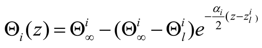
where and are the in and out of quadrature dipole terms, is the atomic inversion. Δ is the atomic detuning, Ω = 2dE is the Rabi Frequency. Θ usually express the area of the pulse, but in fact, it corresponds to the area of the Rabi frequency area, and in this work, this will be a substantial difference.
there is the actual area of the pulse, which satisfies the equation:
where both and the absorption coefficient α depend on the material. The well-known area theorem describes the solution of Equation (5) depicted in Figure 1 as a function of z and Θ for that material.
The soliton spectrum behaves as a collection of equally spaced attractors surrounded by their basins of attraction, without any overlap, which also corresponds to the corresponding branches of the area theorem. The propagation of two Different TLA materials, A and B, is shown pictorially in Figure 1b. While their spectra are the same, they are not identical. Their scaling is different because of the different dipole constant; however, they still will correspond to 0π, 2π, 4π, … attractors. The pulse-reshaping that occurs in material A depends on its initial value. This fact restricts its evolution to an attractor or branch in the area diagram. The evolution through a distance (thick arrow in A) results in a value Θ when it is interrupted by the change of materials, and then it turns into a new initial value for the material B (broken arrow). There, the new material coefficients produce a new reshaping process through a distance , starting all over again. The continuous process, back and forth between the two spectra, corresponds to a periodic propagation in two different TLA materials, and corresponds to the solution of the equations:
In the period. If both areas’ initial values are such that , << π, then both can be linearized and both will satisfy Beers law and , where . This decay discontinuity produces a stepwise exponential decay that converges to the single identical attractor 0π.
In the case of propagation near a higher-order attractor, we can linearize these equations, which represents an attractive problem of perturbation near a soliton eigenvalue. Then it is simplified by the description of the eigenvalue provided by Equations (7) and (8). We can rewrite the soliton solution for the media in the slab as
The solution for Equation (9) is given by:
where we can quickly recognize that the sign of the term corresponds, in the positive case, to the convergence of the steady state from below in the graphical representation of the area theorem. In the negative case, to an analog of the decay of the Beers law. If the description considers the terms of the pulse area that is continuous between the different media, for a specific period, we can rewrite it as:
The solution in the first medium, where and . is the initial value in the period and is the previous distance in number of periods. In the second medium , the corresponding expression is given by:
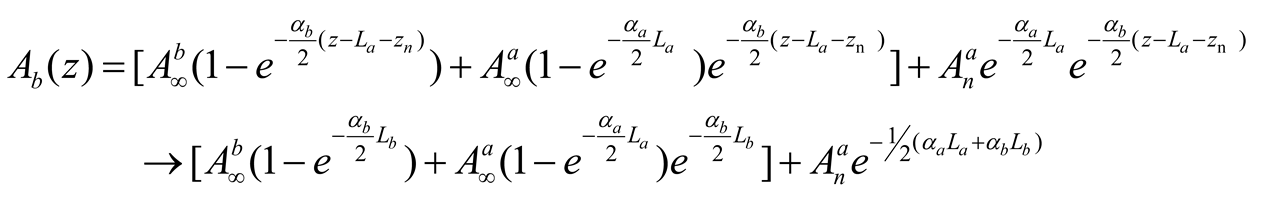
In the second line, we have written the expression at the end of that period. Suppose we consider long material conditions; i.e., y , we are describing a sequence that selectively oscillates, without mixing the information of the two solitons, and its behavior will be strictly periodic, as depicted in Figure 2.
At the end of each period, the area will reach a value of . However, if one medium is small, the enunciated conditions are not satisfied for that medium, although they are satisfied by the other one, which will lead to a periodic behavior, as can be seen in Figure 3 and Figure 4.
If and
If and
Finally, if both media are small, i.e., if and then, there is a clear memory of the initial conditions in the period, losing the periodicity, Figure 5,
We take Equation (15) to perform numerical simulations, setting the following: values, . We also want to remark that we changed only the width of the slab. The input area has been set to six rad for all sequences.
We explored the oscillation near the same soliton eigenvalues, and we can rely on the stability of the propagation. However, there are a large number of possibilities where these conditions will not be satisfied and where we will need to consider in detail the resonant solitons behavior. For example, the case of 4π solitons tends to break into two 2π solitons, and those are somewhat sturdy, as well as there is a rich collection of 0π pulses, whose coupling will add additional features worth exploring by the adequate atomic systems. That may include the current interest in V and Λ atomic systems. We can find different works showing the behavior of the pulse itself, such as amplitude, width, and energy.
3. Photorefractive-Kerr Analysis
In this section, we numerically study the behavior of a soliton subject to a periodic sudden profile reshaping due to the change of the propagation material. The nonlinear materials involved here were photorefractive and Kerr nonlinearity type, where we had studied the photorefractive-photorefractive, photorefractive-Kerr, and Kerr-Kerr cases. The evolution into the corresponding soliton is a possibility if we provide a sufficient distance in each region. However, the Kerr soliton is much more complicated. The interference of the reshaping with this behavior leads to a much more complex dynamics, and we present here only the results for the case of Kerr-Kerr periodic media.
Because of space, we will assume that the two media have the same dimension, i.e., and . The sudden changes of material correspond to a step-like distribution of the Kerr constant. The equation we must solve for each material is the well-known Nonlinear Schrödinger Equation, given by:
where represents the original width of the beam and, is the initial amplitude of the complex envelope of the field. We normalize the propagation variable Z regarding the diffraction length, by and assigned the normalized transverse variable, and X, regarding the initial beam width, , by , the field amplitude was also normalized in terms of the initial field amplitude , using diffraction lengths as . Furthermore, we can write the nonlinear length as a function of initial field intensity and the nonlinear refraction index for “ith” media; then this length takes the form , where finally the nonlinear constant for the i-media is given by , where .
The solution of Equations (16) and (17) are well-known solitons, shown in Figure 6a, where the central peak amplitude provides the Soliton eigenvalue of the NLS. Therefore, in the absence of an equivalent to the area theorem of resonant pulse propagation, the convergence of the eigenvalues could be described by the central peak amplitude evolution, and we rely on numerical simulations. The peak amplitude exhibits a slight but perceptible fluctuation, as illustrated in Figure 6b, whose Fourier transform reveals that it is a cosenoidal modulation with a period dependent on the Kerr nonlinearity. We can characterize the peak by a relation of the form:
where the Fourier transform of is
and this spatial characteristic length is central to our description.
Figure 6b shows the linear frequency dependence on the nonlinearity, where the higher-order modulation is quite faint. Figure 7 illustrates the consideration of two different nonlinear media, showing an increase in fluctuations as the difference in nonlinearities increases.
Suppose the material period is smaller than . In that case, its changes will superimpose on this modulation, Figure 8. But if the frequency is of similar dimension, then it would modulate the fluctuations, Figure 9. From Figure 6b, we can notice that in our simulation, the period of the variation is in the range of , that will prove a critical relative parameter to define those domains.
If the length of the media is small, i.e., in the range of an , the frequencies of the changes due to the lengths of the media and those of the fluctuations are entirely different. We can see them as their superposition on the fluctuations, Figure 8. It is clear that the reshaping introduced by the change of materials is just a perturbation on the regular soliton oscillation and share features with the corresponding resonant case that we have already studied in the resonant case.
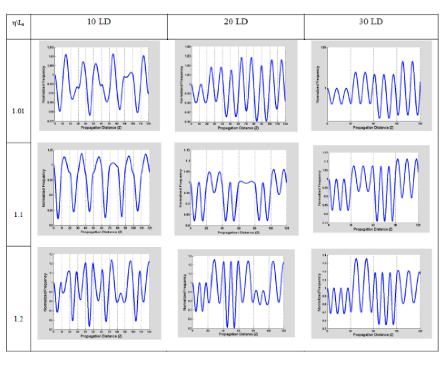
On the other hand, if the length of the media is in the range of the fluctuation’s characteristics length , i.e., larger than , then both frequencies are similar. The modulation is related with their superposition, as is depicted in Figure 9. However, we can not consider it as a perturbation anymore, but apparently as a distinguishable modulation as shown in the last column, where we recover the original oscillations of the corresponding soliton, Figure 6 with an envelope produced by the media, resembling the long-distance result in the resonant case.
4. Conclusions
We have discussed the temporal and spatial propagation of Optical solitons through a nonlinear material Tandem from a different perspective. We have focused our attention on the reshaping transients of two particular nonlinear systems, that of a resonant TLA medium and a Kerr medium. We have demonstrated that, depending on the dimensions of the Tandem sections, we can freeze the transient features of the reshaping in a Tandem process. Where the reshaping from media to media results in a nonlinear modulation, which can be locally linearized as a perturbation near a soliton and analytically studied in a TLA medium. This claim sets the basis for the understanding of the much more complicated intensity-dependent cases, where such a handy description of the evolution of the soliton eigenvalue is not available. This nonlinear modulation overlaps with the natural nonlinear modulation and depends on the interplay between the dimensions of the media and the lengths of the nonlinear processes.
The detailed analysis of the pulse itself, governed by this behavior of the corresponding eigenvalue variable, still offers a vast number of opportunities. In particular, we will find elsewhere the consideration of nonlinearities of different characteristics, such as the quadratic and the intensity-dependent, such as those that describe Kerr and photorefractive materials, quite crucial for self-guiding of light. On its own, this soliton continuous reshaping process raises exciting questions. Indeed, the practical experience of resonant pulse propagation has not required such a detailed analysis as extensively as intensity-dependent nonlinearities. That calls for a comprehensive analysis of the pulse propagation to find out stable solutions and a transient solution made stable by the stratified medium.
Funding
SECIHTI and Universidad Michoacana de San Nicolás de Hidalgo partially fund this research through grants CBF-2025-G-1268 and CIC2025-19648, respectively.
Acknowledgments
The authors acknowledge professors Ljubomir Matulic and G. E. Torres-Cisneros for their work introducing optical solitons in México [31].
References
- Hasegawa, A.; Tappert, F. Transmission of stationary nonlinear optical pulses in dispersive dielectric fibers. II. Normal dispersion. Appl. Phys. Lett. 1973, 23, 171–172. [Google Scholar] [CrossRef]
- Hasegawa, A.; Tappert, F. Transmission of stationary nonlinear optical pulses in dispersive dielectric fibers. I. Anomalous dispersion. Appl. Phys. Lett. 1973, 23, 142–144. [Google Scholar] [CrossRef]
- Allen, L. (Leslie); Eberly J. H. Optical resonance and two-level atoms, 1st Ed.; Dover, 1987.
- Werner M., J.; Drummond P., D. Simulton solutions for the parametric amplifier. J. Opt. Soc. Am. B. 1993, 10, 2390. [Google Scholar] [CrossRef]
- Mollenauer L., F.; Stolen, R. H.; Gordon J., P. Experimental Observation of Picosecond Pulse Narrowing and Solitons in Optical Fibers. Phys. Rev. Lett. 1980, 45, 1095–1098. [Google Scholar] [CrossRef]
- Lederer, F.; Stegeman G., I.; Christodoulides D., N.; Assanto, G.; Segev, M.; Silberberg, Y. Discrete solitons in optics. Phys. Rep. 2008, 463, 1–126. [Google Scholar] [CrossRef]
- Aitchison J., S.; Weiner A., M.; Silberberg, Y.; Oliver M., K.; Jackel J., L.; Leaird D., E.; Vogel E., M.; Smith P. W., E. ; Observation of spatial optical solitons in a nonlinear glass waveguide. Opt. Lett. 1990, 15, 471. [Google Scholar] [CrossRef] [PubMed]
- Aitchison J., S.; Weiner A., M.; Silberberg, Y.; Leaird D., E.; Oliver M., K.; Jackel J., L.; Smith P. W., E. Experimental observation of spatial soliton interactions. Opt. Lett. 1991, 16, 15. [Google Scholar] [CrossRef]
- Segev, M.; Crosignani, B.; Yariv, A.; Fischer, B. Spatial solitons in photorefractive media. Phys. Rev. Lett. 1992, 68, 923–926. [Google Scholar] [CrossRef] [PubMed]
- Sukhorukov A., A.; Kivshar Y., S.; Eisenberg H., S.; Silberberg, Y. Spatial optical solitons in waveguide arrays. IEEE J. Quantum Electron. 2003, 39, 31–50. [Google Scholar] [CrossRef]
- Stegeman G. I., A.; Christodoulides D., N.; Segev, M. Optical spatial solitons: historical perspectives. IEEE J. Sel. Top. Quantum Electron. 2000, 6, 1419–1427. [Google Scholar] [CrossRef]
- Vysloukh V., A.; Torres-Cisneros, M.; Sánchez-Mondragón, J.J.; Martí-Panameño, E.; Torres-Cisneros G., E. Soliton solutions in optical fiber devices possessing periodical high gain profiles. Rev. Mex. Física J 1995, 41, 72–78. [Google Scholar]
- Christodoulides D., N.; Joseph R., I. ; Slow Bragg solitons in nonlinear periodic structures. Phys. Rev. Lett 1989, 62, 1746. [Google Scholar] [CrossRef]
- Eggleton, B.; Slusher, R.; de Sterke, C.; Krug, P.; Sipe, J. Bragg grating solitons. Phys Rev Lett. 1996, 76, 1627–1630. [Google Scholar] [CrossRef]
- Torner, L. , Walkoff-compensated dispersion-mapped quadratic solitons. IEEE Photonics Technol. Lett. 1999, 11, 1268–1270. [Google Scholar] [CrossRef]
- Kozhekin, A.; Kurizki, G. ; Self-induced transparency in bragg reflectors: Gap solitons near absorption resonances. Phys. Rev. Lett. 1995, 74, 5020–5023. [Google Scholar] [CrossRef]
- Kozhekin A., E.; Kurizki, G.; Malomed, B. Standing and moving gap solitons in resonantly absorbing gratings. Phys. Rev. Lett. 1998, 81, 3647–3650. [Google Scholar] [CrossRef]
- Driben, R.; Malomed B., A. Split - step solitons in long fiber links. Opt. Comm. 2000, 185, 439–456. [Google Scholar] [CrossRef]
- Bergé, L.; Mezentsev V., K.; Rasmussen J., J.; Christiansen P., L.; Gaididei Y., B. Self-guiding light in layered nonlinear media. Opt. Lett. 2000, 25, 1037. [Google Scholar] [CrossRef] [PubMed]
- Kaplan, A.; Gisin B., V.; Malomed B., A. Stable propagation and all-optical switching in planar waveguide–antiwaveguide periodic structures. J. Opt. Soc. Am. B 2002, 19, 522. [Google Scholar] [CrossRef]
- Bravo J., L.; Torres P., J. ; Periodic Solutions of a Singular Equation with Indefinite Weight. Adv. Nonlinear Stud. 2010, 10, 927–938. [Google Scholar] [CrossRef]
- Zhong W., P.; Belić M., R.; Huang, T. Periodic soliton solutions of the nonlinear Schrödinger equation with variable nonlinearity and external parabolic potential. Optik. 2013, 124, 2397–2400. [Google Scholar] [CrossRef]
- Zhang L., L.; Wang X., M. Periodic solitons and their interactions for a general coupled nonlinear Schrödinger system. Superlattices Microstruct. 2017, 105, 198–208. [Google Scholar] [CrossRef]
- Clarke, S.; Malomed B., A.; Grimshaw, R. Dispersion management for solitons in a Korteweg–de Vries system. Chaos An Interdiscip. J. Nonlinear Sci. 2002, 12, 8–15. [Google Scholar] [CrossRef]
- Malomed B., A. Soliton management in periodic systems. Springer, 2006.
- Kartashov Y., V.; Malomed B., A.; Torner, L. Publisher’s Note: Solitons in nonlinear lattices. Rev. Mod. Phys. 2011, 83, 405. [Google Scholar] [CrossRef]
- Opatrný, T.; Malomed B., A.; Kurizki, G. Dark and bright solitons in resonantly absorbing gratings. Phys. Rev. E - Stat. Physics, Plasmas, Fluids, Relat. Interdiscip. Top. 1999, 60, 6137–6149. [Google Scholar] [CrossRef]
- Blaauboer, M.; Malomed B., A.; Kurizki, G. Spatiotemporally Localized Multidimensional Solitons in Self-Induced Transparency Media. Phys. Rev. Lett. 2000, 84, 1906–1909. [Google Scholar] [CrossRef]
- Tsuchiya, M.; Igarashi, K.; Yatsu, R.; Taira, K.; Koay K., Y.; Kishi, M. Sub-100 fs SDPF optical soliton compressor for diode laser pulses. Opt. Quantum Electron. 2001, 33, 751–766. [Google Scholar] [CrossRef]
- Alvarado-Méndez, E.; Torres-Cisneros G., E.; Torres-Cisneros, M.; Sánchez-Mondragón J., J.; Vysloukh, V. Internal reflection of one-dimensional bright spatial solitons. Opt. Quantum Electron. 1998, 30, 687–696. [Google Scholar] [CrossRef]
- Matulic, L.; Sánchez-Mondragón J., J.; Torres-Cisneros G., E.; Chávez-Cortés, E. Propagación de Pulsos en Medios Resonantes. Rev. Mex. Fís. 1985, 31, 259–301. [Google Scholar]
Figure 1.
(a) The area theorem describes how a pulse reaches a steady state (soliton) area by propagating,
depending on the initial condition. If θ < π, then the pulse tends to 0, as described by the exponential Beer’s law
for very small θ. If π < θ < 2π or 2π < θ < 3π, then in either case θ → 2π. (b) A graphic description of the interaction
of the soliton spectrum of the two media.
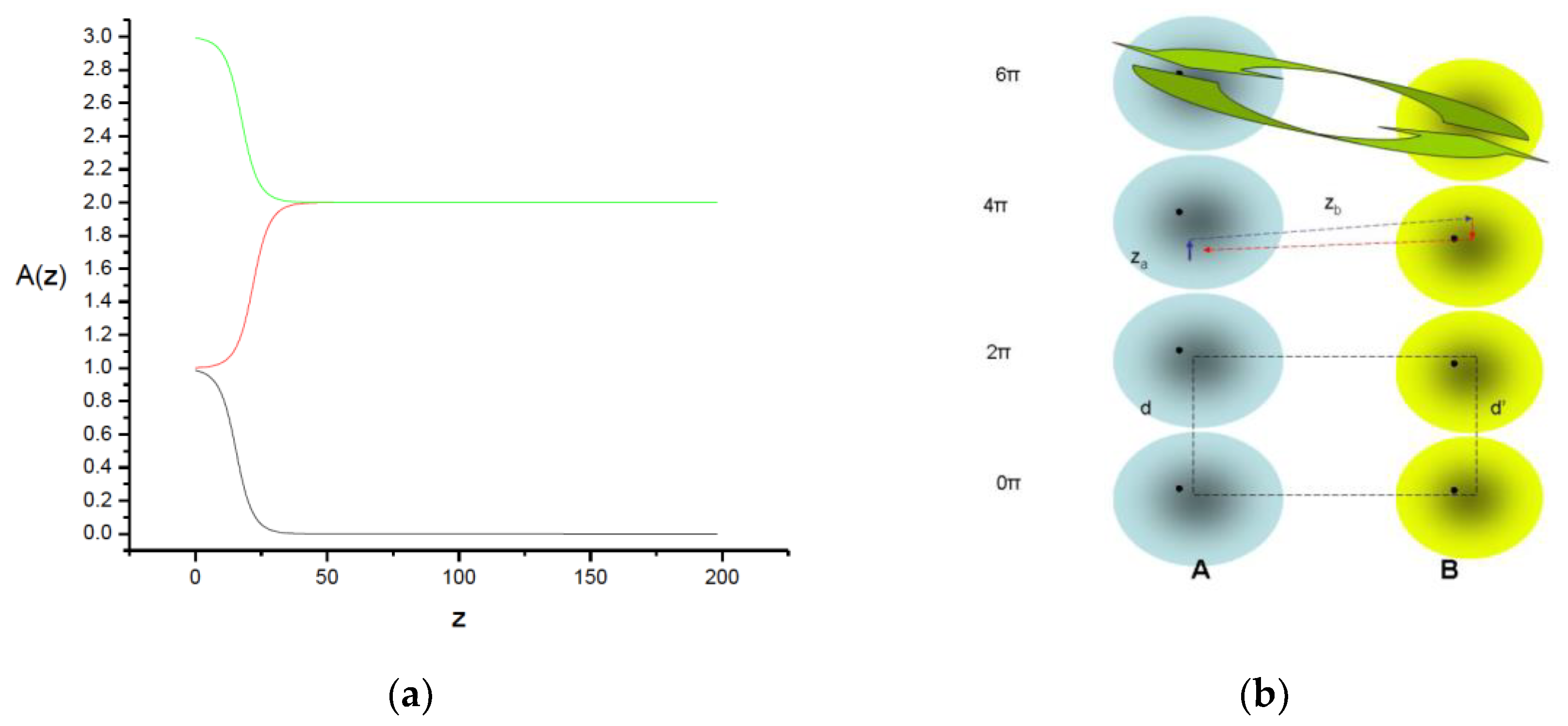
Figure 2.
Area of the pulse as a function of z for . A(z) is in units.
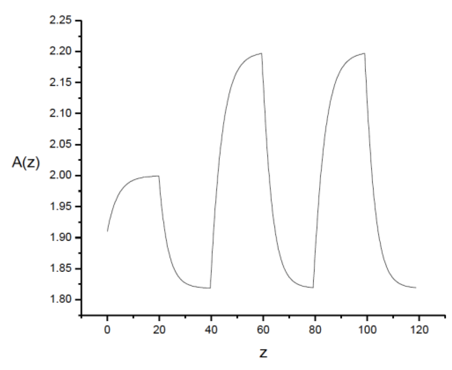
Figure 3.
A The second medium (b) is smaller than the first one and the first remains . A(z) is in units.
Figure 3.
A The second medium (b) is smaller than the first one and the first remains . A(z) is in units.
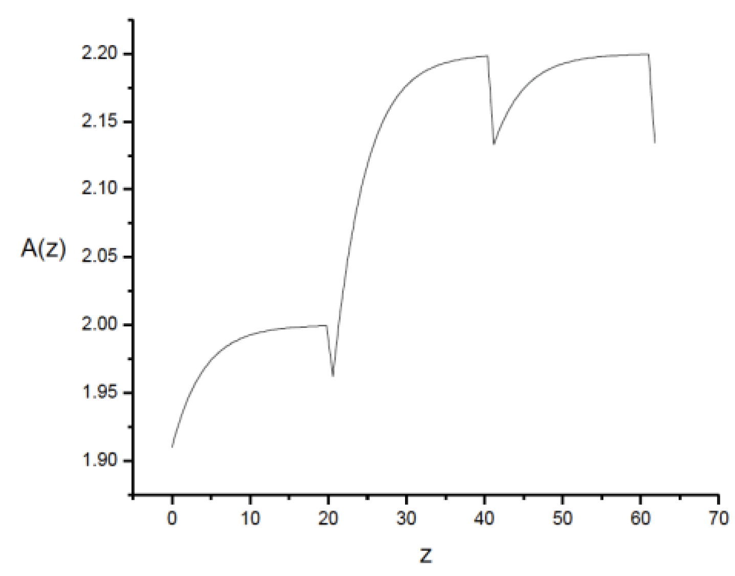
Figure 4.
A The opposite case than the preceding Figure 3: and . A(z) is in units.
Figure 4.
A The opposite case than the preceding Figure 3: and . A(z) is in units.
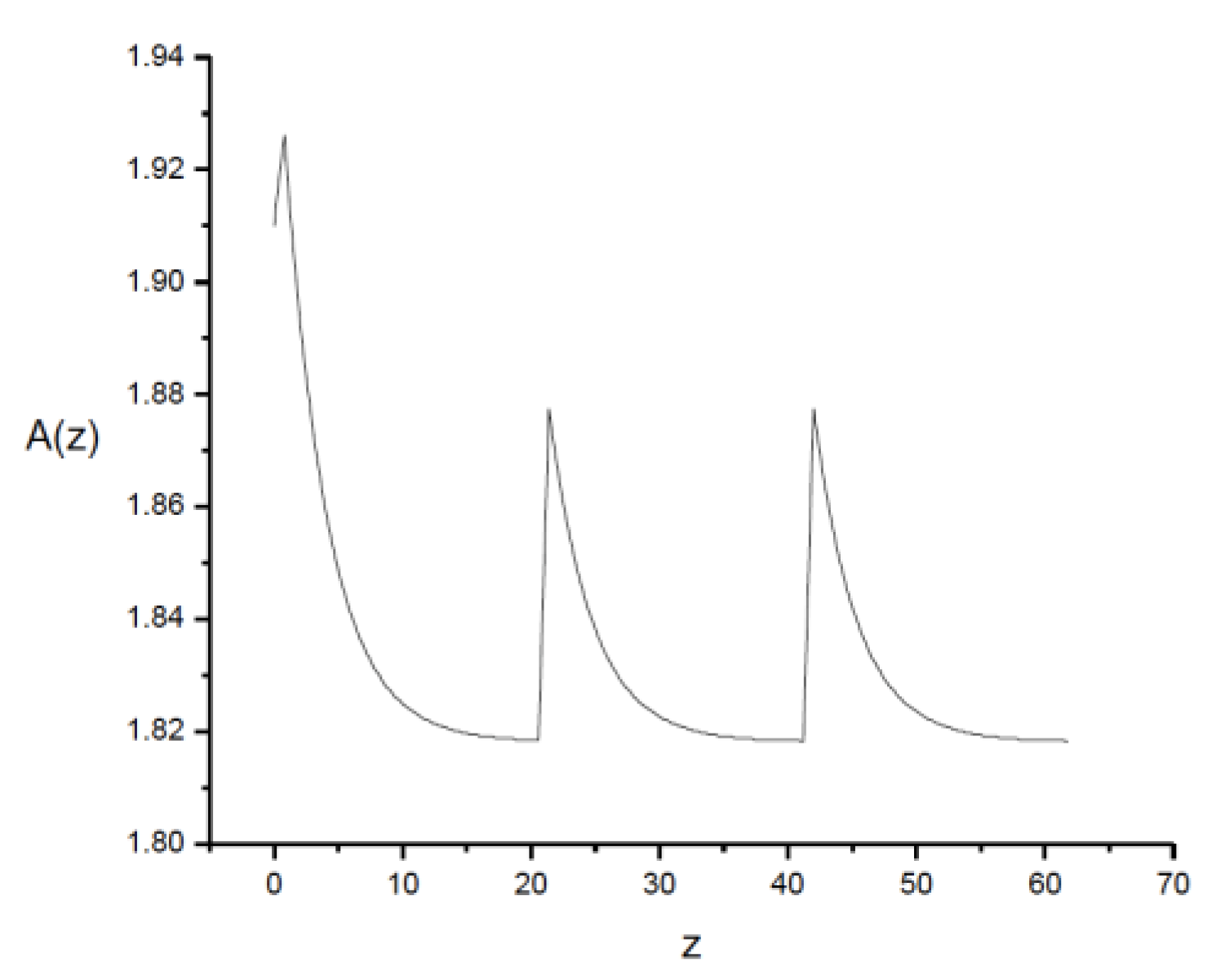
Figure 5.
Both media have a length of only ½ of its inverse , y . A(z) is in units.
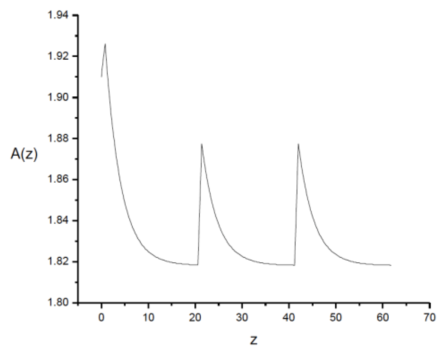
Figure 6.
(a) Propagation of a Kerr soliton in a homogenous material, we can notice the small but visible oscillation in the peak amplitude; (b) The Central peak fluctuations in a homogenous medium are shown in the first column for different . In the second column, we show its Fourier Transform. We can recognize it as a wave number modulation that has a cosenoidal shape, whose period Λ is dependent on the Kerr constant. We selected the period to produce the same number of loops in its Fourier transform for the different and show their dependence on the nonlinearity.
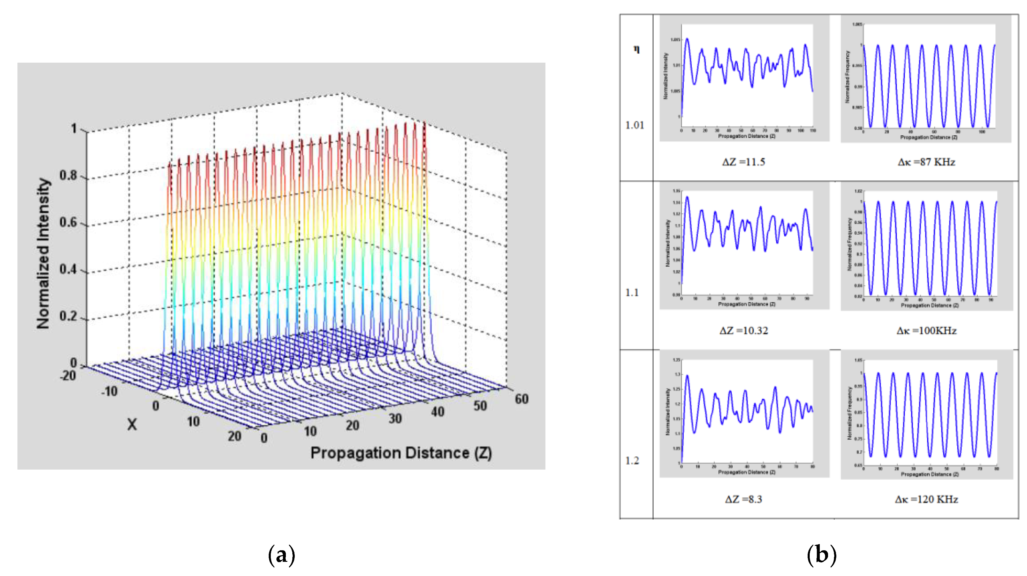
Figure 7.
Propagation in a periodic medium, formed by two Kerr materials with constants and (a) , (b) and (c) . The increasing amplitude of the central peak fluctuations is evident as we increase the difference between the nonlinear coefficients.
Figure 7.
Propagation in a periodic medium, formed by two Kerr materials with constants and (a) , (b) and (c) . The increasing amplitude of the central peak fluctuations is evident as we increase the difference between the nonlinear coefficients.
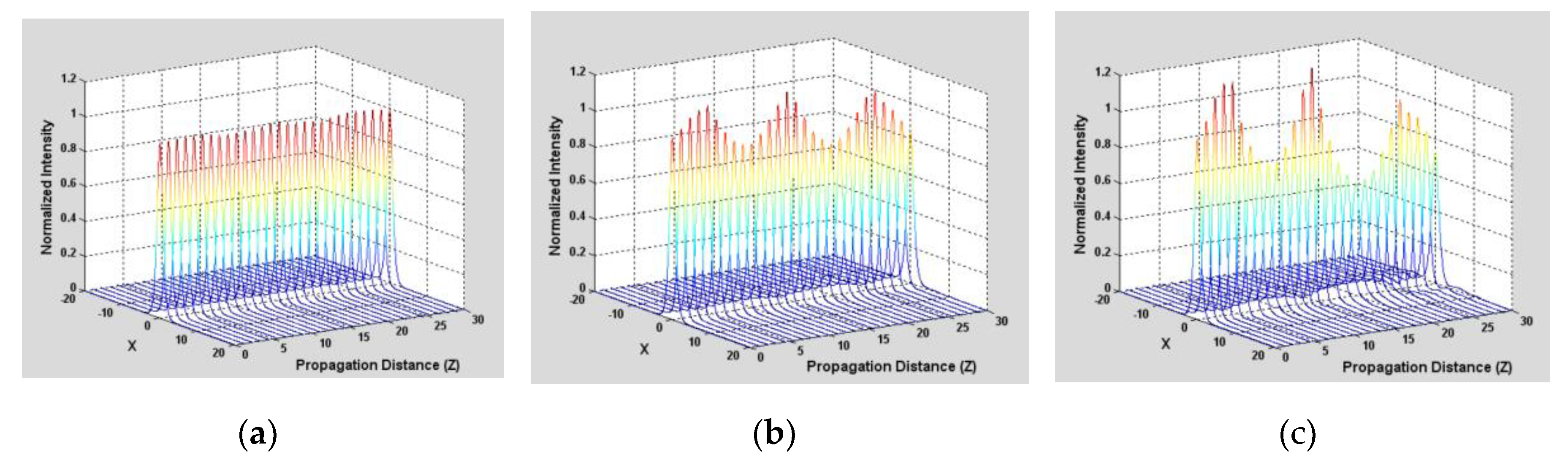
Figure 8.
For the case , we plot this fluctuation as a function of z, from top to bottom rows for the cases described by and (a) , (b) and (c) . and on the columns, from left to right by period thick; and . We can recognize a sawtooth-like reshaping behavior, just as in the resonant case, added to the peak fluctuations whose Λ is large in this case.
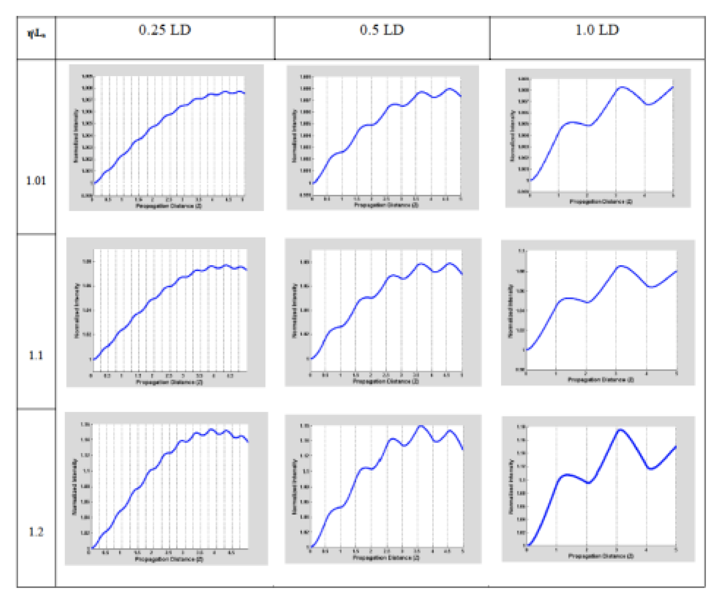
Figure 9.
In the case when , we plot this wave number modulation, from top to bottom rows for the cases described by and (a) , (b) and (c) . and on the columns, from left to right, by thick periods of and . We can notice that Λ is small or comparable to the media modulation.
Figure 9.
In the case when , we plot this wave number modulation, from top to bottom rows for the cases described by and (a) , (b) and (c) . and on the columns, from left to right, by thick periods of and . We can notice that Λ is small or comparable to the media modulation.
Disclaimer/Publisher’s Note: The statements, opinions and data contained in all publications are solely those of the individual author(s) and contributor(s) and not of MDPI and/or the editor(s). MDPI and/or the editor(s) disclaim responsibility for any injury to people or property resulting from any ideas, methods, instructions or products referred to in the content. |
© 2025 by the authors. Licensee MDPI, Basel, Switzerland. This article is an open access article distributed under the terms and conditions of the Creative Commons Attribution (CC BY) license (http://creativecommons.org/licenses/by/4.0/).
Copyright: This open access article is published under a Creative Commons CC BY 4.0 license, which permit the free download, distribution, and reuse, provided that the author and preprint are cited in any reuse.


