
Submitted:
20 August 2025
Posted:
22 August 2025
You are already at the latest version
Abstract
Learning from demonstration with multiple executions must contend with time warping, sensor noise, and alternating quasi stationary and transition phases. We propose a la-bel free pipeline that couples unsupervised segmentation, duration explicit alignment, and probabilistic encoding. A dimensionless multi feature saliency (velocity, acceleration, curvature, direction change rate) yields scale robust keyframes via persistent peak–valley pairs and non maximum suppression. A hidden semi Markov model (HSMM) with ex-plicit duration distributions is jointly trained across demonstrations to align trajectories on a shared semantic time base. Segment level probabilistic motion models (GMM/GMR or ProMP, optionally combined with DMP) produce mean trajectories with calibrated co-variances, directly interfacing with constrained planners. Feature weights are tuned without labels by minimizing cross demonstration structural dispersion on the simplex via CMA ES. Across UAV flight, autonomous driving, and robotic manipulation, the method reduces phase boundary dispersion by 31% on UAV Sim and by 30–36% under monotone time warps, noise, and missing data (vs. HMM); improves the sparsity–fidelity trade off (higher time compression at comparable reconstruction error) with lower jerk; and attains nominal 2σ coverage (94–96%), indicating well calibrated uncertainty. Abla-tions attribute the gains to persistence plus NMS, weight self calibration, and dura-tion explicit alignment. The framework is scale aware and computationally practical, and its uncertainty outputs feed directly into MPC/OMPL for risk aware execution.
Keywords:
hidden semi‑Markov model
; learning from demonstration
; unsupervised segmentation
; feature fusion
; topological persistence
MSC: 68T05
1. Introduction
Learning from Demonstration (LfD) [1] seeks to transfer skills from a handful of expert executions to new task instances. In real deployments across aerial, driving, and manipulation domains, multiple demonstrations routinely exhibit irregular local time warping (hovering, waiting, backtracking) [2,3,4], sensor noise on high-dimensional signals [5,6], and alternating quasi-stationary and transition phases [7,8,9]. Our objective is to discover phase structure without labels, align multiple demonstrations onto a shared semantic time base, and provide calibrated, segment-wise probabilistic models that plug into constrained planners.
A central difficulty is that widely used segmentation and alignment tools either operate at the signal-threshold level or impose duration assumptions that do not reflect how humans actually perform tasks [10,11]. Threshold/template methods or simple peak detectors are brittle to sampling-rate and environment shifts; their decision surfaces move with scale changes, causing under- and over-segmentation in the presence of jitter and speed variations [12,13]. Bayesian online changepoint detection (BOCPD) relieves fixed thresholds but still hinges on hazard-rate and noise assumptions; in practice it often fragments long dwells into multiple short segments when features oscillate, and it provides no explicit duration model for downstream use [14,15,16]. Dynamic Time Warping (DTW) offers pairwise alignment but lacks a generative mechanism and cannot represent dwell distributions or uncertainty, which limits its utility for planning and simulation [17,18,19].
Latent-state models address some of these issues, yet common instantiations come with their own bias-variance trade-offs. Hidden Markov Models (HMMs) assume geometric state durations; this geometric-duration bias shortens non-geometric dwells and shifts boundaries when operators hesitate or loiter, leading to misaligned phases across trials [20]. Hidden semi-Markov Models (HSMMs) are a principled remedy because they explicitly model durations, but most prior pipelines still depend on hand-crafted feature stacks with fixed weights/hyper-parameters, trained per-demonstration or per-session [1,21,22]; robustness degrades under operator/platform shifts and tempo changes. Bayesian nonparametrics can adapt model complexity [23], but the computational overhead and stability concerns have limited their use in long-horizon, multi-demo settings.
Downstream generation has a parallel set of limitations. Dynamical Movement Primitives (DMPs) provide smooth, time-scalable execution but lack closed-form uncertainty; Gaussian Mixture Regression (GMR) and Probabilistic Movement Primitives (ProMPs) offer distributional predictions with covariances, yet both are sensitive to boundary errors—mis-segmentation inflates variances and biases means within segments [20]. More importantly, most pipelines treat segmentation/alignment and probabilistic encoding as loosely coupled stages; there is rarely a mechanism to self-calibrate features using multi-demo consistency or to learn an alignment that is simultaneously scale-aware and duration-aware [24]. Finally, while planners such as OMPL/MPC can exploit covariance for risk-aware control, few works deliver calibrated uncertainty on a shared semantic time base that is directly consumable by these planners [25].
To address these gaps, we propose a label-free pipeline that couples unsupervised segmentation, duration-explicit alignment, and probabilistic encoding into a single, self-calibrating loop. First, we compute a dimensionless multi-feature saliency by fusing velocity, acceleration, curvature, and direction-change rate; then we apply topology-aware keyframe extraction using persistent peak–valley pairs to keep only structurally significant extrema and non-maximum suppression to avoid clustered responses [26]. Second, we jointly train an HSMM across demonstrations with explicit duration distributions and an extended forward–backward recursion, producing a shared semantic time axis and phase-consistent boundaries [25]. Third, within each phase we fit probabilistic motion models—GMM/GMR or ProMP, optionally combined with DMP for execution—to obtain mean trajectories with calibrated covariances [20]. Crucially, we close the loop by learning the saliency weights without labels: a CMA-ES [27] search on the probability simplex minimizes cross-demonstration structural dispersion, automatically rebalancing features so that segmentation and alignment are mutually consistent. Compared with BOCPD, thresholding, or HMM-based pipelines, this design is explicitly duration-aware, scale/time-warp robust, and planner-ready with uncertainty that is calibrated and comparable across operators.
Contributions.
- Scale-/time-warp-robust saliency. A topology-aware, multi-feature saliency (persistence and non-maximum suppression) that stabilizes keyframes under noise and tempo variations, yielding sparser yet more stable anchors than signal-level detectors.
- Joint HSMM alignment with explicit durations. Cross-demo training with extended forward–backward/Viterbi recursions; model order selected by a joint criterion combining BIC and alignment error (AE) to balance fit and parsimony.
- Label-free feature-weight self-calibration. CMA-ES on the weight simplex to minimize cross-demo structural dispersion, eliminating hand-tuned fusion and improving phase consistency.
- Calibrated probabilistic encoding for planning. Segment-wise GMR/ProMP (optionally fused with DMP) returning means and covariances that integrate directly with OMPL/MPC for risk-aware execution.
Empirically, on UAV flight, autonomous-driving, and manipulation benchmarks, our method reduces phase-boundary dispersion by ≈31% on UAV-Sim and by 30–36% under monotone time warps, additive noise, and missing data compared with HMM variants; it improves the sparsity–fidelity–smoothness trade-off (higher time compression at comparable reconstruction error with lower jerk) and achieves nominal 2σ coverage (94–96%), indicating well-calibrated uncertainty. Section 2 details the pipeline; Section 3 reports datasets, metrics, baselines (including BOCPD and HMM), ablations, and robustness; Section 4 discusses positioning, limitations, and future work; Section 5 concludes.
2. Materials and Methods
Figure 1 sketches the end-to-end workflow that maps multiple demonstrations to executable trajectories under physical and safety constraints: (i) unsupervised segmentation from multi-feature saliency with topology-aware keyframes; (ii) duration-explicit alignment across demonstrations via a hidden semi-Markov model (HSMM) with shared parameters; and (iii) probabilistic encoding of each phase (GMM/GMR or ProMP, optionally combined with DMP) producing mean trajectories with calibrated covariances. Outputs include phase-consistent labels, segment-wise probabilistic models, and constraint-aware executable trajectories.
2.1. Inputs, Outputs, and Assumptions
- Inputs.
We observe M independent demonstrations (optionally multi-modal), sampled with fixed period . When available, auxiliary channels (e.g., pose, force/tactile, depth) are concatenated into the observation vector used downstream.
- Outputs.
A shared set of semantic phases and per-demo boundaries ;
For each phase, a segment-wise generative model—DMP, GMM/GMR, or ProMP, alone or in combination—returning mean trajectories and covariance estimates;
Under constraints (terminal/waypoints, velocity/acceleration limits, etc.), an executable trajectory and associated risk measures computed from covariances.
- Assumptions.
- Demonstrations consist of alternating quasi-stationary and transition segments.
- Time deformation is order-preserving (the semantic phase order does not change).
- Observation noise is moderate and can be mitigated by local smoothing and statistical filtering.
2.2. Multi-Feature Analysis and Automatic Segmentation
2.2.1. Data Ingestion and Pre-modulation
Let a single demonstration be the discrete sequence , where is the number of observed degrees of freedom (e.g., for UAV or mobile bases; for industrial manipulators). Cumulative sums yield the Cartesian trajectory of the tool center point
We apply a one-dimensional Savitzky–Golay local polynomial smoother to before computing derivatives, suppressing high-frequency tele-operation jitter and stabilizing numerical differentiation. The filter is equivalent to an -order Taylor truncation in time and ensures
Implementation note. Central differences are used for derivatives; all channels are time-synchronized at a fixed sampling period .
2.2.2. Feature Computation and Saliency Fusion
On the smoothed trajectory we compute four complementary, time-varying features that reveal when, where, and how kinematic changes occur ( is fixed).
- Velocity. Let
- 2.
- Acceleration.
Peaks indicate abrupt speed changes.
- 3.
- Curvature. With ΔP(t)=P(t+1)-P(t),
Curvature measures spatial bending and is naturally invariant to global time scaling due to the cubic velocity term [29,30].
- 4.
- Direction-Change Rate (DCR). Define the unit-direction vector . To avoid numerical issues at very low speed, introduce a threshold and set
- 5.
- Dimensionless fusion. Apply min–max normalization to each feature to obtain . For a weight vector with and , define the fused saliency
The weights are learned without labels in Section 2.2.4.
2.2.3. Keyframe Extraction with Topological Simplification
The saliency compresses multi-source information into a 1-D signal, but segmentation should rely on structural extrema (global landmarks), not every minor fluctuation. We adopt a bottom-up screening that contracts a dense set of local extrema into a sparse, stable keyframe set [1,31].
- Candidate extrema via quantile thresholds.
Let be a grid of quantiles (e.g., uniformly in [0.60,0.95]). For each :
- set ;
- collect indices and snap each to the nearest local extremum within a radius-3 neighborhood.
To pick a unique , minimize a sparsity–fidelity loss
- 2.
- Persistence thresholding (scale-invariant importance).
For adjacent peak–valley pairs of , define the persistence
Small persistence typically indicates noise or micro-tremor; large persistence corresponds to genuine kinematic transitions. Plot
Because persistence depends only on amplitude differences, it is invariant to vertical scaling and mild time stretching, facilitating cross-demo comparability [32,33].
- 3.
- Non-maximum suppression (NMS).
To avoid peak clustering, scan with a sliding window of frames and retain an extremum only if it is the largest (same polarity) within the window. The final keyframe set is
The effect of persistence thresholding and NMS is illustrated in Figure 2, which contracts dense peak clusters into a sparse, stable keyframe set . The black solid curve is the original saliency signal ; the dashed curve is the simplified signal after persistence-based filtering (elbow detected by Kneedle) and non-maximum suppression (window ). Green crosses mark the final retained keyframes . The procedure removes clustered minor extrema while preserving structural landmarks that drive segmentation and alignment.
With in place, the reliability of subsequent segmentation and HSMM alignment still depends on the saliency weights ; Section 2.2.4 details a label-free, consistency-driven calibration.
2.2.4. Adaptive Feature-Weight Learning
In (2.6), the saliency is a linear fusion of four heterogeneous features. Assigning heuristic, fixed weights typically overfits a particular operator, platform, or task, degrading segmentation under distribution shift. We therefore treat as model parameters to be estimated without labels by enforcing cross-demonstration consistency.
- Consistency functiona.
For demonstrations and a candidate , define
denote the composition of saliency construction, keyframe extraction (Figure 2), HSMM-based alignment (Section 2.3), and resampling on shared semantic nodes. If is well chosen, the reconstructions should be congruent in shape and timing. We quantify this by the mean point-to-point structural dispersion.
here is the minimal resampled length. Smaller SOD means lower structural variance on the shared semantic time base.
- 2.
- Objective and constraints.
To prevent dominance by any single channel and to improve identifiability, we regularize with a light penalty and minimize over the probability simplex:
Because F contains non-smooth steps (extrema detection, discrete decoding), is non-differentiable and gradient methods are unreliable.
- 3.
- Solver and feasibility.
We employ the Covariance Matrix Adaptation Evolution Strategy (CMA-ES) in an unconstrained space together with a softmax reparameterization
- 4.
- Computational profile.
Each evaluation of entails one pass of keyframe extraction (linear in sequence length ) and one HSMM forward–backward/decoding pass per demonstration with complexity ; overall cost scales linearly in . For numerical stability we implement recursions in the log domain (log-sum-exp), apply a diagonal floor to GMM covariances, and cache feature streams across outer-loop calls.
2.3. Multi-Demo Alignment and Segmentation via a Duration-Explicit HSMM
Given the sparse, scale-invariant keyframes obtained from saliency (Section 2.2) and the learned fusion weights (Section 2.2.4), we seek a shared semantic time base across demonstrations. Directly matching wall-clock indices is unreliable due to operator-dependent pauses and backtracking; instead, we align demonstrations probabilistically via a Hidden semi-Markov model (HSMM) that explicitly models state durations (Figure 3) [37,38].
2.3.1. Model and Generative Mechanism
Let be latent phases, each representing a macro-action (e.g., grasp, insert, lift). With parameters , the HSMM generates at as follows:
- a)
- Initial phase:
- b)
- Duration: for the current phase , sample dwell length .
- c)
- Observations: for with ,
- d)
- Transition: ; terminal transitions end the sequence.
Writing and for , the joint density is
- Observation design. We concatenate kinematic descriptors (e.g., curvature, speed magnitude, DCR) and any available modalities (pose, force/tactile, depth) into .
- Duration choices. We use either discrete with support 1: , or truncated Gaussian/Gamma families to accommodate unequal dwell times [39].
2.3.2. Parameter Estimation: Extended Baum–Welch
We maximize the total log-likelihood over demonstrations
Explicit durations break first-order Markovity; forward–backward recursions therefore enumerate duration indices.
- 1.
- Forward variable (leaving at time ).
- 2.
- Backward variable.
- 3.
- Posteriors (E-step).
Sum over to obtain corpus-level sufficient statistics.
- 4.
- M-step (closed forms).
- 5.
-
Numerical stability.All recursions are implemented in the log domain using log-sum-exp
2.3.3. Semantic Time Axis: Decoding and Outputs
After convergence, Viterbi decoding yields the MAP phase path and durations for each demonstration, with . Define cumulative boundaries , so segments correspond to the same semantic phase across demonstrations. Figure 4 and Figure 5 illustrate 3-D keyframe locations and HSMM reconstructions aligned to salient kinematic transitions.
2.3.4. Alignment Quality, Model Selection, and Robustness
Alignment metric. We quantify cross-demo temporal agreement by
Model selection. To balance fit and parsimony, we use
and select by jointly considering and .
Robustness to time warps. For any order-preserving reparameterization of time, , the decoded phase order is invariant; only the tail behavior of duration distributions is rescaled. This accounts for operator-dependent slowdowns, hesitations, or hovering.
Complexity. Keyframe processing is per sequence; duration-explicit forward–backward is ; training scales linearly in the number of demonstrations M. Outputs include , and segment-wise statistics for direct use by planners (e.g., OMPL/MPC).
2.4. Statistical Motion Primitives and Probabilistic Generation
With cross-demonstration phases and boundaries , obtained from the duration-explicit HSMM (Section 2.3), we model each phase within the shared semantic time base. For demonstration , let
2.4.1. Dynamic Movement Primitives (DMP)
- Single-segment dynamics.
For a one-degree-of-freedom trajectory , the classical DMP represents motion as a critically damped second-order system with a nonlinear forcing term:
where is the segment goal, is a phase variable, and
Given the weights are obtained by least squares (or locally weighted regression). Multi-DOF trajectories are modeled component-wise or via task-space coupling.
- 2.
- Segment coupling and smoothness.
Let be the mean duration of phase across demonstrations; set . We fit per segment and compose along the decoded boundaries. Because the state is continuous across boundaries, the concatenation is -continuous without auxiliary velocity/acceleration matchers. DMPs thus offer low jerk and robust time-scaling at execution.
2.4.2. Gaussian Mixture Modeling and Regression (GMM/GMR)
Mixture modeling. For each segment, we pair normalized phase with position, , and fit a K-component mixture
typically with diagonal (or block-diagonal) to denoise while retaining principal correlations.
Regression and uncertainty. At execution, Gaussian Mixture Regression (GMR) produces the conditional
2.4.3. Probabilistic Movement Primitives (ProMP)
Bayesian representation. Using basis functions , a segment trajectory is modeled as
where encode the distribution over shapes learned from multiple demonstrations (EM or closed-form under Gaussian assumptions).
Conditioning and coordination. Linear constraints—endpoints, waypoints, or partial observations—are imposed by conditioning the weight distribution:
with . Sampling from this posterior and stitching segments at decoded boundaries yields constraint-consistent trajectories with explicit predictive uncertainty.
2.4.4. Model Choice and Complementarity
No single primitive dominates: DMP excels in real-time low-jerk execution; GMM/GMR gives closed-form means/covariances and gradients; ProMP supports exact linear-Gaussian conditioning for multi-goal tasks. Table 1 summarizes properties. Figure 6 shows HSMM-aligned ProMP generation with calibrated uncertainty bands:
- DMP excels at real-time execution and low jerk with simple time scaling;
- GMM/GMR offers closed-form means and covariances over phase and is convenient for planners needing analytic gradients;
- ProMP provides a distribution over shapes with exact linear-Gaussian conditioning, ideal for multi-goal tasks and collaboration.
In practice, we first fit GMM/GMR to obtain mean/covariance; use the GMR mean to initialize DMP weights for smooth execution; and, when hard/soft constraints or multi-goal adaptation are required, overlay ProMP conditioning on top of the DMP nominal to reconcile smoothness with constraints.
Interface to planning and safety. Segment-wise covariances (from GMR or ProMP) propagate to risk metrics and constraint tightening in MPC/OMPL. Because segments share a semantic time base, the uncertainty is comparable across operators and platforms, enabling principled safety margins (e.g., envelopes) and priority-aware blending when composing multi-segment tasks.
Computational profile. Per segment, DMP fitting is linear in the number of basis functions; GMM/GMR training is per EM iteration; ProMP estimation is closed-form/EM with state dimension B. Since segments are independent given HSMM alignment, training parallelizes over phases and scales linearly with the number of demonstrations.
3. Experiments and Results
3.1. Objectives and Evaluation Protocol
This section subjects the proposed end-to-end pipeline to a cross-domain, reproducible evaluation covering the three core components introduced in Section 2: (i) unsupervised segmentation (multi-feature saliency with topological persistence), (ii) duration-explicit alignment (HSMM), and (iii) probabilistic in-segment generation (GMM/GMR, ProMP, optionally DMP). We target three complementary questions:
- Segmentation robustness. Do multi-feature saliency and topological persistence yield sparse yet structurally stable keyframes under heterogeneous noise and tempo variations?
- Semantic alignment quality. Does duration-explicit HSMM reduce cross-demonstration time dispersion when non-geometric dwelling is present (e.g., hover, wait)?
- Generator calibration. On the shared semantic time base, do segment-wise probabilistic models achieve low reconstruction error, nominal uncertainty coverage, and dynamically schedulable executions?
To mitigate methodological contingency, we span diverse dynamics, perturbations, and baselines, and we control for multiple comparisons in statistical inference.
3.2. Tasks, Datasets, and Testable Hypotheses
We consider three representative domains:
- Domain A—UAV-Sim (multi-scene flight). 100 Hz sampling. Subtasks include take-off–lift–cruise–drop and gate-pass–loiter–gate-pass. Six subjects, 20–30 segments per task. Observations: tool-center position (optional yaw). Figure 7 shows the environment and demonstrations.
- Domain B—AV-Sim (CARLA/MetaDrive urban). 10 Hz sampling across Town01–05, varied weather/lighting and traffic control. Trajectories originate from an expert controller and human tele-operation. Observations: . See Figure 8.
- Domain C—Manip-Sim (robomimic/RLBench assembly). 50–100 Hz sampling. Tasks akin to RoboTurk “square-nut”: grasp–align–insert with pronounced dwell segments. Observations: end-effector position. See Figure 9.
3.3. Metrics and Statistical Inference
We harmonize five dimensions—structure, time, geometry, dynamics, probability—using the following metrics (units: meters for UAV/AV, millimeters for Manip-Sim; each table caption clarifies units). Unless otherwise noted, SOD, AE, GRE, and Jerk are minimized; TCR and AAR are maximized; CR targets 95%.
- SOD (Eq. (2.10), min): structural dispersion—mean point-to-point divergence on the shared time base.
- AE (Eq. (2.17), min): Euclidean dispersion of phase end times across demonstrations.
- AAR (max): action acquisition rate. Given reference key actions (expert consensus / common boundaries) and detected , we count a hit if , with (i.e., 50 ms at 100 Hz; 0.5 s at 10 Hz).
- GRE (min): geometric reconstruction error (RMSE).
- TCR (max): time compression rate.
- Jerk (min): (normalized).
- CR (target ≈ 95%): nominal coverage. For each semantic segment we sample uniformly in time; if , it is counted as covered; segment-level coverage is averaged and then length-weighted globally.
Statistical inference. We apply Shapiro–Wilk normality and Levene homoscedasticity tests. When met, paired t-tests are used; otherwise Wilcoxon signed-rank tests. Multiple comparisons are controlled via Holm–Bonferroni. We report p-values, Cohen’s d, and BCa 95% bootstrap confidence intervals (1,000 resamples).
3.4. Baselines and Fairness Controls
We benchmark four families to isolate contributions at the signal, boundary, and latent levels:
(i) Signal-level: single-feature curvature + quantile threshold; and multi-feature equal weights without TDA simplification / NMS (no persistence, no cluster suppression).
(ii) Boundary-level: BOCPD (Bayesian Online Changepoint Detection).
(iii) Latent-level: multi-feature + TDA/NMS + HMM (geometric duration assumption).
(iv) Full method: (consistency-learned weights) + TDA/NMS + HSMM (duration explicit) + segment-wise generator (default ProMP; we also compare DMP/GMR on the same segmentation when isolating generation quality, § 3.9).
Fairness controls. All methods share identical preprocessing (uniform sampling, same-order Savitzky–Golay smoothing, consistent derivative computation, per-trajectory min–max normalization), model-selection strategy (BIC+AE; same candidate sets for GMM components), and EM initialization/termination. Segmentation quality is evaluated using each model’s MAP/Viterbi boundaries; for pure generator comparison (§ 3.9), we fix HSMM boundaries across methods to remove boundary confounds.
3.5. Overall Results
Cross-domain evidence appears in Figure 10 and Table 2. Figure 10a overlays multiple demonstrations in 3D; Figure 10(b) shows curvature, velocity, acceleration, direction-change, and their fused saliency for one trajectory. Peaks co-occur at kinematic turning points, and the fused saliency forms stable spikes at these locations—explaining the high keyframe consistency across subjects and durations.
- Domain A—UAV-Sim (Table 2)
In subtasks with hover/backtrack dwell, introducing HSMM reduces AE from s to s (−31%, p < 0.01, Cohen’s ). With comparable GRE, TCR increases by 10–12 pp and Jerk decreases, indicating a better sparsity–fidelity–smoothness trade-off. The probabilistic output attains CR ≈ 95% at the nominal level.
- Domain B—AV-Sim (Table 3)
In segments with non-geometric dwell (e.g., slow-down–wait–turn), AE drops from s under HSMM; SOD and GRE decrease in tandem, indicating reduced in-segment statistical bias. ProMP coverage at is .

Table 3.
AV-Sim (CARLA/MetaDrive) (units: SOD/GRE in meters).
| Method | SOD (m) | AE (s) | GRE (m) | TCR (%) | AAR (%) | Jerk | CR (%) |
|---|---|---|---|---|---|---|---|
| Curvature + quantile | 0.172 ± 0.030 | 0.70 ± 0.14 | 0.247 ± 0.041 | 32.7 ± 5.2 | 66.0 ± 6.7 | 1.18 ± 0.09 | – |
| Multi-feat (equal), no TDA/NMS | 0.160 ± 0.029 | 0.63 ± 0.12 | 0.231 ± 0.038 | 39.5 ± 5.0 | 71.6 ± 6.1 | 1.14 ± 0.08 | – |
| Multi-feat + TDA/NMS + HMM | 0.148 ± 0.027 | 0.55 ± 0.11 | 0.214 ± 0.035 | 47.4 ± 4.7 | 78.8 ± 5.4 | 1.08 ± 0.07 | – |
| Ours: +TDA/NMS+HSMM+ProMP | 0.112 ± 0.022 | 0.37 ± 0.08 | 0.191 ± 0.033 | 47.5 ± 4.6 | 86.3 ± 5.0 | 1.00 ± 0.06 | 95.1 ± 2.5 |
- Domain C—Manip-Sim (Table 4)
Dwell-heavy phases (grasp/insert) strongly expose non-geometric duration. The full method improves SOD, AE, and TCR over signal thresholds, HMM, and BOCPD; notably, it achieves higher TCR at comparable or lower GRE, i.e., fewer keyframes suffice to reconstruct high-fidelity shapes.
Table 4.
Manip--Sim (robomimic/RLBench) (units: SOD/GRE in millimeters).
| Method | SOD (mm) | AE (s) | GRE (mm) | TCR (%) | AAR (%) |
|---|---|---|---|---|---|
| Curvature + quantile | 1.12 ± 0.27 | 0.33 ± 0.09 | 1.02 ± 0.19 | 30.0 ± 4.8 | 65.3 ± 6.3 |
| Multi-feat (equal), no TDA/NMS | 0.94 ± 0.24 | 0.28 ± 0.08 | 0.86 ± 0.16 | 33.0 ± 5.0 | 69.1 ± 5.8 |
| Multi-feat + TDA/NMS + HMM | 0.87 ± 0.22 | 0.29 ± 0.08 | 0.91 ± 0.17 | 35.1 ± 5.1 | 70.0 ± 5.7 |
| BOCPD | 0.98 ± 0.25 | 0.31 ± 0.09 | 1.05 ± 0.20 | 45.0 ± 5.6 | 71.9 ± 5.4 |
| Ours: +TDA/NMS+HSMM +ProMP |
0.72 ± 0.18 | 0.24 ± 0.07 | 0.79 ± 0.15 | 49.2 ± 4.8 | 83.4 ± 5.1 |
Semantic time alignment. As shown in Figure 11, velocity peaks are misaligned on the physical time axis (a), but become synchronized on the semantic axis after HSMM (b); dashed lines (phase boundaries) nearly coincide across demonstrations. This mirrors the systematic AE reduction in Table 2, Table 3 and Table 4 and evidences the benefit over geometric-duration HMM.
3.6. Contribution Attribution: Ablation Study (UAV-Sim)
We perform stepwise ablations under LOSO with (other settings as in § 3.3–3.4). Table 5 reports relative changes w.r.t. the full method (+TDA/NMS+HSMM+ProMP); positive values are worse (e.g., AE↑), negative better.
- Remove TDA (keep NMS): SOD +12.3%, AE +9.6% → persistence is key to scale-invariant noise rejection; without it, small-scale oscillations stack into spurious peak–valley pairs, degrading structure and boundaries.
- Remove NMS (keep TDA): AE +21.1% → suppressing same-polarity peak clusters in high-energy regions is critical for boundary stability; persistence alone cannot prevent multi-response.
- Fix equal weights (no ): SOD +18.6%, AAR −7.7 pp → consistency-driven weight learning mitigates channel scale imbalance and improves key-action capture.
- Replace HSMM with HMM: AE +31.2% → direct evidence of the geometric-duration bias when dwell exists (wait/loiter).
Differences on AE and SOD remain statistically significant after Holm–Bonferroni (p < 0.05); effect sizes are medium-to-large. In sum: TDA+NMS stabilize the input structure, provides cross-demo self-calibration, and HSMM addresses duration bias mechanistically.
3.7. Robustness: Time-Warping, Noise, and Missing Data (AV-Sim)
We evaluate robustness on AV-Sim (Table 6. We apply monotone time warps (speed-up) and (slow-down), add white noise to positions, and randomly drop 20% of samples. Compared to HMM, HSMM reduces AE by 36%, 34%, 30%, and 35%, respectively, while preserving phase order. AE grows roughly linearly with noise amplitude but, under order-preserving time warps, manifests mainly as duration redistribution—consistent with the “weak time-distortion invariance” discussed in § 2.4.
ProMP coverage stays within 94–96% under these perturbations, indicating stable uncertainty calibration.
3.8. Model Selection and the Sparsity–Fidelity Trade-off
Figure 12 shows how the persistence threshold controls keyframe sparsity and reconstruction GRE. As increases, keyframe count decreases monotonically; GRE stabilizes near the Kneedle elbow (vertical dashed line), reflecting an effective sparsity–fidelity compromise with BCa 95% CIs (shaded).
To determine HSMM state number , we train models on with identical hyper-parameters and initialization. On the validation set we compute AE and BIC (Eq. (2.17) and Eq. (2.20)), normalize both to , and average across subjects. Figure 13 shows that AE decreases rapidly then plateaus at , whereas BIC increases monotonically. The joint criterion yields the optimal number of states or UAV/AV and 5 for Manip-Sim (star markers). Deviating by ±1 does not change the overall trend; we fix in all experiments to balance alignment accuracy and parsimony.
3.9. In-Segment Generation: Accuracy, Smoothness, and Calibration
On a fixed semantic time base we compare linear interpolation, DMP, GMR, and ProMP (Figure 14):
- Geometry: ProMP ≈ GMR < DMP < linear in GRE.
- Smoothness: DMP minimizes Jerk, suiting online execution and hard real-time constraints.
- Calibration: ProMP/GMR achieve CR = 94–96% at the nominal 95%, with small reliability-curve deviations—amenable to MPC/safety monitoring.
Segments are concatenated at HSMM boundaries with continuity (see Eqs. (2.19)–(2.20)); the critically damped second-order dynamics preserve velocity/acceleration continuity across segments.
3.10. Summary of Findings
We presented an end-to-end trajectory-learning framework for multiple demonstrations. Unsupervised multi-feature saliency with topological persistence yields stable segmentation; HSMM with explicit durations delivers robust cross-demo semantic alignment; ProMP/GMR (optionally fused with DMP) enable probabilistic generation with smooth execution. Across UAV/AV/Manip tasks, the method consistently outperforms representative baselines (single-feature thresholds, BOCPD, HMM) on AE, SOD, AAR, and the sparsity–fidelity trade-off, and remains robust to time-warping, noise, and missing data. Unlike prior templates or manual labels, weights are learned via consistency-driven optimization, and outputs include calibrated uncertainties directly consumable by MPC/OMPL. In sum, the framework remedies geometric-duration bias and the “segmentation–encoding split,” enabling accurate modeling and faithful reproduction of complex trajectories—ready for industrial tasks such as polishing, coating, welding, assembly, and autonomous driving paths.
4. Discussion
- Evidence vs. hypotheses.
- (H1) Segmentation. The topology-aware saliency (multi-feature + persistence + NMS) yields sparse yet stable anchors: removing persistence or NMS increases SOD/AE by 9–21% and lowers AAR (ablation), confirming that both scale-invariant pruning and peak-cluster suppression are necessary.
- (H2) Alignment. Duration-explicit HSMM reduces phase-boundary dispersion (AE) by 31% in UAV-Sim and by 30–36% under time warps, noise, and missing data relative to HMM/BOCPD; misaligned velocity peaks synchronize on the semantic axis, evidencing mitigation of geometric-duration bias.
- (H3) Generation. On the shared semantic time base, ProMP and GMR achieve low GRE and nominal 2σ coverage (94–96%), while DMP minimizes jerk; higher TCR at comparable GRE indicates a better sparsity–fidelity trade-off.
Positioning to prior work. Rule- or template-based segmentation and BOCPD lack geometric/semantic guarantees; DTW aligns sequences but offers no generative dwell model; HMMs assume geometric durations. Our joint HSMM training across demonstrations, coupled with consistency-driven weight learning, provides phase semantics with explicit duration distributions and avoids hand-tuned weights.
Practical implications. Segment-wise covariances (GMR/ProMP) propagate directly to MPC/OMPL for risk-aware execution; the entire pipeline is label-free and computationally linear in the number of demonstrations; Figure 12 and Figure 13 give operational choices for the persistence threshold and state number.
Limitations. (i) Weakly featured tasks may yield shallow saliency peaks; (ii) the fixed feature family can miss critical modalities (e.g., tactile); (iii) unimodal duration models may underfit multi-modal dwell; (iv) Kneedle/NMS windows are still heuristics; (v) sim-to-real effects may perturb calibration.
Future work. Learn saliency representations with topological regularization; develop differentiable surrogates for persistence/NMS and variational HSMMs; adopt richer (hierarchical or hazard-based) duration processes; enable online EM and adaptive ProMP/GMR updates; integrate with chance-constrained/CBF-MPC; extend to multi-agent coordination on the semantic time base.
5. Conclusions
We introduced a label-free pipeline that (i) extracts scale-robust keyframes via topology-aware multi-feature saliency, (ii) performs duration-explicit alignment with a jointly trained HSMM to build a shared semantic time base, and (iii) encodes each phase probabilistically (GMR/ProMP, optionally combined with DMP) for smooth, risk-aware execution. Across UAV, AV, and manipulation domains the method cuts AE by 31% (UAV-Sim) and 30–36% under perturbations, improves the sparsity–fidelity trade-off (higher TCR at similar GRE) with lower jerk, and attains nominal 2σ coverage (94–96%). The approach resolves geometric-duration bias and the segmentation–encoding split, and its calibrated uncertainties interface directly with MPC/OMPL. Remaining gaps—feature set, duration richness, and sim-to-real transfer—motivate future work on learned representations, richer dwell models, and online adaptation for safety-critical deployment.
Author Contributions
Conceptualization, T.G., K.A.N., and D.D.D.; Methodology, T.G. and K.A.N.; Software, T.G.; Validation, B.Y. and S.R.; Formal analysis, T.G.; Investigation (experiments), T.G., B.Y., and S.R.; Data curation, T.G., B.Y., and S.R.; Visualization, T.G.; Writing—original draft, T.G.; Writing—review & editing, K.A.N., D.D.D., and T.G.; Supervision, K.A.N. and D.D.D.
Funding
This work was supported by the China Scholarship Council (CSC) under the “Russia Talent Training Program”, under Grant 202108090390. (Corresponding author: Gao Tianci).
Data Availability Statement
The original contributions presented in this study are included in the article. Further inquiries can be directed to the corresponding author.
Conflicts of Interest
The authors declare no conflicts of interest.
References
- Correia, A.; Alexandre, L.A. A survey of demonstration learning. Robotics and Autonomous Systems 2024, 182, 104812. [Google Scholar] [CrossRef]
- Jin, W.; Murphey, T.D.; Kulić, D.; et al. Learning from sparse demonstrations. IEEE Transactions on Robotics 2022, 39, 645–664. [Google Scholar] [CrossRef]
- Lee, D.; Yu, S.; Ju, H.; et al. Weakly supervised temporal anomaly segmentation with dynamic time warping. In Proceedings of the IEEE/CVF International Conference on Computer Vision (ICCV); 2021; pp. 7355–7364. [Google Scholar]
- Braglia, G.; Tebaldi, D.; Lazzaretti, A.E.; et al. Arc--length--based warping for robot skill synthesis from multiple demonstrations. arXiv 2024, arXiv:2410.13322. [Google Scholar]
- Si, W.; Wang, N.; Yang, C. A review on manipulation skill acquisition through teleoperation--based learning from demonstration. Cognitive Computation and Systems 2021, 3, 1–16. [Google Scholar] [CrossRef]
- Arduengo, M.; Colomé, A.; Lobo--Prat, J.; et al. Gaussian--process--based robot learning from demonstration. Journal of Ambient Intelligence and Humanized Computing 2023, 1–14. [Google Scholar] [CrossRef]
- Tavassoli, M.; et al. Learning skills from demonstrations: A trend from motion primitives to experience abstraction. IEEE Transactions on Cognitive and Developmental Systems 2023, 16, 57–74. [Google Scholar] [CrossRef]
- Ansari, A.F.; Benidis, K.; Kurle, R.; et al. Deep explicit duration switching models for time series. In Advances in Neural Information Processing Systems (NeurIPS); 2021; 34, 29949–29961.
- Sosa--Ceron, A.D.; Gonzalez--Hernandez, H.G.; Reyes--Avendaño, J.A. Learning from demonstrations in human–robot collaborative scenarios: A survey. Robotics 2022, 11, 126. [Google Scholar] [CrossRef]
- Ruiz--Suarez, S.; Leos--Barajas, V.; Morales, J.M. Hidden Markov and semi--Markov models: When and why are these models useful for classifying states in time series data. Journal of Agricultural, Biological and Environmental Statistics 2022, 27, 339–363. [Google Scholar] [CrossRef]
- Pohle, J.; Adam, T.; Beumer, L.T. Flexible estimation of the state dwell--time distribution in hidden semi--Markov models. Computational Statistics & Data Analysis 2022, 172, 107479. [Google Scholar]
- Wang, X.; Li, J.; Xu, G.; et al. A novel zero--velocity interval detection algorithm for a pedestrian navigation system with foot--mounted inertial sensors. Sensors 2024, 24, 838. [Google Scholar] [CrossRef]
- Haussler, A.M.; Tueth, L.E.; May, D.S.; et al. Refinement of an algorithm to detect and predict freezing of gait in Parkinson disease using wearable sensors. Sensors 2024, 25, 124. [Google Scholar] [CrossRef]
- Altamirano, M.; Briol, F.X.; Knoblauch, J. Robust and scalable Bayesian online changepoint detection. In Proceedings of the International Conference on Machine Learning (ICML); PMLR, 2023; pp. 642–663. [Google Scholar]
- Sellier, J.; Dellaportas, P. Bayesian online change point detection with Hilbert--space approximate Student--t process. In Proceedings of the International Conference on Machine Learning (ICML); PMLR, 2023; pp. 30553–30569. [Google Scholar]
- Tsaknaki, I.Y.; Lillo, F.; Mazzarisi, P. Bayesian autoregressive online change--point detection with time--varying parameters. Communications in Nonlinear Science and Numerical Simulation 2025, 142, 108500. [Google Scholar] [CrossRef]
- Buchin, K.; Nusser, A.; Wong, S. Computing continuous dynamic time warping of time series in polynomial time. arXiv 2022, arXiv:2203.04531. [Google Scholar] [CrossRef]
- Wang, L.; Koniusz, P. Uncertainty--DTW for time series and sequences. In European Conference on Computer Vision (ECCV); Springer Nature Switzerland: Cham, Switzerland, 2022; pp. 176–195. [Google Scholar]
- Mikheeva, O.; Kazlauskaite, I.; Hartshorne, A.; et al. Aligned multi--task Gaussian process. In Proceedings of the International Conference on Artificial Intelligence and Statistics (AISTATS); PMLR, 2022; pp. 2970–2988. [Google Scholar]
- Saveriano, M.; Abu--Dakka, F.J.; Kramberger, A.; Peternel, L. Dynamic movement primitives in robotics: A tutorial survey. The International Journal of Robotics Research 2023, 42, 1133–1184. [Google Scholar] [CrossRef]
- Barekatain, A.; Habibi, H.; Voos, H. A practical roadmap to learning from demonstration for robotic manipulators in manufacturing. Robotics 2024, 13, 100. [Google Scholar] [CrossRef]
- Urain, J.; Mandlekar, A.; Du, Y.; Shafiullah, M.; Xu, D.; Fragkiadaki, K.; Chalvatzaki, G.; Peters, J. Deep Generative Models in Robotics: A Survey on Learning from Multimodal Demonstrations. arXiv 2024, arXiv:2408.04380. [Google Scholar] [CrossRef]
- Vélez--Cruz, N. A survey on Bayesian nonparametric learning for time series analysis. Frontiers in Signal Processing 2024, 3, 1287516. [Google Scholar] [CrossRef]
- Tanwani, A.K.; Yan, A.; Lee, J.; et al. Sequential robot imitation learning from observations. The International Journal of Robotics Research 2021, 40, 1306–1325. [Google Scholar] [CrossRef]
- Bonzanini, A.D.; Mesbah, A.; Di Cairano, S. Perception--aware chance--constrained model predictive control for uncertain environments. In Proceedings of the 2021 American Control Conference (ACC); IEEE, 2021; pp. 2082–2087. [Google Scholar]
- El--Yaagoubi, A.B.; Chung, M.K.; Ombao, H. Topological data analysis for multivariate time series data. Entropy 2023, 25, 1509. [Google Scholar] [CrossRef] [PubMed]
- Nomura, M.; Shibata, M. cmaes: A simple yet practical Python library for CMA--ES. arXiv 2024, arXiv:2402.01373. [Google Scholar]
- Schafer, R.W. What is a Savitzky–Golay filter? IEEE Signal Processing Magazine 2011, 28, 111–117. [Google Scholar] [CrossRef]
- Tapp, K. Differential Geometry of Curves and Surfaces; Springer: Cham, Switzerland, 2016. [Google Scholar]
- Gorodski, C. A Short Course on the Differential Geometry of Curves and Surfaces; Lecture Notes, University of São Paulo: São Paulo, Brazil, 2023. [Google Scholar]
- Cohen--Steiner, D.; Edelsbrunner, H.; Harer, J. Stability of persistence diagrams. Discrete & Computational Geometry 2007, 37, 103–120. [Google Scholar]
- Satopaa, V.; Albrecht, J.; Irwin, D.; Raghavan, B. Finding a “Kneedle” in a haystack: Detecting knee points in system behavior. In Proceedings of the ICDCS Workshops; 2011; pp. 166–171. [Google Scholar]
- Skraba, P.; Turner, K. Wasserstein stability for persistence diagrams. arXiv 2025, arXiv:2006.16824v7. [Google Scholar]
- Hansen, N. The CMA Evolution Strategy: A Tutorial. arXiv 2016, arXiv:1604.00772. [Google Scholar] [CrossRef]
- Singh, G.S.; Acerbi, L. PyBADS: Fast and robust black-box optimization in Python. Journal of Open Source Software 2024, 9, 5694. [Google Scholar] [CrossRef]
- Akimoto, Y.; Auger, A.; Glasmachers, T.; Morinaga, D. Global linear convergence of evolution strategies on more--than--smooth strongly convex functions. SIAM Journal on Optimization 2022, 32, 1402–1429. [Google Scholar] [CrossRef]
- Yu, S.-. -Z. Hidden semi--Markov models. Artificial Intelligence 2010, 174, 215–243. [Google Scholar] [CrossRef]
- Chiappa, S. Explicit--duration Markov switching models. Foundations and Trends in Machine Learning 2014, 7, 803–886. [Google Scholar] [CrossRef]
- Merlo, L.; Maruotti, A.; Petrella, L.; Punzo, A.; et al. Quantile hidden semi--Markov models for multivariate time series. Statistics and Computing 2022, 32, 61. [Google Scholar] [CrossRef] [PubMed]
- Jurafsky, D.; Martin, J.H. Speech and Language Processing, 3rd ed.; Draft. Available online: https://web.stanford.edu/~jurafsky/slp3/A.pdf (accessed on 18 August 2025).
- Yu, S.-. -Z.; Kobayashi, H. An efficient forward–backward algorithm for an explicit--duration hidden Markov model. IEEE Signal Processing Letters 2003, 10, 11–14. [Google Scholar]
Figure 1.
Overview of the proposed pipeline from multiple demonstrations to executable trajectories.
Figure 1.
Overview of the proposed pipeline from multiple demonstrations to executable trajectories.
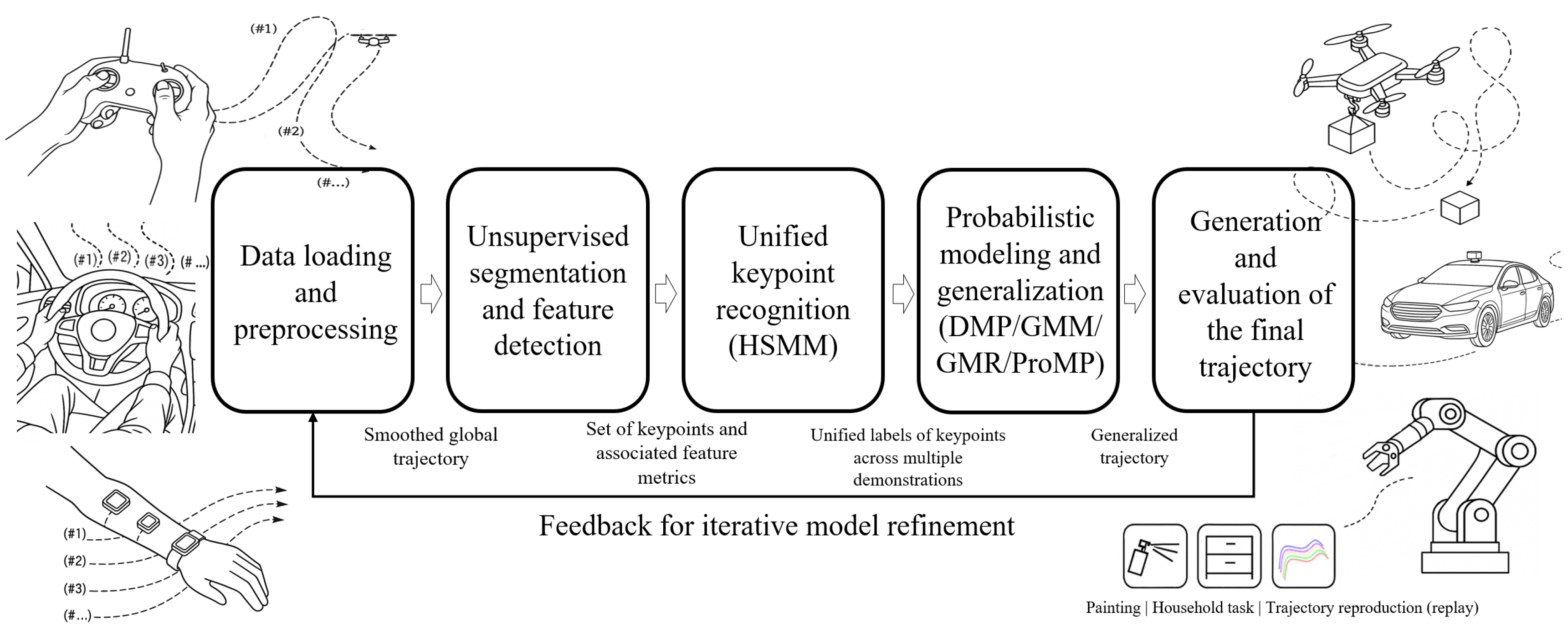
Figure 2.
Topological simplification and keyframe selection (persistence + NMS).
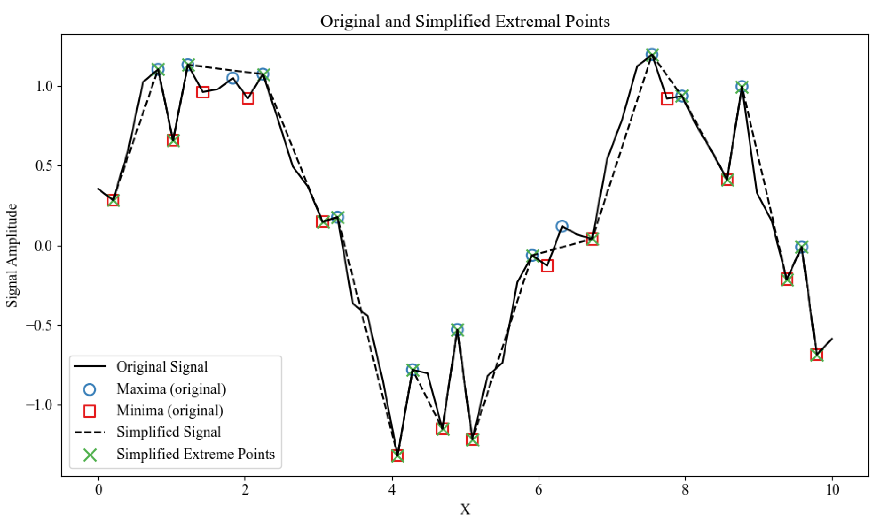
Figure 3.
Schematic of the HSMM. Circles denote random variables (top: observations; bottom: latent phases ). Solid arrows indicate Markovian dependencies; dashed links connect latent states to observation likelihoods. Shaded curves at the bottom depict state-specific duration distributions .
Figure 3.
Schematic of the HSMM. Circles denote random variables (top: observations; bottom: latent phases ). Solid arrows indicate Markovian dependencies; dashed links connect latent states to observation likelihoods. Shaded curves at the bottom depict state-specific duration distributions .
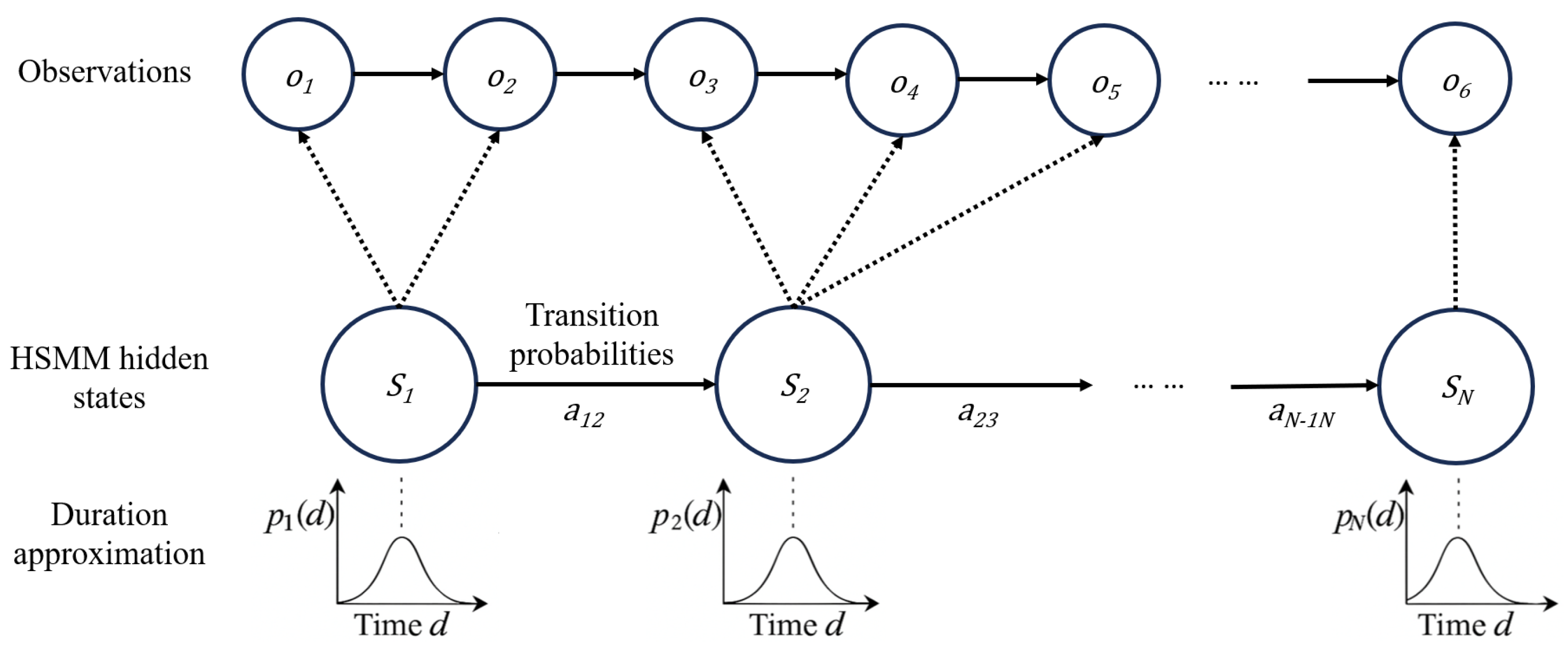
Figure 4.
Example 3D trajectories with keyframes (red dots) shown in three orthographic projections. Keyframes concentrate at motion-structure bends.
Figure 4.
Example 3D trajectories with keyframes (red dots) shown in three orthographic projections. Keyframes concentrate at motion-structure bends.
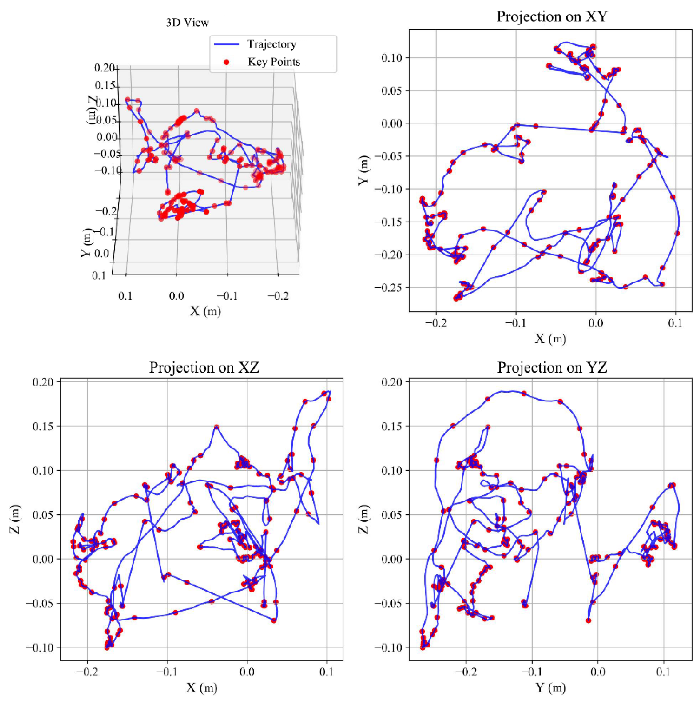
Figure 5.
Original trajectory (blue) versus HSMM reconstruction (red dashed). Boundaries align with salient kinematic transitions, validating the learned semantic phases.
Figure 5.
Original trajectory (blue) versus HSMM reconstruction (red dashed). Boundaries align with salient kinematic transitions, validating the learned semantic phases.
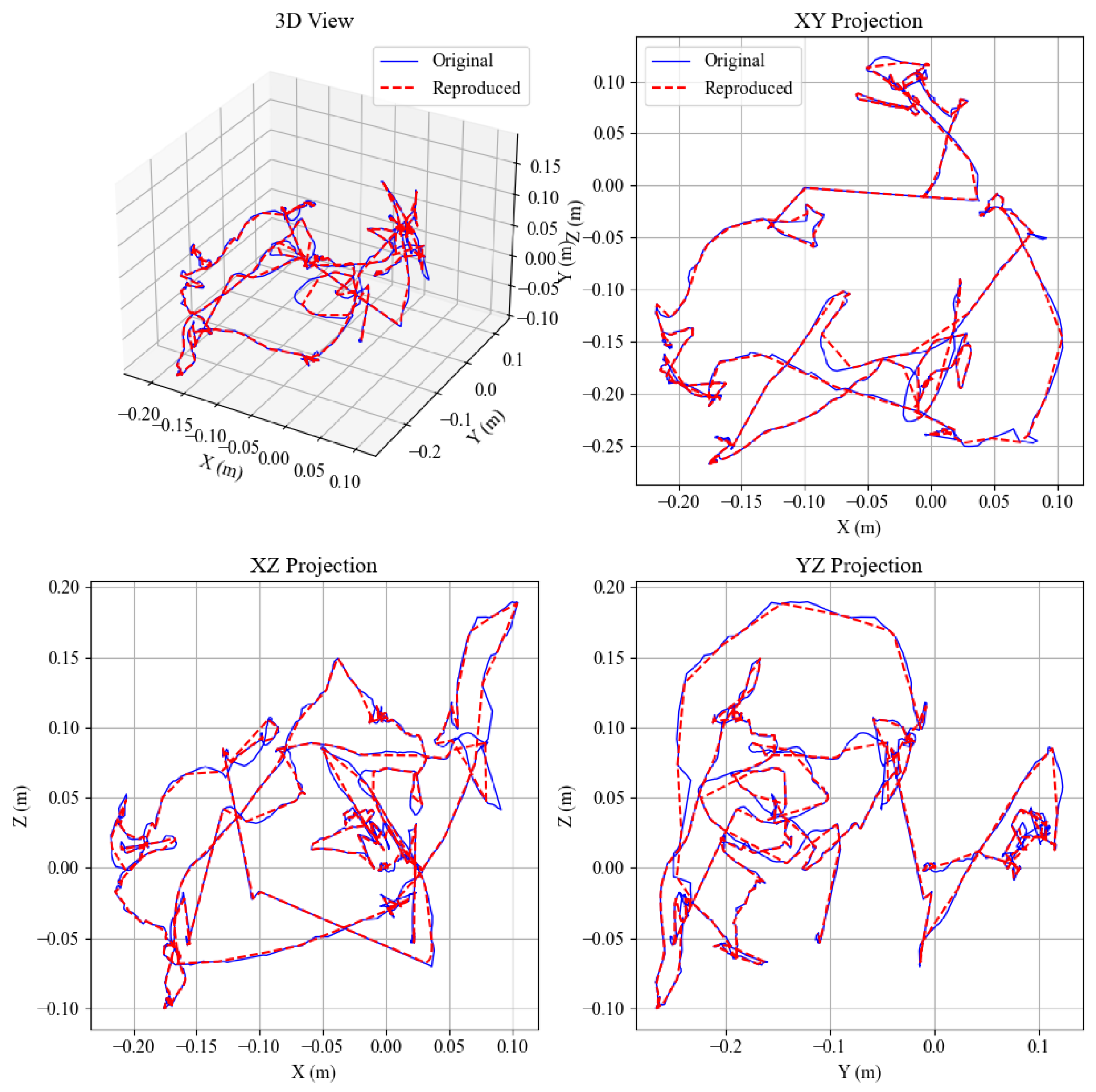
Figure 6.
HSMM-aligned ProMP generation. Blue curves show multiple aligned demonstrations; red curves depict ProMP samples under a new terminal constraint; translucent bands indicate the credible region. The two-level probabilistic structure (HSMM over phases; ProMP within segment) achieves global timing consistency with locally adjustable motion.
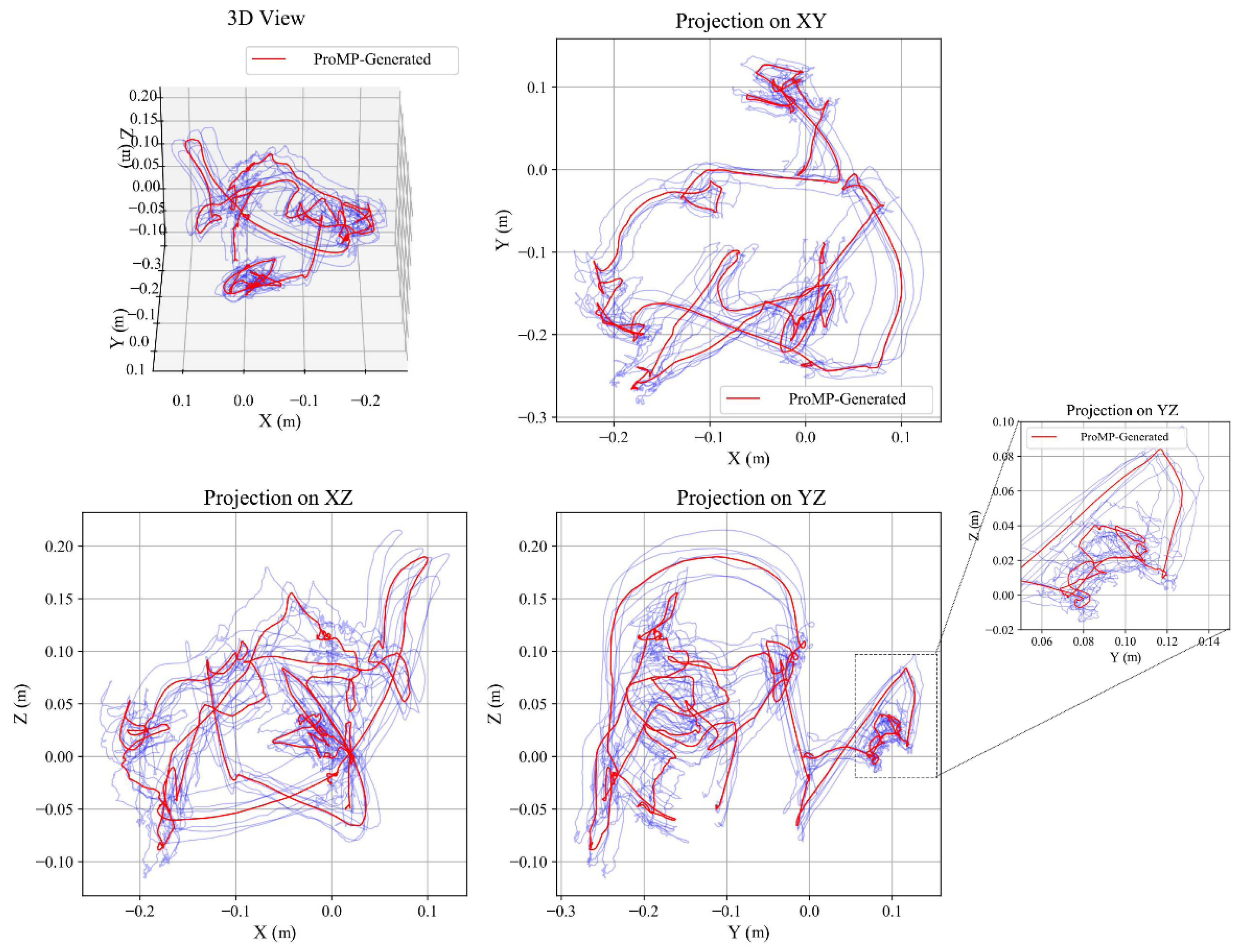
Figure 7.
UAV-Sim: environment and example demonstration trajectories.
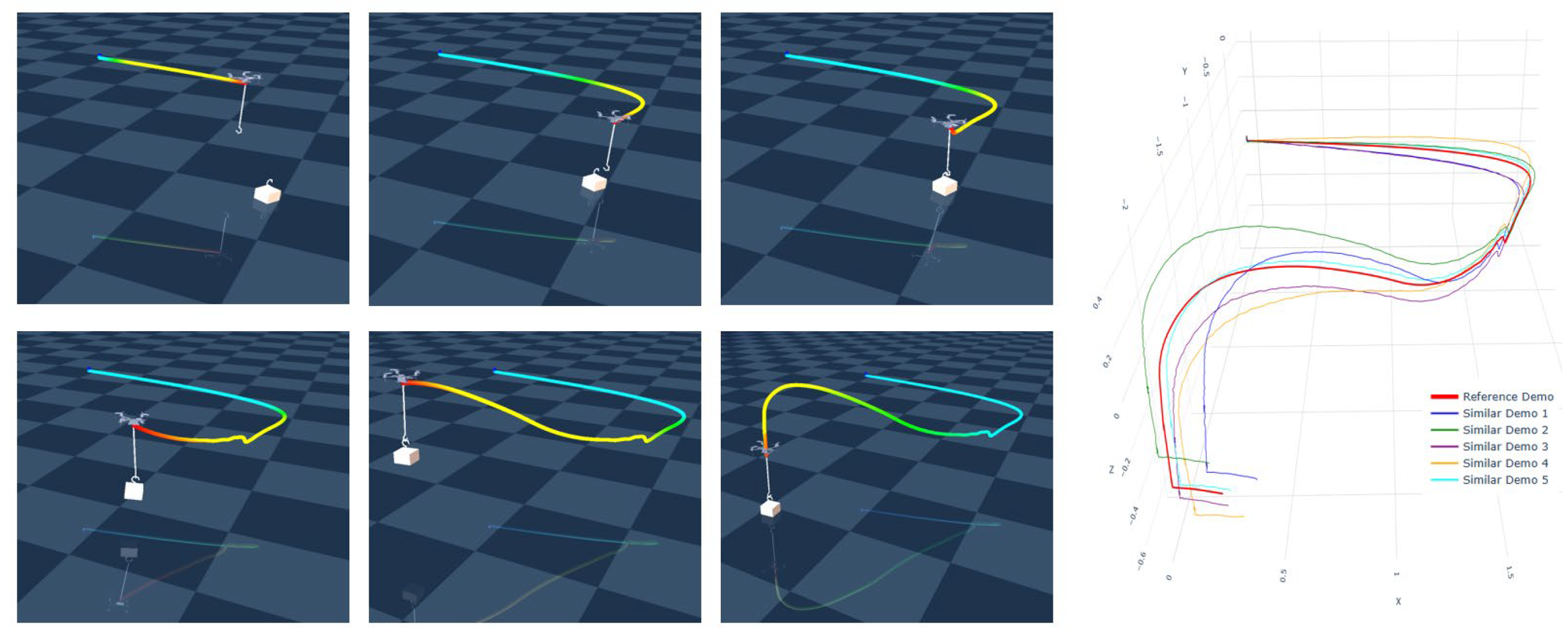
Figure 8.
AV-Sim (CARLA/MetaDrive): urban scenes and example demonstration trajectories.
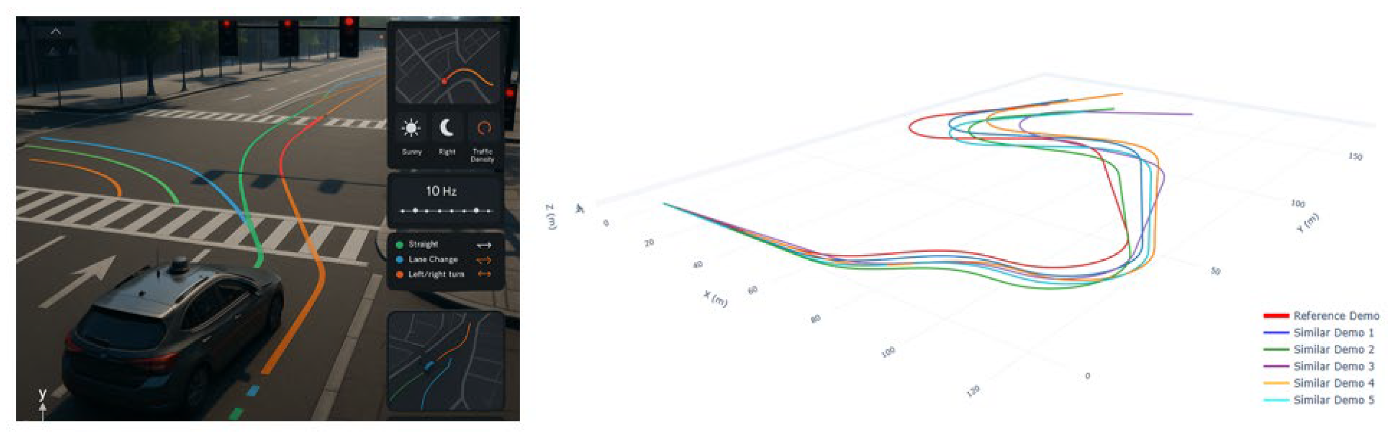
Figure 9.
Manip-Sim (robomimic/RLBench): assembly task (grasp–align–insert) and example trajectories.
Figure 9.
Manip-Sim (robomimic/RLBench): assembly task (grasp–align–insert) and example trajectories.
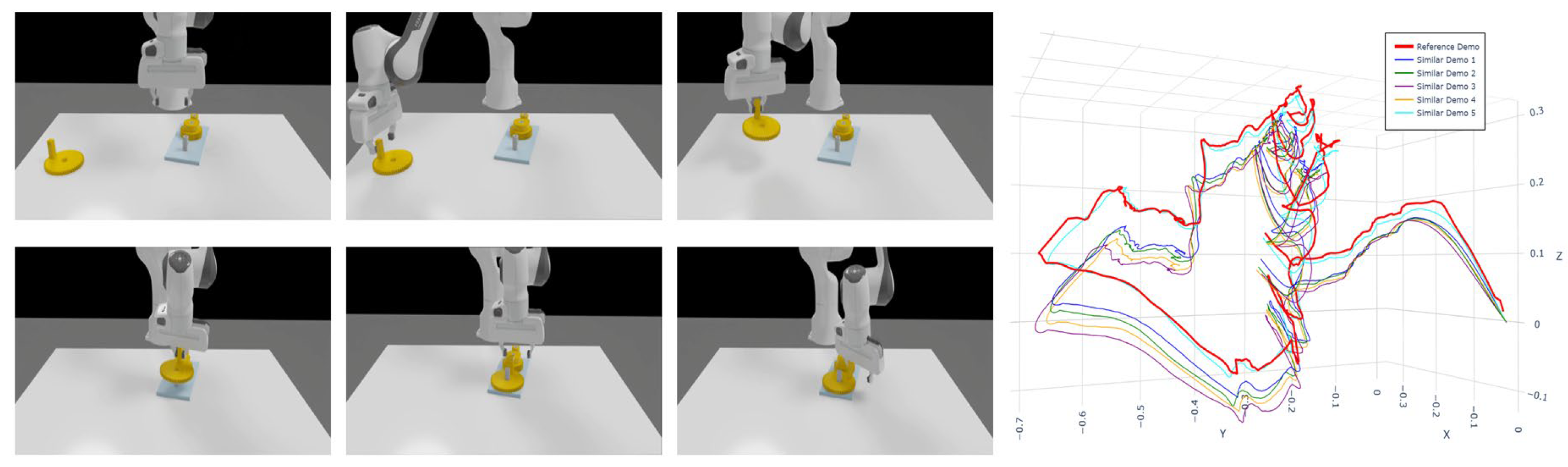
Figure 10.
Multi-demonstration overlay and feature time series. (a) 3-D overlays across demonstrations; (b) curvature, velocity, acceleration, direction-change rate, and fused saliency for one trajectory.
Figure 10.
Multi-demonstration overlay and feature time series. (a) 3-D overlays across demonstrations; (b) curvature, velocity, acceleration, direction-change rate, and fused saliency for one trajectory.
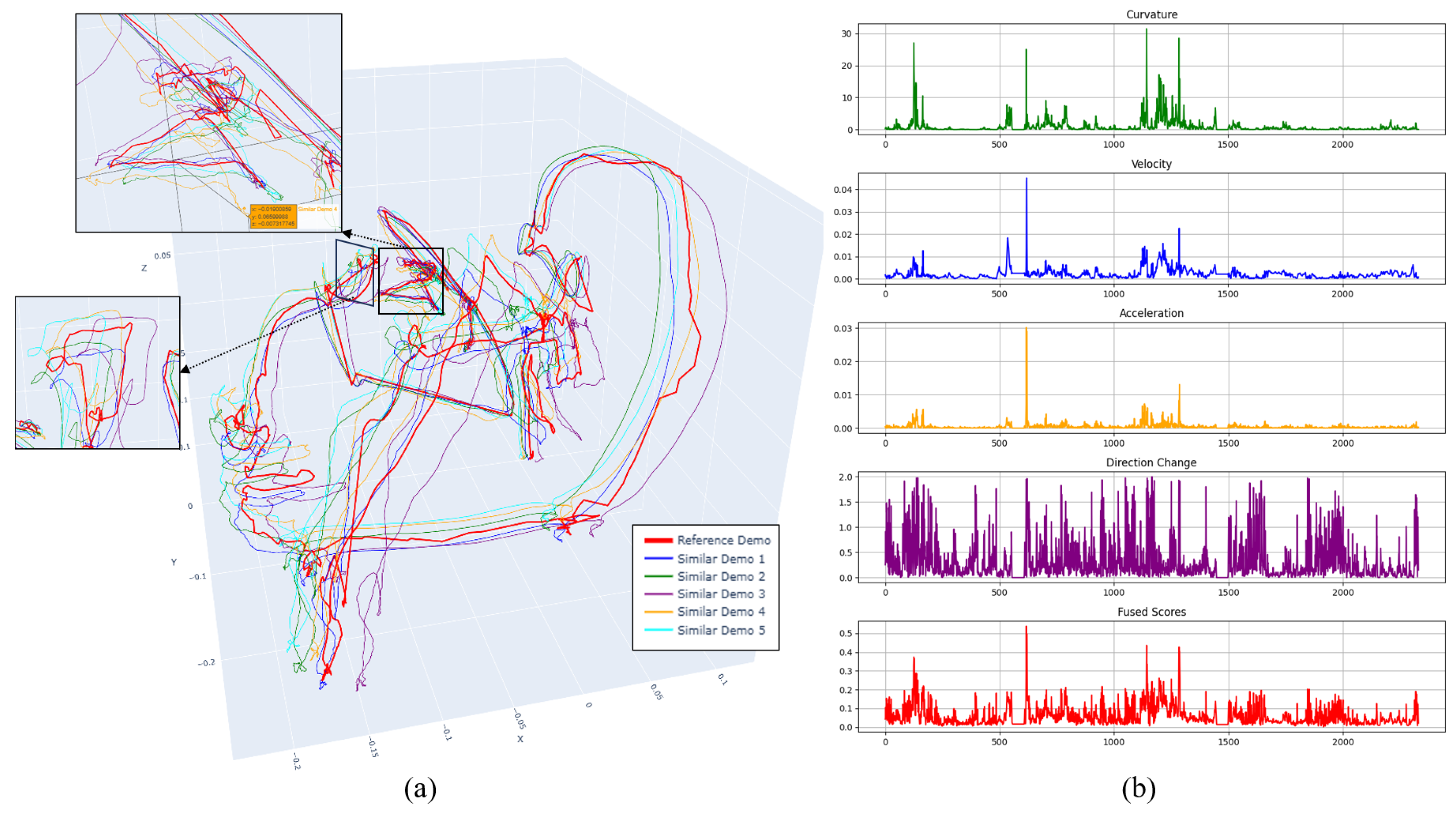
Figure 11.
Semantic time alignment with HSMM. (a) Before alignment: velocity vs. physical time; (b) After alignment: velocity vs. semantic time. Dashed lines show phase boundaries.
Figure 11.
Semantic time alignment with HSMM. (a) Before alignment: velocity vs. physical time; (b) After alignment: velocity vs. semantic time. Dashed lines show phase boundaries.
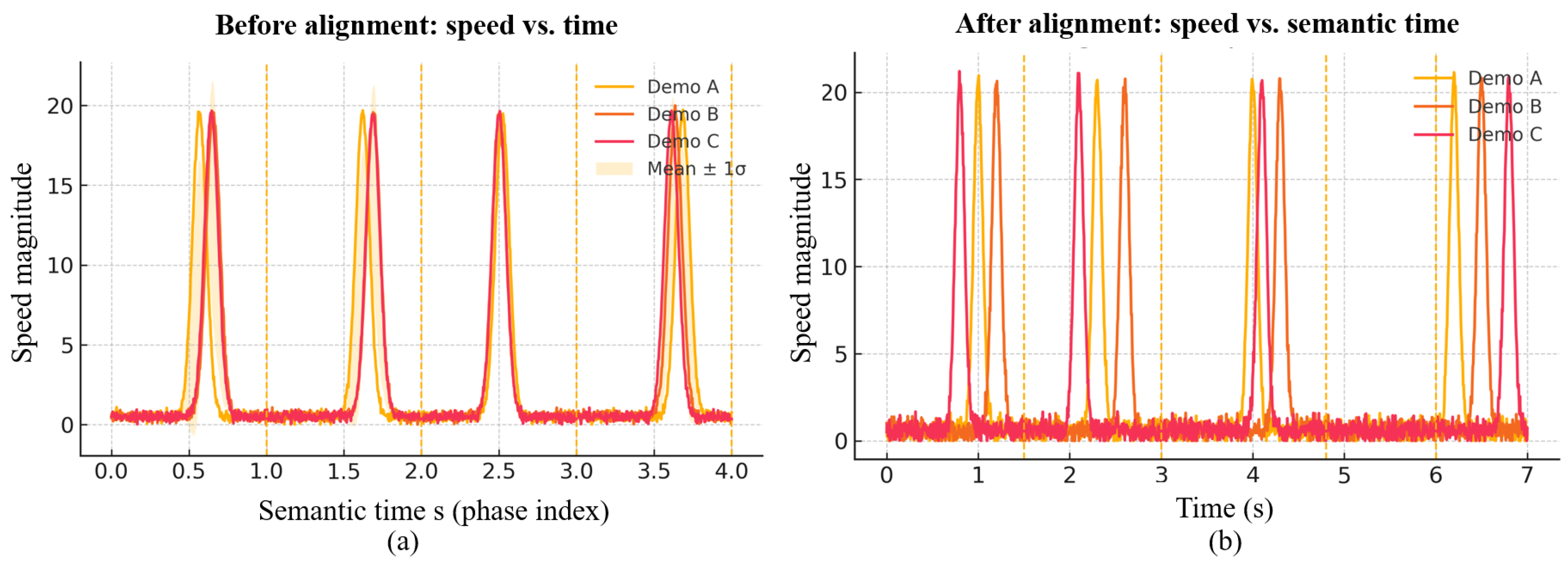
Figure 12.
Persistence threshold : effect on keyframe sparsity and reconstruction GRE (RMSE). Curves are means across subjects; shaded regions are BCa 95% CIs; vertical dashed line marks .
Figure 12.
Persistence threshold : effect on keyframe sparsity and reconstruction GRE (RMSE). Curves are means across subjects; shaded regions are BCa 95% CIs; vertical dashed line marks .
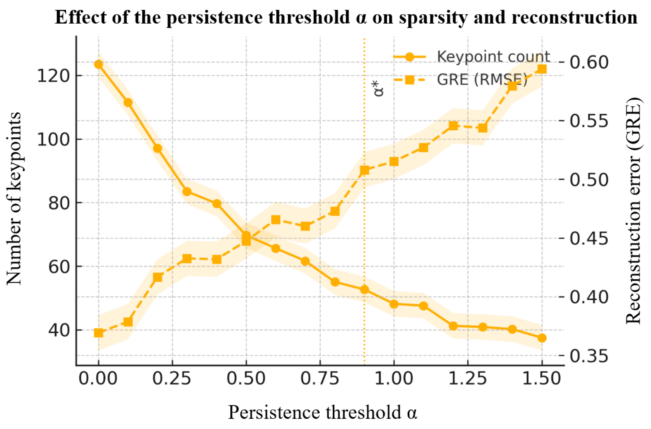
Figure 13.
HSMM state-number selection. Joint criterion of normalized AE and BIC; stars mark recommended per domain.
Figure 13.
HSMM state-number selection. Joint criterion of normalized AE and BIC; stars mark recommended per domain.
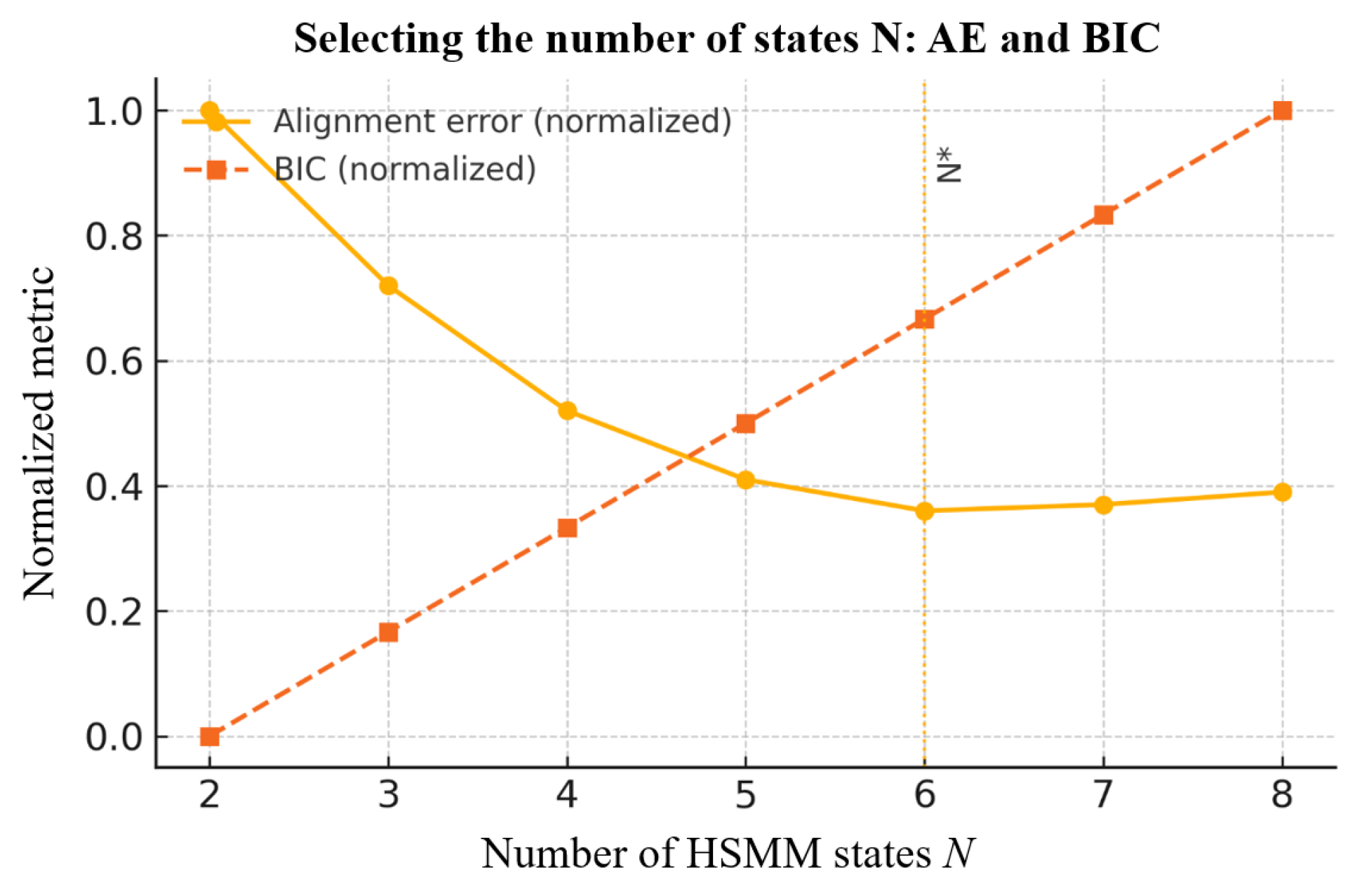
Figure 14.
In-segment generation comparison on a fixed semantic segment: linear interpolation, DMP, GMR, and ProMP.
Figure 14.
In-segment generation comparison on a fixed semantic segment: linear interpolation, DMP, GMR, and ProMP.
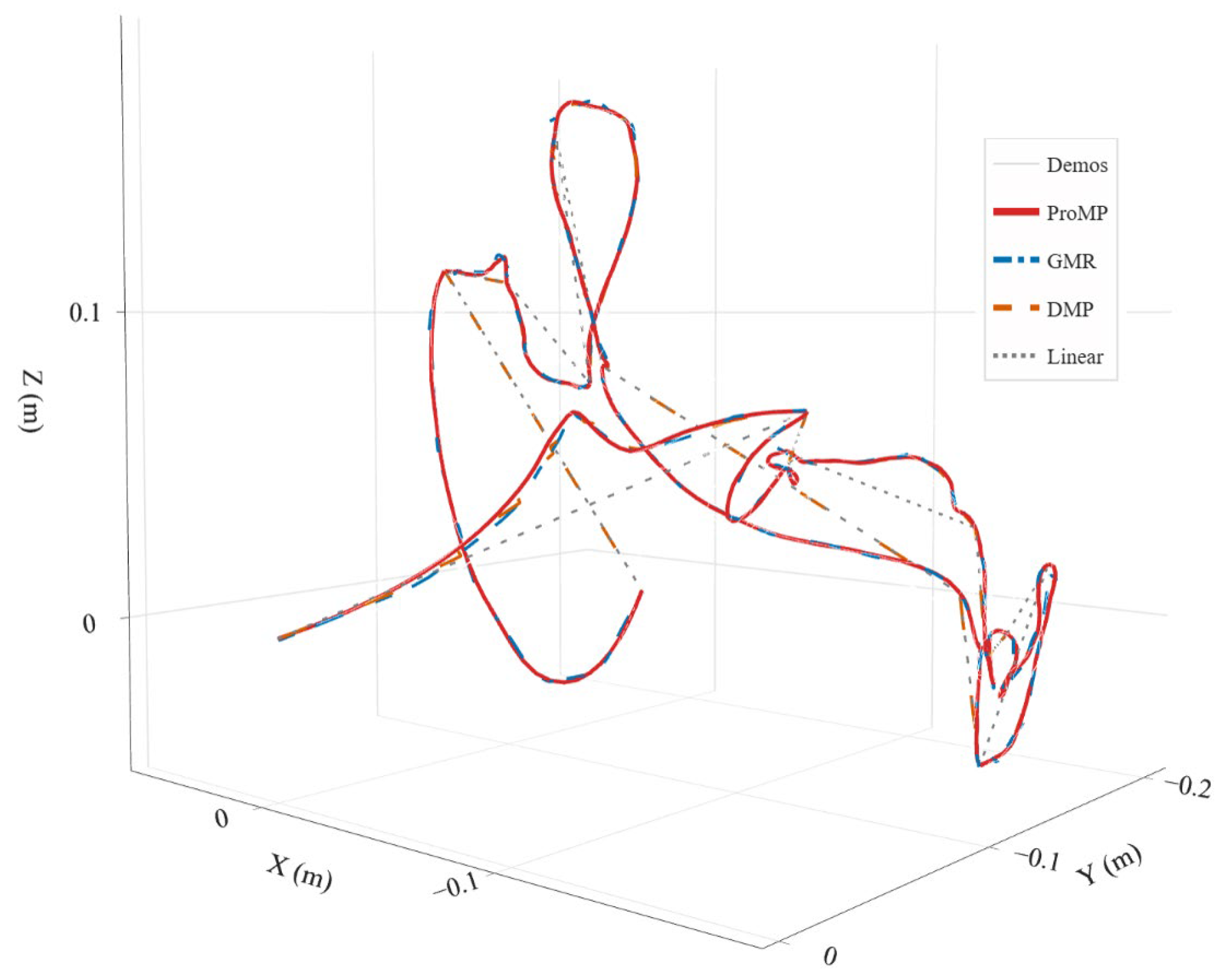
Table 1.
Segment-Level Motion Primitives: Properties and Trade-offs.
| Property | DMP | GMM/GMR | ProMP |
|---|---|---|---|
| Shape representation | Basis functions + 2nd-order stable system | Global Gaussian mixture over | Gaussian over weights w |
| Duration adaptation | Via time scaling | Requires resampling in phase | Basis-phase re-timing |
| Uncertainty | No closed-form (MC if needed) | Analytic | Analytic posterior over w |
| Online constraints | Endpoints/velocities easy | Refit or constrained regression | Exact linear-Gaussian conditioning |
| Execution smoothness | Low jerk (native dynamics) | Depends on mixture fit | Depends on basis and priors |
Table 2.
UAV-Sim (mean ± std; units: SOD/GRE in meters; “–“ = no probabilistic coverage).
| Method | SOD (m) | AE (s) | GRE (m) | TCR (%) | AAR (%) | Jerk | CR (%) |
|---|---|---|---|---|---|---|---|
| Curvature + quantile | 0.081 ± 0.019 | 0.55 ± 0.11 | 0.124 ± 0.027 | 34.9 ± 4.8 | 68.1 ± 6.0 | 1.22 ± 0.10 | – |
| Multi-feat (equal), no TDA/NMS | 0.071 ± 0.017 | 0.47 ± 0.10 | 0.110 ± 0.023 | 41.8 ± 5.1 | 73.8 ± 5.7 | 1.16 ± 0.08 | – |
| Multi-feat + TDA/NMS + HMM | 0.060 ± 0.014 | 0.41 ± 0.09 | 0.098 ± 0.019 | 54.6 ± 4.3 | 81.0 ± 4.8 | 1.08 ± 0.07 | – |
| BOCPD | 0.064 ± 0.016 | 0.46 ± 0.12 | 0.105 ± 0.022 | 51.0 ± 4.6 | 78.3 ± 5.4 | 1.14 ± 0.08 | – |
| Ours: +TDA/NMS+HSMM+ProMP | 0.045 ± 0.012 | 0.28 ± 0.07 | 0.082 ± 0.018 | 55.0 ± 4.0 | 88.7 ± 4.2 | 1.00 ± 0.06 | 94.9 ± 2.6 |
Table 5.
Ablation (relative % vs. full method; ↓/↑ indicates better/worse).
| Variant | ΔSOD | ΔAE | ΔGRE | ΔTCR | ΔAAR |
|---|---|---|---|---|---|
| No TDA (NMS only) | 12.30% | 9.60% | 6.70% | −9.4% | −5.8% |
| No NMS (TDA only) | 9.20% | 21.10% | 7.30% | −3.7% | −6.1% |
| Fixed equal weights (no ) | 18.60% | 14.40% | 9.10% | −1.1% | −7.7% |
| HMM in place of HSMM | 23.50% | 31.20% | 17.50% | ≈ 0 | −8.5% |
Table 6.
AE (s) under perturbations (AV-Sim).
| Perturbation | Setting | HMM (baseline) | HSMM (ours) | Δ |
|---|---|---|---|---|
| Time-warp | 0.61 | 0.39 | −36% | |
| Time-warp | 0.58 | 0.38 | −34% | |
| Gaussian noise | 0.57 | 0.4 | −30% | |
| Missing data | 20% random drop | 0.63 | 0.41 | −35% |
Disclaimer/Publisher’s Note: The statements, opinions and data contained in all publications are solely those of the individual author(s) and contributor(s) and not of MDPI and/or the editor(s). MDPI and/or the editor(s) disclaim responsibility for any injury to people or property resulting from any ideas, methods, instructions or products referred to in the content. |
© 2025 by the authors. Licensee MDPI, Basel, Switzerland. This article is an open access article distributed under the terms and conditions of the Creative Commons Attribution (CC BY) license (http://creativecommons.org/licenses/by/4.0/).
Copyright: This open access article is published under a Creative Commons CC BY 4.0 license, which permit the free download, distribution, and reuse, provided that the author and preprint are cited in any reuse.


