
Submitted:
20 August 2025
Posted:
22 August 2025
You are already at the latest version
Abstract
Analog and mixed-signal (AMS) integrated circuit (IC) design remains a critical yet challenging aspect within electronic design automation (EDA), primarily due to the inherent complexity, nonlinear behavior, and increasing variability associated with advanced semiconductor technologies. Traditional manual and intuition-driven methodologies for AMS circuit design, which rely heavily on iterative simulation loops and extensive designer experience, face significant limitations concerning efficiency, scalability, and reproducibility. Recently, machine learning (ML) techniques have emerged as powerful tools to address these challenges, offering significant enhancements in modeling, abstraction, optimization, and automation capabilities for AMS circuits. This review systematically examines recent advancements in ML-driven methodologies applied to analog circuit design, specifically focusing on modeling techniques such as Bayesian inference and neural-network-based surrogate models, optimization and sizing strategies, specification-driven predictive design, and AI-assisted design automation for layout generation. Through an extensive survey of existing literature, we analyze the effectiveness, strengths, and limitations of various ML approaches, identifying key trends and gaps within the current research landscape. Finally, the paper outlines potential future research directions aimed at advancing ML integration in analog IC design, emphasizing the need for improved explainability, data availability, methodological rigor, and end-to-end automation.
Keywords:
analog design
; mixed-signal design
; machine learning
; artificial intelligence
; modeling
; abstraction
; optimization
; sizing
; specification-driven
; assisted design
1. Introduction
AMS-ICs represent essential components widely utilized across numerous applications, including wireless communications, medical devices, automotive systems, biosensors, and security electronics. Unlike digital circuits, AMS circuits often involve intricate and nonlinear interactions, making their design particularly challenging [1]. With the continuous scaling of semiconductor technologies, the complexity and variability of these circuits have increased significantly, imposing additional difficulties on designers and EDA tools [1,2].
Traditionally, AMS circuit design has relied heavily on expert intuition and manual tuning, where designers iteratively adjust transistor sizes, bias currents, and passive components to meet targeted performance specifications. This manual approach becomes increasingly inefficient and unreliable in advanced technology nodes due to severe process variations and complex physical phenomena [1]. Furthermore, the iterative design process contributes significantly to lengthy development cycles and increased time-to-market pressures [2].
In contrast, digital circuit design has greatly benefited from extensive automation and established EDA tools, significantly reducing design time and improving predictability and reproducibility. Unfortunately, the AMS design process has not experienced comparable levels of automation, partly due to the inherent complexity of analog design and the lack of effective modeling methods and tools capable of handling nonlinear circuit behavior [2,3].
In recent years, ML techniques have emerged as promising candidates to bridge this gap by providing computationally efficient methods for modeling, optimization, and design automation of AMS circuits. ML methods, including artificial neural networks (ANNs), Bayesian models, reinforcement learning (RL), and Support Vector Machines (SVMs), have demonstrated notable success in capturing nonlinear relationships, managing high-dimensional variability, and enhancing the predictability of circuit performance [1,4]. Specifically, ML-driven approaches facilitate significant acceleration in analog circuit design by reducing the reliance on computationally expensive simulations and enabling the reuse of knowledge across design tasks and contexts [3,5].
This review paper systematically explores state-of-the-art ML techniques and methodologies applied to AMS-IC design. Section 2 presents an overview of ML fundamentals, introducing key paradigms such as supervised, semi-supervised, unsupervised, and RL, learning tasks and describing the primary models associated with each category. Section 3 reviews relevant literature and covers topics including circuit modeling and abstraction, optimization and sizing techniques, specification-driven design, and AI-assisted design automation methods. Section 4 provides discussions and conclusions drawn from the surveyed works, while Section 5 highlights potential directions for future research in the field.
In conclusion, we highlight critical insights derived from the analysis, identify existing research gaps, and propose future directions for advancing the integration of ML in analog IC design automation. Through this comprehensive review, we aim to illustrate how ML can substantially improve analog circuit design processes, reduce time-to-market, and enhance overall design productivity and innovation in the semiconductor industry.
2. ML an Overview
2.1. Terminology and Learning Paradigms
ML refers to computational algorithms and statistical techniques that enable computer systems to recognize patterns, learn from data, and make informed decisions without explicit programming [6,7]. Fundamental terms include features, representing variables describing the input data; labels, the output variables or targets; training sets for model building; validation sets for parameter tuning; and test sets for performance evaluation [7].
ML paradigms encompass supervised, semi-supervised, unsupervised, and RL, each characterized by unique methodologies and objectives [8,9]. These paradigms differ primarily in the availability of labeled data and the learning objective and play a central role in determining the choice of algorithms and models used in AMS-IC design.
2.2. Supervised, Semi-Supervised, Unsupervised, and RL Tasks
ML tasks are generally categorized based on the availability of labeled data and the nature of the learning objective. Understanding these categories is essential for selecting appropriate models and methodologies in AMS-IC design. The four primary learning paradigms are supervised, semi-supervised, unsupervised, and RL—each with distinct characteristics and applications.
2.2.1. Supervised Learning
Supervised learning is a fundamental paradigm in ML where a model is trained on a dataset comprising input–output pairs (). The objective is to learn a function that maps input vectors to target outputs , by minimizing the discrepancy between the predicted and true values [10,11]. The relationship between the input and output is typically modeled as:
where denotes the input feature vector, is the corresponding output (dependent variable), represents the predictive model parameterized by , is an error term accounting for noise or model imperfections.
The model parameters are learned by minimizing a predefined loss function , such as the mean squared error (MSE) for regression tasks or the cross-entropy loss for classification problems. The optimization objective over a labeled dataset is formulated as:
where denotes the number of labeled training examples. The choice of the loss function depends on the specific task and data characteristics [9,11].
2.2.2. Semi-Supervised Learning
Semi-supervised learning (SSL) is a learning paradigm that combines a small amount of labeled data with a large volume of unlabeled data to improve generalization [12,13]. By leveraging the structure inherent in the unlabeled data, SSL techniques can enhance model performance, particularly when labeled samples are scarce or costly to obtain [14].
Let the dataset be partitioned into a labeled subset and an unlabeled subset , such that:
where: denotes the labeled data, denotes the unlabeled data.
The goal is to learn a function that generalizes well across both subsets. The typical training objective in semi-supervised learning is formulated as:
where: is the supervised loss applied to labeled data, cross-entropy or MSE, is an unsupervised loss that regularizes the model using unlabeled data (e.g., consistency loss, entropy minimization, or pseudo-labeling) and is a weighting parameter that controls the influence of the unlabeled loss [13,15].
This formulation allows the model to benefit from the abundance of unlabeled data by guiding its predictions to be consistent and confident, even when explicit supervision is limited. SSL has gained increasing traction in domains where labeling is expensive, or domain expertise is required—making it particularly suitable for AMS-IC design workflows involving large unlabeled simulation datasets [1].
2.2.3. Unsupervised Learning
Unsupervised learning refers to a class of ML techniques that aim to discover underlying patterns, structures, or latent representations from data without the use of labeled outputs [16]. This paradigm is particularly valuable when labeled data is scarce or unavailable, and is commonly used in tasks such as clustering, dimensionality reduction, density estimation, and anomaly detection [17].
Formally, given a dataset of input samples , the objective is to transform or group these inputs into a latent representation , such that:
where: , denotes the observed input data, , represents the learned latent variables, cluster indices, or lower-dimensional embeddings [11].
Two widely used unsupervised learning techniques include clustering like, K-Means and dimensionality reduction like, Principal Component Analysis (PCA).
K-Means clustering partitions a dataset into clusters by minimizing the within-cluster sum of squared distances. The optimization problem is given by:
where: is the -th data point, is the centroid of cluster and is the total number of data points [17].
PCA is a linear dimensionality reduction technique that finds the directions of maximum variance in the data. It seeks to project the input data onto a lower-dimensional subspace while retaining the most informative components. The optimization objective is:
where: is the projection matrix (), is the variance of the projected data and the constraint ensures that the projection vectors are orthonormal [18].
2.2.4. RL
RL is a computational learning paradigm in which an agent interacts with an environment in a sequential decision-making process to learn an optimal policy. The agent receives feedback in the form of scalar rewards and aims to maximize the long-term cumulative reward [19,20]. This framework is typically modeled as a Markov Decision Process (MDP). An MDP is formally defined as a 5-tuple:
where: is the set of all possible states, is the set of all possible actions is the transition probability function defining the probability of transitioning to state given the current state s and action , is the reward function specifying the immediate reward received after taking action in state and is the discount factor, which balances the importance of immediate versus future rewards [20].
The goal of the agent is to learn a policy , which defines the probability of taking action in state , such that the expected return is maximized:
To evaluate the quality of a policy, the state-value function is defined as the expected return when starting from state and following policy thereafter:
The state-value function satisfies the Bellman equation, which expresses a recursive relationship:
This recursive formulation forms the basis for various dynamic programming and RL algorithms, such as value iteration, policy iteration, and Q-learning [21,22].
RL techniques are increasingly adopted in AMS-IC design to enable closed-loop optimization, autonomous tuning, and exploration of design spaces where explicit modeling is complex or infeasible[5].
2.3. Learning Models
ML offers a diverse set of models suited to a range of data-driven tasks, from regression and classification to optimization and surrogate modeling. While many models exist—such as decision trees, ensemble methods, and probabilistic graphical models—certain families have proven especially effective in the context of AMS-IC design. This section focuses on three of the most widely adopted models in the AMS-IC literature: Bayesian models, SVMs, and ANNs. These models have demonstrated strong performance in tasks such as circuit modeling, performance prediction, optimization, and design automation. For completeness, foundational models like linear and logistic regression are also briefly discussed, as they serve as important baselines and are occasionally used in early-stage design exploration.
2.3.1. Bayesian Models
Bayesian models are probabilistic frameworks that incorporate prior knowledge and update beliefs using observed data. They are particularly well-suited for AMS-IC design tasks where uncertainty quantification is critical, such as performance prediction under process variation or surrogate modeling [23,24].
Bayes’ theorem provides the basis:
where: is the posterior probability of parameters given data , is the likelihood of the data under model parameters, is the prior belief about parameters and presents the marginal likelihood, normalization factor.
Bayesian models play a critical role in AMS-IC design. They are employed in surrogate modeling to efficiently approximate circuit performance metrics, enabling rapid and cost-effective design space exploration. Bayesian optimization (BO) facilitates automated sizing and tuning of circuit parameters, offering a data-efficient strategy for navigating complex design landscapes [25].
Furthermore, Bayesian approaches to uncertainty modeling help quantify and mitigate the effects of post-layout variations, thereby improving the robustness and predictability of circuit performance. Figure 1 provides a general overview of the Bayesian inference process, showing how prior beliefs are updated with observed data to form the posterior distribution.
2.3.2. ANNs
ANNs are a class of ML models inspired by the structure and functioning of the human brain. They consist of layers of interconnected nodes—commonly referred to as neurons—that can approximate complex nonlinear relationships between inputs and outputs [10]. Among various architectures, the feedforward neural network (FNN) is most widely adopted in AMS-IC design due to its simplicity and effectiveness in function approximation tasks. Figure 2 presents a general structure of a feedforward ANN with fully connected layers.
The activation of a neuron in a feedforward layer is computed as:
where: denotes the output of neuron , represents the input feature, is the weight connecting input to neuron , is the bias term associated with neuron is a nonlinear activation function, such as the sigmoid, hyperbolic tangent (tanh), or rectified linear unit (ReLU) [7].
By stacking multiple layers of such neurons, ANNs are capable of learning highly expressive mappings between high-dimensional input and output spaces. The parameters and are typically learned via backpropagation using gradient-based optimization.
In AMS-IC design, ANNs are increasingly utilized due to their flexibility and ability to learn from large, noisy datasets. Key applications include specification-to-parameter mapping, where direct relationships are learned between high-level performance targets and transistor-level design parameters; layout generation and performance prediction, which involve estimating post-layout metrics from pre-layout features or assisting in layout synthesis; and post-layout regression modeling, which captures complex, nonlinear relationships between layout-induced parasitics and circuit-level performance. These capabilities make ANNs valuable tools for surrogate modeling, design space exploration, and layout-aware performance estimation within modern AMS-IC design flows.
2.3.3. SVMs
SVMs are supervised learning models widely used for both classification and regression tasks. They are particularly valued for their ability to construct robust decision boundaries by maximizing the margin between classes, thus enhancing generalization performance [26,27]. Figure 3 shows a SVM classification example with decision boundary and margin visualization.
In the case of linearly separable data, SVMs aim to find the hyperplane that best divides the data into distinct classes with the greatest possible margin. The decision function for a linear SVM is given by:
subject to the constraint:
where: is the input feature vector, is the class label associated with , is the weight vector defining the orientation of the hyperplane, and is the bias term defining the offset [27].
For nonlinearly separable datasets, SVMs employ kernel functions to implicitly map the input data into a higher-dimensional feature space where linear separation becomes feasible. Common kernel choices include the Radial Basis Function (RBF), polynomial, and sigmoid kernels [26].
2.3.4. Linear and Logistic Regression
Linear and logistic regression are foundational statistical learning methods that serve as interpretable and computationally efficient tools in many ML tasks. In the context of AMS integrated circuit design, these models are commonly used for rapid performance estimation, classification, and as baseline models for benchmarking more complex approaches.
2.3.4.1. Linear Regression
Linear regression predicts a continuous outcome by modeling a linear relationship between input features and the target variable [28]. The predictive model is given by:
where: is the predicted response, are the input features, is the intercept term, and are the model coefficients learned from data (Figure 4).
This method is most suitable when the underlying relationship between input and output is approximately linear and serves as a useful baseline in regression problems within AMS design.
2.3.4.2. Logistic Regression
Logistic regression is used for binary classification problems, modeling the probability that a given input belongs to a particular class [29]. The model uses the logistic (sigmoid) function to map real-valued inputs to a probability in the range [0,1]:
where denotes the binary class label and the parameters are learned from data through maximum likelihood estimation [28,29] (Figure 5).
In AMS-IC design, linear and logistic regression models remain valuable tools due to their simplicity, transparency, and low computational cost. They are particularly effective in performance region classification, helping to identify whether circuits meet acceptable performance thresholds. These models are also useful in early-stage design modeling, where they provide fast and interpretable rule-based approximations in scenarios with limited data or low design complexity. Additionally, they serve an important role in benchmarking, offering a baseline for evaluating the performance gains achieved by more advanced models such as ANNs or ensemble methods, especially in contexts where interpretability and efficiency are critical.
2.3.5. Decision Trees
Decision trees (DT) are non-parametric ML models used for both regression and classification tasks. They operate by recursively partitioning the input space into distinct regions based on feature thresholds [30,31]. Each internal node in the tree corresponds to a decision rule on a feature, and each leaf node represents a prediction—either a class label (in classification) or a numeric value (in regression). Due to their interpretability and simplicity, DTs are particularly appealing for early-stage modeling and rule extraction in AMS-IC design.
For regression tasks, the decision tree aims to minimize the variance of outputs within each region. The training objective can be defined as:
where: denotes the terminal region (leaf node) defined by the tree structure, is the mean of the target values for all , and is the total number of leaves (regions).
The model selects features and split points greedily, based on impurity reduction measures such as Gini impurity, entropy, for classification, or variance reduction, for regression [31] (Figure 6).
In AMS-IC design, DTs are employed for a range of tasks due to their interpretability and adaptability. They are used in lightweight regression modeling to quickly approximate circuit behavior from limited datasets, and in performance estimation under constraints by capturing simple, rule-based relationships between design variables and performance metrics [1,32]. Moreover, DTs serve as base learners in ensemble methods such as Random Forests and Gradient Boosted Trees, significantly enhancing prediction accuracy and robustness. Although individual DTs can be prone to overfitting, their integration into ensemble frameworks makes them a versatile and powerful component of ML workflows in AMS-IC design.
2.4. Evaluation Metrics
Evaluating the performance of ML models is essential for ensuring their reliability and suitability in design tasks. Depending on the learning objective—classification or regression—different metrics are used to assess model accuracy, robustness, and explanatory power [33].
2.4.1. Classification Metrics
For classification problems, performance is typically assessed using a set of metrics derived from the confusion matrix, which categorizes prediction outcomes into four groups: True Positives (TP), representing correctly predicted positive instances; True Negatives (TN), correctly predicted negative instances; False Positives (FP), negative instances incorrectly predicted as positive; and False Negatives (FN), positive instances incorrectly predicted as negative [34]. Based on these values, the core evaluation metrics are defined as follows:
Precision is particularly important in scenarios where false positives carry significant consequences—for example, incorrectly flagging valid circuit designs as invalid, which may lead to unnecessary design rework or discarded solutions. Recall becomes critical when false negatives are costly, such as missing potentially valid design candidates that meet performance requirements. The F1-score provides a balanced measure of precision and recall, making it especially valuable in cases of class imbalance, where relying solely on accuracy may be misleading. This balance ensures that both types of misclassification are considered when evaluating model performance.
2.4.2. Regression Metrics
For regression tasks, performance is typically evaluated using error-based metrics that quantify the difference between predicted and actual values [35]. MSE measures the average of the squares of the errors, emphasizing larger errors more due to squaring, which makes it sensitive to outliers. Mean absolute error (MAE) calculates the average of the absolute differences between predicted and actual values, offering a more interpretable measure of average error and being less affected by outliers [36]. The Coefficient of determination (R²) represents the proportion of variance in the dependent variable that can be explained by the independent variables; an R² value of 1 indicates perfect prediction, while a value of 0 means the model fails to capture any variability in the data [35,37]. These metrics together provide a comprehensive view of model accuracy and reliability in regression settings.
where: consists of the observed values, represents the predicted values, is the mean of observed values, and is the number of observations.
3. Review for Analog Design Based on ML Methods
3.1. Studies Categorization
This review includes a total of thirty-four articles, comprising twenty-nine conference papers and five journal articles (Figure 7), spanning the period from 2012 to 2024 (Figure 8). The studies are organized into four main thematic categories: Modeling & Abstraction of Analog Circuits, Optimization & Sizing Techniques, Specification-Driven Design, and AI-Assisted Design Automation.
Specifically, the Modeling & Abstraction of Analog Circuits category includes thirteen studies, two journal articles and eleven conference papers. The Optimization & Sizing Techniques section comprises ten articles, with three published in journals and seven in conferences. The Specification-Driven Design category includes seven conference papers, while the AI-Assisted Design Automation category consists of four conference publications (Figure 9).
3.2. Modeling & Abstraction of Analog Circuits
The complexity and nonlinearity inherent in analog ICs pose substantial challenges for efficient design, simulation, and verification. Traditional circuit modeling approaches, while accurate, are often computationally intensive and lack the flexibility to scale across diverse topologies or performance regimes. In recent years, ML techniques have emerged as powerful tools for abstracting analog circuit behavior, enabling faster simulation, improved performance prediction, and enhanced design reuse. Within this context, modeling methods based on ANNs, Gaussian processes, and Bayesian learning have demonstrated the ability to capture nonlinear circuit dynamics, learn from limited data, and generalize across design spaces. The works reviewed in this section employ these AI-driven models to create surrogate abstractions of analog blocks, ranging from op-amps to mixed-signal components, significantly accelerating simulation workflows and supporting early-stage design decisions. This section outlines the main modeling strategies, abstraction levels, and application domains addressed in recent literature.
A Bayesian model fusion (BMF) technique for improving the efficiency of parametric yield estimation in AMS circuits was introduced in [38]. The method utilizes simulation data from early design stages—such as schematic-level analysis—to construct informative priors for estimating complex post-layout performance distributions. A small number of late-stage simulations are then used in conjunction with maximum-a-posteriori (MAP) inference within a Bayesian framework to estimate yield. The approach was evaluated on ring oscillator (RO) and static random-access memory (SRAM) read path circuits, demonstrating up to a 3.75× speed-up in simulation runtime over traditional kernel-based techniques, while maintaining high predictive accuracy. In [39], the authors introduced Co-Learning BMF (CL-BMF), an advanced performance modeling technique for AMS circuits. CL-BMF combines coefficient side information (CSI) with performance side information (PSI) within a Bayesian inference framework represented as a graphical model. The key innovation lies in leveraging a low-complexity model—based on inexpensive performance metrics—to generate pseudo samples that facilitate the training of a high-complexity model using fewer costly simulations. Case studies on a RO and a 60 GHz low-noise amplifier (LNA) fabricated in 32nm Silicon on insulator (SOI) complementary metal oxide semiconductor (CMOS) demonstrate that CL-BMF achieves up to a 5× reduction in modeling cost while preserving high accuracy. The same group [40] proposed BMF, a technique for efficient performance modeling of AMS circuits. The method leverages early-stage simulation data as prior knowledge to support post-layout performance prediction, thereby reducing the number of late-stage simulations required. BMF models performance correlations between design stages using Bayesian inference, employing both zero-mean and nonzero-mean priors combined with MAP estimation. This allows the construction of accurate post-layout models, even in high-dimensional variation spaces. Experimental validation on a RO and an SRAM read path circuit fabricated in a 32nm CMOS SOI process demonstrates up to a 9× speed-up in runtime, along with improved accuracy over sparse regression methods. In [41], the authors proposed a compositional neural-network (CompNN) approach for modeling complex analog circuits as multiple input-multiple output (MIMO) systems. They utilized individual nonlinear autoregressive exogenous (NARX) networks to model specific input-output relationships like, trimming, load jump, and line jump of a band-gap voltage reference (BGR) circuit. These outputs are then composed using a time delay neural network (TDNN) to replicate the system behavior efficiently. The proposed model provides over 17× speedup in transient simulation compared to transistor-level models while preserving accuracy. In [42], the authors introduced a hierarchical performance modeling methodology leveraging Bayesian Co-learning (BCL). The approach decomposes the IC into hierarchical blocks and utilizes a combination of low-cost labeled and abundant unlabeled data to build accurate performance prediction models. Within this framework, they constructed a Bayesian model that integrates prior coefficient information, low-dimensional block-level models, and high-dimensional circuit-level models via semi-supervised learning. To reduce simulation cost, the method generates pseudo-labeled data from the low-level models. Experimental results on automatic delay compensation (ADC) delay-line and multi-stage amplifier circuits demonstrate notable runtime savings—up to 3.66×—without compromising model accuracy. In [43], the authors proposed a self-adaptive multiple starting point (Smart-MSP) optimization approach for analog circuit synthesis. The approach integrates heuristic-biased starting point selection, sparse regression–based surrogate modeling, and probabilistic TABU (P-TABU) strategies to reduce simulation overhead. These mechanisms enable the optimizer to learn from past local searches and adaptively focus on high-potential regions within the design space. When compared to conventional optimization algorithms such as genetic algorithm (GA), simulated annealing (SA), particle swarm optimization (PSO), differential evolution (DE), and clustered simulated forced oscillation. Smart-MSP achieves a 2.6× to 12.5× speed-up while maintaining or improving solution quality. A parallelized implementation further enhances performance on large-scale synthesis tasks. Gao [44] proposed a Bayesian neural network (BNN)-based method for modeling performance trade-offs in analog circuit design. The authors propose using a single BNN, trained via automatic differential variational inference (ADVI), to simultaneously model multiple performance indicators of a circuit. This BNN is integrated into a BO framework that iteratively refines Pareto front approximations using a modified multi-objective evolutionary algorithm based on decomposition (MOEA/D) evolutionary algorithm. Compared to traditional surrogate models such as Gaussian processes, the BNN approach more effectively captures correlations among points of interests (PoIs), thereby enhancing modeling efficiency and accuracy. Experimental results on charge pump and low-power amplifier circuits demonstrate a 2× reduction in required simulations compared to prior methods. A hybrid analog IC synthesis method was proposed in [45], incorporating ANNs into a simulation-driven optimization flow guided by the SPEA2 evolutionary algorithm. Instead of discarding simulation data after each generation, the method reuses it to incrementally train ANNs as performance estimators. Once sufficiently trained, these networks partially replace the simulator, significantly reducing execution time. The approach was validated on a single-stage amplifier and a folded cascode operational transconductance amplifier (OTA), resulting in up to a 64.8% speed-up without degrading optimization performance. In [46] a Berkeley analog generator network (BagNet) was introduced as a layout-aware analog circuit optimization framework that integrates evolutionary algorithms with a deep neural network (DNN) based oracle. The system utilizes the Berkeley analog generator (BAG) to create manufacturable layouts, while a DNN discriminator mimics simulation behavior, enabling selective evaluation of promising designs. By combining layout generation, simulation feedback, and ML–guided selection, BagNet achieved a reported 20× to 300× speed-up in post-layout optimization across a range of analog - radio frequency circuits (RFCs), including operational amplifiers and optical receivers. A neural network (NN) based Gaussian process regression (GPR) approach for BO was proposed in [47]. Unlike traditional GPR methods that rely on predefined kernels, this hybrid model uses a NN to learn feature embeddings that implicitly define the GP kernel. The resulting GP-NN model is paired with a weighted expected improvement (WEI) acquisition function and enhanced through ensemble learning to improve uncertainty estimation. The approach demonstrated reduced simulation counts and computational cost in large design spaces, with successful application to operational amplifier and charge pump circuits. A sparse performance modeling approach based on spike-and-slab Bayesian learning was introduced in [48]. The method employs a hierarchical Bayesian mixture model to simultaneously identify relevant and irrelevant features by modeling each coefficient as a mixture of two zero-mean Gaussians: the “spike” for irrelevant features and the “slab” for important ones. Posterior inference is performed using Gibbs sampling. Results on a StrongARM latch comparator showed a 17% reduction in modeling error compared to least angle regression and ridge regression, while offering interpretable feature selection. In [49], the same research group introduces a semi-supervised learning for efficient performance modeling (S2-PM) of analog and mixed signal circuits. S2-PM exploits multiple representations of process variation—specifically, process variables and device-level variations to incorporate unlabeled data into the training process without incurring additional simulation cost. The method co-trains two sparse regression models iteratively using both labeled and pseudo-labeled samples, where unlabeled data are selected based on a confidence metric derived from modeling error propagation. This co-learning strategy significantly reduces the required number of simulations while maintaining predictive accuracy. Finally, [50] explored the use of ANNs for inverse modeling of analog amplifier performance. ANNs were trained using 4,000 examples generated via Python simulation program with integrated circuit emphasis (Py-SPICE) simulations to learn the mapping from performance metrics—such as input impedance, gain, and power—back to circuit parameters (e.g., resistor values, transistor dimensions). Training strategies included adaptive learning rates, input/output normalization, and nonlinear activation functions such as tanh. The models demonstrated strong generalization in predicting impedance behavior and laid the foundation for advanced modeling pipelines in analog design.
A detailed summary of the reviewed works, including data size, modeling methods, evaluation metrics, is presented in Table 1.
3.2.1. Overview of Modeling & Abstraction of Analog Circuits Techniques
Figure 10a provides a statistical overview of recent AI/ML-based modeling approaches applied to Modeling & Abstraction of Analog Circuits methods. As shown in Figure 10a, both Bayesian and NN–based methods are equally prominent, each appearing in 5 studies, reflecting the need for both probabilistic reasoning and nonlinear approximation capabilities. A smaller number of methods employ sparse regression, 2 studies or ensemble learning, 1 study, indicating more specialized use cases.
Regarding the learning paradigm adopted, supervised learning is predominant, used in 69% of the studies, as shown in Figure 10b. Semi-supervised methods appear in 31%, highlighting growing interest in reducing simulation overhead by utilizing unlabeled or pseudo-labeled data.
As depicted in Figure 10c, the vast majority of works, 12 out of 13, formulate the modeling task as a regression problem, targeting accurate prediction of continuous circuit metrics such as delay, power, and gain. Only one study applies classification, suggesting limited application in this context.
Overall, these trends indicate a clear methodological preference toward Bayesian inference, NN architectures, and regression-based learning, driven by the need for accurate, data-efficient analog performance modeling.
3.3. Optimization & Sizing Techniques
Analog circuit sizing is a critical and resource-intensive phase in the design process, often requiring expert intuition and iterative tuning across a vast, nonlinear design space. Conventional methods—such as manual sizing, gradient descent, and evolutionary algorithms—struggle with scalability and typically demand thousands of expensive simulations. In recent years, ML techniques and RL, have been increasingly applied to automate and accelerate the sizing process. These approaches aim to learn from data, adapt to diverse circuit topologies, and reduce the dependency on handcrafted heuristics. This section reviews key AI-driven methods for analog circuit optimization and sizing, highlighting innovations in Bayesian learning, NN–based modeling, policy learning, and hybrid search strategies. Collectively, these works demonstrate significant improvements in simulation efficiency, convergence speed, and design reusability.
A BO framework that integrates GPR with adaptive yield estimation to efficiently optimize both analog and SRAM circuits was introduced in [51]. The proposed method reduces the number and cost of yield evaluations by leveraging model uncertainty and employing a utility-based expected improvement acquisition function. To further improve efficiency, an adaptive yield estimator is incorporated, which relaxes precision requirements for low-yield candidates while focusing more accurate evaluations on promising designs. Experimental results across various analog building blocks and SRAM arrays demonstrate that this approach outperforms conventional techniques in simulation efficiency, achieving comparable or superior accuracy with significantly fewer evaluations. The WEI-BO framework was proposed in [52] as a BO method for automated analog circuit sizing. It integrates WEI as its acquisition strategy and employs GPs as surrogate models for both performance objectives and design constraints. The acquisition function guides search by incorporating the probability of constraint satisfaction, enabling more targeted exploration. WEI-BO is extended to support multi-objective optimization through Tchebysheff scalarization and smooth constraint relaxation. Validation on a range of analog and RFCs—including voltage-controlled oscillator, power amplifiers (PAs), charge pumps, inductors, and transformers—shows consistent outperformance over conventional methods, especially in high-dimensional and constraint-heavy design problems. A batch BO framework named MACE (Multi-objective Acquisition Ensemble) was introduced in [53]. MACE improves optimization by integrating multiple acquisition functions—lower confidence bound (LCB), expected improvement (EI), and probability of improvement (PI)—and selecting candidate batches from their Pareto front. This ensemble balances exploration and exploitation while supporting parallel evaluation. Applied to synthetic benchmarks and real analog circuits, including operational and class-E power amplifiers, MACE demonstrates faster convergence and superior solution quality compared to parallel BO approaches such as EI-LP, BLCB, qEI, and qKG. In [54], the authors presented a hierarchical synthesis framework for analog and RFC design that is augmented with ML to accelerate performance exploration. The methodology employs Bayesian linear regression for accurate device-level modeling and replaces computationally intensive SPICE simulations in the evaluation phase with SVMs. A dynamic sampling strategy is also introduced, which iteratively adjusts the search boundaries to concentrate sampling on the most promising regions of the design space. The framework is validated on folded-cascode operational amplifier and RF distributed amplifier (RFDA) designs in 65nm CMOS technology, where it achieves up to a 9× speed-up in runtime compared to traditional methods such as PAGE and exhaustive search, with no loss in solution quality. A fully parallelized analog optimization framework combining a GA with an ANN-based surrogate model was introduced in [55]. ANN models are trained in parallel to approximate SPICE simulations, guiding local minimum search within promising regions of the design space. Coarse-grained global exploration is performed via GA, while fine-tuning is handled by ANN predictions. The framework, tested on a two-stage operational amplifier and a fifth-order active-RC complex bandpass filter, achieved a 4× speed-up over GA-SPICE methods while maintaining comparable performance. In [56], the authors proposed a deep reinforcement learning (DRL) framework for automated analog circuit sizing. The sizing process is formulated as a policy gradient–based RL task, where the agent learns to optimize transistor dimensions through iterative interaction with a circuit simulation environment. To improve efficiency, a symbolic filter is introduced to pre-screen and eliminate non-promising configurations before invoking computationally expensive simulations. At the core of the framework is a policy gradient neural network (PGNN), which generates parameter updates based on state vectors representing current sizing configurations. Applied to a folded-cascode operational amplifier, the method demonstrates efficient convergence while significantly reducing the number of required SPICE simulations, highlighting its potential for practical design automation. In [57], the authors proposed learning to design circuits (L2DC). A RL–based framework for analog circuit design that operates without the need for large pre-collected training datasets. The method employs a deep deterministic policy gradient (DDPG) agent to iteratively explore the design space by observing circuit behavior through simulation and adjusting transistor-level parameters in response. A key feature of the framework is its ability to distinguish between hard constraints—such as gain and bandwidth—and soft optimization objectives like power and area. The agent learns a two-phase strategy: first ensuring that all constraints are met and then focusing on optimizing secondary targets. Evaluated on two transimpedance amplifier designs, L2DC achieves performance comparable to or better than that of expert human designers and BO methods, while demonstrating a 25× to 250× improvement in sample efficiency. AutoCkt, a deep RL framework for specification-driven analog synthesis, was proposed in [5]. Trained on sparse design samples, the agent generalizes across varying performance requirements and learns to map targets to circuit parameters through iterative simulation feedback. Initially trained with schematic-level simulations, the model is transferred to post-layout optimization using layout-extracted/ parasitic extraction (PEX) simulations within the BAG toolchain. AutoCkt outperforms GAs and hybrid ML-GA methods in convergence speed, generalization, and sample efficiency. In [58], the authors evaluate multiple ML strategies for automated analog circuit synthesis, with a focus on a novel global ANN model trained using data optimized through the transconductance-to-current ratio. The study compares three approaches: a RL-based method, L2DC, a supervised global ANN using forward propagation, and a GA-assisted local ANN trained via backward propagation. The proposed global ANN model achieves 93% accuracy on a two-stage operational amplifier designed in 65nm CMOS, using significantly fewer simulations due to the compact and informative nature of gm/Id-based data. Although the GA-assisted local ANN is reported to be approximately four times faster when trained on traditional width/length sweep data, the gm/Id-driven approach reduces dataset size and simulation time substantially, achieving high performance with fewer than 7,500 training samples. Lastly, [59] introduced adaptive design optimization - large language model (ADO-LLM), a hybrid framework that integrates Gaussian process–based BO with LLMs. The framework enhances analog sizing by combining domain knowledge extraction from LLMs with efficient design-space exploration from BO. During optimization, the LLM uses in-context learning from a small number of high-quality designs to propose new candidates, while GP-BO handles convergence and uncertainty. Applied to a two-stage differential amplifier and a hysteresis comparator, ADO-LLM consistently outperforms both standalone GP-BO and LLM-based methods in figures of merit (FOMs) and constraint satisfaction.
A detailed summary of the reviewed works, including data size, modeling methods, evaluation metrics, is presented in Table 2.
3.3.1. Overview of Optimization & Sizing Techniques
Figure 11a presents the distribution of AI/ML techniques applied in optimization and sizing studies. NNs are the most prevalent, used in 6 of the 10 reviewed publications (60 %), reflecting their capability to learn complex nonlinear relationships in high-dimensional design spaces. Gaussian process models are the second most common, appearing in 3 publications (30 %), valued for their provision of calibrated uncertainty estimates in BO frameworks. Bayesian linear regression and SVMs are each reported once (10 % each), indicating limited exploration of classical statistical learning in this domain.
The breakdown of learning approaches is shown in Figure 11b. Supervised learning is the dominant paradigm, employed in 6 publications (60 %). Reinforcement learning is applied in 3 publications (30 %), while hybrid approaches combining supervised and reinforcement learning are reported in 1 publication (10 %). This distribution illustrates a methodological preference for data-driven modelling with labelled datasets, while still accommodating simulation-driven optimisation through reinforcement learning in a smaller subset of works.
Figure 11c categorises the studies by prediction task. The vast majority, 10 of the 11 tasks represented (91 %), are formulated as regression problems, predicting continuous-valued circuit parameters or performance metrics. Only one instance of classification (9 %) is reported, suggesting that discrete decision-making is rare in the context of optimisation and sizing.
Taken together, these results indicate that optimisation and sizing research is characterised by a strong emphasis on supervised NNs regressors, with Gaussian process surrogates and RL occupying important but smaller roles, and classification tasks being largely absent.
3.4. Specification-Driven Design
Specification-driven design represents a shift from traditional iterative analog design toward direct inference of sizing parameters from performance specifications. Enabled by ML, these methods aim to bypass costly optimization loops by training models—typically ANNs—on simulated datasets to learn the mapping from specs to circuit elements. This approach significantly reduces design time and supports rapid reuse across different design contexts. Applications span a wide range of analog blocks, such as operational amplifiers and RFCs, achieving high accuracy with minimal simulations. In this section, we review key works that implement specification-driven methodologies, comparing their model types, data strategies, and performance outcomes.
A hybrid ML framework for automated synthesis of radio frequency low noise amplifier (RF-LNA) circuits was presented in [60], combining GAs with ANNs. The GA is used to optimize the ANN architecture (e.g., multilayer perceptron or radial basis function), input features, and hyperparameters. The resulting ANN predicts circuit component values—such as matching network elements and transistor dimensions—based on performance specifications. Trained on 235 RF-LNA designs simulated using a Taiwan semiconductor manufacturing company (TSMC) 0.18 μm CMOS process, the model achieves over 99% prediction accuracy with an average response time of 62 ms per query. A regression-based approach for predicting component values in operational amplifiers was proposed in [61]. An FNN is trained on SPICE simulation data to map performance metrics such as DC gain, power consumption, and common-mode rejection ratio (CMRR) to corresponding sizing parameters. The trained model achieves approximately 90% accuracy and generates valid designs without additional simulations. Compared to conventional GA-based synthesis, this method reduces design time by up to 200×. In [62], the authors proposed a specification-driven approach for analog circuit sizing using ANNs trained to map performance specifications directly to sizing parameters. Departing from traditional simulation-intensive optimization flows, this method learns reusable design patterns from pre-optimized solutions, enabling fast inference without iterative evaluation. The study explores three ANN architectures applied to a voltage-combiner-based amplifier, demonstrating the ability to generalize beyond training data and produce valid, high-quality sizing configurations with a significantly reduced number of simulations. In study [63], the authors evaluated two deep learning models—a recurrent neural network (RNN) and a deep feedforward neural network (DFNN)—for automatic sizing of analog operational amplifiers. Both models are trained on a synthetic dataset of 9,000 SPICE-simulated circuits, each labeled with performance specifications including direct current (DC) gain, gain-bandwidth product (GBW), phase margin, CMRR, and power supply rejection ratio (PSRR). The networks learn to predict corresponding metal-oxide-semiconductor field-effect transistor (MOSFET) widths required to meet target specs. Results show that the DNN achieves higher prediction accuracy and stability, with a match rate of 95.6% compared to 92.6% for the RNN. In [64], the authors proposed a two-model framework aimed at enabling analog IC sizing reuse across varying design contexts, such as changes in supply voltage or load capacitance. The first model, termed context-independent performance estimator (CIPE), employs multivariate polynomial regression to estimate near-optimal performance trade-offs under new contextual conditions. The second model, circuit sizing predictor (CSP), is an ANN trained to predict the corresponding circuit sizing configuration that satisfies the estimated performance targets. This methodology facilitates fast, reusable design prediction without the need for repeated optimization. Applied to a folded cascode amplifier in a 130nm CMOS process, the framework achieves results comparable to traditional optimization-based methods while reducing the required number of simulations by a factor of 400. An ANN-based method for automatic sizing of a two-stage operational amplifier was proposed in [65]. A single-hidden-layer feedforward ANN is trained on SPICE data to map six performance metrics—gain, phase margin, unity-gain bandwidth, area, slew rate, and power consumption—to twelve design parameters, including MOSFET dimensions, bias currents, and compensation capacitance. Once trained, the model allows rapid prediction of valid configurations for unseen specifications, replacing simulation loops and reducing computational overhead. In the last study [66], the authors presented a NN–based method for automating the sizing of a two-stage CMOS operational amplifier. A dataset of 40,000 SPICE simulations was generated using linear technology (LT) LT-SPICE with randomized sizing parameters and performance evaluation scripts implemented in Python. The model is trained to predict device widths, lengths, capacitance, and bias current from a vector of performance specifications, including DC gain, phase margin, unity-gain bandwidth, slew rate, and area. Once trained, the network provides rapid inference of valid sizing configurations without the need for iterative simulation.
A detailed summary of the reviewed works, including data size, modeling methods, evaluation metrics, is presented in Table 3.
3.4.1. Overview of Specification-Driven Design Techniques
Figure 12a presents the distribution of AI/ML modelling approaches employed in recent specification-driven design studies. NNs were adopted exclusively across all the studies, indicating a complete dominance of this architecture within the category. This prevalence reflects the well-documented capability of NNs to approximate complex, nonlinear mappings in high-dimensional design spaces, a requirement intrinsic to translating circuit specifications into device-level parameters.
The distribution of learning approaches is shown in Figure 12b. All reviewed works employed supervised learning, relying on pre-labelled datasets consisting of target specifications paired with corresponding design solutions.
Figure 12c reports the categorisation by prediction task. All studies formulated the specification-driven design problem as a continuous regression task, mapping performance targets to continuous-valued design parameters. No instances of discrete classification tasks were observed, either as standalone objectives or in hybrid configurations.
3.5. AI-Assisted Design Automation
Beyond sizing and specification-driven flows, recent research has focused on leveraging AI to automate broader aspects of the analog design process. AI-assisted design automation encompasses methodologies that integrate learning-based techniques into layout generation, post-layout optimization, and adaptive design strategies under real-world constraints. These approaches typically incorporate RL, evolutionary algorithms, or ANNs to guide decision-making in tasks traditionally dominated by heuristic or rule-based flows. Such methods aim to accelerate late-stage design processes, reduce simulation overhead, and enhance compatibility with industry-standard toolchains. This section presents key contributions in this domain, including RL-based floor planning, hybrid simulation-modeling pipelines, and layout-aware optimizations, highlighting their impact on design efficiency, scalability, and integration with commercial workflows.
An integrated seizure-detection IC incorporating ML techniques was developed in [67] to address analog and data-conversion non-idealities. The system includes an on-chip feature extraction engine and an embedded classifier capable of adapting to circuit-level variations. A probabilistic decision-boundary training mechanism ensures robustness against analog variability and quantization noise. The fabricated IC was validated in real-world seizure monitoring scenarios, demonstrating reliable detection performance under strict power and area constraints, and highlighting the potential of AI-assisted analog design in biomedical applications. In [68], the authors introduced a DNN work–enhanced evolutionary optimization framework for post-layout analog circuit sizing. The method integrates a DNN-based discriminator with a GA to guide the selection of promising design candidates, thereby reducing the number of required simulations. Implemented using the BAG toolchain, the framework is applied to the synthesis of an optical receiver front-end in a global foundries (GF) 14nm process, requiring only 348 post-layout simulations. The approach achieves over 200× improvement in runtime and sample efficiency compared to conventional evolution-only methods, enabling efficient layout-aware optimization at advanced technology nodes. An AI-driven pipeline for analog layout generation combining RL and obstacle-avoiding Steiner routing was presented in [69]. The floorplanning task is formulated as a MDP and solved using a proximal policy optimization (PPO) agent, optionally augmented with simulated annealing. The global routing stage employs Steiner-tree–based algorithms to interface with the Analog AutoGENerator (ANAGEN) detailed router. The framework, trained on both synthetic and real designs including operational transconductance amplifiers, demonstrated substantial improvements over metaheuristic baselines such as GA, SA, and PSO. Results show a reduction in layout generation time from 24 hours to 21 minutes, with 14% area savings and 15% wirelength reduction. The system is also compatible with industrial flows, including integration into Infineon’s design environment. Lastly, AICircuit [70] introduced a benchmarking infrastructure for AI-assisted analog and RF circuit design. It includes thousands of simulation-derived design points from seven analog/RFCs and two mm-wave systems, generated using Cadence. The platform enables standardized evaluation of ML-based inverse design methods—including MLPs, transformers, and support vector regression (SVR)—across diverse circuit architectures. While not a design methodology itself, AICircuit plays a vital role in assessing model performance and supporting the development of new approaches in analog design automation.
A detailed summary of the reviewed works, including data size, modeling methods, evaluation metrics, is presented in Table 4.
3.5.1. Overview of AI-Assisted Design Automation Techniques
Figure 13a presents the distribution of AI/ML modelling approaches within the AI-assisted design automation category. NNs appear in all four reviewed publications, demonstrating their current dominance in this domain. This prevalence highlights their suitability for modelling complex relationships and decision processes inherent to automated design workflows.
Figure 13b shows the breakdown by learning approach. The studies are evenly split between supervised learning (2/4, 50 %) and RL (2/4, 50 %). This balance reflects the coexistence of methods that rely on pre-labelled datasets with those that learn through direct interaction with a simulation environment.
The distribution of prediction tasks is shown in Figure 13c. Three of the four publications (75 %) address classification problems, such as distinguishing between design alternatives or pass/fail outcomes, while one publication (25 %) formulates the problem as a regression task, predicting continuous-valued design parameters.
Taken together, these results indicate that AI-assisted design automation is characterised by exclusive reliance on NNs, with an equal split between supervised and reinforcement learning paradigms, and a predominance of classification tasks over regression formulations.
4. Discussion and Conclusions
In this review, we systematically examined recent contributions employing ML for front-end analog IC design automation. The collected works were analyzed based on their application category, ML algorithm type, learning paradigm, and task objective. From a total of 34 reviewed publications, four major application categories emerged (Figure 14): Modeling & Abstraction (38%), Optimization & Sizing Techniques (29%), Specification-Driven Design (21%), and AI-Assisted Design Automation (12%).
A clear methodological trend is the dominance of NNs, which appear in 22 of the reviewed works (64.7 %), followed by Bayesian-based approaches (17.6 %). Gaussian process surrogates account for 8.8 %, while other techniques such as SVMs, ensemble learners, or sparse regression are only sporadically represented (Figure 15). This heavy reliance on neural architectures reflects their capacity to model nonlinear, high-dimensional design spaces but also signals ongoing challenges in interpretability and data efficiency.
According to the application domain, NNs are universal in Specification-Driven Design and prevalent in both Modelling and Abstraction and Optimization and Sizing Techniques. Bayesian approaches are concentrated mainly in Modelling and Abstraction, where uncertainty quantification is often beneficial (Figure 16). The relative scarcity of alternative methods suggests a lack of systematic evaluation of algorithmic suitability across design tasks, with few studies explicitly justifying model choice.
In terms of learning paradigm, supervised learning is the dominant approach, used in 26 of the works (76.5 %). It underpins all studies in Specification-Driven Design and the majority in Modelling and Abstraction. RL appears in 7 publications (20.6 %), mostly in Optimization and Sizing Techniques and AI-Assisted Design Automation, where direct interaction with simulators supports exploration without pre-labelled data. Semi-supervised learning remains virtually absent, with only one reported instance (Figure 17). This imbalance reflects the field’s current dependence on labelled datasets and deterministic training regimes.
Supervised learning is the dominant paradigm, appearing in 24 studies (70.6%), and underpinning all works in Specification-Driven Design as well as the majority in Modeling & Abstraction. RL accounts for 5 publications (14.7%), primarily within Optimization & Sizing Techniques and AI-Assisted Design Automation, where direct simulator interaction supports exploration without pre-labelled data. Semi-supervised learning appears in 4 works (11.8%), all within Modeling & Abstraction. Hybrid approaches are rare, with only 1 instance (2.9%), combining supervised learning’s strong predictive capabilities with RL’s exploratory search to balance accurate modeling and efficient design space exploration. This distribution underscores the field’s reliance on labelled datasets and deterministic training, with limited adoption of paradigms that leverage unlabelled data or mixed-strategy learning (Figure 18).
Based on this synthesis, several key insights and future directions emerge. Explainability and transparency remain under-addressed, particularly in studies employing deep learning approaches, and the integration of explainable AI mechanisms could improve trust and facilitate debugging by revealing which features most influence model outputs. Data scarcity continues to be a persistent bottleneck, especially in domains such as layout, routing, and process-variation-aware design; the creation of benchmark datasets, shared repositories, and effective data augmentation pipelines will be essential for achieving robust cross-technology generalization. Furthermore, cross-abstraction integration—from schematic to layout—remains limited, and the development of transferable models capable of bridging multiple design stages could enable more complete automation workflows. Finally, evaluation rigour is inconsistent across the literature, and the adoption of standardised testing on unseen process corners, technologies, and design topologies would significantly strengthen claims of generalizability and industrial relevance.
In conclusion, ML in analog integrated circuit design is an active and rapidly evolving research area, with substantial progress in modelling and sizing methodologies. However, the methodological landscape remains narrow, with limited algorithmic diversity and underutilization of RL, classification, and multi-objective optimization. Addressing these gaps—through methodological diversification, explainability, robust evaluation, and improved data infrastructure—will be critical for translating academic advances into practical design automation tools capable of meeting the demands of future analog circuit complexity.
5. Future Work
Despite the increasing adoption of ML techniques in analog IC design, several research directions remain underexplored and could significantly enhance automation workflows. First, the limited use of alternative learning models beyond ANNs—such as Bayesian learning, SVMs, or ensemble methods—suggests an opportunity to investigate their advantages in scenarios where explainability, data scarcity, or domain constraints are critical. This diversification could reduce overreliance on black box approaches and address the inherent limitations of ANNs in sensitive analog design tasks.
Second, future studies should focus on explainability and interpretability, particularly in specification-driven and AI-assisted design automation tasks. While ML algorithms have demonstrated strong predictive performance, few efforts have been made to understand the reasoning behind their decisions. Integrating explainable AI frameworks may facilitate design validation, enable debugging of learned behaviors, and increase trust in ML-generated results among domain experts.
Moreover, a more balanced exploration of ML paradigms is warranted. Supervised learning dominates the literature, while RL and semi-supervised paradigms remain underutilized. These underused approaches could prove more suitable in low-label or exploration-intensive design problems, such as design space traversal or real-time analog layout synthesis.
The scarcity of benchmarks and publicly available datasets remains a persistent bottleneck. Benchmarking initiatives should aim to capture a wider variety of circuit topologies and performance metrics under both nominal and variation-aware conditions. Synthetic data generation or industrial partnerships could help expand datasets beyond academic designs, enabling more robust and generalizable ML models.
Furthermore, with the rapid evolution of LLMs, a promising direction involves the development of domain-specific chatbots for analog design support. These systems could assist designers in tasks such as specification clarification, model interpretation, simulation parameter tuning, and even design troubleshooting. By integrating LLMs with EDA environments and circuit simulators, future AI agents may serve as intelligent design assistants, accelerating learning curves for junior engineers and enhancing productivity for experienced practitioners.
Finally, future work should address end-to-end design integration, where ML assists multiple stages of the analog IC design flow—from modeling and abstraction, to sizing, verification, and layout generation. Such approaches would benefit from hierarchical learning, transfer learning between design stages, and iterative optimization strategies that incorporate feedback loops between models and simulation results.
References
- R. Mina, C. Jabbour, and G. E. Sakr, “A Review of Machine Learning Techniques in Analog Integrated Circuit Design Automation,” 2022. [CrossRef]
- E. Afacan, N. Lourenço, R. Martins, and G. Dündar, “Review: Machine learning techniques in analog/RF integrated circuit design, synthesis, layout, and test,” Integration, vol. 77, 2021. [CrossRef]
- W. Cao, M. Benosman, X. Zhang, and R. Ma, “Domain Knowledge-Infused Deep Learning for Automated Analog/Radio-Frequency Circuit Parameter Optimization,” May 2022. [CrossRef]
- A. F. Budak, P. Bhansali, B. Liu, N. Sun, D. Z. Pan, and C. V. Kashyap, “DNN-Opt: An RL Inspired Optimization for Analog Circuit Sizing using Deep Neural Networks,” Oct. 2021, [Online]. Available: http://arxiv.org/abs/2110.00211.
- K. Settaluri, A. Haj-Ali, Q. Huang, K. Hakhamaneshi, and B. Nikolic, “AutoCkt: Deep Reinforcement Learning of Analog Circuit Designs,” in Proceedings of the 2020 Design, Automation and Test in Europe Conference and Exhibition, DATE 2020, 2020. [CrossRef]
- I. H. Sarker, “Machine Learning: Algorithms, Real-World Applications and Research Directions,” 2021. [CrossRef]
- Y. LeCun, Y. Bengio, and G. Hinton, “Deep learning. Nature,” Nature, 2015.
- M. I. Jordan and T. M. Mitchell, “Machine learning: Trends, perspectives, and prospects,” 2015. [CrossRef]
- S. B. Kotsiantis, “Supervised Machine Learning: A Review of Classification Techniques,” Informatica, vol. 31, pp. 249–268, 2007. [CrossRef]
- I. Goodfellow, Y. Bengio, and A. Courville, “RegGoodfellow, I., Bengio, Y., & Courville, A. (2016). Regularization for Deep Learning. Deep Learning, 216–261.ularization for Deep Learning,” Deep Learning, pp. 216–261, 2016.
- C. M. Bishop, “Bishop - Pattern Recognition And Machine Learning - Springer 2006,” Antimicrob Agents Chemother, vol. 58, no. 12, 2014.
- X. Zhu, “Semi-Supervised Learning Literature Survey Contents,” SciencesNew York, vol. 10, no. 1530, 2008.
- O. Chapelle, B. Scholkopf, and A. Zien, Eds., “Semi-Supervised Learning (Chapelle, O. et al., Eds.; 2006) [Book reviews],” IEEE Trans Neural Netw, vol. 20, no. 3, 2009. [CrossRef]
- J. E. van Engelen and H. H. Hoos, “A survey on semi-supervised learning,” Mach Learn, vol. 109, no. 2, 2020. [CrossRef]
- Y. Chen, M. Mancini, X. Zhu, and Z. Akata, “Semi-Supervised and Unsupervised Deep Visual Learning: A Survey,” IEEE Trans Pattern Anal Mach Intell, vol. 46, no. 3, 2024. [CrossRef]
- C. Robert, “Machine Learning, a Probabilistic Perspective,” CHANCE, vol. 27, no. 2, 2014. [CrossRef]
- A. K. Jain, M. N. Murty, and P. J. Flynn, “Data clustering: A review,” in ACM Computing Surveys, 1999. [CrossRef]
- I. T. Jollife and J. Cadima, “Principal component analysis: A review and recent developments,” 2016. [CrossRef]
- R. S. Sutton and A. G. Barto, “Reinforcement Learning: An Introduction,” IEEE Trans Neural Netw, vol. 9, no. 5, 2005. [CrossRef]
- L. P. Kaelbling, M. L. Littman, and A. W. Moore, “Reinforcement learning: A survey,” Journal of Artificial Intelligence Research, vol. 4, 1996. [CrossRef]
- C. Szepesvári, “Algorithms for reinforcement learning,” in Synthesis Lectures on Artificial Intelligence and Machine Learning, 2010. [CrossRef]
- D. P. Bertsekas, “Dynamic Programming and Optimal Control 3rd Edition , Volume II by Chapter 6 Approximate Dynamic Programming Approximate Dynamic Programming,” Control, vol. II, 2010.
- C. E. Rasmussen, “Gaussian Processes in machine learning,” Lecture Notes in Computer Science (including subseries Lecture Notes in Artificial Intelligence and Lecture Notes in Bioinformatics), vol. 3176, 2004. [CrossRef]
- M. Seeger, “Gaussian processes for machine learning.,” 2004. [CrossRef]
- B. Shahriari, K. Swersky, Z. Wang, R. P. Adams, and N. De Freitas, “Taking the human out of the loop: A review of Bayesian optimization,” 2016. [CrossRef]
- C. K. I. Williams, “Learning With Kernels: Support Vector Machines, Regularization, Optimization, and Beyond,” J Am Stat Assoc, vol. 98, no. 462, 2003. [CrossRef]
- C. Cortes and V. Vapnik, “Support-Vector Networks,” Mach Learn, 1995. [CrossRef]
- D. A. Freedman, Statistical models: Theory and practice. 2009. [CrossRef]
- A. J. Scott, D. W. Hosmer, and S. Lemeshow, “Applied Logistic Regression.,” Biometrics, vol. 47, no. 4, 1991. [CrossRef]
- J. R. Quinlan, “Induction of Decision Trees,” Mach Learn, vol. 1, no. 1, pp. 81–106, 1986. [CrossRef]
- L. Breiman, J. H. Friedman, R. A. Olshen, and C. J. Stone, Classification and regression trees. 2017. [CrossRef]
- T. Chen and C. Guestrin, “XGBoost: A scalable tree boosting system,” in Proceedings of the ACM SIGKDD International Conference on Knowledge Discovery and Data Mining, 2016. [CrossRef]
- D. M. W. Powers and Ailab, “EVALUATION: FROM PRECISION, RECALL AND F-MEASURE TO ROC, INFORMEDNESS, MARKEDNESS & CORRELATION.”.
- T. Saito and M. Rehmsmeier, “The precision-recall plot is more informative than the ROC plot when evaluating binary classifiers on imbalanced datasets,” PLoS One, vol. 10, no. 3, 2015. [CrossRef]
- T. Chai and R. R. Draxler, “Root mean square error (RMSE) or mean absolute error (MAE)? -Arguments against avoiding RMSE in the literature,” Geosci Model Dev, vol. 7, no. 3, 2014. [CrossRef]
- C. J. Willmott and K. Matsuura, “Advantages of the mean absolute error (MAE) over the root mean square error (RMSE) in assessing average model performance,” Clim Res, vol. 30, no. 1, 2005. [CrossRef]
- T. Hastie, R. Tibshirani, G. James, and D. Witten, “An introduction to statistical learning (2nd ed.),” Springer texts, vol. 102, 2021.
- X. Li, W. Zhang, F. Wang, S. Sun, and C. Gu, “Efficient parametric yield estimation of analog/mixed-signal circuits via Bayesian model fusion,” in IEEE/ACM International Conference on Computer-Aided Design, Digest of Technical Papers, ICCAD, 2012. [CrossRef]
- F. Wang, M. Zaheer, X. Li, J. O. Plouchart, and A. Valdes-Garcia, “Co-Learning Bayesian Model Fusion: Efficient performance modeling of analog and mixed-signal circuits using side information,” in 2015 IEEE/ACM International Conference on Computer-Aided Design, ICCAD 2015, 2016. [CrossRef]
- F. Wang et al., “Bayesian model fusion: Large-scale performance modeling of analog and mixed-signal circuits by reusing early-stage data,” IEEE Transactions on Computer-Aided Design of Integrated Circuits and Systems, vol. 35, no. 8, 2016. [CrossRef]
- R. M. Hasani, D. Haerle, C. F. Baumgartner, A. R. Lomuscio, and R. Grosu, “Compositional neural-network modeling of complex analog circuits,” in Proceedings of the International Joint Conference on Neural Networks, 2017. [CrossRef]
- M. Alawieh, F. Wang, and X. Li, “Efficient Hierarchical Performance Modeling for Integrated Circuits via Bayesian Co-Learning,” in Proceedings - Design Automation Conference, 2017. [CrossRef]
- Y. Yang et al., “Smart-MSP: A Self-Adaptive Multiple Starting Point Optimization Approach for Analog Circuit Synthesis,” IEEE Transactions on Computer-Aided Design of Integrated Circuits and Systems, vol. 37, no. 3, 2018. [CrossRef]
- Z. Gao, J. Tao, F. Yang, Y. Su, D. Zhou, and X. Zeng, “Efficient performance trade-off modeling for analog circuit based on Bayesian neural network,” in IEEE/ACM International Conference on Computer-Aided Design, Digest of Technical Papers, ICCAD, 2019. [CrossRef]
- G. Islamoǧlu, T. O. Çakici, E. Afacan, and G. Dundar, “Artificial Neural Network Assisted Analog IC Sizing Tool,” in SMACD 2019 - 16th International Conference on Synthesis, Modeling, Analysis and Simulation Methods and Applications to Circuit Design, Proceedings, 2019. [CrossRef]
- K. Hakhamaneshi, N. Werblun, P. Abbeel, and V. Stojanovic, “BagNet: Berkeley analog generator with layout optimizer boosted with deep neural networks,” in IEEE/ACM International Conference on Computer-Aided Design, Digest of Technical Papers, ICCAD, 2019. [CrossRef]
- S. Zhang, W. Lyu, F. Yang, C. Yan, D. Zhou, and X. Zeng, “Bayesian Optimization Approach for Analog Circuit Synthesis Using Neural Network,” in Proceedings of the 2019 Design, Automation and Test in Europe Conference and Exhibition, DATE 2019, 2019. [CrossRef]
- M. B. Alawieh, S. A. Williamson, and D. Z. Pan, “Rethinking sparsity in performance modeling for analog and mixed circuits using spike and slab models,” in Proceedings - Design Automation Conference, 2019. [CrossRef]
- M. B. Alawieh, X. Tang, and D. Z. Pan, “S 2 -PM: Semi-supervised learning for efficient performance modeling of analog and mixed signal circuits,” in Proceedings of the Asia and South Pacific Design Automation Conference, ASP-DAC, 2019. [CrossRef]
- A. Gabourie, C. Mcclellan, and S. Suryavanshi, “Analog Circuit Design Enhanced with Artificial Intelligence,” 2022.
- M. Wang et al., “Efficient Yield Optimization for Analog and SRAM Circuits via Gaussian Process Regression and Adaptive Yield Estimation,” IEEE Transactions on Computer-Aided Design of Integrated Circuits and Systems, vol. 37, no. 10, 2018. [CrossRef]
- W. Lyu et al., “An efficient Bayesian optimization approach for automated optimization of analog circuits,” IEEE Transactions on Circuits and Systems I: Regular Papers, vol. 65, no. 6, 2018. [CrossRef]
- W. Lyu, F. Yang, C. Yan, D. Zhou, and X. Zeng, “Batch Bayesian optimization via multi-objective acquisition ensemble for automated analog circuit design,” in 35th International Conference on Machine Learning, ICML 2018, 2018.
- P. C. Pan, C. C. Huang, and H. M. Chen, “Late breaking results: An efficient learning-based approach for performance exploration on analog and RF circuit synthesis,” in Proceedings - Design Automation Conference, 2019. [CrossRef]
- Y. Li, Y. Wang, Y. Li, R. Zhou, and Z. Lin, “An Artificial Neural Network Assisted Optimization System for Analog Design Space Exploration,” IEEE Transactions on Computer-Aided Design of Integrated Circuits and Systems, vol. 39, no. 10, 2020. [CrossRef]
- Z. Zhao and L. Zhang, “Deep reinforcement learning for analog circuit sizing,” in Proceedings - IEEE International Symposium on Circuits and Systems, 2020. [CrossRef]
- H. Wang, J. Yang, H.-S. Lee, and S. Han, “Learning to Design Circuits,” Dec. 2020, [Online]. Available: http://arxiv.org/abs/1812.02734.
- S. Devi, G. Tilwankar, and R. Zele, “Automated Design of Analog Circuits using Machine Learning Techniques,” in 2021 25th International Symposium on VLSI Design and Test, VDAT 2021, 2021. [CrossRef]
- Y. Yin, Y. Wang, B. Xu, and P. Li, “ADO-LLM: Analog Design Bayesian Optimization with In-Context Learning of Large Language Models,” in IEEE/ACM International Conference on Computer-Aided Design, Digest of Technical Papers, ICCAD, Institute of Electrical and Electronics Engineers Inc., Apr. 2025. [CrossRef]
- E. Dumesnil, F. Nabki, and M. Boukadoum, “RF-LNA circuit synthesis by genetic algorithm-specified artificial neural network,” in 2014 21st IEEE International Conference on Electronics, Circuits and Systems, ICECS 2014, 2014. [CrossRef]
- M. Fukuda, T. Ishii, and N. Takai, “OP-AMP sizing by inference of element values using machine learning,” in 2017 International Symposium on Intelligent Signal Processing and Communication Systems, ISPACS 2017 - Proceedings, 2017. [CrossRef]
- N. Lourenco et al., “On the Exploration of Promising Analog IC Designs via Artificial Neural Networks,” in SMACD 2018 - 15th International Conference on Synthesis, Modeling, Analysis and Simulation Methods and Applications to Circuit Design, 2018. [CrossRef]
- Z. Wang, X. Luo, and Z. Gong, “Application of deep learning in analog circuit sizing,” in ACM International Conference Proceeding Series, 2018. [CrossRef]
- N. Lourenço et al., “Using Polynomial Regression and Artificial Neural Networks for Reusable Analog IC Sizing,” in SMACD 2019 - 16th International Conference on Synthesis, Modeling, Analysis and Simulation Methods and Applications to Circuit Design, Proceedings, 2019. [CrossRef]
- V. M. Harsha and B. P. Harish, “Artificial Neural Network Model for Design Optimization of 2-stage Op-amp,” in 2020 24th International Symposium on VLSI Design and Test, VDAT 2020, 2020. [CrossRef]
- S. D. Murphy and K. G. McCarthy, “Automated Design of CMOS Operational Amplifier Using a Neural Network,” in 2021 32nd Irish Signals and Systems Conference, ISSC 2021, 2021. [CrossRef]
- J. Zhang, L. Huang, Z. Wang, and N. Verma, “A seizure-detection IC employing machine learning to overcome data-conversion and analog-processing non-idealities,” in Proceedings of the Custom Integrated Circuits Conference, 2015. [CrossRef]
- K. Hakhamaneshi, N. Werblun, P. Abbeel, and V. Stojanović, “Late breaking results: Analog circuit generator based on deep neural network enhanced combinatorial optimization,” in Proceedings - Design Automation Conference, 2019. [CrossRef]
- D. Basso, L. Bortolussi, M. Videnovic-Misic, and H. Habal, “Fast ML-driven Analog Circuit Layout using Reinforcement Learning and Steiner Trees,” May 2024, [Online]. Available: http://arxiv.org/abs/2405.16951.
- A. Mehradfar et al., “AICircuit: A Multi-Level Dataset and Benchmark for AI-Driven Analog Integrated Circuit Design,” Jul. 2024, [Online]. Available: http://arxiv.org/abs/2407.18272.
Figure 1.
Visualization of Bayesian inference illustrating the relationship between the prior, likelihood, and posterior distributions.
Figure 1.
Visualization of Bayesian inference illustrating the relationship between the prior, likelihood, and posterior distributions.
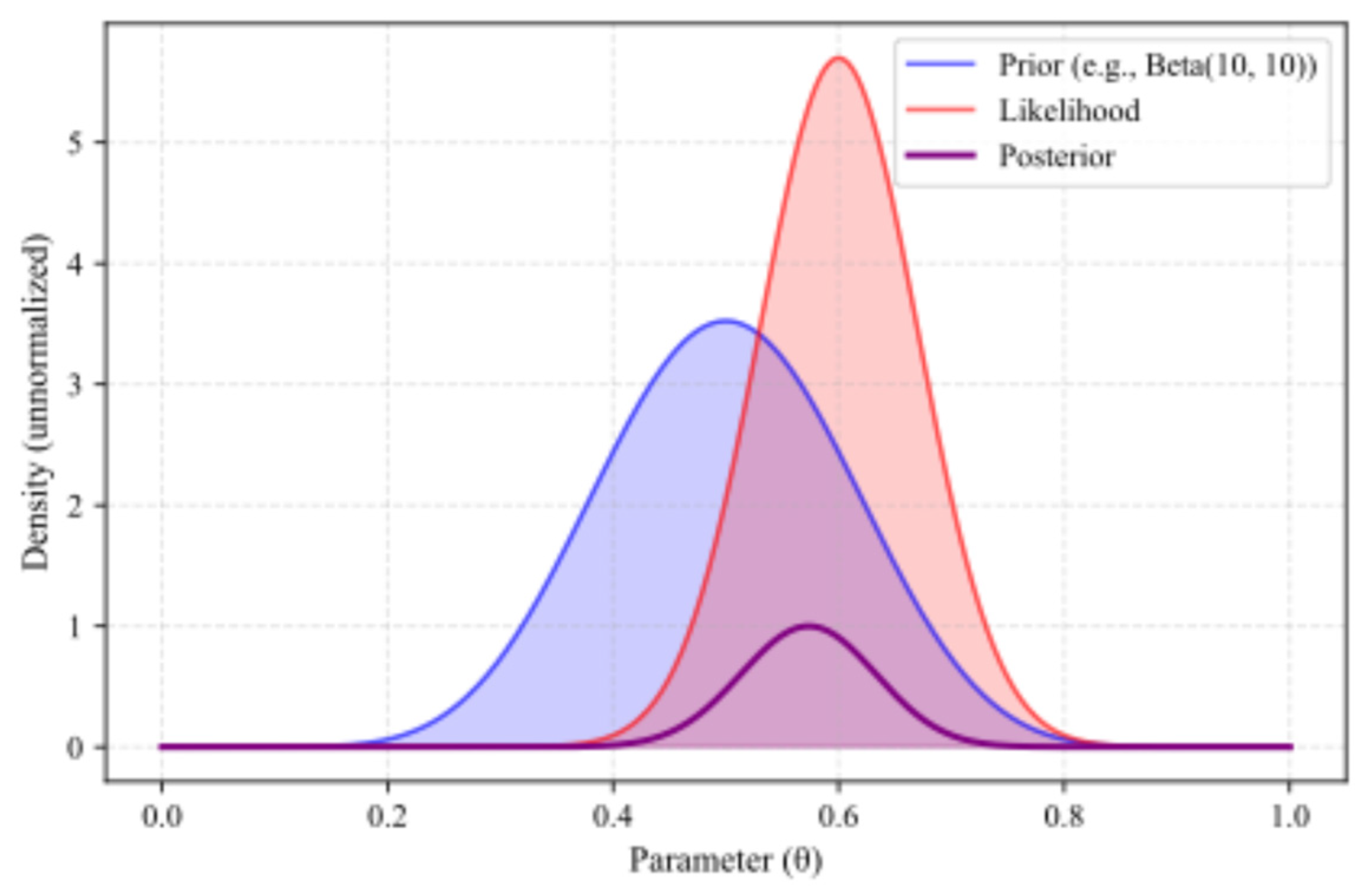
Figure 2.
Structure of a feedforward ANN with fully connected layers.
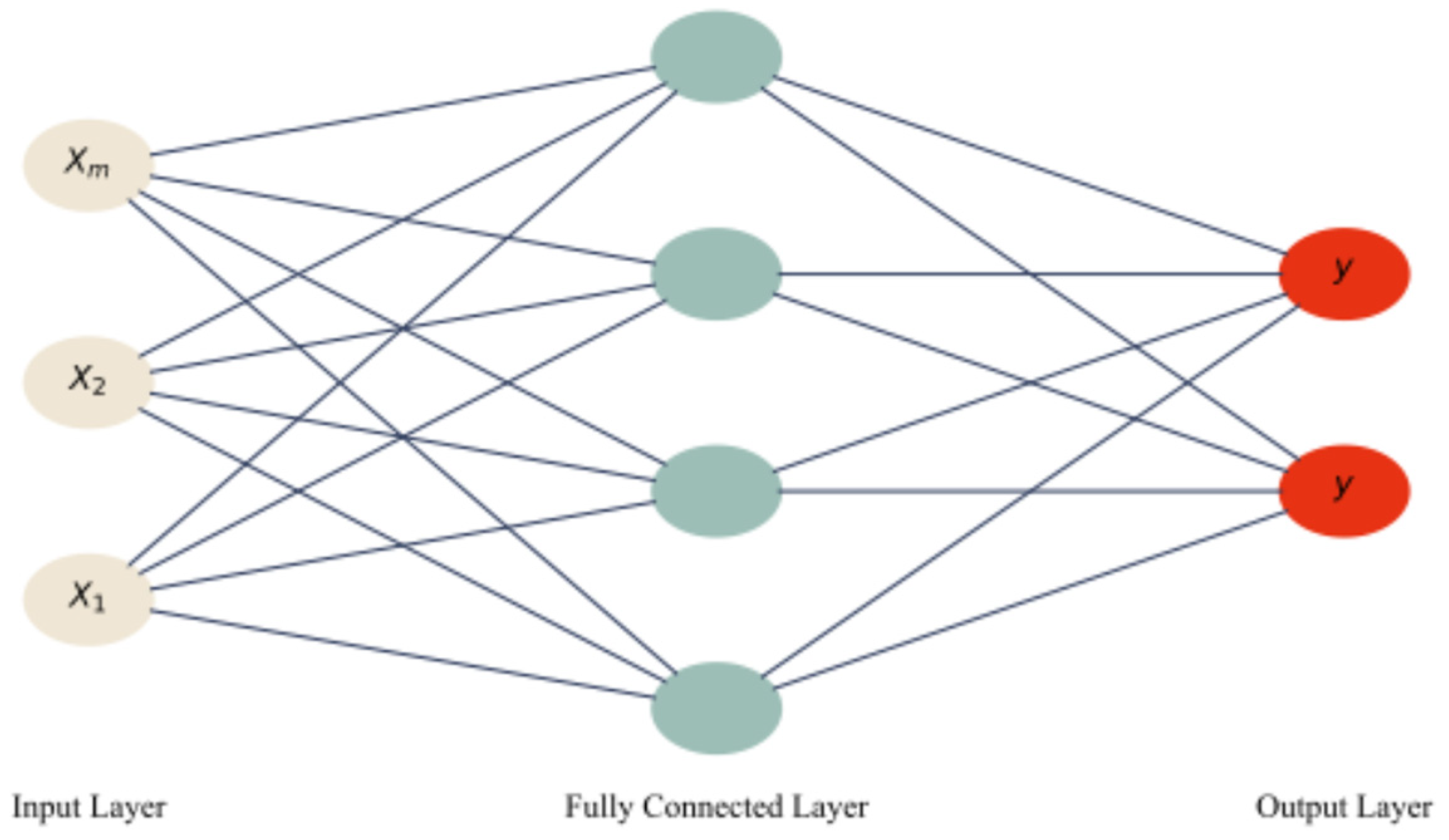
Figure 3.
SVM classification with decision boundary and margin visualization.
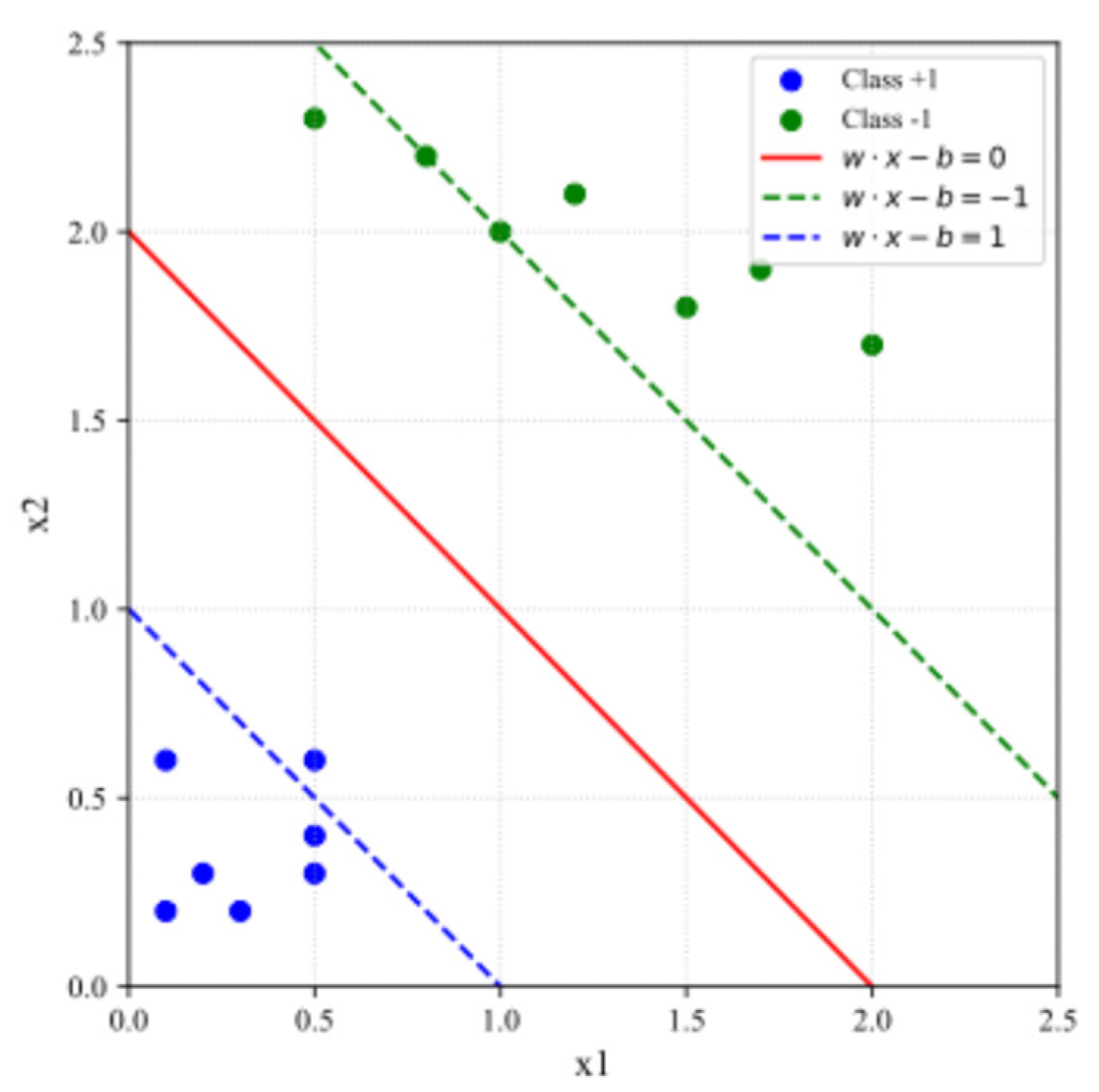
Figure 4.
Linear regression visualization.
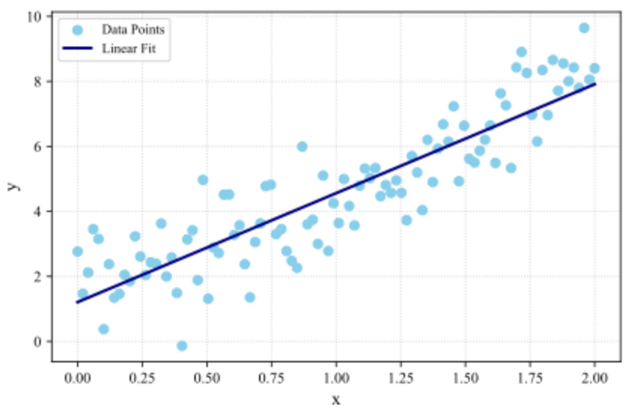
Figure 5.
Logistic regression classification curve and data distribution.
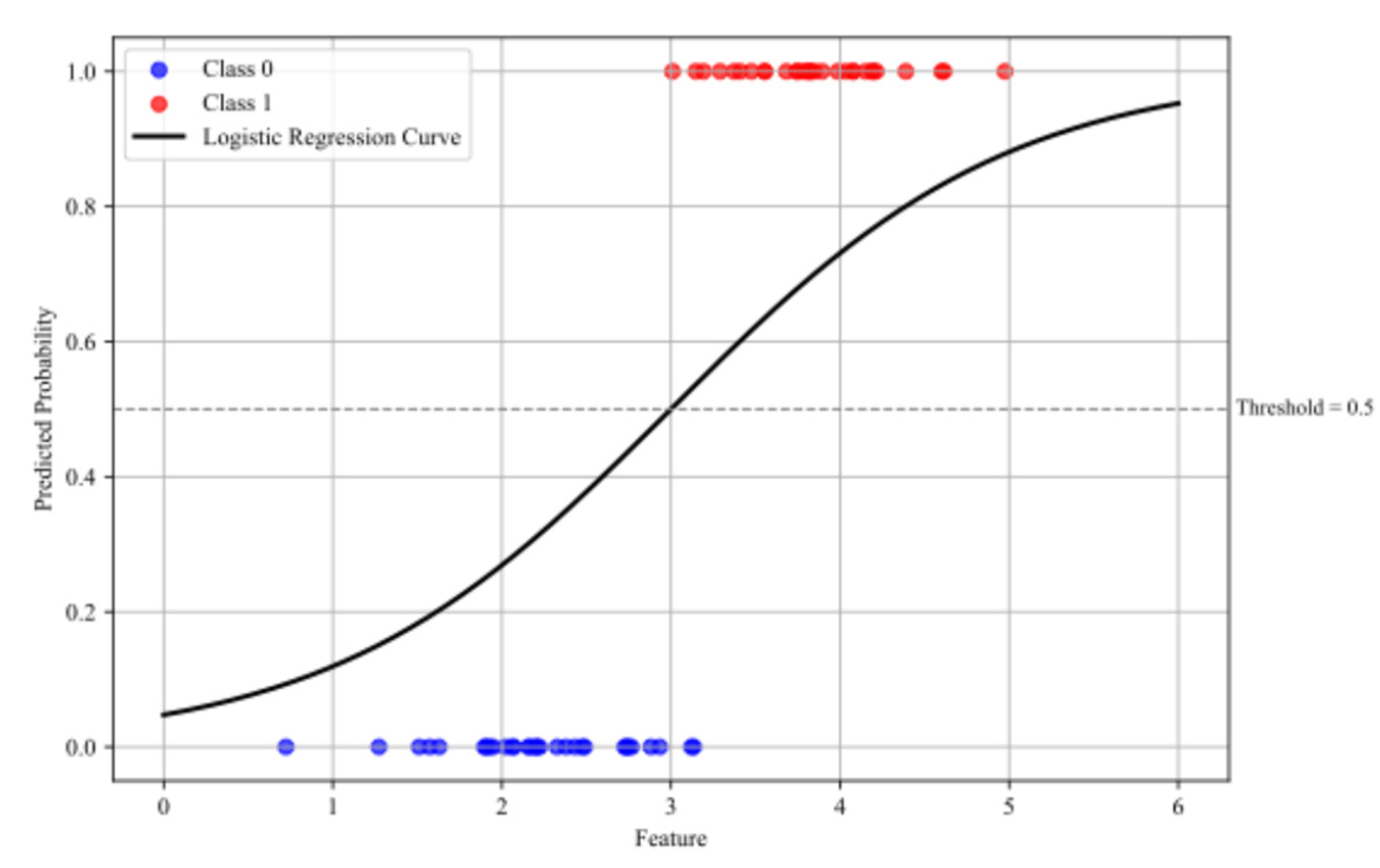
Figure 6.
Decision tree classification boundaries in a two-dimensional feature space.
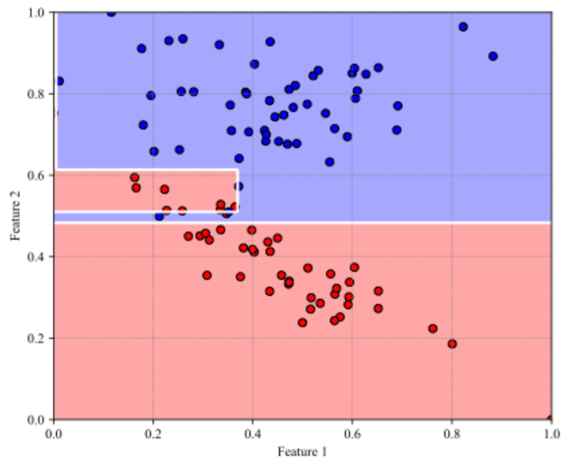
Figure 7.
Categorization of studies by dissemination type.

Figure 8.
Annual Distribution of Publications by Design Methodology.
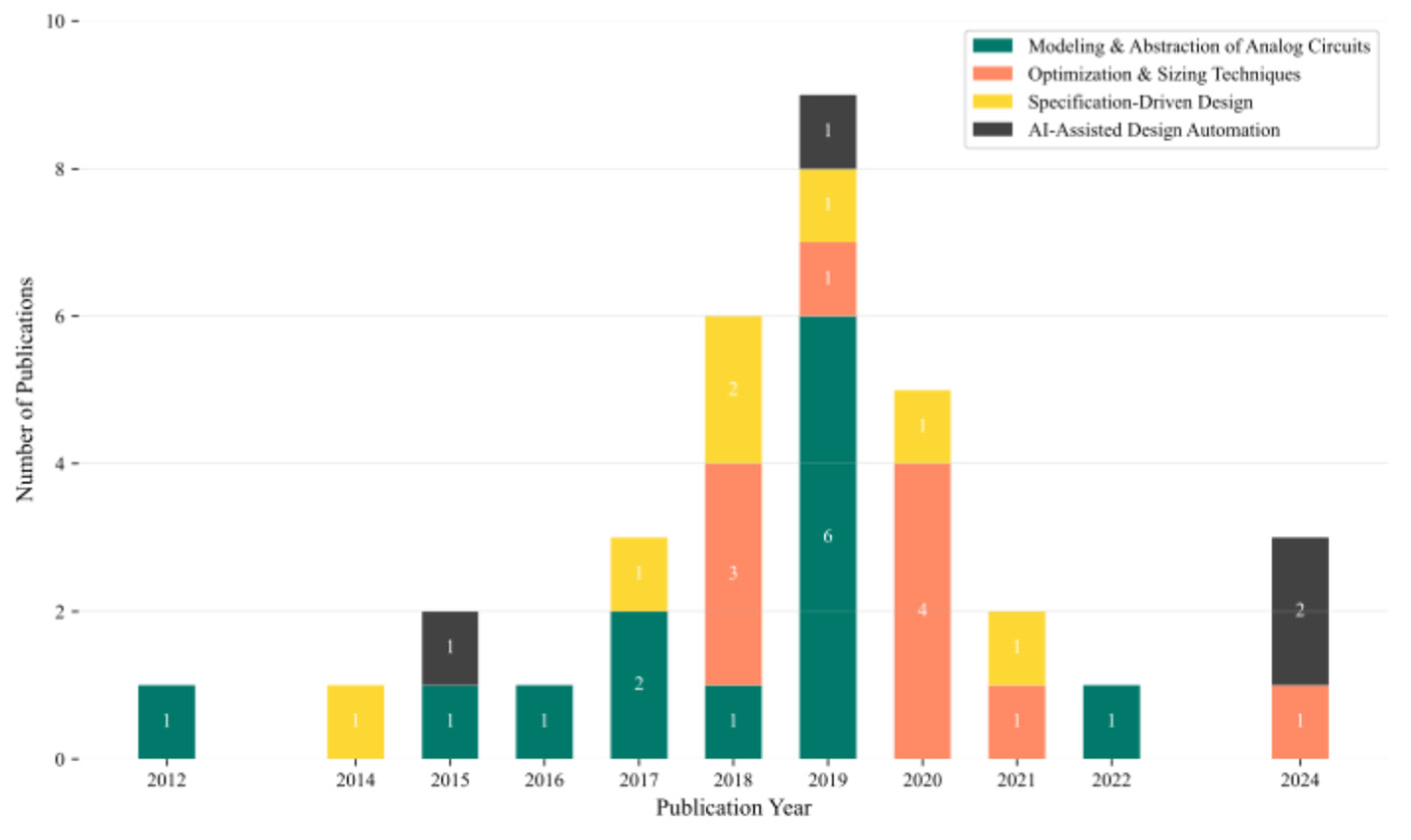
Figure 9.
Distribution of Journal and Conference Publications Across AMS-IC Design Methodology Categories.
Figure 9.
Distribution of Journal and Conference Publications Across AMS-IC Design Methodology Categories.
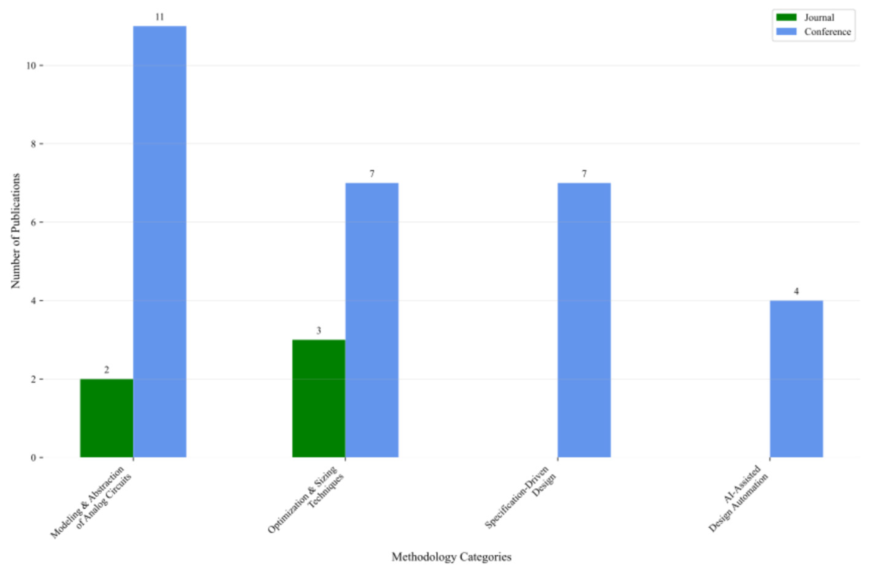
Figure 10.
(a) Distribution of AI/ML techniques in Modeling & Abstraction of Analog Circuits category; (b) Types of learning approaches used in Modeling & Abstraction of Analog Circuits category; (c) Prediction task in Modeling & Abstraction of Analog Circuits category.
Figure 10.
(a) Distribution of AI/ML techniques in Modeling & Abstraction of Analog Circuits category; (b) Types of learning approaches used in Modeling & Abstraction of Analog Circuits category; (c) Prediction task in Modeling & Abstraction of Analog Circuits category.
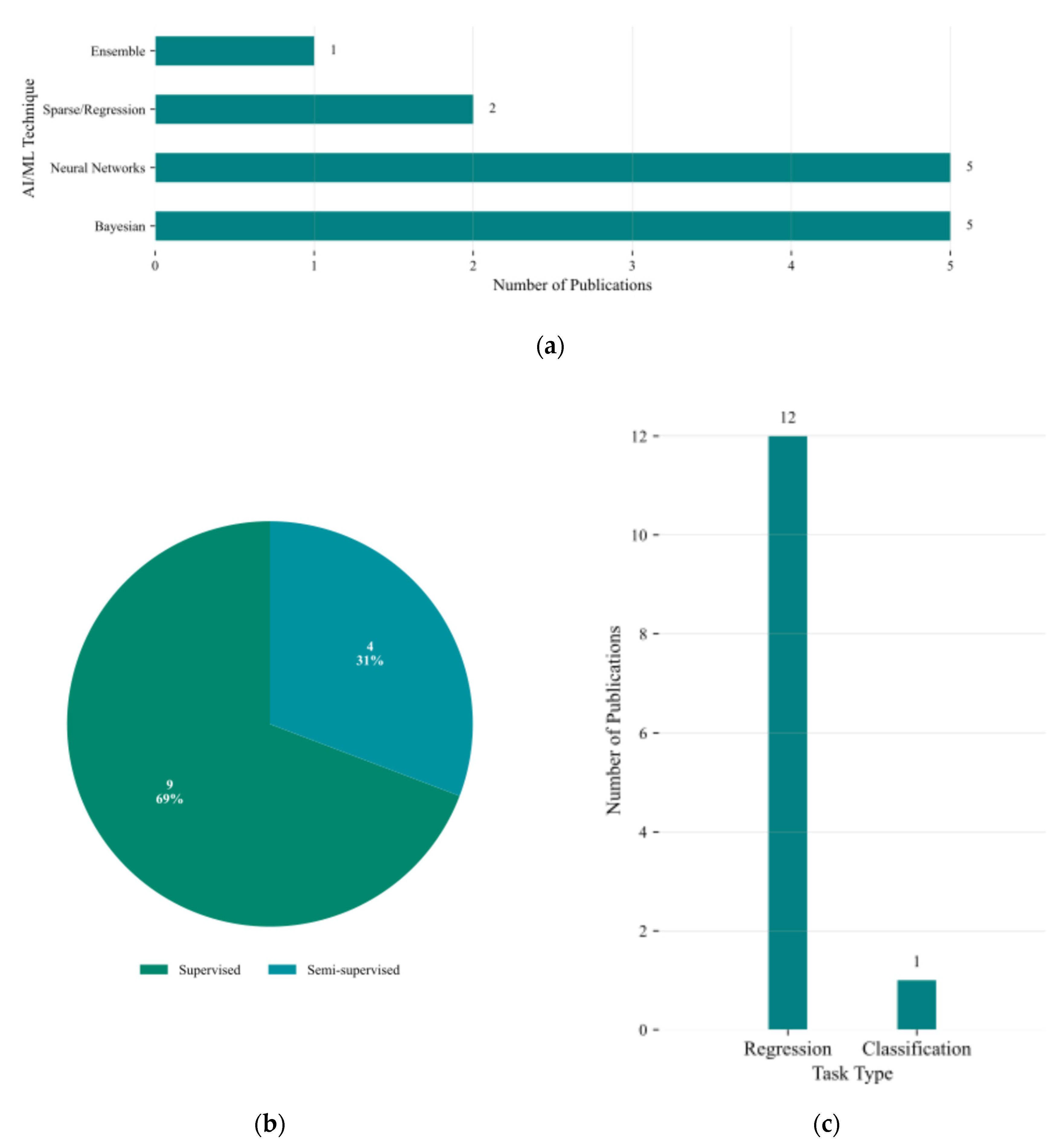
Figure 11.
(a) Distribution of AI/ML techniques in Optimization & Sizing Techniques category; (b) Types of learning approaches used in Optimization & Sizing Techniques category; (c) Prediction task in Optimization & Sizing Techniques category.
Figure 11.
(a) Distribution of AI/ML techniques in Optimization & Sizing Techniques category; (b) Types of learning approaches used in Optimization & Sizing Techniques category; (c) Prediction task in Optimization & Sizing Techniques category.
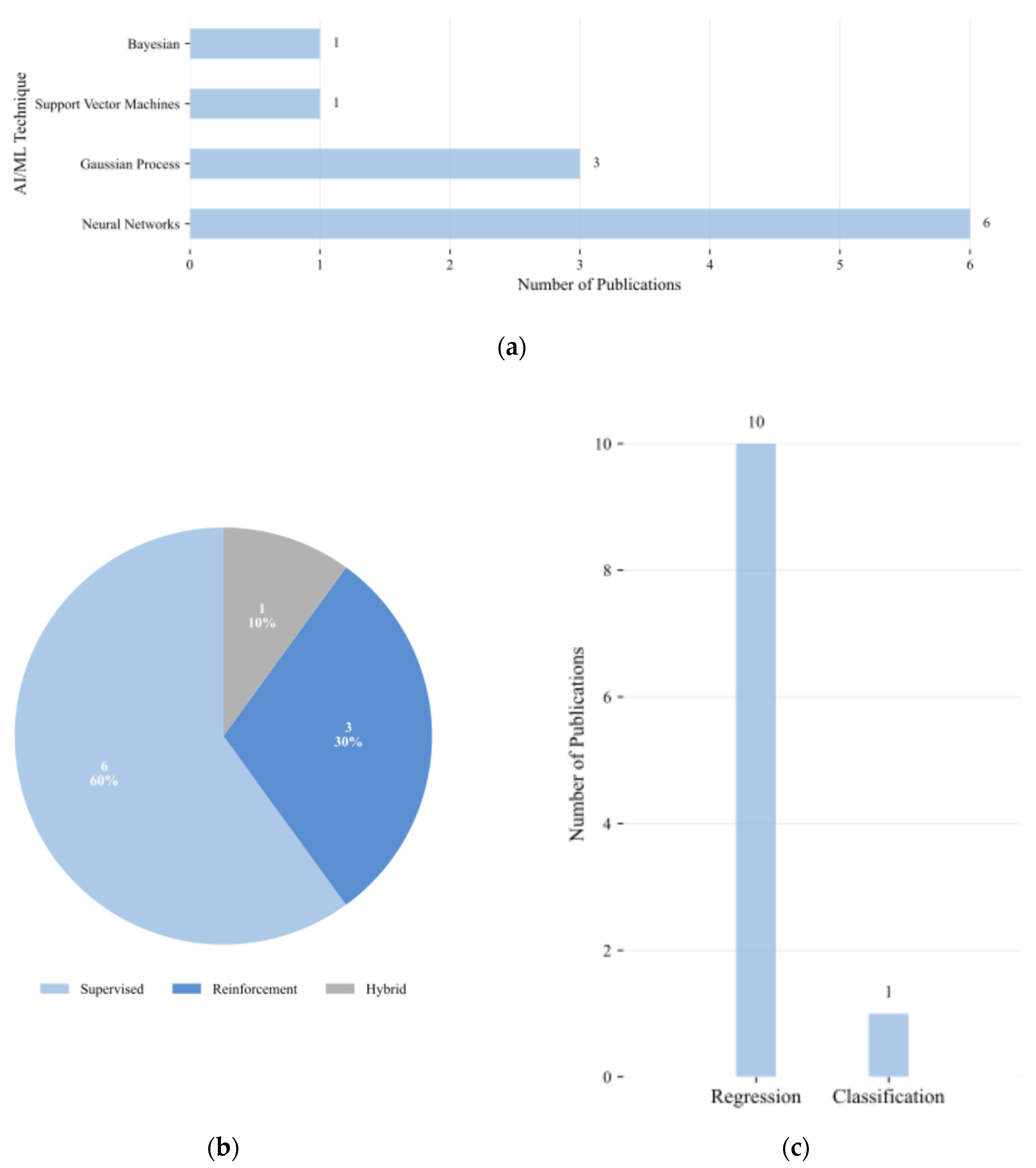
Figure 12.
(a) Distribution of AI/ML techniques in Specification-Driven Design category; (b) Types of learning approaches used in Specification-Driven Design category; (c) Prediction task in Specification-Driven Design category.
Figure 12.
(a) Distribution of AI/ML techniques in Specification-Driven Design category; (b) Types of learning approaches used in Specification-Driven Design category; (c) Prediction task in Specification-Driven Design category.
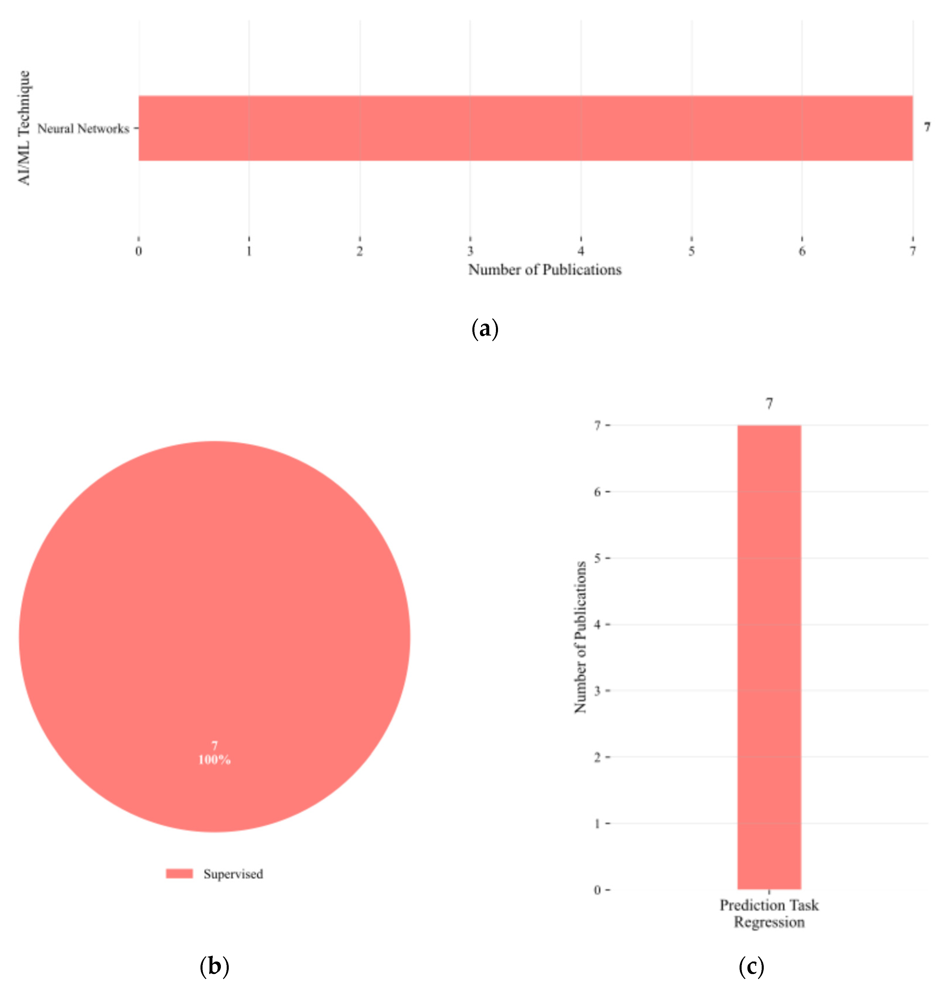
Figure 13.
(a) Distribution of AI/ML techniques in AI-Assisted Design Automation category; (b) Types of learning approaches used in AI-Assisted Design Automation category; (c) Prediction task in AI-Assisted Design Automation category.
Figure 13.
(a) Distribution of AI/ML techniques in AI-Assisted Design Automation category; (b) Types of learning approaches used in AI-Assisted Design Automation category; (c) Prediction task in AI-Assisted Design Automation category.
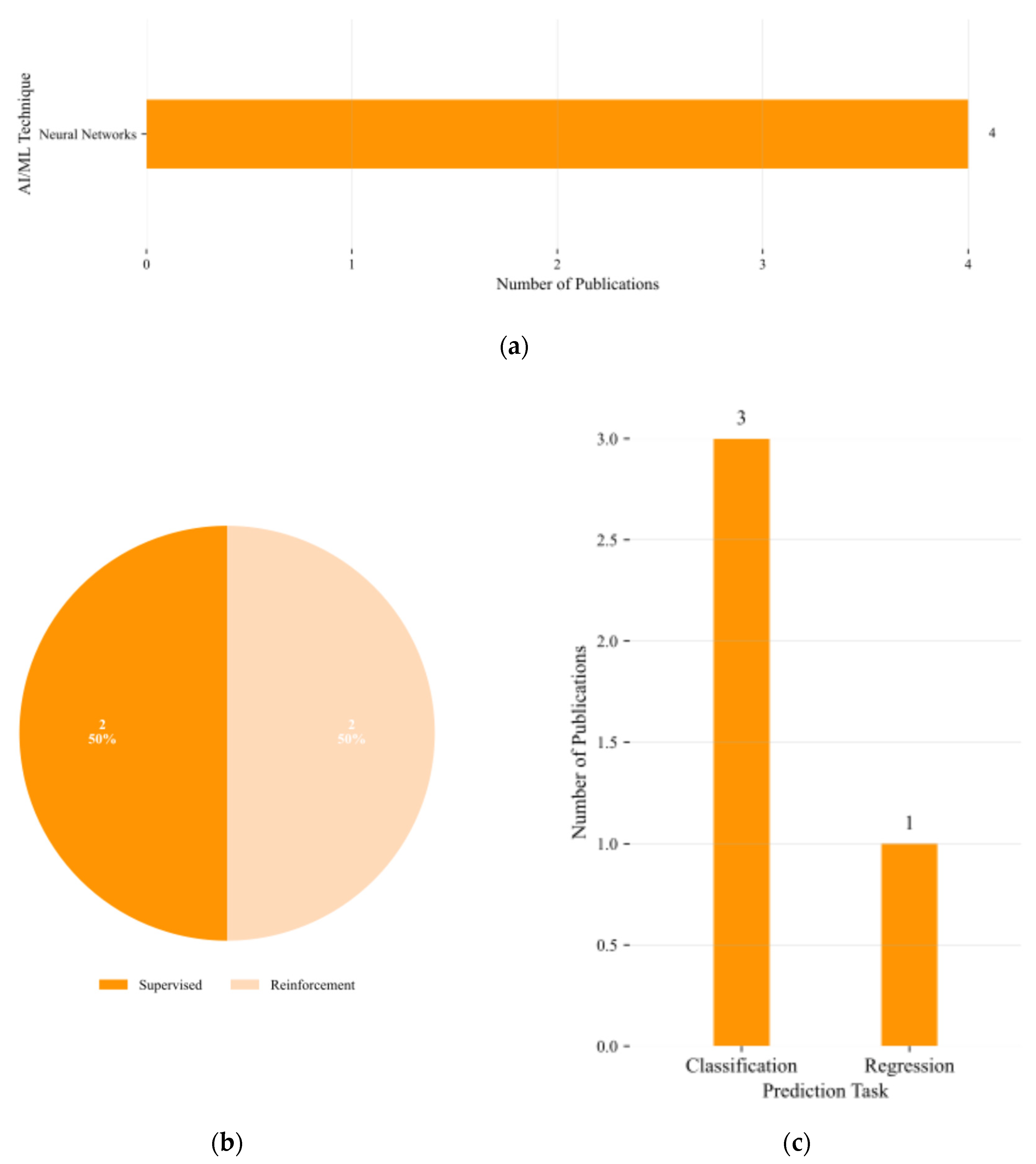
Figure 14.
Pie chart presenting the approaches according to each category.

Figure 15.
Distribution of AI/ML techniques.
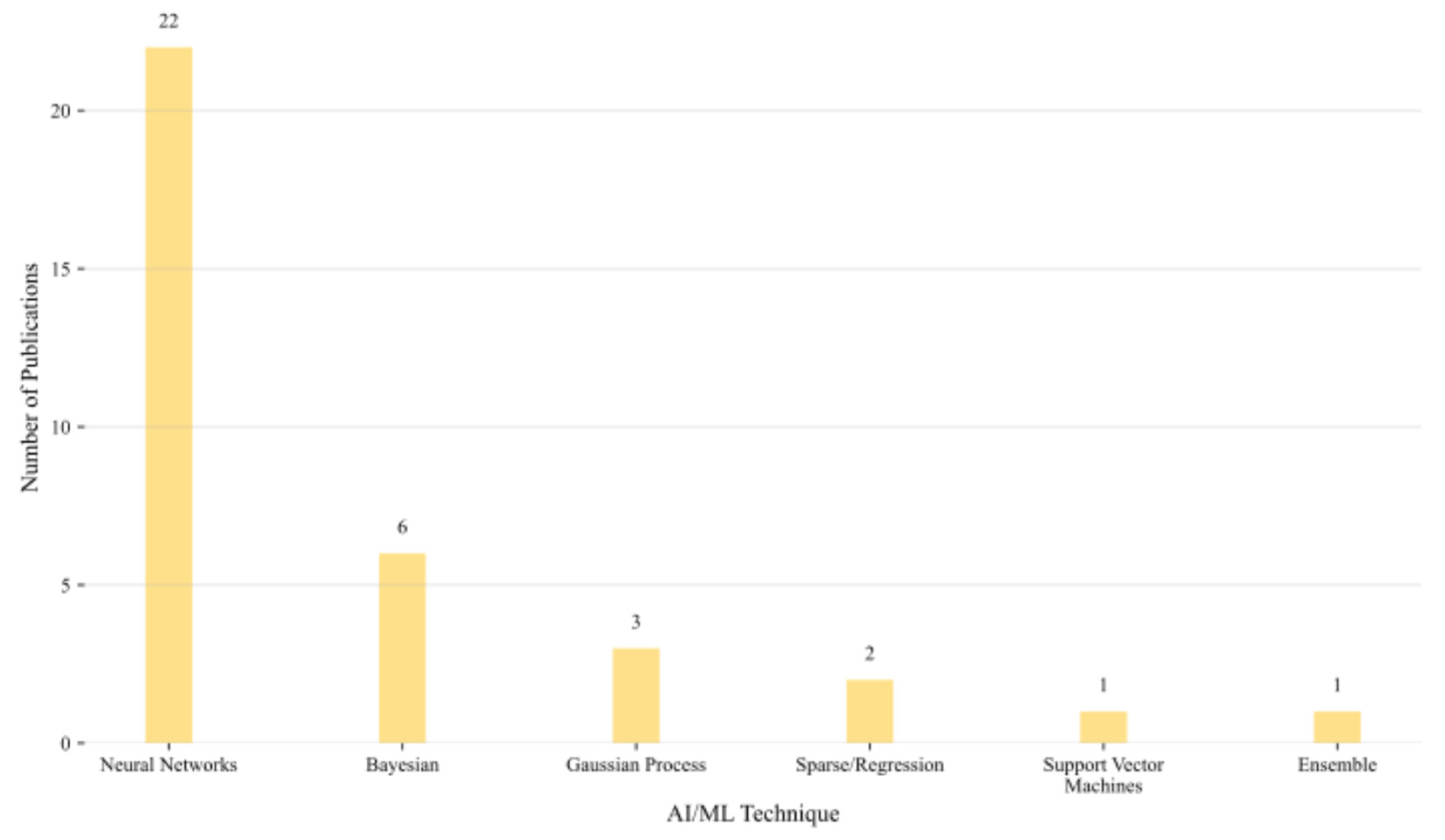
Figure 16.
Distribution of ML techniques across methodological categories.
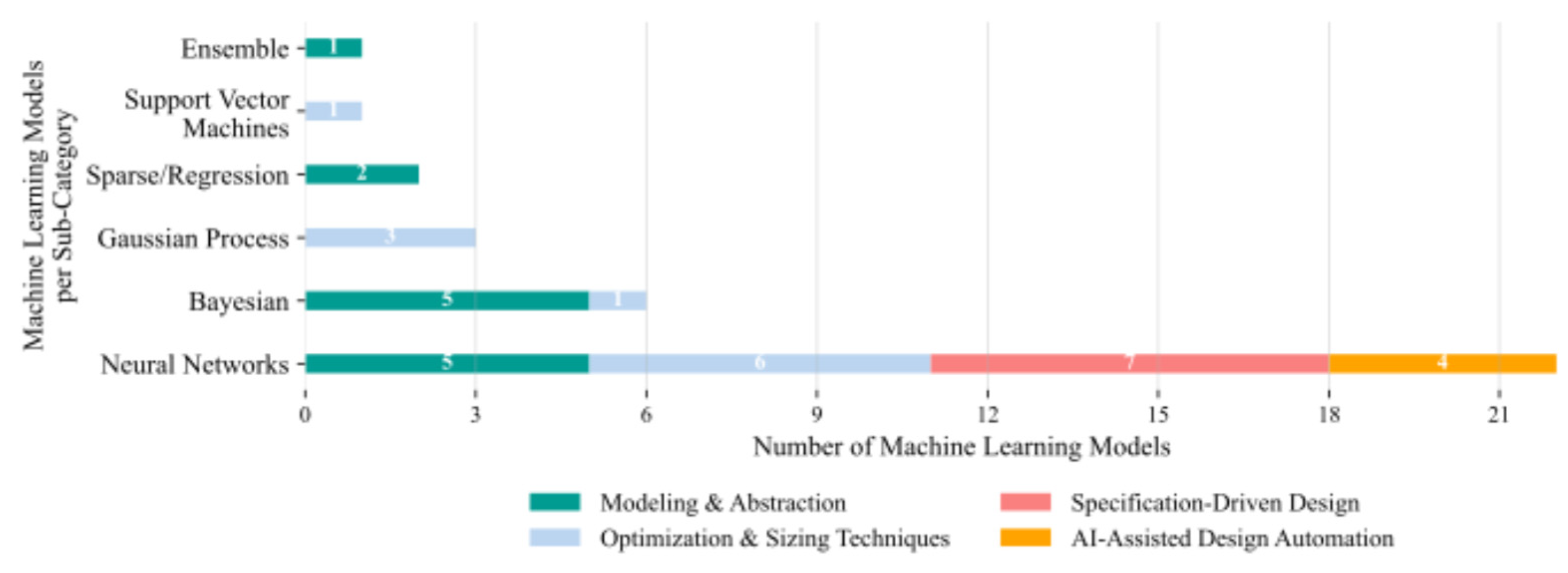
Figure 17.
Distribution of learning types across methodological categories.
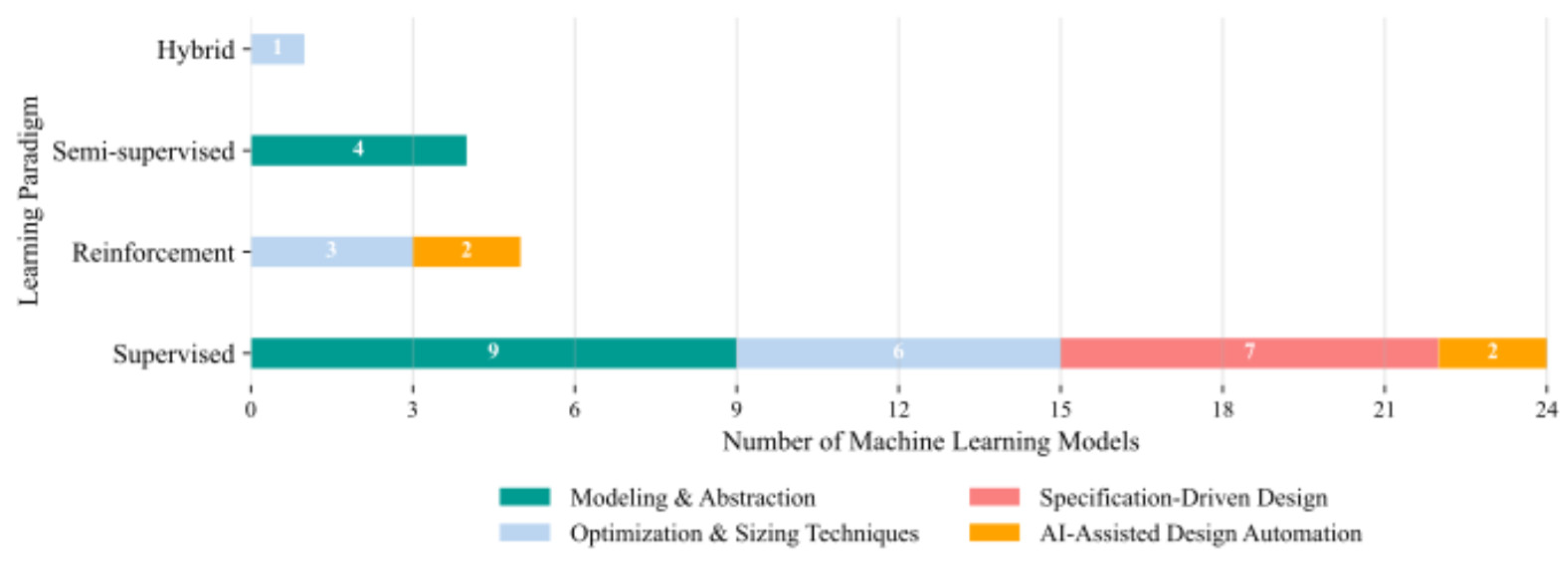
Figure 18.
Contribution of methodological categories per ML task type.
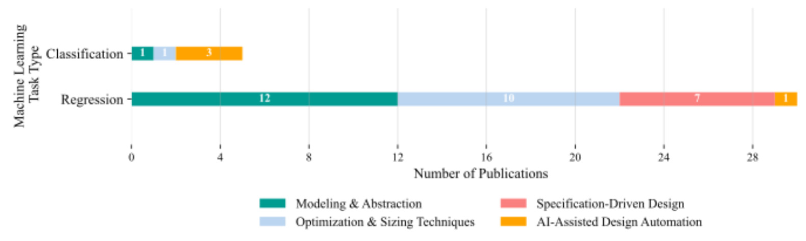

Table 1.
Summary of studies in Modeling & Abstraction of Analog Circuits category.
| Cite | Data Size | Observed Features | AI Method | Evaluation | Results |
| [38] | RO: 4000 samples SRAM: 1000 samples |
Power consumption, oscillation frequency, phase noise, and propagation delay | Semi-supervised BMF regressor | Prediction error | ~0.2 – 2% |
| [39] | RO: 750 fundamental frequencies and 10 phase noise samples, LNA: 13 forward gain and 1 noise figure samples |
Device-level process variations like, threshold voltage, oscillation frequency, noise figure, and forward gain | Semi-supervised CL-BMF regressor | Relative error | ~0.28 – 0.33 dB |
| [40] | Schematic: 3000 samples, Post-layout RO: 300 samples, Post-layout SRAM: 300 samples |
Device-level variations and layout extracted parasitics | Supervised BMF regressor | Relative error | < 2% |
| [41] | Trimming: 695 samples, Load jumps: 433 samples, Line jumps: 501 samples |
Trimming behavior and dynamic load/line transitions time-series signals | Supervised NARX and TDNN regressor | MSE, and Correlation coefficient (R) |
Trimming: 7e-5, Load: 5.6e-3, Line: 1.4e-3, R > 0.96 |
| [42] | Delay-line: 100 labeled and 300 unlabeled samples, Amplifier: 250 labeled and 450 unlabeled samples |
Propagation delay and power consumption across hierarchical circuit blocks | Semi-supervised BCL regressor | Relative error | Delay-line: 0.13%, Amplifier: 0.55% |
| [43] | Simulated-oriented programmable amplifier: 3,000–100,000 samples | Transistor sizing width & length, biasing parameters, voltage gain, and phase margin |
Supervised G-OMP regressor | No explicit modeling error metric reported | Authors confirm equivalent or improved solution quality |
| [44] | Charge pump: 200 samples, Amplifier: 260 samples |
Transistor width parameters and circuit-level performance metrics | Supervised BNN regressor | Hypervolume (HV) and Weighted gain (WG) |
Charge pump: 15.04 HV and 0.19 WG, Amplifier: 10.72 HV and 102 WG |
| [45] | Over iterative design generations: 20,000 samples | Transistor sizing ratios width & length, bias currents, and power consumption | Supervised FNN regressor | No explicit modeling error metric reported | Authors confirm ANN outputs closely match SPICE simulation results |
| [46] | Optical receiver: 435 samples, DNN queries: 77,487 samples |
Voltage gain, phase margin, diagram margin, and post-layout design specifications | Supervised DNN classifier | Sample compression efficiency | 300× |
| [47] | Operational amplifier: 130 samples, Charge pump: 890 samples |
Design specifications like, voltage gain, phase margin, transistor dimensions width & length, and passive components resistance, capacitance | Supervised Ensemble (BO|GP|NN) regressor | Figure of Merit (FOM) | Operational amplifier: FOM not reported Charge pump: 3.17 FOM |
| [48] | Labeled: 90 samples, Gibbs: 2800 samples |
High-dimensional process parameters targeting power performance | Supervised ANN regressor | Relative error | 2.39% |
| [49] | Comparator: 50 orthogonal matching pursuit (OMP) samples and 70 S2-PM samples, Voltage-controlled oscillator: 50 OMP samples and 40 S2-PM samples, Unlabeled: 20 samples |
Process variation parameters, including threshold voltage shifts | Semi-supervised Sparse regressor | Relative error | Comparator: OMP: 2.50%, S2-PM: 2.53% and Voltage-controlled oscillator: OMP: 1.55%, S2-PM: 1.6% |
| [50] | PySPICE: 4000 samples | Input impedance, voltage gain, power consumption, transistor dimensions width & length, and passive components resistance, capacitance | Supervised FNN regressor | MSE | 10⁻⁴ with ideal model, 10⁻² with PySpice |
Table 2.
Summary of studies in Optimization & Sizing Techniques category.
| Cite | Data Size | Observed Features | AI Method | Evaluation | Results |
| [51] | 24 parameters and 50,000 Monte Carlo simulations used for yield estimation | Design parameters, includes sizing, yield, and process corner metrics | Supervised BO–GPR regressor | Failure rate | 1% |
| [52] | Simulation budget of 100–1000 per circuit, including 20–40 initial design-of-experiment (DoE) samples | Design variables like, transistor sizes, passive dimensions, biasing levels and performance metrics like, gain, efficiency, area | Supervised BO–GPR regressor | No explicit modeling error metric reported | Demonstrated equal or superior Pareto quality with significantly reduced simulation cost |
| [53] | Operational amplifier: 500 samples, Power amplifier: 500 samples |
Includes performance specifications such as gain, phase margin, unity-gain frequency, power-added efficiency, and output power, along with design variables such as transistor dimensions, resistor, and capacitor values | Supervised BO–GPR regressor | No explicit modeling error metric reported | Demonstrated equal or superior Pareto front quality with 4–5× fewer simulations compared to non-dominated sorting genetic algorithm – II (NSGA-II) and genetic algorithm-based sizing of parameters for analog design (GASPAD) |
| [54] | Genetic algorithm: 260 population samples and 16 sampling segments | Device sizing parameters such as transistor geometry and biasing levels, along with performance metrics including gain, power, and bandwidth | Supervised BLR regressor and SVM classifier | No explicit modeling error metric reported | Demonstrated comparable or improved performance metrics with up to 1245%–1518% speed-up in circuit synthesis |
| [55] | Operational amplifier: 158 samples, Cascode band-pass filter circuit: 632 samples |
Includes transistor widths, resistances, and capacitances, along with performance metrics such as gain, unity-gain bandwidth, bandwidth, and phase margin | Supervised ANN regressor | Model error and R |
< 1% and 0.99 |
| [56] | 50,000 training tuples | Design variables such as transistor lengths, widths, and bias voltages, as well as performance attributes like DC gain, bandwidth, phase margin, and gain margin | Reinforcement PGNN regressor |
No explicit prediction error metrics reported | Model performance evaluated via convergence of the reward function, defined as a weighted combination of normalized DC gain, bandwidth, phase margin, and gain margin |
| [57] | Three-stage transimpedance amplifier: 40.000 SPICE samples, Two-stage transimpedance amplifier: 50.000 SPICE samples |
Circuit operating characteristics including DC operating points and AC magnitude/phase responses, along with transistor–level parameters such as threshold voltage, transconductance, and saturation voltage | Reinforcement DDPG regressor |
No explicit surrogate-model error metrics reported | Three-stage transimpedance amplifier: satisfied FOM score with a 250× reduction. Two-stage transimpedance amplifier: reached 97.1% of expert-designed bandwidth with a 25× improvement in sample efficiency |
| [5] | Transimpedance amplifier: 500 samples, Operational amplifier: 1000 samples, Passive-element filter: 40 samples |
Design objectives include gain, bandwidth, phase margin, power, and area, evaluated against design-space parameters such as transistor widths/lengths, capacitor values, and resistor values | Reinforcement DNN-PPO regressor |
No explicit surrogate-model error metric | Achieved 40 × higher sample efficiency than a genetic-algorithm baseline |
| [58] | Width-over-length sweep: 65.534 samples, Transconductance-to-drain-current sweep: 7.361 samples, GA-guided local refinement: 632 samples |
Design objectives include voltage gain, phase margin, unity-gain frequency, power consumption, and slew rate | Supervised ANN and Reinforcement DDPG regressors | Prediction score | Width-over-length sweep: 90%, Transconductance-to-drain-current sweep: 93%, GA-guided local refinement: 75.8% and DDPG 25–250× less sample-efficient than the supervised/GA pipeline |
| [59] | Five seed points plus twenty iterations, each evaluating one LLM-generated and four GP-BO candidates: 105 samples | Amplifier: 14 continuous design variables - all transistor widths / lengths plus compensation resistor Rz and capacitor Cc), Comparator: 12 continuous design variables - width and length of six transistors |
Supervised LLM-guided GP–BO regressor | No explicit surrogate-model error metric | Satisfies every design specification for both amplifier and comparator, achieves the top figure-of-merit among all methods, and reaches convergence with a 4 × reduction in optimization iterations |
Table 3.
Summary of studies in Specification-Driven Design category.
| Cite | Data Size | Observed Features | AI Method | Evaluation | Results |
| [60] | Low-noise amplifier: 235 samples | Bandwidth, 1-dB compression point, center frequency, third-order intercept point, noise figure, forward gain, transistor width/length ratio, source inductance, bias voltage | Supervised ANN regressor | Prediction accuracy | Matching networks: 99.22% accuracy, Transistor geometries: 95.23% accuracy |
| [61] | 20,000 samples after cleaning and normalization | Current and power consumption, direct current gain, phase margin, gain bandwidth product, slew rate, total harmonic distortion, common and power rejection ratio, output and input voltage range, output resistance, input referred noise |
Supervised FNN regressor | Average prediction accuracy | 92.3% |
| [62] | Original: 16,600 samples, Augmented: 700,000 samples |
Direct current gain, supply current consumption, gain–bandwidth, phase margin | Supervised ANN regressor | MSE and MAE |
0,0123 and 0,0750 |
| [63] | Not precisely specified, 5.000 – 40.000 samples |
Gain, bandwidth, power consumption | Supervised DNN regressor | Average match rate and RMSE |
95.6% and ≈30 |
| [64] | Pareto-optimal circuit sizing solutions: 700 samples | Load capacitance, circuit performance measures such as gain, unity gain frequency, power consumption, phase margin, widths and lengths | Supervised MP and ANN regressors | MAE | MP: 0.00807 and ANN: 0.00839 |
| [65] | SPICE: 7.409 samples | Gain, phase margin, unity gain bandwidth, area, slew rate, power consumption, widths and lengths of selected transistors, bias current, and compensation capacitor | Supervised ANN regressor | MSE and R2 |
≈ 4.26e-10 and 94.29% |
| [66] | LT-SPICE: 40.000 samples | DC gain, phase margin, unity-gain bandwidth, slew rate, area, compensation capacitor value and transistor widths, lengths, compensation capacitor, and bias current | Supervised FNN regressor | MAE | 0.160 |
Table 4.
Summary of studies in AI-Assisted Design Automation category.
| Cite | Data Size | Observed Features | AI Method | Evaluation | Results | ||||||
| [67] | Electroencephalogram segments: 4.098 samples | Frequency-domain energy in multiple bands and time-domain characteristics | Supervised ANN classifier | Accuracy, Recall |
≈96% and ≈95% |
||||||
| [68] | Post-layout simulated designs: 338 samples | Design parameters of an optical link receiver front-end in 14 nm technology, including resistor dimensions, capacitor dimensions, and transistor properties such as number of fins and number of fingers; performance metrics such as gain, bandwidth, and other specification errors | Supervised DNN classifier | No explicit surrogate-model evaluation metric reported | Specification-compliant design in 338 simulations, 7.1 hours, over 200× faster than baseline | ||||||
| [69] | Synthetic floorplans with 5–20 devices for training, 11-device circuit for evaluation, no explicit total sample count reported | Topological relationships between devices represented as sequence pairs; device parameters such as dimensions, shape configurations, symmetry, and alignment; performance objectives including occupied area and half-perimeter wirelength | Reinforcement DNN classifier |
No explicit model-level evaluation metric reported | Reduced refinement effort by 95.8%, and produced layouts 13.8% smaller and 14.9% shorter than manual designs | ||||||
| [70] | No explicit dataset size reported, multiple analog circuit topologies, including telescopic and folded cascode operational amplifiers | Gain, phase margin, power consumption, and slew rate, transistor dimensions, bias currents, and compensation capacitance | Reinforcement DNN regressor |
No explicit model-level evaluation metric reported | Fewer simulations, demonstrating higher sample efficiency in sizing multiple analog amplifier topologies | ||||||
Disclaimer/Publisher’s Note: The statements, opinions and data contained in all publications are solely those of the individual author(s) and contributor(s) and not of MDPI and/or the editor(s). MDPI and/or the editor(s) disclaim responsibility for any injury to people or property resulting from any ideas, methods, instructions or products referred to in the content. |
© 2025 by the authors. Licensee MDPI, Basel, Switzerland. This article is an open access article distributed under the terms and conditions of the Creative Commons Attribution (CC BY) license (http://creativecommons.org/licenses/by/4.0/).
Copyright: This open access article is published under a Creative Commons CC BY 4.0 license, which permit the free download, distribution, and reuse, provided that the author and preprint are cited in any reuse.


