
Submitted:
28 May 2025
Posted:
29 May 2025
You are already at the latest version
Abstract
The Gaussian Process Regression (GPR) has emerged as a state-of-the-art machine learning approach, offering significant potential for reducing testing costs in large-scale integrated circuits (LSIs) while maintaining high-quality standards. This study focuses on the wafer-level characteristic estimation, which measures a small subset of LSI circuits and estimates the characteristics of unmeasured ones. Additionally, it investigates the delay information estimation of field-programmable gate arrays (FPGAs) using ring oscillators (ROs) in look-up tables (LUTs). A key novelty of this work lies in addressing the critical challenge of kernel function selection, an essential factor in applying GPR to LSI testing and FPGA delay prediction. Through experimental analysis on mass-produced LSI industrial production data and actual measured silicon data, this research evaluates proposed adaptive custom kernel functions to identify optimal configurations. The findings reveal that, although hybrid and composite kernel architectures integrating multiple high-accuracy kernels outperform individual kernels in terms of accuracy, they are not consistent across different platforms. The proposed adaptive kernel consistently delivers improved prediction accuracy across multiple platforms, as demonstrated using industrial production data and actual measured silicon data.
Keywords:
Multi-site RF IC Testing
; Gaussian Process Regression
; Wafer-level Variation Modeling
; Kernel Function
; Die Selection
; FPGA
; Adaptive Kernel
1. Introduction
Large-scale integrated circuits and field-programmable gate arrays are receiving significant attention in modern technology. Many sectors, from automotive to healthcare, rely heavily on these technologies. While LSIs offer high-density integration and optimized performance, FPGAs provide flexibility and reconfigurability, making them complementary technologies in many applications [19,21,22,23,24,31]. Given their critical role, ensuring device reliability through comprehensive testing has become paramount, as faulty devices can significantly impact system operations and societal functionality. This necessitates extensive testing across various manufacturing stages under diverse conditions [30]. As these semiconductor devices increase in complexity and functionality, the volume of required tests has surged, resulting in higher test costs. This increasing expense is a major concern, as testing now constitutes a substantial portion of the overall manufacturing cost for both LSIs and FPGAs [2,3,4,5,12]. The challenge of maintaining thorough testing while managing costs is particularly pronounced in FPGAs, where the reconfigurable nature of the device adds an additional layer of complexity to the testing process. Various test cost reduction methods have been proposed that apply data analytics, machine learning algorithms, and statistical methods [16,22,25,26,28,32,22]. In particular, wafer-level characteristic modeling methods based on statistical algorithms are the most promising candidates that reduce test cost, that is, measurement cost, without impairing test quality. [1,15,16,17,20,35,37].
On the other hand, the state–of–the–art FPGA estimation proposed in [4] shows that the estimated measurements can be drastically reduced through a compressed sensing-based virtual probe technique [36]. However, as experimentally shown in [25], in experiments conducted using wafer measurement data from a mass industry production, the Gaussian process (GP)-based estimation method surpasses the techniques presented in [4], which are based on compressed sensing [7]. Because estimation eliminates the need for measurement, it not only reduces the cost of measurement, but can also be used to reduce the number of test items and/or change the test limits, which is expected to improve the efficiency of adaptive testing [13,18,27,34]. In [20], the expectation maximization (EM) algorithm [10] was used to predict the measurement. The Gaussian process-based method provides more accurate prediction results [25]. The use of GP modeling has another side benefit. As it calculates the confidence of a prediction, the user can confirm whether the number and location of measurement samples are sufficient, and suitable or not, being a great advantage from a practical viewpoint. In addition, since the GP can calculate the uncertainty of the estimation result, the user can confirm whether the number and location of measurement samples are sufficient and suitable or not.
Figure 1 presents an experimental analysis in the form of a heat map, showing the full measurement results for a wafer of a 28 nm analog /RF device, with estimation based on 10% of the training data. The figure includes three heat maps (a, b, c), where (a) represents the actual measured data, while (b) and (c) show the predicted data using a virtual probe and Gaussian process regression (GPR), respectively. In both cases, 10% of the samples are used to estimate the remaining 90% of the unmeasured samples. It is evident from the figure that both VP and GPR effectively address and accurately predict the unknown measured data with high accuracy and minimal error.
Figure 2 shows a similar experiment with delay information in look-up tables (LUTs) using ring oscillators (ROs). The figure includes three heat maps (a, b, c), where (a) represents the actual measured data, while (b) and (c) show the predicted data using a 10% virtual probe and 10% training data for the Gaussian process regression (GPR), respectively. The figure shows the similar trend on Figure 1 and in both cases VP and GPR effectively address as well as accurately predict the unknown measured data with high accuracy and minimal error.
The VP technique exploits the sparsity of frequency-domain components in spatial process variation for prediction. Due to the gradual nature of process variation in FPGAs and wafers, high-frequency components approach zero, allowing seamless integration with fingerprinting techniques. The method’s effectiveness is validated through silicon measurements on commercial FPGAs.
Unlike VP’s direct frequency-domain approach, GPR models spatial process variation as a probabilistic distribution using kernel-based correlation analysis. This technique effectively handles gradual variations through Gaussian process smoothing, making it ideal for probabilistic predictions. Experimental validation using commercial FPGAs and wafer analog/RF device data demonstrates the method’s effectiveness [1,8,9,29,33].
However, when applying GPR, it is most important to select the best kernel function, but the appropriate kernel function for LSI testing is not well understood. Since there is no effective method for investigating kernel function selection, this study applies GPR to mass production LSI test data, experimentally compares a large number of kernel functions, and identifies the best kernel function. Furthermore, based on this evaluation, this study also demonstrates that estimation accuracy can be further improved by using multiple kernel functions with high estimation accuracy. The hybrid or mixture kernels are proposed in [6,8,9,11,29] where different modes of mixing and combining are explained. In [11], sum of two product kernels achieves a best result among all individual kernels.
Most importantly, even when a single kernel or composite kernel function works well, it may not outperform others in different datasets with similar performance. Additionally, composite or adaptive kernels with too many parameters may suffer from overfitting issues. This study aims to determine a custom adaptation based on prediction confidence to select the top two candidates for adaptation with dynamic weight adjustment based on the estimation confidence, instead of using fixed-weight adaptive kernels. Unlike typical hybrid or mixture kernels proposed in [6,8,9,29], this approach determines the weight of each kernel based on their difference in confidence levels. After an exhaustive analysis of various kernel functions across all possible combinations, using actual industry production data and real silicon data, it was observed that the proposed custom-adaptive kernel consistently outperformed across two different datasets.
The remainder of this paper is organized as follows: Section 2 provides an overview of GP-based modeling for wafer and FPGA process variations. Section 3 details the kernel function and proposed custom-adaptive kernel strategies. Section 4 presents a quantitative evaluation of the proposed custom kernel approach compared to conventional approaches. Finally, Section 5 offers the conclusion.
2. Gaussian Process Regression for Semiconductor Reliability
To better understand the origin and structure of the data used in our Gaussian Process Regression (GPR) modeling, we first provide an overview of the physical and logical architecture of FPGAs and wafer-level layouts.
2.1. Basic Structure
Figure 3 presents an annotated layout that bridges both the logical structure of an FPGA and the physical organization at the wafer level. Within each chip, Configurable Logic Blocks (CLBs) serve as the core computational units and are arranged in a regular grid pattern. Each CLB is composed of Look-Up Tables (LUTs), flip-flops, and carry chains, allowing the implementation of diverse digital logic through reconfigurable interconnects. These elements are connected via a combination of switch blocks and connection blocks, which form the programmable routing fabric. I/O blocks positioned around the perimeter enable external communication.
From the wafer-level perspective, each chip is bounded by scribe lines—regions without circuitry used as cutting paths during the dicing process to separate individual chips. Adjacent to the main dies, Test Element Groups (TEGs) are placed to validate process consistency and chip behavior during manufacturing. The wafer edge includes a flat zone, a small flattened segment used for alignment during lithography and testing. Together, these components contextualize how logic resources are mapped within a chip and arranged across a wafer for fabrication, validation, and testing purposes. A kernel function is a key component of Gaussian Process Regression (GPR) used to measure similarity between input data points. It defines the covariance structure of the data, enabling GPR to model complex patterns. Common examples include: the Linear kernel , Polynomial kernel , and Gaussian kernel
. The Radial Basis Function (RBF) kernel, a widely used variant, is given by . Each kernel introduces different assumptions about smoothness and locality, influencing the predictive behavior of the GPR model.
2.2. Gaussian Process Regression
A Gaussian distribution is a type of probability distribution for continuous variables, also known as a normal distribution. In this distribution, the mean, mode, and median are identical, and the distribution is symmetric around the mean. Since it is continuous rather than discrete, the distribution is represented as a smooth curve rather than a histogram. The probability density function of the Gaussian distribution is given by:
where represents the expected value (mean) and denotes the standard deviation.
The probability distribution treats the function as a random variable, creating a probabilistic model that predicts y for a given input x. When is defined, the outputs for inputs follow a Gaussian process. The joint distribution of at any set of points is Gaussian. This property holds true even as N approaches infinity, making a Gaussian process an infinite-dimensional Gaussian distribution.
As illustrated in Figure 4, Gaussian process methods are used to model the relationship between input X and output Y. This relationship is expressed mathematically as:
where represents the model’s noise or uncertainty. Data collected from the Wafer and FPGA are used to establish this relationship. Using this model, we can estimate the new output for both Wafer and FPGA is the new input data . The model is constructed as a function of the probability distribution using Bayesian inference.
As mentioned earlier, the semiconductor industry is pursuing methods to improve quality without increasing test costs, or to reduce costs while maintaining quality. Particularly for the latter, wafer-level characteristic modeling methods based on statistical algorithms yield good results. This model uses Gaussian process regression for prediction, creating a prediction model based on limited sample measurements on the wafer surface or FPGA lookup table to predict the entire wafer surface and entire lookup tables.
Figures [Figure 5] (a-c) illustrate how the model the relationship between input x and output y. Data D is utilized to model the relationship. The new output y(n+ 1) for the new data x (n+ 1) is estimated based on the model. The model is calculated as a function of the probability distribution with the Bayesian manner.
3. Proposed Custom-Adaptive Kernel Approach
The GP-based regression employs kernel functions from the GPy [14] framework to model and predict the characteristics of wafers and FPGAs.
This method learns from the measurement results of a small number of wafers’ characteristics and FPGA delay information. After the learning phase, it determines two functions: , which relates to the wafer LSI coordinates, and , which relates to FPGA delay information in look-up tables (LUTs) using ring oscillators (ROs). These functions estimate the characteristics of unmeasured wafers and FPGAs.
Let represent the wafer surface coordinates, and represent the FPGA LUT delay information. Similarly, define and as the respective measurement values to be predicted.
The training and test datasets are defined as follows:
For wafer data:
For FPGA data:
where and .
Using the predictive models and obtained from GPR, the predicted values for the test datasets are:
3.1. Hybrid or Mixture Kernel Strategy
The Hybrid or Mixture Kernel approach combines multiple kernel functions, each tailored to specific data characteristics, into a composite kernel. This strategy traditionally uses fixed weights for individual kernels, expressed as:
where are the individual kernels, and are their static weights with . However, such static weighting lacks adaptability to varying data properties, limiting robustness and flexibility. Although there are several ways to select the number of kernels and assign their weights, a common approach is to distribute the weights equally. For example, if two kernels are used, each is assigned a weight of 0.5; similarly, if four kernels are used, each receives a weight of 0.25.
3.1.1. Adaptive Kernel Strategy
Unlike the hybrid kernel strategy, the adaptive kernel strategy dynamically adjusts weights based on kernel performance metrics, thereby enhancing flexibility and robustness.
This strategy aims to improve GPR’s adaptability across wafer and FPGA data by adjusting kernel influence dynamically. Let the dataset be represented as:
where each is a measured input–output pair from a probe point. The candidate kernels are modeled as:
where denotes the regression model trained using kernel . Kernel performance is evaluated using validation errors:
These are used to determine kernel ranking and influence in the final model.
3.1.2.1 Composite Adaptive Strategy
This strategy considers performance differences and a threshold to determine whether reweighting is necessary. It is effective when kernel performance is close and noise robustness is desired.
Let denote the performance score of kernel k, and define the top three indices as:
Let represent pairwise performance differences. The composite kernel is defined as:
Where K1, K2, K3, K4 are the top four candidate kernels respectively.
Weights are assigned as:
The final composite kernel is:
3.1.2.2 Aggressive Adaptive Strategy
This simplified strategy omits thresholding and assigns weights directly based on kernel ranking. It is suitable when kernel performance gaps are consistently clear.
The composite kernel is defined as:
Weights are assigned as:
3.2. Proposed Custom-Adaptive Model
Before discussing the proposed custom adaptive strategy, we first analyze the correlation between predictive variance and average error, as illustrated in Figure 6 and Figure 7. These figures show the scatter plot of predictive variance versus average error, and the cumulative mean of average error versus predictive variance, for the Matern52 and the Linear kernel, respectively. In both figures, Gaussian Process Regression (GPR) is used to predict the input data using a randomly selected 10% of the samples for training, with error calculated as defined in Equation 17 in Section 4. The variance versus average error scatter plot and the cumulative mean of average error versus variance illustrate this relationship under different kernel behaviors.
Although lower predictive variance is often associated with reduced prediction error, certain regions exhibit deviations due to underestimation of uncertainty, particularly in sparse or non-representative test samples. In the case of the Matern-52 kernel, the error remains consistently low, with the cumulative trend exhibiting a slight increase as variance grows. The scatter plot demonstrates a weak positive trend where higher variance corresponds to slightly lower errors. For the linear kernel, where the prediction uncertainty is higher, the correlation exhibits a stronger negative trend. In both cases, regardless of the kernel choice, the negative correlation establishes that lower variance is associated with lower error. A similar trend is also examined in wafer data. We examined a negative correlation between the cumulative average error and the predictive variance. Although in some cases, such as for certain wafer and FPGA paths, we observed a positive correlation for some kernels, the overall correlation averaged across the datasets was found to be negative in both cases.
Considering this relationship, the proposed custom adaptive strategy is depicted in Figure 8. The figure illustrates how kernel weights are adapted based on confidence levels derived from the variance. In this approach, the kernel weights are calculated based on predicted variance instead of during the estimation process.
Figure 8 presents the different datasets
with different kernel functions . Here, each represents an individual wafer in the case of wafer data (i.e., wafers within a lot), and a specific path in the case of FPGA data (i.e., delay paths measured across devices). The Gaussian Process Regression (GPR) estimates the variance for each kernel function. Based on these variance estimates, the top two kernel candidates and are selected using the criterion of lowest average predictive variance across all datasets.
The weights and are defined to satisfy the following condition:
where the weights are assigned based on the difference in the variances and :
The weight is calculated as:
where is a scaling factor to control the impact of the variance difference on the weight.
Similarly, is given by:
Here, if , then and as the variance difference increases, increases if and decreases if . The smaller the variance of compared to , the more dominates.
This approach ensures that the kernel with higher confidence level receives greater weight, reflecting its importance in the combined kernel function. The proportional adjustment of and accommodates scenarios where one kernel significantly outperforms the other in terms of variance.
Figure 9 illustrates the relationship between the kernel weights , , and the variance difference . It consists of a general plot showing how the weights shift as changes, and an example inset demonstrating the calculation for two specific variances: 10 and 5. For example, the calculation for kernel weights (with scaling factor ) is as follows:
Consider two kernel predictive variances, 5 and 10. The variance difference is calculated as . Using the variance-based weighting strategy, the kernel with lower variance (5) is assigned a higher weight:
Thus, the resulting weights are and , as shown in Figure 9.
The proposed weighting mechanism adjusts and based on the variance difference between the two kernels. This hypothesis provides a robust framework for assigning weights, ensuring that kernels with lower variance contribute more to the combined kernel function.
4. Experimental Result
In this study, we conducted experiments using two different computational environments tailored to two distinct datasets. The wafer data was processed on a Linux workstation running Debian with an Intel Core i7 processor and 32 GB of memory. In contrast, the FPGA data was analyzed on a Windows 11 workstation equipped with an AMD processor and 16 GB of memory.
The kernel selection strategy, as summarized in Table 1, adopts a systematic methodology: (1) Hybrid kernels combine the top two performers (MLP and Exponential for wafer data; RatQuad and Matern52 for FPGA) based on preliminary error evaluations (see Tables 2–3); (2) Adaptive kernels incorporate four high-performing kernels—MLP, Exponential, RBF, and OU for wafer; Matern52, RatQuad, Matern32, and Exponential for FPGA; (3) Proposed Custom Adaptive kernels utilize the top two candidates (Exponential + RBF for wafer; Matern52 + Exponential for FPGA), selected dynamically via a variance-based weighting scheme, as outlined in Section 3.2 (Eqs. 13–16).
4.1. Experimental Setup
This section outlines the experimental setup used to evaluate the proposed custom-adaptive kernel method, along with a summary of existing studies on kernel functions in Gaussian Process Regression (GPR). It includes details on the FPGA and wafer datasets, kernel selection strategies, modeling framework, and estimation error calculation procedures.
4.1.1. Wafer Data
For wafer data, we conducted experiments using an industrial production test dataset of a 28 nm analog/RF device. Our dataset contains 150 wafers from six lots, each lot contains 25 wafers, and a single wafer featuring approximately 6,000 devices under test (DUTs). In this experiment, we utilized a measured characteristic for an item of the dynamic current test. A heat map of the full measurement results for the first wafer of the sixth lot is displayed in Figure 1(a) and Figure 10. For ease of experimentation, the faulty dies were removed from the dataset. In the data set, there are 16 sites in a single touchdown. However, in this experiment, the site information is not considered separately during the training phase. Although the data comes from a multi-site environment, all 16 sites are treated as a single entity because the source data does not show any discontinuous changes for each site as shown in Figure 1(a) and Figure 10
4.1.2. FPGA Data
For FPGA data, we conducted experiments using measurements using the Xilinx Artix-7 FPGA. In this experiment, 10 FPGAs (FPGA-01 to FPGA-10) were used. An on-chip measurement circuit has been implemented using 7-stages (i.e., 7 LUTs) in a Configurable Logic Block (CLB). The Ring Oscillator (RO) is based on XNOR or XOR logic gates. By keeping the same internal routing, logic resources, and structure for each RO placed in a CLB, the frequency variation caused by internal routing differences can be minimized. A total of 3,173 ROs were placed on a geometrical grid of (excluding the empty space of the layout) through hardware macro modeling using the Xilinx CAD tool, Vivado [3,4]. Figure 2(a) shows a single path’s measured frequency heat-map. This style is followed to cover the total layout of the FPGA. The Artix-7 FPGA has 6-input LUTs, which create a total of 32 () possible paths for XNOR- and XOR-based RO configurations (path-01 to path-32). In total, to complete the exhaustive fingerprint (X-FP) measurement, 32 fingerprint measurements were conducted for all the 32 paths.
4.1.3. GPR Kernel
We use all supported kernels by the GPy framework, along with the proposed custom-adaptive kernels, for both wafer-level and FPGA-based data.
4.1.4. Estimated Prediction Error
To quantitatively evaluate the modeling, we defined the error () between the correct () and the predicted mean () normalized using the maximum and minimum values of as follows:
where indicates the range between the minimum and maximum values of the fully measured characteristics.
4.1.5. Experimental analysis
Table 2 and Table 3 present a detailed evaluation using data from 150 wafers across six lots and 32 delay paths from 10 FPGAs, respectively. The analysis is based on actual industry production and silicon measurement data. In both tables, the bold values indicate the lowest prediction error for each individual lot or FPGA instance. The results suggest that the relatively smooth variation in wafer data is well captured by the Exponential and MLP kernels. In contrast, the higher complexity and nonlinearity of FPGA delay patterns are better handled by the Exponential kernel. The MLP kernel shows weaker performance on FPGA data, likely due to its sensitivity to hyperparameter tuning in high-dimensional spaces.
The hybrid and adaptive kernels perform well, while the proposed custom-adaptive kernel outperforms all cases in terms of average performance and in most cases in terms of individual device values and lot-wise averages across both wafer and FPGA datasets.
Figure 10 and Figure 13 show the heat map comparisons for the wafer and FPGA, respectively. In Figure 10, the first wafer of the third lot is examined, while in Figure 13, the first path of the first FPGA is depicted with three well-performing and three poorly performing kernels. In the wafer data, the Exponential, RBF, and Matern52 kernels closely reproduce the original die, whereas the Linear, Bias, and White kernels demonstrate poor performance, as shown in the corresponding heat maps (Figure 10). On the other hand, in Figure 13, the heat map of FPGA data shows that the exponential, Matern, and TatQuad kernels are performing well, while MLP, linear, and white kernels are performing poorly. From the figure, it is also clearly shown that in both cases of FPGAs and wafer data, the well-performing kernels are reflected in their corresponding heat maps as well.
The comparison of the top four performing kernels in both cases of wafer and FPGAs is depicted with a line graph in Figure 11 and Figure 12, respectively. To find a common performer in both cases, only the proposed custom-adaptive kernel is outperforming in the two different environments.
Finally, Figure 14 illustrates the comparison of Wafer and FPGA accuracy across different kernel configurations to explore significant insights. For wafer accuracy measurements, the hybrid kernel achieves a low error rate of 0.115, which is comparable to the best kernel’s error rate of 0.116. However, the proposed custom-adaptive kernel demonstrates superior performance with the lowest Wafer error rate of 0.111.
Figure 13.
Comparison of heat maps for the measured frequency between the original and other kernels.
Figure 13.
Comparison of heat maps for the measured frequency between the original and other kernels.
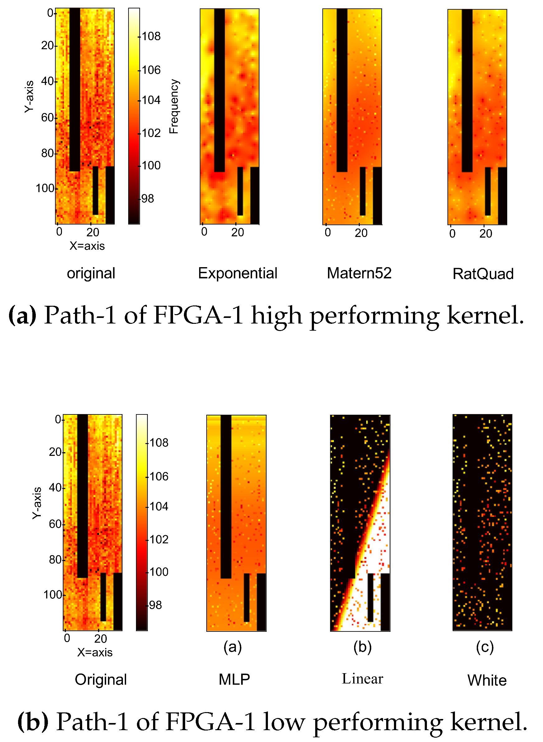
Figure 14.
Overall estimation error comparison of the best individual, hybrid, and adaptive kernels, and the proposed custom-adaptive kernel for FPGA and Wafer data.
Figure 14.
Overall estimation error comparison of the best individual, hybrid, and adaptive kernels, and the proposed custom-adaptive kernel for FPGA and Wafer data.

In the FPGA dataset, the analysis is also shown in Figure 14, the single best kernel slightly outperforms both the adaptive and hybrid kernels in baseline comparisons. Nevertheless, the Proposed custom adaptive kernel again demonstrates superior performance with the lowest FPGA error rate of 8.152, followed closely by the best kernel at 8.163 and the adaptive kernel with an error rate of 8.36. The hybrid kernel, however, exhibits notably higher FPGA error rates, indicating suboptimal performance for FPGA-based applications.
In the comprehensive analysis across both datasets, the Proposed custom adaptive-kernel kernel emerges as the most effective solution, consistently achieving superior performance. While the hybrid kernel demonstrates competitive accuracy in wafer-based applications, its significantly elevated FPGA error rate renders it unsuitable for universal deployment across both platforms.
The proposed adaptive kernel strategy introduces a modest overhead, primarily due to the one-time kernel selection and weight assignment step. Training time increases by approximately 1.3× to 1.5× compared to single-kernel GPR, while inference time remains nearly unchanged.
5. Conclusion
This study investigated the application of Gaussian Process Regression (GPR), a state-of-the-art technique, for wafer-level variation modeling and FPGA delay prediction, with an emphasis on kernel function selection. Through exhaustive analysis, various kernel functions, including hybrid and adaptive kernels, were evaluated using wafer-level industry production data and silicon measurements from FPGAs. While no single kernel function consistently excelled across all datasets, our proposed custom-adaptive kernel through a dynamic weighted-kernel approach demonstrated superior versatility and reliability. This novel methodology enhances the predictive performance and adaptability of GPR, addressing limitations in current state-of-the-art applications. Although the performance improvement in terms of average error may appear marginal on a per-dataset basis, the strength of the proposed custom-adaptive kernel lies in its robust generalization across structurally diverse datasets. Unlike single or static hybrid kernels, our approach dynamically adapts to the underlying data distribution by assigning data-driven weights to the top-performing kernels. This adaptability leads to consistent performance on both wafer-level and FPGA datasets each having distinct noise characteristics and spatial variance patterns demonstrating the model’s practical utility in semiconductor testing scenarios. By offering robust accuracy across diverse scenarios, this approach presents a practical and innovative solution for optimizing semiconductor testing and production processes, with the potential to significantly reduce costs and improve efficiency. These contributions represent a meaningful advancement in leveraging GPR for semiconductor manufacturing and related domains.
Riaz-ul-haque Mian received B.E. from Islamic University Bangladesh and M.E degree from Bangladesh University of Engineering and Technology (BUET) in 2009 and 2017 respectively. He received his Ph.D. degree from Graduate School of Information Science, Nara Institute of Science and Technology (NAIST), Japan in 2021. He was with Synesis IT Ltd. and GIZ from 2009 to 2017. Currently, he is an assistant professor of the Department of Information System Design and Data Science at Shimane University, Japan. His research interests include computer architecture, VLSI testing and decimal computing. He is a member of IEEE.
Foisal Ahmed (Member, IEEE) received his Bachelor of Engineering (B.E.) degree from Prime University, Dhaka, Bangladesh, in 2008. He completed his Postgraduate Diploma (P.G.D.) at the Bangladesh University of Engineering and Technology (BUET), Dhaka, in 2014, and his Master of Engineering (M.E.) degree at the Islamic University of Technology, Dhaka, in 2016. In 2020, he earned his Doctor of Philosophy (Ph.D.) degree from the Graduate School of Information Science at the Nara Institute of Science and Technology (NAIST), Nara, Japan. Previously, he served as a faculty member in the Department of Electrical and Electronic Engineering at Prime University, Bangladesh. He later worked as a postdoctoral researcher in the Department of Computer Systems at Tallinn University of Technology, Tallinn, Estonia. Currently, he is an Embedded Software Engineer at Stonridge Electronics, Inc., based in Estonia. His research interests encompass reliable embedded system design, fault-tolerant computing systems, counterfeit FPGA detection, hardware security and reliability, very-large-scale integration (VLSI) testing, the Internet of Things (IoT), and cyber-physical systems.
Hagihara Yoshito Currently pursuing B.E. degree from the Interdisciplinary Faculty of Science and Engineering, Department of Information System Design and Data Science at Shimane University, Japan. His research interests include VLSI testing.
Souma Yamane Received B.E. degree from the Interdisciplinary Faculty of Science and Engineering, Department of Information System Design and Data Science at Shimane University, Japan. He is currently pursuing her MS degree in the Smart Computing Lab, in the same department. His research interests include VLSI testing.
Data Availability Statement
This study utilized two datasets:
1. The FPGA dataset used in this study can be made available upon reasonable request from the corresponding author. Researchers requesting this dataset must provide a clear research purpose and will need to agree to terms of use.
2. The second dataset, which consists of industry production data, is subject to a non-disclosure agreement (NDA). Access to this dataset can be facilitated through direct communication with the industry contact, as provided by the corresponding author.
Funding Declaration
This research did not receive any specific grant from funding agencies in the public, commercial, or not-for-profit sectors.
Competing Interest Declaration
The authors declare that they have no competing interests.
Author Contributions
Riaz-ul-Haque Mian: Conceptualization, Methodology, Software, Visualization, Writing Original Draft Preparation, Project Administration
Foisal Ahmed: Data Curation, Review.
Yoshito Hagihara: Experiment, Writing
Yamane Souma: Validation, Formal Analysis.
All authors have read and approved the final manuscript.
References
- Ahmadi, A., Huang, K., Natarajan, S., Carulli, J.M., Makris, Y.: Spatio-temporal wafer-level correlation modeling with progressive sampling: A pathway to hvm yield estimation. In: 2014 International Test Conference, pp. 1–10 (2014).
- Ahmed, F., Shintani, M., Inoue, M.: Feature engineering for recycled FPGA detection based on wid variation modeling. In: 2019 IEEE European Test Symposium (ETS), pp. 1–2. IEEE (2019).
- Ahmed, F. , Shintani, M., Inoue, M.: Low cost recycled FPGA detection using virtual probe technique. In: 2019 IEEE International Test Conference in Asia (ITC-Asia), pp. 2019. [Google Scholar]
- Ahmed, F. , Shintani, M., Inoue, M.: Accurate recycled FPGA detection using an exhaustive-fingerprinting technique assisted by wid process variation modeling. 1626. [Google Scholar]
- Bahukudumbi, S., Chakrabarty, K.: Wafer-level testing and test during burn-in for integrated circuits. Artech House (2010).
- Bu, A. , Wang, R., Jia, S., Li, J.: Gpr-based framework for statistical analysis of gate delay under nbti and process variation effects. 1336. [Google Scholar]
- Candes, E.J. , Wakin, M.B.: An introduction to compressive sampling. 2008. [Google Scholar]
- Chang, C. , Chang, H.M., Chiang, K.: Study on gaussian process regression to predict reliability life of wafer level packaging with cluster analysis. In: 2022 17th International Microsystems, Packaging, Assembly and Circuits Technology Conference (IMPACT), pp. 2022. [Google Scholar]
- Chang, C. , Zeng, T.: A hybrid data-driven-physics-constrained gaussian process regression framework with deep kernel for uncertainty quantification. 1121. [Google Scholar]
- Dempster, A.P. , Laird, N.M., Rubin, D.B.: Maximum likelihood from incomplete data via the EM algorithm. Journal of the Royal Statistical Society. 1977. [Google Scholar]
- Duvenaud, D.K. , Lloyd, J.R., Grosse, R., Tenenbaum, J.B., Ghahramani, Z.: Structure discovery in nonparametric regression through compositional kernel search. In: International Conference on Machine Learning, pp. 1166–1174. 2013. [Google Scholar]
- Garrou, P. : Wafer level chip scale packaging (wl-csp): An overview. 2000. [Google Scholar]
- Gotkhindikar, K.R. , Daasch, W.R., Butler, K.M., Carulli, J., Nahar, A.: Die-level adaptive test: Real-time test reordering and elimination. In: 2011 IEEE International Test Conference, pp. 1–10. 2011. [Google Scholar]
- GPy: GPy: A Gaussian process framework in python. http://github. 2012.
- Kupp, N. , Huang, K., Carulli Jr., J.M., Makris, Y.: Spatial correlation modeling for probe test cost reduction in RF devices. In: Proceedings of IEEE/ACM International Conference on Computer-Aided Design, pp. 2012. [Google Scholar]
- Kupp, N. , Huang, K., Carulli Jr, J.M., Makris, Y.: Spatial correlation modeling for probe test cost reduction in rf devices. In: Proceedings of the International Conference on Computer-Aided Design, pp. 2012. [Google Scholar]
- Li, X. , Rutenbar, R.R., Blanton, R.D.: Virtual probe: A statistically optimal framework for minimum-cost silicon characterization of nanoscale integrated circuits. In: Proceedings of the 2009 International Conference on Computer-Aided Design, pp. 2009. [Google Scholar]
- Marinissen, E.J. , Singh, A., Glotter, D., Esposito, M., Carulli, J.M., Nahar, A., Butler, K.M., Appello, D., Portelli, C.: Adapting to adaptive testing. In: 2010 Design, Automation & Test in Europe Conference & Exhibition (DATE 2010), pp. 556–561. 2010. [Google Scholar]
- Nery, A.S. , Sena, A.C., Guedes, L.S.: Efficient pathfinding co-processors for FPGAs. In: 2017 International Symposium on Computer Architecture and High Performance Computing Workshops (SBAC-PADW), pp. 2017. [Google Scholar]
- Reda, S. , Nassif, S.R.: Accurate spatial estimation and decomposition techniques for variability characterization. 2010. [Google Scholar]
- Riaz-ul-haque, M. , Michihiro, S., Inoue, M.: Hardware–software co-design for decimal multiplication. 2021. [Google Scholar]
- Riaz-ul-haque, M. , NAKAMURA, T., KAJIYAMA, M., EIKI, M., SHINTANI, M.: Efficient wafer-level spatial variation modeling for multi-site rf ic testing. 1139. [Google Scholar]
- Riaz-ul-haque, M. , Shintani, M., Inoue, M.: Decimal multiplication using combination of software and hardware. In: Proceedings of IEEE Asia Pacific Conference on Circuits and Systems, pp. 2018. [Google Scholar]
- Riaz-ul-haque, M. , Shintani, M., Inoue, M.: Cycle-accurate evaluation of software-hardware co-design of decimal computation in RISC-V ecosystem. In: IEEE International System on Chip Conference, pp. 2019. [Google Scholar]
- Shintani, M. , Inoue, M., Nakamura, Y.: Artificial neural network based test escape screening using generative model. In: Proceedings of IEEE International Test Conference, p. 9. 2018. [Google Scholar]
- Shintani, M. , Mian, R., Inoue, M., Nakamura, T., Kajiyama, M., Eiki, M.: Wafer-level variation modeling for multi-site rf ic testing via hierarchical gaussian process. In: 2021 IEEE International Test Conference (ITC), pp. 2021. [Google Scholar]
- Shintani, M. , Uezono, T., Takahashi, T., Hatayama, K., Aikyo, T., Masu, K., Sato, T.: A variability-aware adaptive test flow for test quality improvement. 1056. [Google Scholar]
- Stratigopoulos, H.G. : Machine learning applications in IC testing. P: In, 2018. [Google Scholar]
- Suwandi, R.C. , Lin, Z., Sun, Y., Wang, Z., Cheng, L., Yin, F.: Gaussian process regression with grid spectral mixture kernel: Distributed learning for multidimensional data. In: 2022 25th International Conference on Information Fusion (FUSION), pp. 2022. [Google Scholar]
- Violante, M. , Sterpone, L., Manuzzato, A., Gerardin, S., Rech, P., Bagatin, M., Paccagnella, A., Andreani, C., Gorini, G., Pietropaolo, A., et al.: A new hardware/software platform and a new 1/e neutron source for soft error studies: Testing FPGAs at the isis facility. 1184. [Google Scholar]
- Wan, Z. , Yu, B., Li, T.Y., Tang, J., Zhu, Y., Wang, Y., Raychowdhury, A., Liu, S.: A survey of fpga-based robotic computing. 2021. [Google Scholar]
- Wang, L.C. : Experience of data analytics in EDA and test—principles, promises, and challenges. 2017. [Google Scholar]
- Xanthopoulos, C. , Huang, K., Ahmadi, A., Kupp, N., Carulli, J., Nahar, A., Orr, B., Pass, M., Makris, Y.: Gaussian Process-Based Wafer-Level Correlation Modeling and Its Applications, pp. 119–173. 2019. [Google Scholar]
- Yilmaz, E. , Ozev, S., Sinanoglu, O., Maxwell, P.: Adaptive testing: Conquering process variations. P: In, 2012. [Google Scholar]
- Zhang, S. , Lin, F., Hsu, C.K., Cheng, K.T., Wang, H.: Joint virtual probe: Joint exploration of multiple test items’ spatial patterns for efficient silicon characterization and test prediction. P: In, 2014. [Google Scholar]
- Zhang, W. , Li, X., Liu, F., Acar, E., Rutenbar, R.A., Blanton, R.D.: Virtual probe: A statistical framework for low-cost silicon characterization of nanoscale integrated circuits. 1814. [Google Scholar]
- Zhang, W. , Li, X., Rutenbar, R.A.: Bayesian virtual probe: Minimizing variation characterization cost for nanoscale IC technologies via Bayesian inference. In: Proceedings of ACM/EDAC/IEEE Design Automation Conference, pp. 2010. [Google Scholar]
Figure 1.
Comparison of heat maps for predictions by different methods for wafer data with 10% training data from industry measured values: (a) Original, (b) VP, (c) Gaussian Process Regression(GPR [14]).
Figure 1.
Comparison of heat maps for predictions by different methods for wafer data with 10% training data from industry measured values: (a) Original, (b) VP, (c) Gaussian Process Regression(GPR [14]).
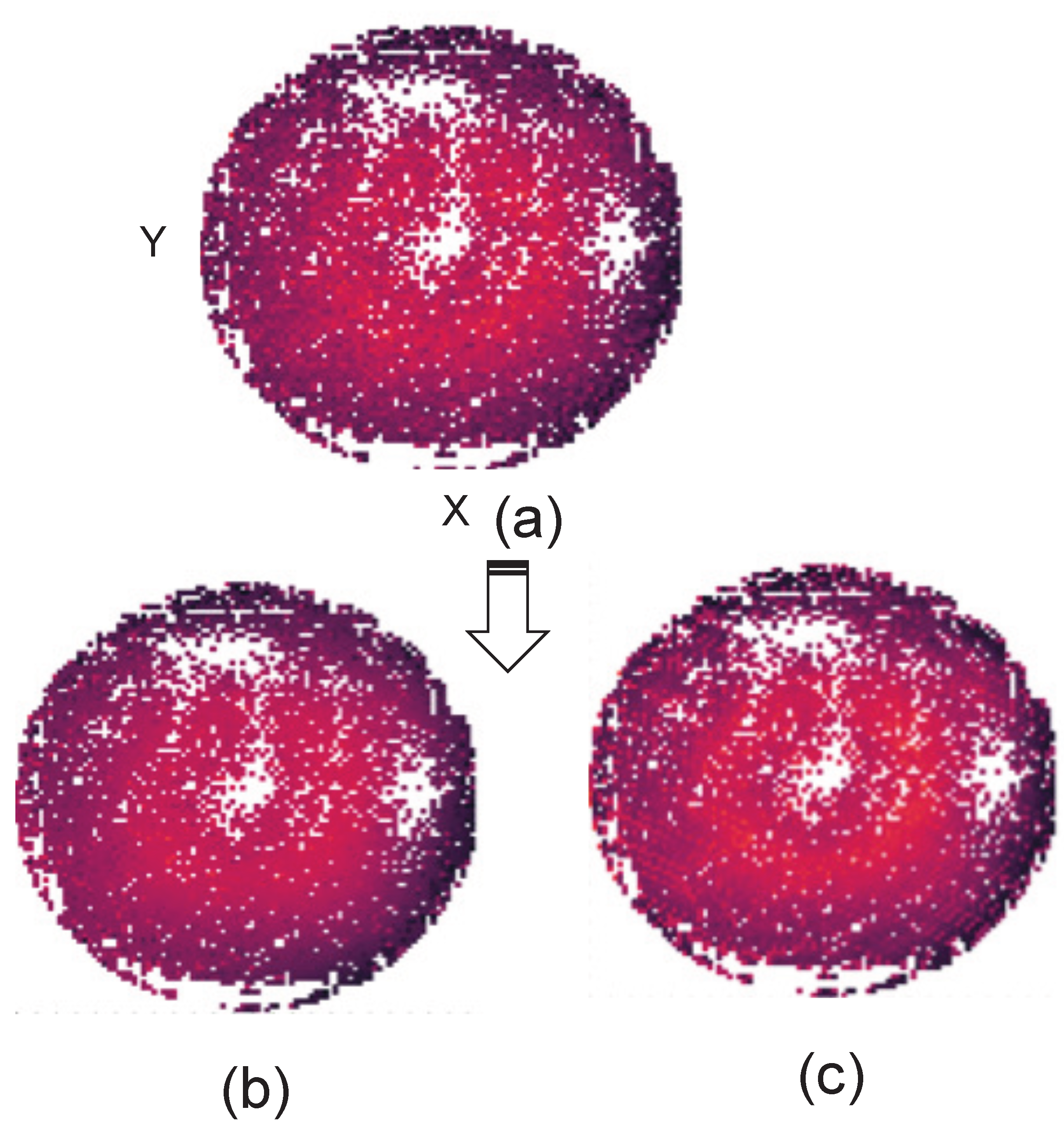
Figure 2.
Comparison of heat maps for predictions by different methods for FPGA delay measurement of ring oscillator using 10% training data: (a) Original, (b) VP, (c) Gaussian Process Regression (GPR [14]).
Figure 2.
Comparison of heat maps for predictions by different methods for FPGA delay measurement of ring oscillator using 10% training data: (a) Original, (b) VP, (c) Gaussian Process Regression (GPR [14]).
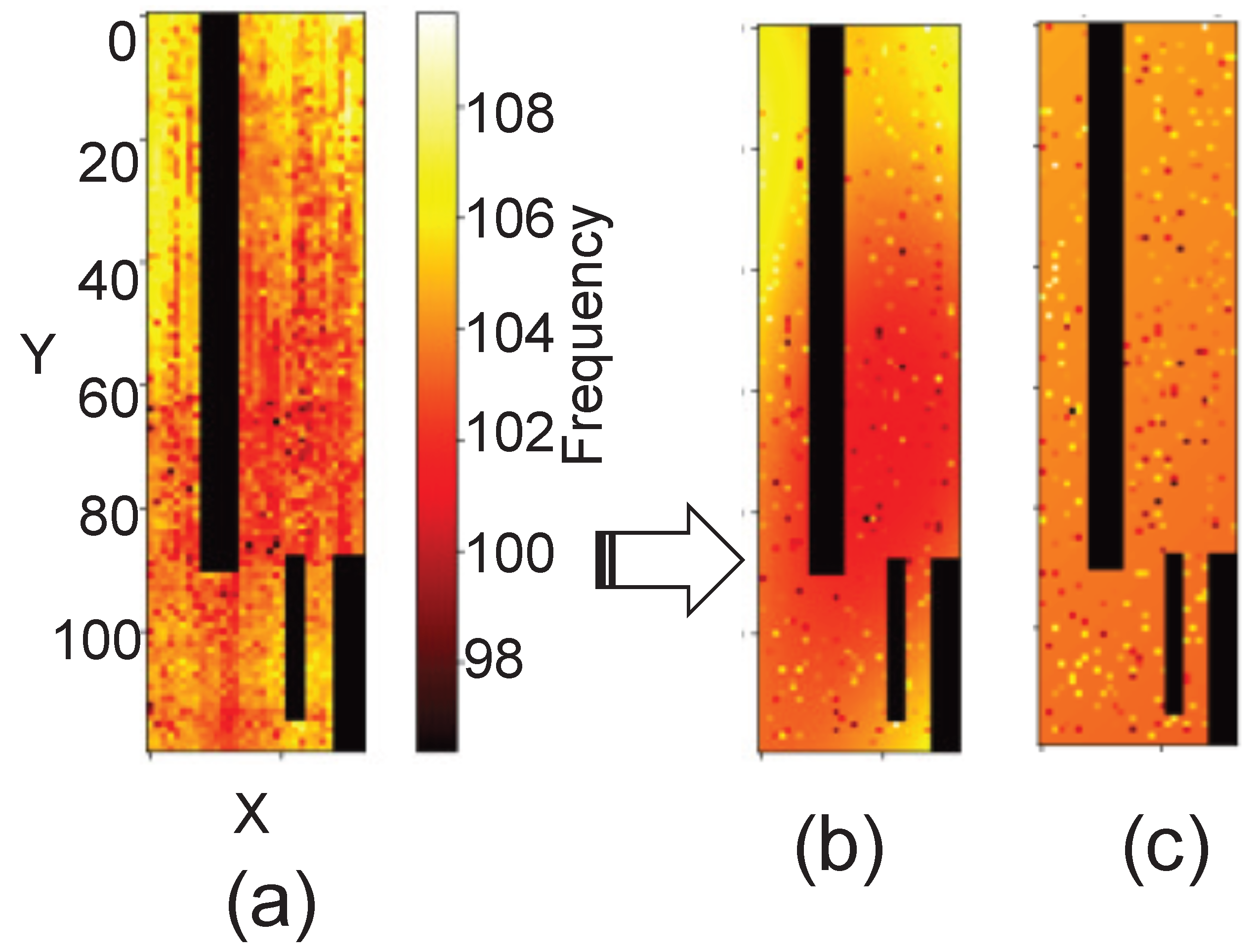
Figure 3.
Illustration of an FPGA wafer layout highlighting Configurable Logic Blocks (CLBs), Look-Up Tables (LUTs), scribe lines, Test Element Groups (TEGs), and flat zones.
Figure 3.
Illustration of an FPGA wafer layout highlighting Configurable Logic Blocks (CLBs), Look-Up Tables (LUTs), scribe lines, Test Element Groups (TEGs), and flat zones.
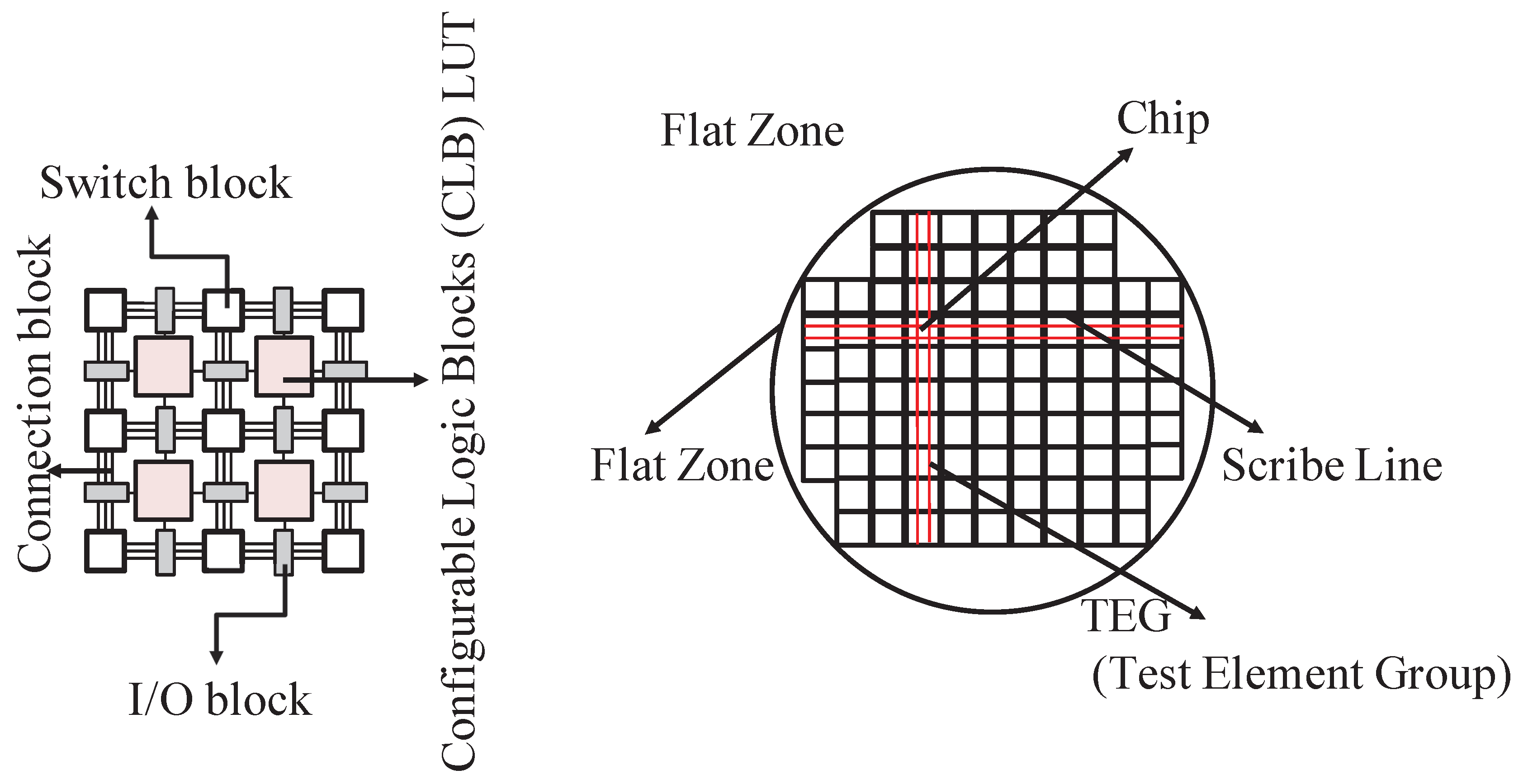
Figure 4.
Model of the kernel matrix derivation process.
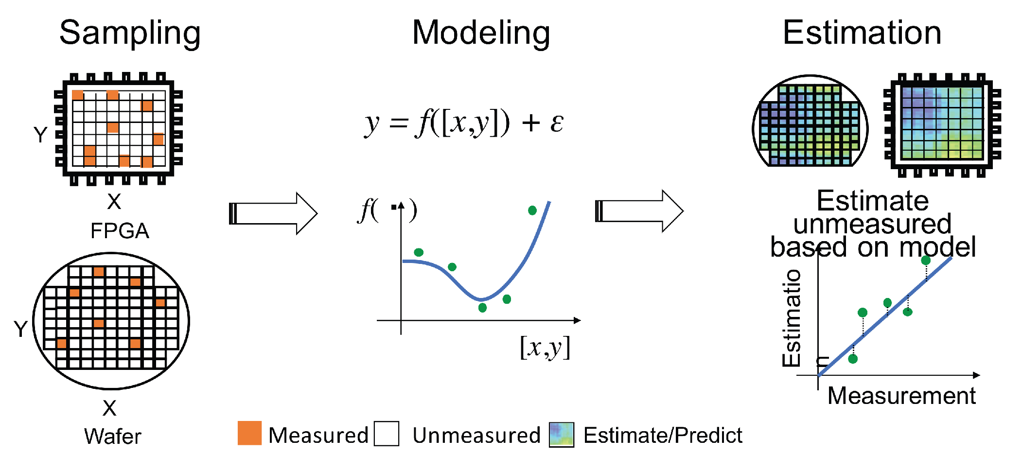
Figure 5.
Gaussian process regression model to predict Y from input X.
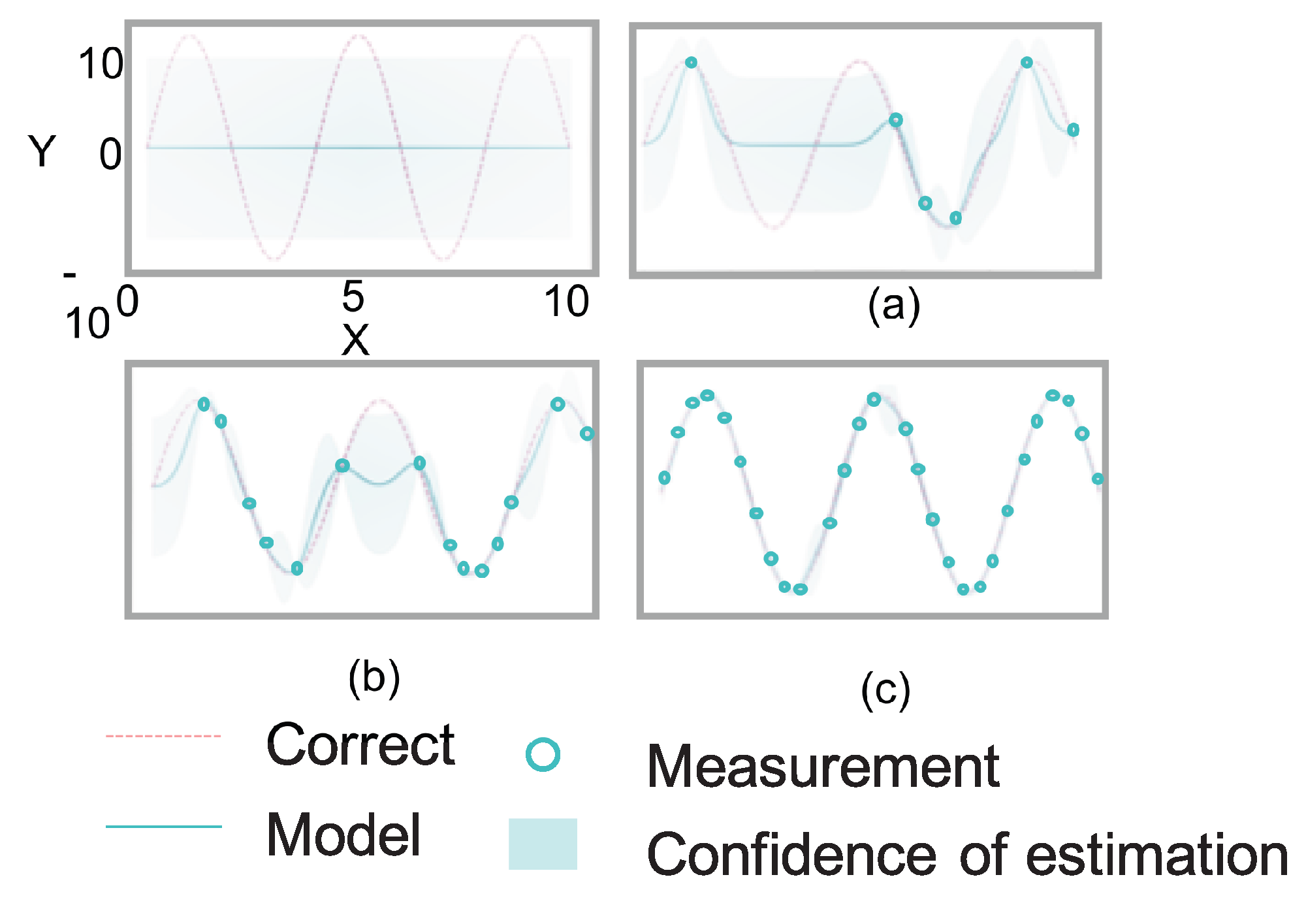
Figure 6.
Predictive variance vs. average error and cumulative error for Matern52 kernel.
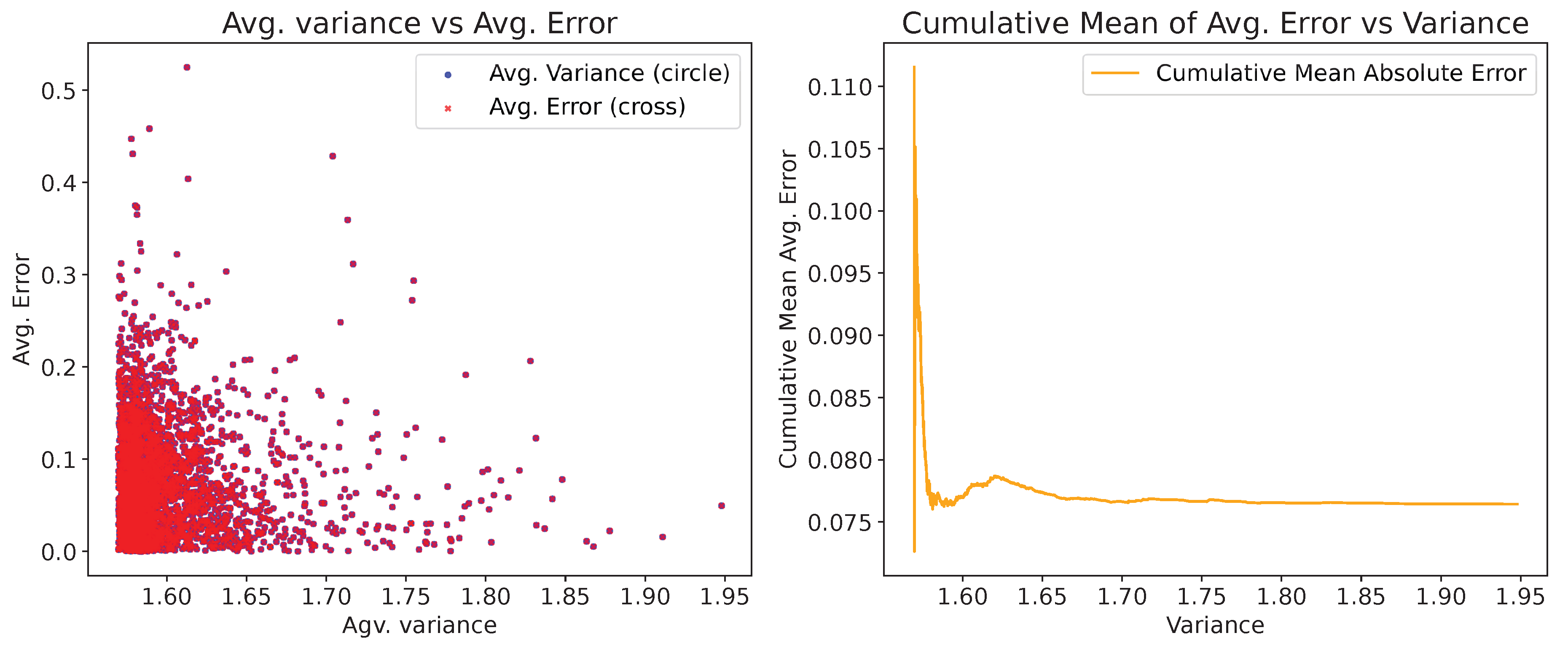
Figure 7.
Predictive variance vs. average error and cumulative error for Linear kernel.
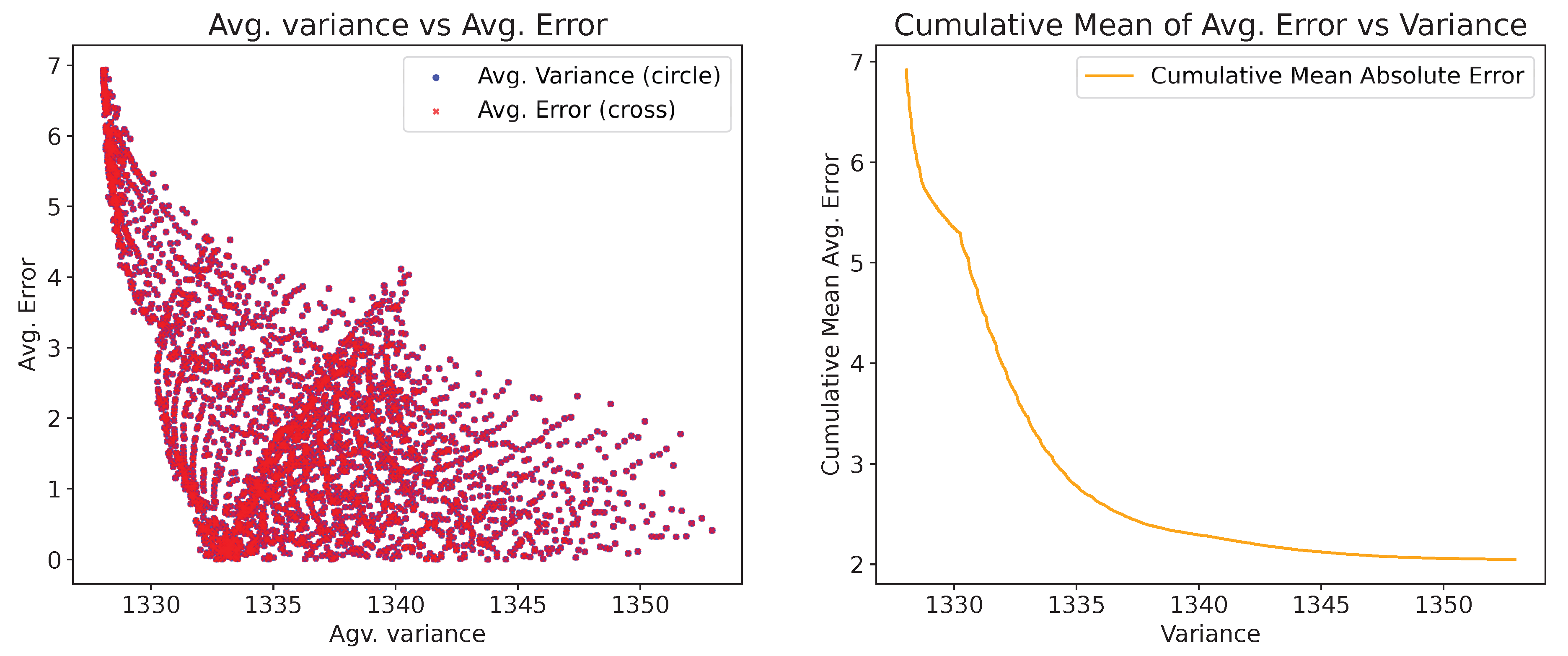
Figure 8.
Proposed adaptive kernel methodology.
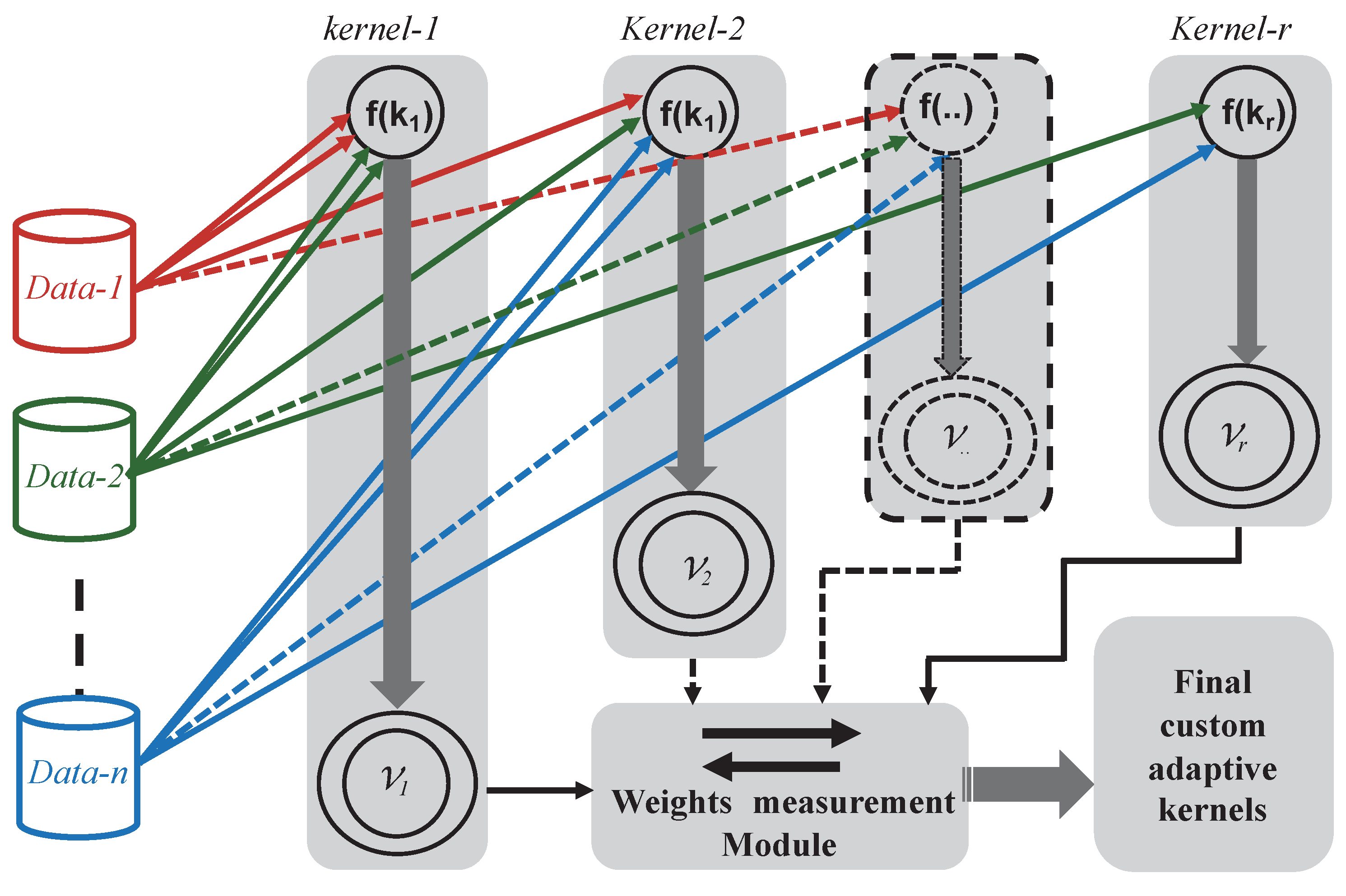
Figure 9.
Adaptive kernel generator module : relationship between , , and the variance difference , considering scaling factor .
Figure 9.
Adaptive kernel generator module : relationship between , , and the variance difference , considering scaling factor .
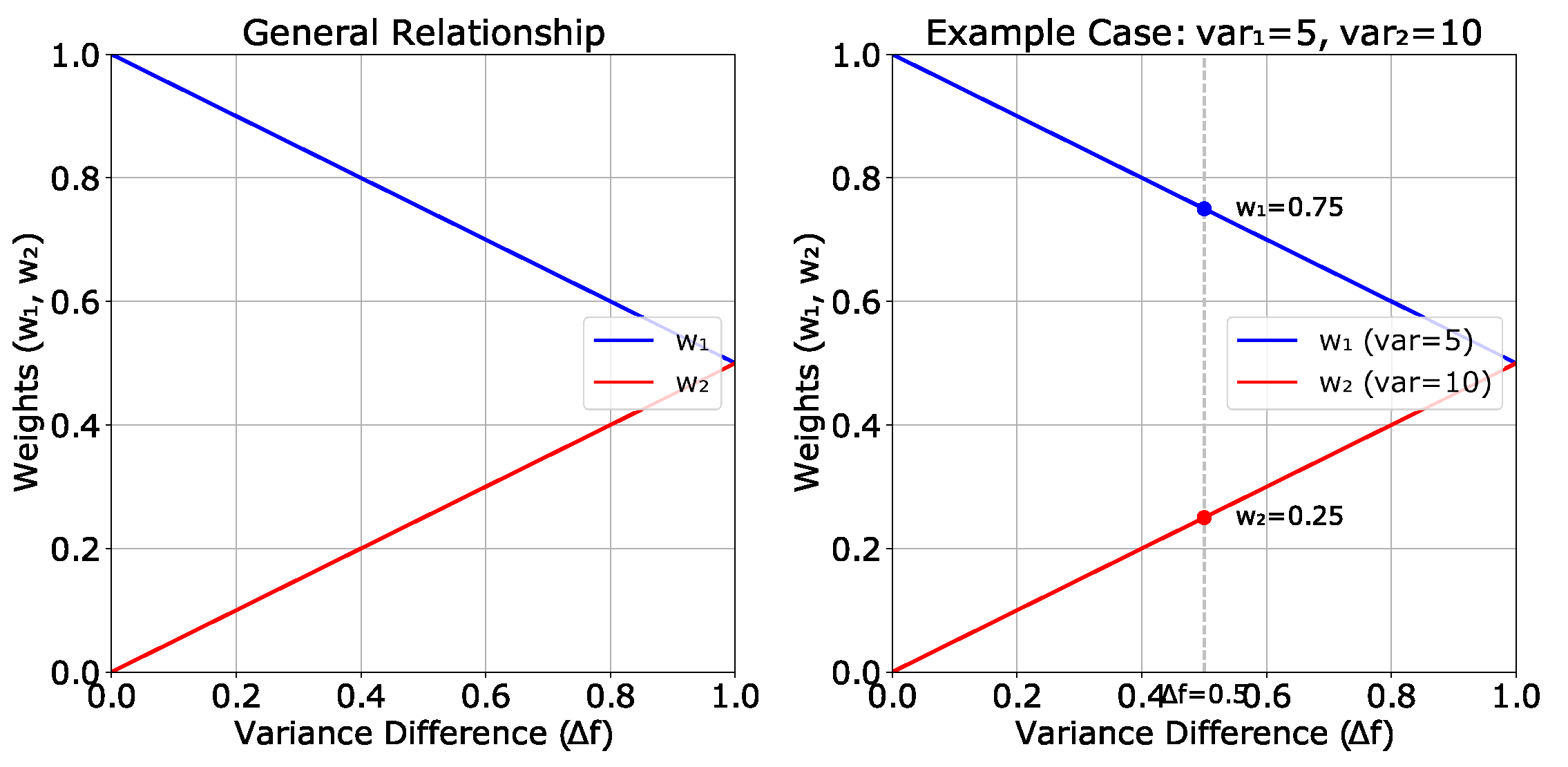
Figure 10.
Comparison of heat maps for the measured value between the original and other kernels.
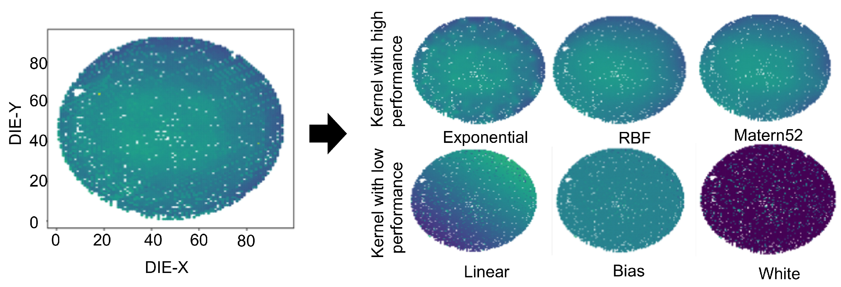
Figure 11.
Average estimation error () of the top four performing kernels for wafer data.
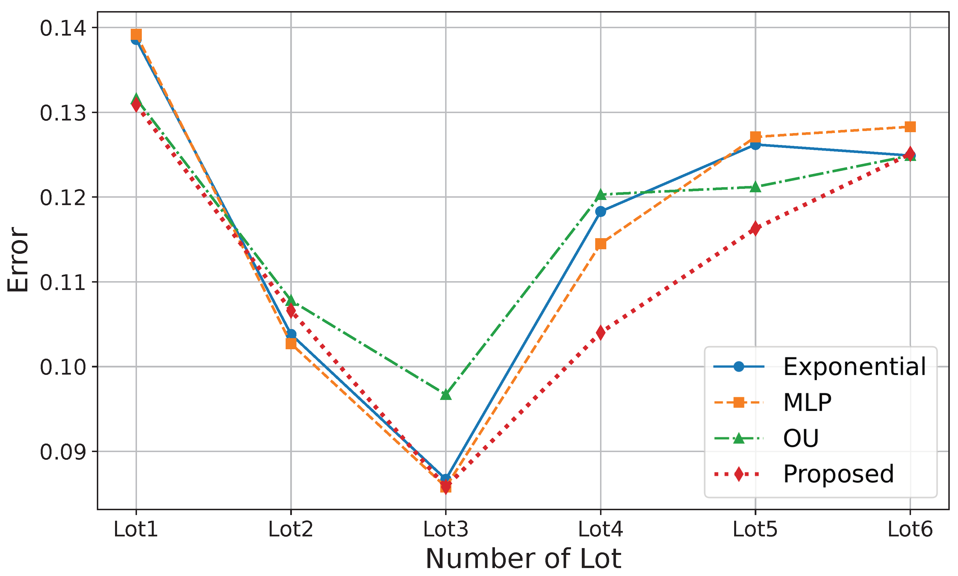
Figure 12.
Average estimation error () of the top four performing kernels for FPGA data.
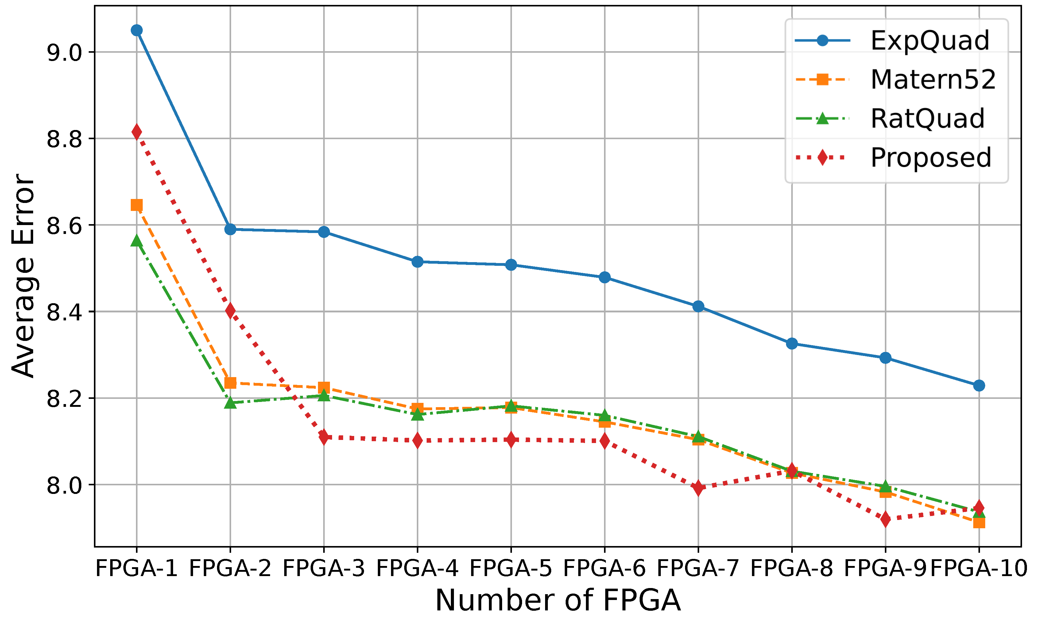

Table 1.
Kernel Selection Strategies for Wafer and FPGA Data
| Method | Wafer Kernels | FPGA Kernels |
|---|---|---|
| Hybrid | • MLP (Error: 0.116) | • RatQuad (Error: 8.154) |
| (Equal Weighted by top prediction Error) | • Exponential (Error: 0.117) | • Matern52 (Error: 8.163) |
| Adaptive | • MLP | • Matern52 |
| (Weighted by validation accuracy) | • Exponential | • RatQuad |
| • RBF | • Matern32 | |
| • OU | • Exponential | |
| Proposed | • Exponential + RBF | • Matern52 + Exponential |
| (Weighted by predictive variance) |
Table 2.
Average error () of different kernels for wafer data. The best-performing kernel (averaged per lot) is shown in bold.
Table 2.
Average error () of different kernels for wafer data. The best-performing kernel (averaged per lot) is shown in bold.
| Kernel | Lot1 | Lot2 | Lot3 | Lot4 | Lot5 | Lot6 | Average |
|---|---|---|---|---|---|---|---|
| Bias | 0.1708 | 0.1842 | 0.1471 | 0.1596 | 0.1726 | 0.1996 | 0.1726 |
| ExpQuad | 0.1395 | 0.1132 | 0.0881 | 0.1158 | 0.1293 | 0.1343 | 0.1203 |
| Linear | 0.2399 | 0.2709 | 0.2393 | 0.2082 | 0.2587 | 0.2538 | 0.2451 |
| Poly | 0.1392 | 0.1201 | 0.0908 | 0.1157 | 0.1318 | 0.1372 | 0.1227 |
| vRBF | 0.1395 | 0.1132 | 0.0881 | 0.1158 | 0.1293 | 0.1343 | 0.1203 |
| Exponential | 0.1386 | 0.1038 | 0.0867 | 0.1183 | 0.1262 | 0.1249 | 0.1166 |
| GridRBF | 0.1395 | 0.1132 | 0.0881 | 0.1158 | 0.1293 | 0.1343 | 0.1203 |
| Matern32 | 0.1397 | 0.1062 | 0.0862 | 0.1146 | 0.1282 | 0.1288 | 0.1175 |
| Matern52 | 0.1404 | 0.1066 | 0.0869 | 0.1152 | 0.1290 | 0.1310 | 0.1184 |
| MLP | 0.1392 | 0.1027 | 0.0858 | 0.1145 | 0.1271 | 0.1283 | 0.1163 |
| OU | 0.1316 | 0.1078 | 0.0967 | 0.1203 | 0.1212 | 0.1249 | 0.1266 |
| RatQuad | 0.1398 | 0.1133 | 0.0863 | 0.1146 | 0.1292 | 0.1347 | 0.1199 |
| StdPeriodic | 0.1706 | 0.1807 | 0.1417 | 0.1547 | 0.1724 | 0.1996 | 0.1703 |
| White | 0.6938 | 0.8575 | 0.7049 | 0.6113 | 0.7696 | 0.7569 | 0.7324 |
| Hybrid(MLP+Exponential) | 0.1359 | 0.1037 | 0.858 | 0.1140 | 0.1263 | 0.1251 | 0.1153 |
| Adaptive | 0.169 | 0.1227 | 0.088 | 0.1188 | 0.1433 | 0.1351 | 0.1295 |
| Proposed | 0.1309 | 0.1066 | 0.0858 | 0.1040 | 0.1163 | 0.1251 | 0.1115 |
Table 3.
Average error () of different kernels for FPGA data. The best-performing kernel (averaged per path) is shown in bold.
Table 3.
Average error () of different kernels for FPGA data. The best-performing kernel (averaged per path) is shown in bold.
| FPGA | FPGA-1 | FPGA-2 | FPGA-3 | FPGA-4 | FPGA-5 | FPGA-6 | FPGA-7 | FPGA-8 | FPGA-9 | FPGA-10 | AVG. |
|---|---|---|---|---|---|---|---|---|---|---|---|
| Bais | 10.570 | 9.993 | 9.882 | 9.711 | 9.790 | 9.912 | 9.886 | 9.875 | 9.916 | 9.809 | 9.934 |
| ExpQuad | 9.050 | 8.590 | 8.584 | 8.515 | 8.508 | 8.479 | 8.412 | 8.326 | 8.293 | 8.229 | 8.499 |
| Linear | 216.582 | 205.011 | 206.836 | 204.727 | 204.727 | 205.799 | 205.085 | 203.605 | 203.242 | 201.628 | 205.724 |
| vRBF | 9.050 | 8.590 | 8.584 | 8.515 | 8.508 | 8.479 | 8.412 | 8.326 | 8.293 | 8.229 | 8.499 |
| Exponential | 8.863 | 8.437 | 8.420 | 8.355 | 8.385 | 8.350 | 8.309 | 8.232 | 8.186 | 8.113 | 8.365 |
| GridRBF | 9.050 | 8.590 | 8.584 | 8.515 | 8.508 | 8.479 | 8.412 | 8.326 | 8.293 | 8.229 | 8.499 |
| Matern32 | 8.641 | 8.240 | 8.292 | 8.264 | 8.274 | 8.247 | 8.207 | 8.121 | 8.083 | 8.020 | 8.239 |
| Matern52 | 8.646 | 8.235 | 8.224 | 8.175 | 8.178 | 8.145 | 8.104 | 8.027 | 7.983 | 7.913 | 8.163 |
| MLP | 11.714 | 16.503 | 15.706 | 17.086 | 16.748 | 15.688 | 14.898 | 14.539 | 14.043 | 14.666 | 15.159 |
| OU | 8.863 | 8.437 | 8.420 | 8.355 | 8.385 | 8.350 | 8.309 | 8.232 | 8.186 | 8.113 | 8.365 |
| RatQuad | 8.564 | 8.189 | 8.206 | 8.162 | 8.182 | 8.160 | 8.111 | 8.031 | 7.996 | 7.937 | 8.154 |
| StdPeriodic | 9.445 | 8.859 | 8.859 | 8.740 | 8.684 | 8.811 | 8.771 | 8.847 | 8.894 | 8.797 | 8.871 |
| White | 736.712 | 701.328 | 708.574 | 701.542 | 705.214 | 705.443 | 700.765 | 695.283 | 693.278 | 688.258 | 703.640 |
| Hybrid | 8.58 | 8.14 | 8.45 | 8.95 | 8.14 | 8.38 | 8.71 | 8.98 | 8.57 | 8.221 | 8.522 |
| Adaptive | 9.015 | 8.802 | 8.800 | 8.710 | 8.134 | 8.006 | 8.001 | 8.042 | 8.030 | 8.099 | 8.363 |
| Proposed | 8.815 | 8.402 | 8.110 | 8.102 | 8.104 | 8.101 | 7.992 | 8.032 | 7.920 | 7.946 | 8.152 |
Disclaimer/Publisher’s Note: The statements, opinions and data contained in all publications are solely those of the individual author(s) and contributor(s) and not of MDPI and/or the editor(s). MDPI and/or the editor(s) disclaim responsibility for any injury to people or property resulting from any ideas, methods, instructions or products referred to in the content. |
© 2025 by the authors. Licensee MDPI, Basel, Switzerland. This article is an open access article distributed under the terms and conditions of the Creative Commons Attribution (CC BY) license (http://creativecommons.org/licenses/by/4.0/).
Copyright: This open access article is published under a Creative Commons CC BY 4.0 license, which permit the free download, distribution, and reuse, provided that the author and preprint are cited in any reuse.


