Submitted:
21 August 2025
Posted:
22 August 2025
Read the latest preprint version here
Abstract
2D Ising model is simple yet powerful model to describe ferromagnetism. In this project, the phase transition and critical behaviour of the 2D Ising model using metropolis algorithm was investigated. The magnetisation vs temperature graph for different lattice size L = 5, L= 10, L = 15, L=20, L=30, was analyzed and compared. The analysis demonstrated a trend where the critical point becomes more sharply defined on increasing lattice size. The obtained value of critical temperature from graph closely approximates to the theoretical value. Hence the simulation successfully demonstrated the phase transition of magnetic material from ordered to disordered state. The significance of Ising model further extends far beyond its application in understanding magnetism. This study provides a deeper understanding of phase transition and critical behaviour.
Keywords:
Phase transition
; Ising model
; Ferromagnetism
; Magnetization
1. Introduction
1.1. Phase Transition
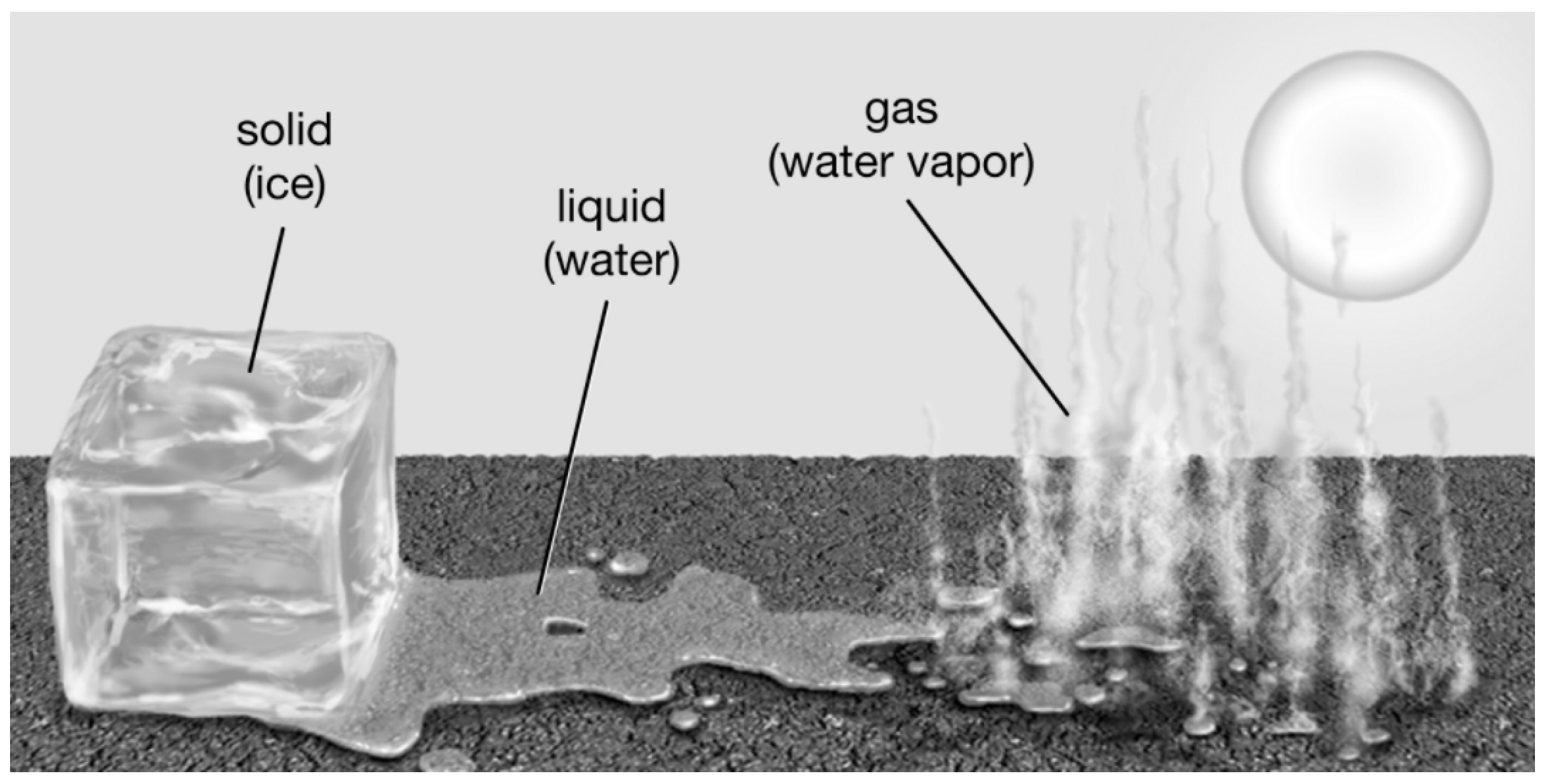
A phase transition occurs when the features of a system change abruptly and discontinuously. In other word, It is simply a change in the properties of a physical system that cause it to transit from one state to another. This occurs due to changes in external conditions such as temperature or pressure and are often accompanied by abrupt changes in properties like density, entropy, and volume. For instance,the transition of water from liquid to gas is an example of a phase transition, where the system changes its state due to variations in temperature and pressure.
Figure 1.
Phase transition [1].
Figure 1.
Phase transition [1].
The concept of phase transition is very significant in physics. These transitions are crucial for understanding a wide range of physical processes, from the formation of magnetic domains to critical behavior in materials. Phase transition are often associated with an order parameter because when any physical system changes it’s state,they often transit from orderliness to disorderliness or vice versa.
There are primarily two types of phase transition in thermodynamics. They are: First order and second order phase transition.
- First order phase transition: During first order phase transition, the system adsorbs or release latent heat. This heat is required to change the phase only without changing the temperature of system. Melting of ice, boiling of water falls in this category.
- Second Order phase transition: In this transition, no latent heat is involved and there is a continuous change of order parameter and near the transition point, the system exhibit critical behaviour. Ferromagnetic to paramagnetic transition is one of it’s example which we will discuss in this paper.
1.2. Ferromagnetism
Ferromagnetism is a property of certain metallic materials in which their atomic magnetic moments spontaneously align, even in the absence of an external magnetic field. Metals such as iron, cobalt, nickel etc are some of it’s example. The reason behind such a permanent magnetic moment is due to uncancelled electron spins. In this state material are said to be in order however above the room temperature, the regular order no more remains since the atomic magnetic moments orients randomly and substance becomes paramagnetic. The temperature above which the phase of magnetic material changes is known as critical temperature, . This temperature is also known as curie temperature.
Figure 2.
Second order phase transition [2].
Figure 2.
Second order phase transition [2].
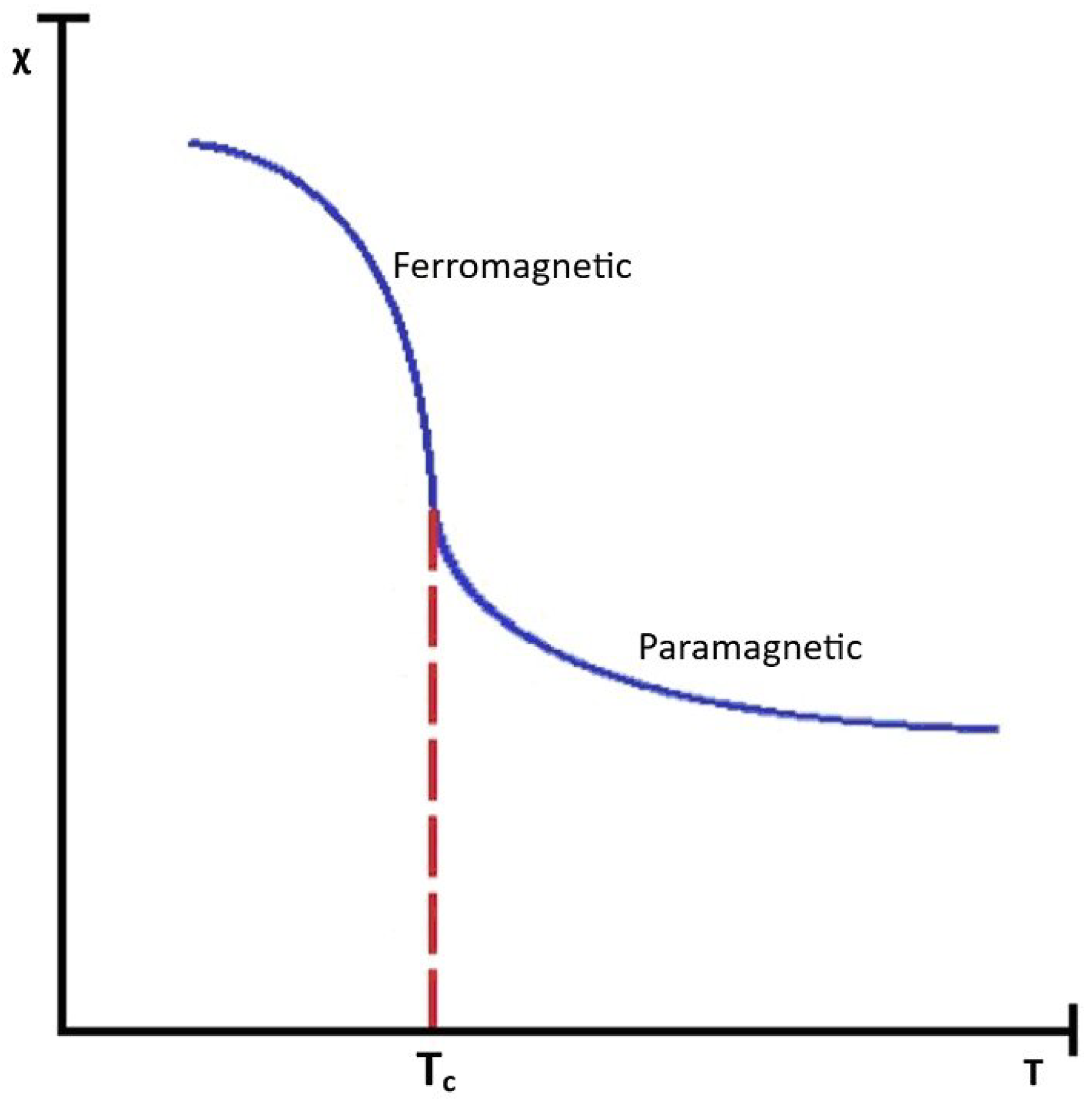
In other word transition of material from a paramagnetic state to a ferromagnetic state at critical temperature is known as phase transition. The system exhibits symmetry between up and down spins in paramagnetic state but as the temperature decreases the system transits to ferromagnetic phase. This is also known as spontaneous symmetry breaking as the system choose one of the two possible spin directions leading to net magnetization which disrupts the symmetry.
1.3. Ising model
Ising Model is a very important model that is especially used to describe ferromagnetism. It offers a simplified yet powerful way to understand phase transition which was invented by physicist Wilhelm Lenz in 1920 and his student Ernst Ising solved one dimensional Ising model in his thesis paper in 1924 [3]. Hence this model is often referred as “Ising model" or “Lenz-Ising model".
Figure 3.
The Ising model on a 2D square lattice [4].
Figure 3.
The Ising model on a 2D square lattice [4].
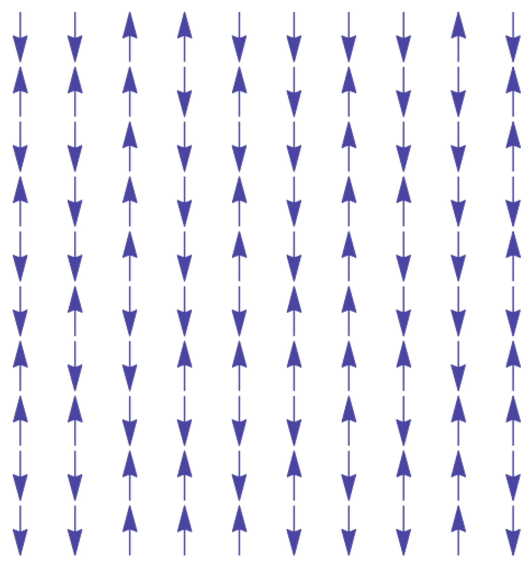
In this model, a system of magnetic particles can be modeled as a linear chain in one dimension or a lattice in two dimension, with one molecule or atom at each lattice site i [5]. Each atoms or molecule has a magnetic moment associated with it which is given by spin S, which can take only two possible values +1 or -1 based in their alignment. The behaviour of the Ising model changes drastically with dimensions. As mentioned above Ernst Ising solved Ising model in one dimension. Such system can be visualized as a linear chain of spins where each spin interacts with its immediate neighbours. Based on his findings, he concluded that the one dimension magnetic system exhibits no phase transition [6].
The Ising model undergoes a phase transition between an ordered and a disordered state in higher dimensions [3] which was verified by a physicist Rudolf Peierls back in 1936. Kramers and Wannier predicted the model’s critical temperature. However it wasn’t until 1944 where this model was solved analytically by Lars Onsager for two dimensional square lattice in absence of magnetic field. This work was groundbreaking as it provided an analytical expression for critical temperature. Onsager’s solution didnot explicitly quantify this critical point, Huang, K. (2008) determined the critical temperature to be in 2D Ising model [7] which is given by,
In this paper we will simulate the 2D Ising model for comparative analyzing the phase transition of given lattice sizes and eventually determined the critical temperature .
1.4. Theory
1.4.1. Lattice and Spin Configuration
In the Ising model, the lattice is a discrete grid of sites also known as nodes or vertices which are arranged in a particular geometric pattern. This can be in one dimension, two dimension or three dimension. Each lattice site k, where is the set of lattice sites, has a spin variable which can take one of the two values,
A spin configuration for the Ising model is given by, .
1.4.2. Hamiltonian of Ising Model
As the spins interact with their adjacent neighbours, the strength of their interaction at sites i and j is denoted by . If external magnetic field is also applied on a site j then the total energy of spin configuration S is given by,
Here the notation represents nearest-neighbour interaction and implies magnetic moment.
In the absence of external magnetic field i.e h=0 for all j in the lattice , then the Equation (6) becomes,
Similarly if we assume the interaction strength between all nearest neighbours is same i.e, = J. Then Equation (6) can further be simplified as,
Here, J>0 is the strength of exchange interaction.
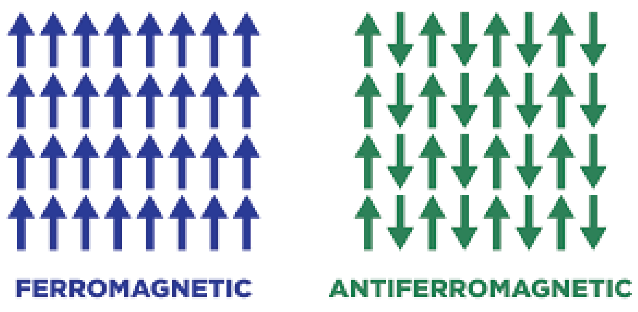
In above Hamiltonian, if 0 then the spins align with each other and makes the material ferromagnetic. Similarly, if 0 then the spins align in opposite direction making the material anti-ferromagnetic.
Figure 4.
Ferromagnetism and anti-ferromagnetism
The probability of the system being in a particular configuration S is used to determine by Boltzmann distribution. This probability is a critical concept that helps to understand how likely a particular arrangement of spins in a lattice is, in certain temperature. This function actually depends upon the Hamiltonian H and temperature of the system,
- is the inverse temperature.
- = Boltzmann constant.
- T = absolute temperature.
- = The partition function which ensures total probability across all configurations sums to one.
Basically, The system’s energy comes from the interaction of spins with one another and with the external magnetic field B. As electron spin and magnetic moment are comparable, we can consider a "dipole-dipole" interaction equivalent to a "spin-spin" interaction [8]. If each dipole is assumed to interacts with B and with nearest neighbour then the potential energy term is
Here, g is the gyro magnetic ratio.
is the Bohr magneton, which is a unit of magnetic moments.
1.5. Objectives
1.5.1. General Objectives
The main objective of the project work is to investigate and explain behaviour of phase transitions in ferromagnetic material, focusing on the 2D Ising model using Metropolis algorithm.
1.5.2. Specific Objectives
- To simulate the 2D Ising model and analyze the system’s behaviour at various temperature.
- To plot graph between magnetization and temperature of the magnetic lattice simulated in ising model.
- To determine the critical temperature through the graph plot.
2. Literature Review
Ising model is a well developed and simple model which can be used to explain the thermal behaviour and phase transition of ferromagnetic material. There are numerous researches conducted in past few decade to study the phase transition in 2D Ising model using various methods. The most popular one is Monte Carlo simulation.
[9] demonstrated Monte carlo simulation to simulate the 2D Ising model and explained the behaviour of the total energy and magnetization for a 40 ×40 lattice size. In their simulation, they found a phase transition at a critical temperature .
[10] have published a research using metropolis algorithm to determine curie temperature . In this article, the author simulated a 2D square lattice and utilized the metropolis algorithm to update the average energy per spin, average magnetisation per spin, specific heat capacity, and magnetic susceptibility, all of which were shown as functions of temperature. The curie temperature thus calculated was = 2.269 J/.
[11] have demonstrated detailed simulations of the 2D Ising model using metropolis algorithm, a type of Markov chain Monte Carlo method. Author studied the variation of magnetization and heat capacity with temperature for different lattice size and magnetic field. The estimated the critical temperature of an infinite 2D lattice was found to be 2.263±0.013 .
Similarly, [12] studied the Ising model from both theoretical and simulation perspective. In this research author have focused on studying the phase transiton using probabilistic language. In addition, 2D Ising model was also simulated through metropolis algorithm utilizing MATLAB. The obtained result of simulation were found to be compatible with a critical value ) as predicted by Onsager’s solution.
Many other advanced methods have been employed for studying the phase transition in 2D ferromagnetic Ising model[13]. have leveraged the application of deep learning autoencoders to investigate phase transition for different lattice sizes L to determine . Authors have calculated for each lattice sizes such as L= 25, 35, 50, 100, 150. Then, They have extrapolated these values to estimate the critical temperature for an infinitely large lattice by fitting data and found that = 2.266, which is very close to the exact critical temperature = 2.26918.
[14] studied phase transition in 2D and 3D Ising model using Markov chain Monte Carlo technique for a small lattice size and . The critical point for 2D Ising model has been determined to be at around 2.2 when no magnetic field was applied.This research has found that even in case of small lattice size L = 3, phase transition seems to exit.
2.1. Motivation
The 2D Ising model is very simple mathematical tool that can be used to study phase transition and critical phenomena in ferromagnetic material. Despite being simple, it captures essential physics behind many complex behaviours. From the literature reviews, It is evident that the numerous studies exists for the study of phase transition in 2D Ising model using various simulation methods from simple Monte Carlo to complex neural networks. Yet studying 2D Ising model using metropolis algorithm is simple but accurate algorithm in simulating phase transition in 2D Ising model for different lattice sizes. I am particularly motivated to analyze and compare phase transition and critical phenomena as the lattice size grows. Further, better understanding of phase transition in ferromagnets has wide applications not only in statistical mechanics and condensed matter physics but also in machine learning, Quantum computing and many emerging technologies.
3. Methodology
3.1. 2D Ising Model
In statistical mechanics, the two-dimensional square lattice Ising model is a simple lattice model of interacting magnetic spins [3]. It is noted for having non-trivial interactions but providing an analytical solution. Lars Onsager solved the model for the rare case where the external magnetic field H = 0. It is also one of the most simple statistical models to demonstrate a phase transition. [15].
3.2. Metropolis Algorithm
We use Monte Carlo simulation in order to simulation the phase transition of different lattice size in 2D Ising model.Monte Carlo simulations excels at studying phase transitions by allowing us to explore the system’s behavior at different temperatures. It is a computational method that uses random sampling to solve problems. It is extensively used in three major problem classes [16] : optimization, numerical integration and sampling from a probability distribution.
In this project, a finite two dimensional square lattice of atoms is considered where the lattice size of L× L is used. L takes the value of 5,10,15, 20,and 30 where each site has the spin +1 or -1. The Metropolis algorithm was used to implement the Ising Model on 2D lattices of varying sizes and the energy, absolute magnetisation and susceptibility per spin were plotted as a function of temperature. The Metropolis-Hastings algorithm is a Markov chain Monte Carlo (MCMC) approach that uses a probability distribution to generate a sequence of random samples(Wikipedia contributors, 2024b). In Monte Carlo simulations, we typically calculate the energy of the system for each configuration generated during the simulation. We then use these energies to estimate the expectation value of the energy [17]. In Monte Carlo simulations, we typically calculate the energy of the system for each configuration generated during the simulation. We then use these energies to estimate the expectation value of the energy. This value is essential for calculating other thermodynamic quantities like specific heat and magnetization. However, in this project we are only focusing on simulating the model for studying a phase transition from a ferromagnetic to a paramagnetic state through magnetization vs temperature graph of different lattice size. For this we have the average magnetization given by
where, N is the total number of sites.
Magnetization serves as an order parameter,distinguishing between the ferromagnetic and paramagnetic phases. In the ferromagnetic phase, the system exhibits a spontaneous net magnetization (M ≠ 0), in the absence of external magnetic field. In paramagnetic phase, the magnetization is zero on average (M = 0). Finally, we estimate critical temperature by looking at the graph since the average magnetization abruptly drops to zero as the temperature is increased through .
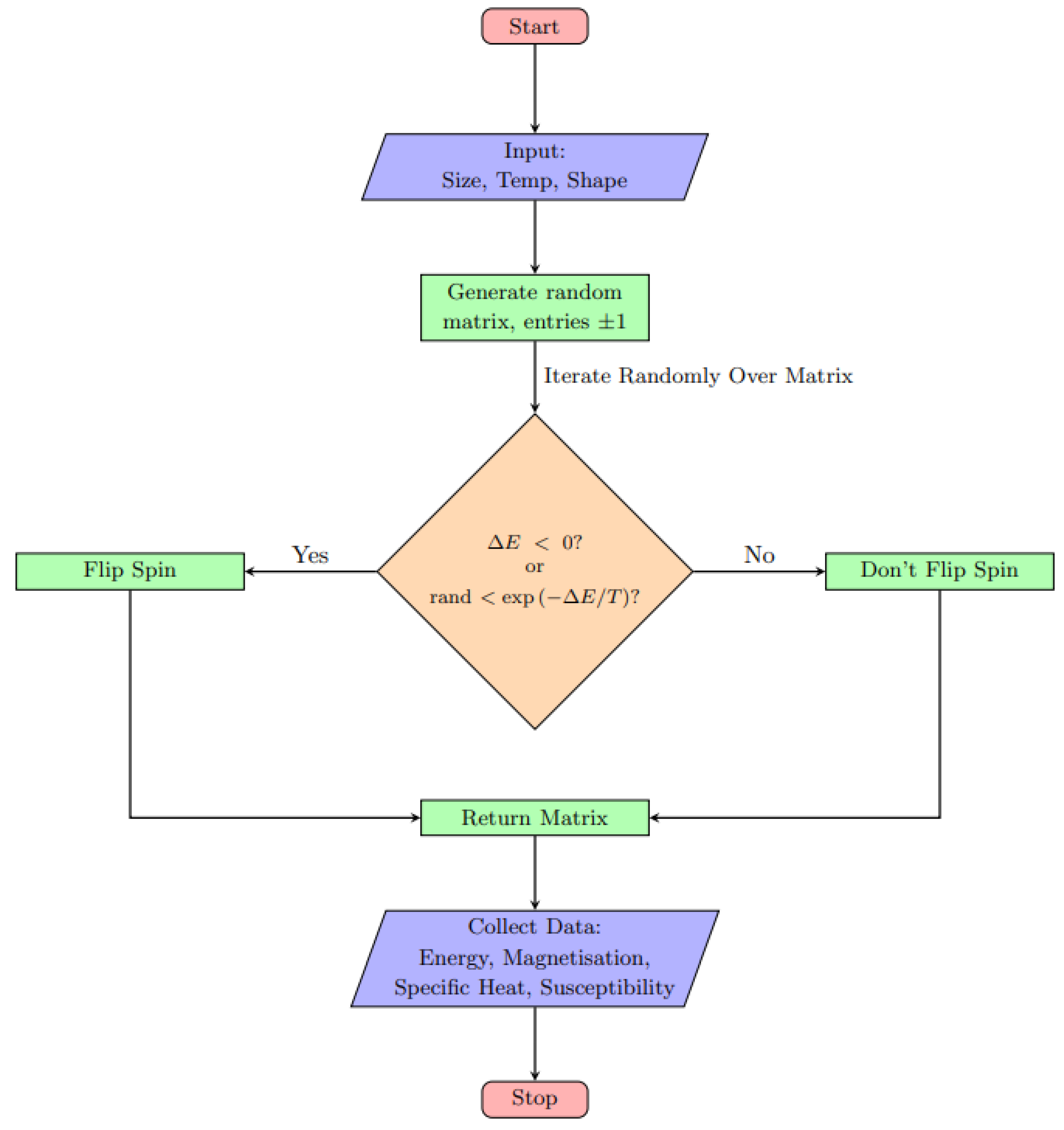
3.2.1. Steps of Metropolis algorithm
Metropolis algorithm was originally invented by Metropolis, Rosenbluth, Teller, and Teller in their simulation of neutron transmission by improving the Monte-Carlo simulation for averages in 1953 [8]. Python is used to simulate 2D Ising model using Metropolis algorithm for different lattice sizes for analyzing their critical behaviour.
The following are the steps to follow while simulating the Ising model in 2D using the Metropolis algorithm.
- Initialization: Firstly, we generate a random arbitrary spin configuration with energy .
- Spin Flip Process: We flip the spin of a lattice site selected at random. For instance, if spin was +1, alter it into -1, and vice versa and Calculate the energy using equation
- Change in Energy Calculation: Calculate the difference in energy generated by spin flip, = - and associated transition probability P = .
-
Acceptance Criteria: We then decide whether to accept the new configuration based on energy change.
- If 0 , then we accept the spin flip because it lowers the energy.
- We accept new state with probability P = , If .
- Calculation: Now we update the thermodynamics quantities such as average energy, magnetization, etc.
- Equilibrium Reached: Finally, we repeat the steps 2-6 with chosen spin configuration until thermal equilibrium is reached.
Figure 5.
A Flow chart of one sweep of metropolis algorithm [10].
Figure 5.
A Flow chart of one sweep of metropolis algorithm [10].
4. Results and Discussion
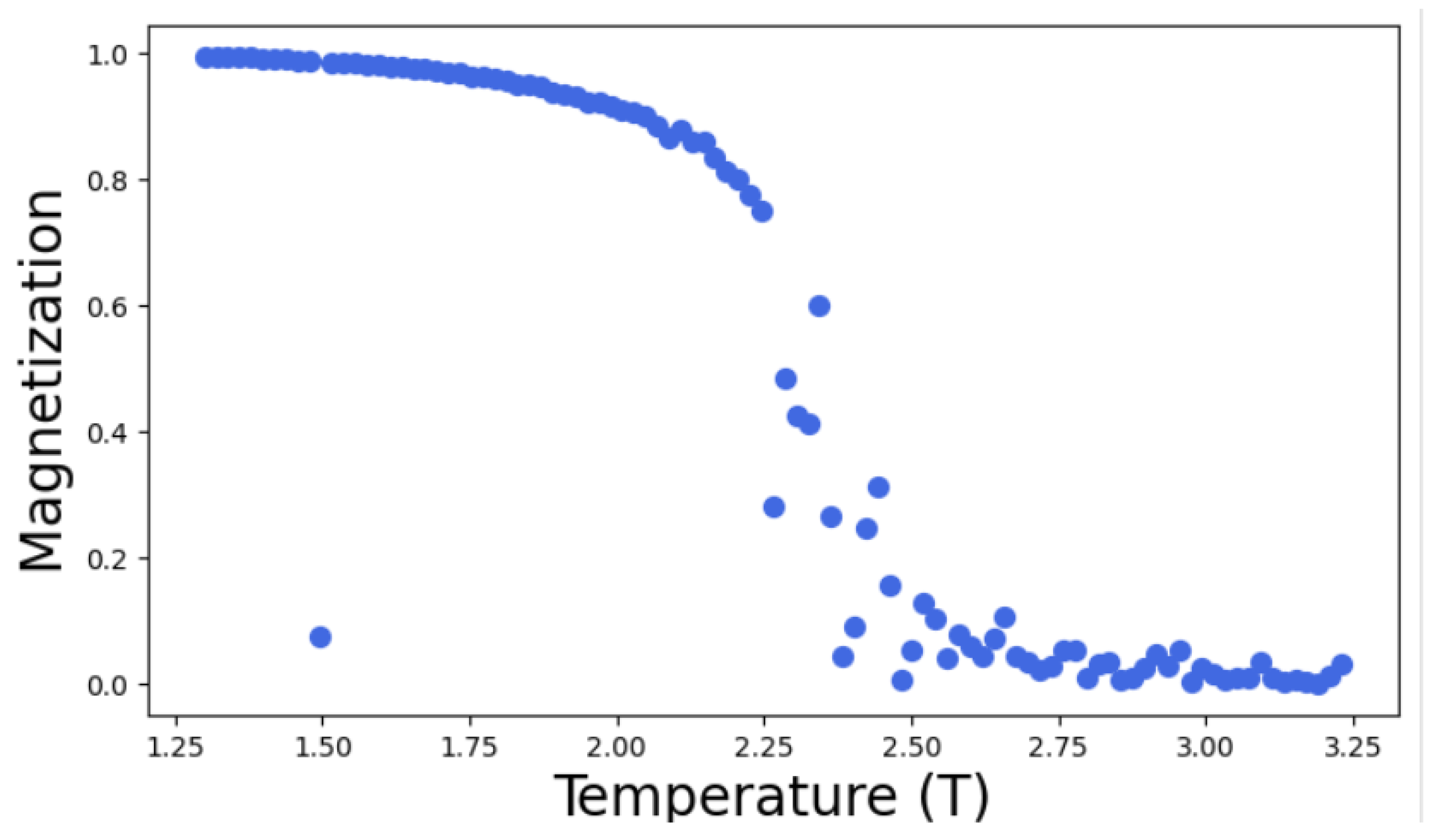
For the study of phase transition in 2D Ising model, Monte Carlo simulations were conducted with Monte-Carlo move(MC) = 1000 times using Metropolis algorithm for different lattice size L= 5,10,15,20,30. The resulting graph of magnetization is obtained as a function of temperature as follows;
From the analysis of the above graph, it becomes evident that as the lattice size increases in 2D Ising model the critical point becomes more sharply defined. This means that as the lattice grows, the critical point obtained is nearer and nearer to the theoretical value. In the above graph, the sudden disruption in the curve of Magnetization vs Temperature becomes more precise with increasing lattice size. This sudden drop of magnetization as a function of temperature in the given plots represents the transition from ordered to disordered state. This is because in the 2D Ising model, each lattice site has a spin that can be either up (+1) or down(-1). The system usually favours a state of minimum energy which can be achieved when most spins aligns but as the temperature increase, ordered spin configuration disrupts due to thermal agitation. As a result system tends towards disordered state with random spin orientations and hence the net magnetization decreases. In this way, the system changes from one state of high magnetization to low magnetization.
The point at which phase transition takes place is known as critical point or critical temperature . From the Figure 6, Figure 7, Figure 8, Figure 9 and Figure 10, as the lattice size increases critical point becomes more defined and hence the point at which phase transition occurs can approximated to be ≈ 2.26 J/, which nearly agrees with the theoretical value = 2.269185 [18] calculated for two dimensional square lattice of atoms. This results also agrees with the study conducted by [13] using auto-encoders, where author have stated that as the lattice size increases the phase transition occurs very close to exact critical temperature . Below the critical temperature , material is in ferromagnetic state and above , it’s phase changes into paramagnetic state. The slight discrepancy is due to the finite size effect as I have only considered lattice size of L= 5,L= 10,L=15 L= 20, L= 30 in the Ising model simulations. Finite-size effects in many-particle systems can significantly impact the accuracy of thermodynamic calculations in computer simulations [19].
5. Conclusions and Future Work
5.1. Conclusions
In this project, the phase transition behaviour of the 2D Ising model has been investigated for varying lattice sizes by Monte Carlo simulations particularly utilizing Metropolis algorithm. The result of the simulation is obtained in the form of Magnetization vs Temperature graph for each lattice size. The trend of curve in the simulated graph clearly indicates that on increasing the size of lattice L= 5,10,15, 20, 30, the critical point becomes sharper. This result aligns with the theoretical prediction and the approximated critical temperature is very close to the theoretical value. In addition the graph shows how magnetization in a material changes as temperature is increased. Hence the overall results strongly agrees with the significance of Ising model in capturing the physics behind the phase transition and critical behaviour of magnetic material.
5.2. Future Work
The metropolis algorithm employed in this research serves as powerful and popularly used method for simulating 2D Ising model but it does have many limitations. This algorithm is inefficient near critical temperature thus leading to longer simulation time. Even simulating the lattice size above 30 for 1000 Monte Carlo sweeps takes significant amount of time.
This research includes the simulation of only few lattice sizes, in future this work can be extended to investigate more powerful techniques like machine learning for simulating 2D Ising model for larger lattice size. Additionally, due to time constraints I have only analyzed the order parameter i.e magnetization with increasing temperature. Exploring the other thermodynamical quantities such as specific heat and susceptibility can provide deeper insights about the critical point. Although numerous researches has been done in Ising model, but only few researches have studied higher dimensional Ising models. This research serves as a benchmark for future studies to explore how dimensionality affects critical behaviour.
Appendix A
| Code for simulation of 2D Ising model for different lattice size L. I have taken L = 5, L= 10, L = 15, L=20, L=30 separately. |
| import numpy as np |
| from numpy.random import rand |
| import matplotlib.pyplot as plt |
| from_future_import division |
| def initialstate(L): |
| # random spin configuration generation for initial condition |
| state= 2*np.random.randint(2, size = (L,L)) - 1 |
| return state |
| def mcmove(config, beta): |
| #monte carlo (mc) move using metropolis algorithm |
| for i in range(L): |
| for j in range(L): |
| a = np.random.randint(0,L) |
| b = np.random.randint(0,L) |
| s = config[a,b] |
| nb = config[(a+1)%L,b] + config[a,(b+1)%L] + config[(a-1)%L,b] + config[a,(b-1)%L] |
| cost = 2*s*nb |
| if cost <0: |
| s*=-1 |
| elif rand() < np.exp(-cost*beta): |
| s*=-1 |
| config[a,b] = s |
| return config |
| def calcEnergy(config): |
| # Energy of given configuration |
| energy = 0 |
| for i in range(len(config)): |
| for j in range (len(config)): |
| S = config[i,j] nb = config[(i+1)%L,j]+config[i,(j+1)%L] + config[(i-1]%L,j] + config[i,(j-1)%L] |
| energy += -nb*S |
| return energy/4. |
| def calcMag(config): |
| # Magnetization of given configuration |
| mag = np.sum(config) |
| return mag |
| #parameters |
| nt = 99 # number of temperature points |
| L = 5 # size of the lattice, L x L |
| eqSteps = 1000 # number of MC sweeps for equilibrium |
| mcSteps = 1000 # number of MC sweeps for calculation |
| T = np.linspace(1.3,3.23,nt); |
| E,M = np.zeros(nt),np.zeros(nt) |
| n1,n2 = 1.0/(mcSteps*L*L), 1.0/(mcSteps*mcSteps*L*L) |
| for tt in range(nt): |
| E1 = M1 = E2 = M2 = 0 |
| config =initialstate(L) |
| iT = 1.0/T[tt]; iT2= iT*iT; |
| for i in range (eqSteps): |
| mcmove(config,iT) #montecarlo moves |
| for i in range(mcSteps): |
| mcmove(config,iT) |
| Energy = calcEnergy(config) |
| Mag = calcMag(config) |
| E1 = E1 + Energy |
| M1 = M1 + Mag |
| M2 = M2 + Mag*Mag |
| E2 = E2 + Energy*Energy |
| f = plt.figure(figsize=(18,10)); #plotting the values calculated |
| sp = f.add_subplot(2,2,2): |
| plt.scatter(T, abs(M), s=50,marker= ’o’,color=’RoyalBlue’) |
| plt.xlabel("Temperature(T)", fontsize=20); |
| plt.ylabel("Magnetization",fontsize = 20); plt.axis(’tight’) |
References
- Encyclopædia Britannica. States of Matter.
- Bailey, M. Domestic Applicability of Solid-State Cooling. Emerging Minds Journal for Student Research 2024, pp. 40–46.
- Wikipedia contributors. Ising model — Wikipedia, The Free Encyclopedia, 2024. [Online; accessed 15-August-2024].
- Selinger, J.V.; Selinger, J.V. Ising model for ferromagnetism. Introduction to the Theory of Soft Matter: From Ideal Gases to Liquid Crystals 2016, pp. 7–24.
- Kabelac, A. One-and two-dimensional Ising model, 2021.
- El-Showk, S.; Paulos, M.F.; Poland, D.; Rychkov, S.; Simmons-Duffin, D.; Vichi, A. Solving the 3d ising model with the conformal bootstrap ii. c c-minimization and precise critical exponents. Journal of Statistical Physics 2014, 157, 869–914.
- Bhattacharjee, S.M.; Khare, A. Fifty years of the exact solution of the two-dimensional Ising model by Onsager. Current science 1995, 69, 816–821.
- Landau, R.H.; Páez, M.J.; Bordeianu, C.C. Computational physics: Problem solving with Python; John Wiley & Sons, 2024.
- Knegjens, R. Simulation of the 2D Ising Model, 2008.
- Bennett, D. Numerical Solutions to the Ising Model using the Metropolis Algorithm. JS TP 2016, 13323448.
- Skelton, J. Features of a 2D Ising Model simulated with Markov chain Monte Carlo methods 2021.
- LUZZI, L. Phase transition in the 2D Ising model: the theory behind and simulations via the Metropolis-Hastings algorithm 2022.
- Alexandrou, C.; Athenodorou, A.; Chrysostomou, C.; Paul, S. Unsupervised identification of the phase transition on the 2D-Ising model. arXiv preprint arXiv:1903.03506 2019.
- Neupane, R.; Gauli, H.R.K.; Rai, K.B.; Giri, K. Monte-Carlo simulation of phase transition in 2D and 3D Ising model. Scientific World 2023.
- Onsager, L. Crystal statistics. I. A two-dimensional model with an order-disorder transition. Physical Review 1944, 65, 117.
- Kroese, D.P.; Brereton, T.; Taimre, T.; Botev, Z.I. Why the Monte Carlo method is so important today. Wiley Interdisciplinary Reviews: Computational Statistics 2014, 6, 386–392.
- Wikipedia contributors. Metropolis–Hastings algorithm — Wikipedia, The Free Encyclopedia, 2024. [Online; accessed 16-August-2024].
- Huang, K. Statistical mechanics; John Wiley & Sons, 2008.
- Reible, B.M.; Hille, J.F.; Hartmann, C.; Delle Site, L. Finite-size effects and thermodynamic accuracy in many-particle systems. Physical Review Research 2023, 5, 023156.
Figure 6.
Plot of Magnetization vs Temperature for lattice size L = 5
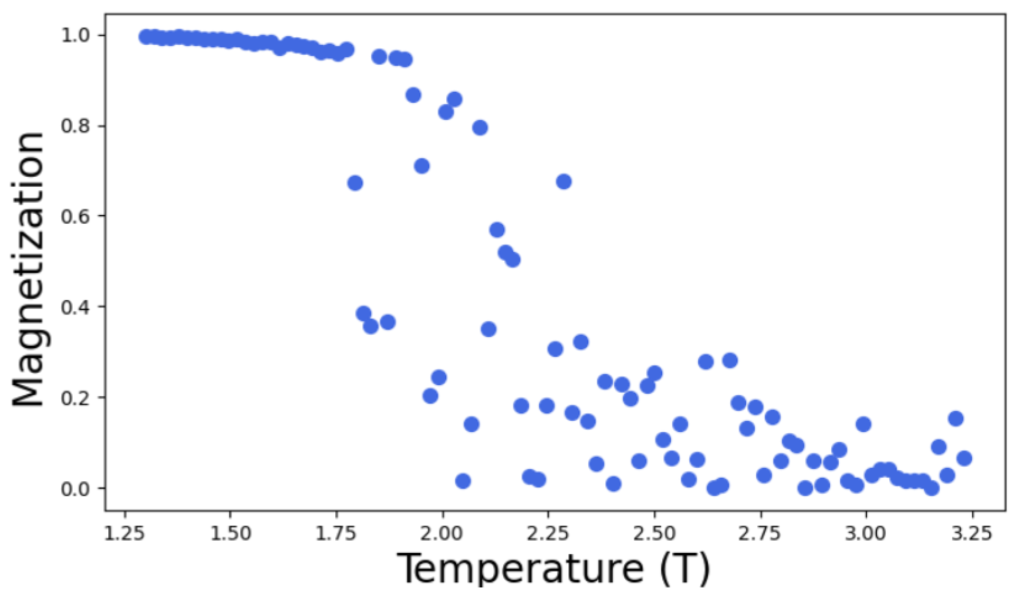
Figure 7.
Plot of Magnetization vs Temperature for lattice size L = 10
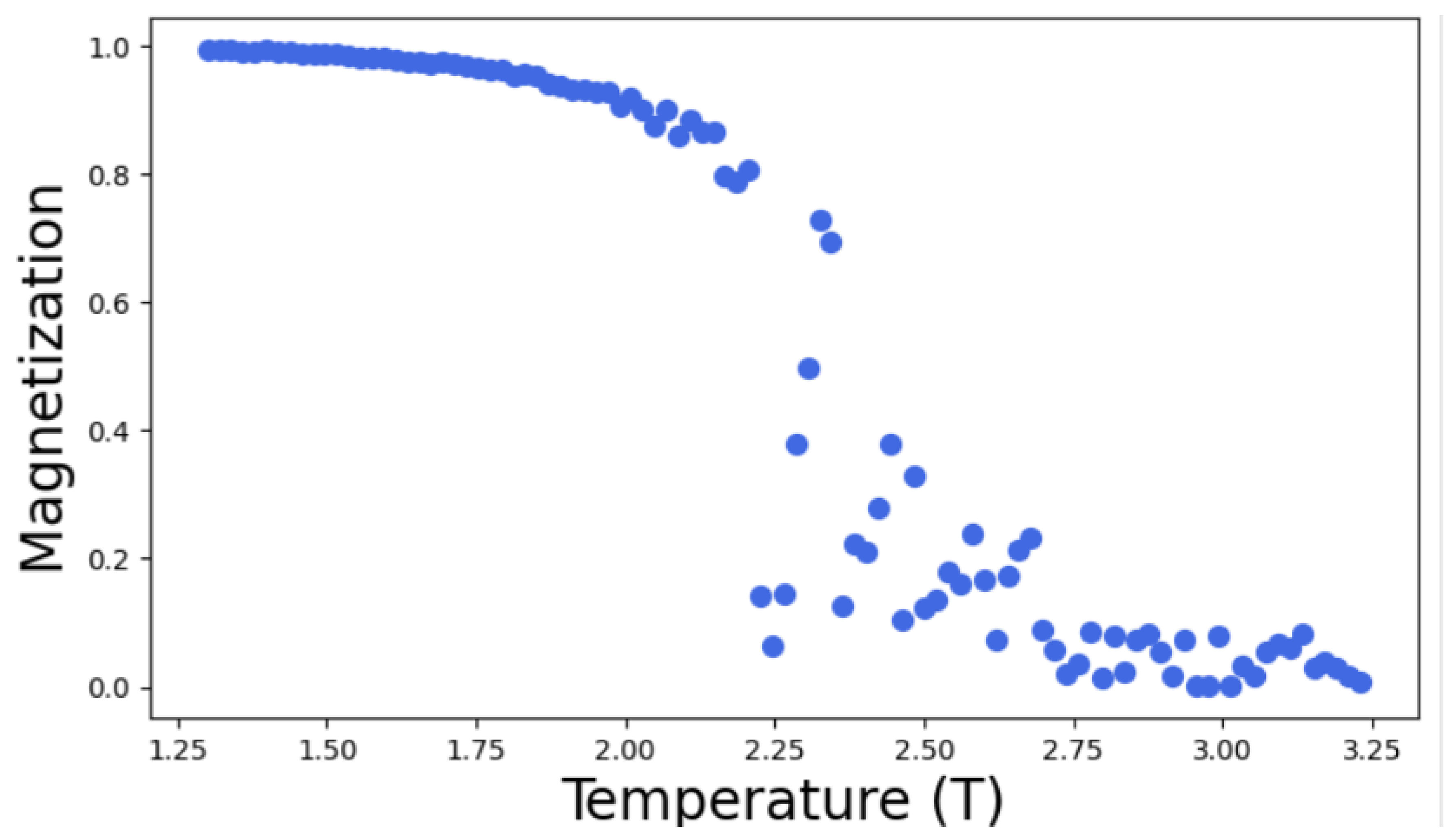
Figure 8.
Plot of Magnetization vs Temperature for lattice size L = 15
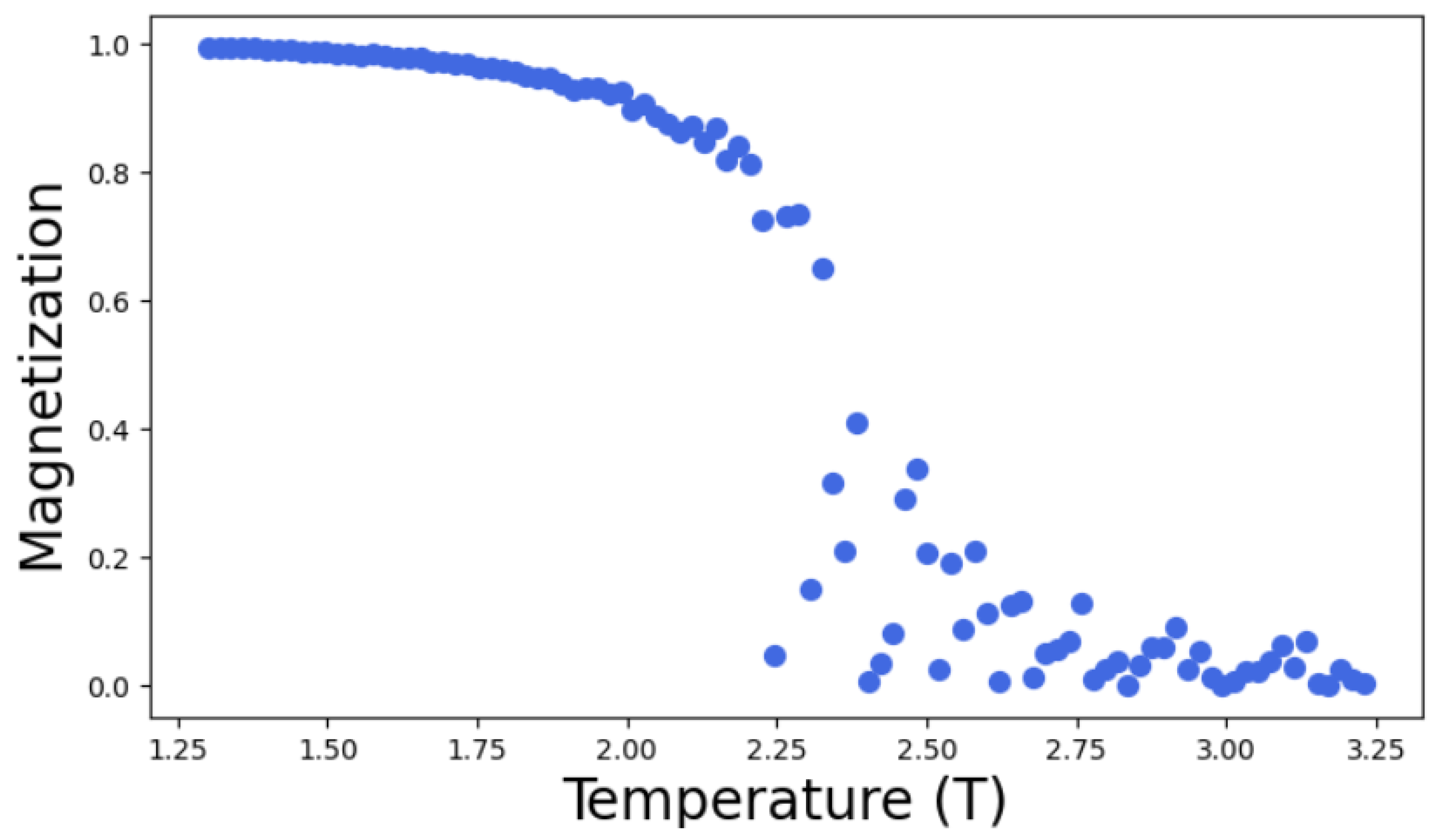
Figure 9.
Plot of Magnetization vs Temperature for lattice size L = 20
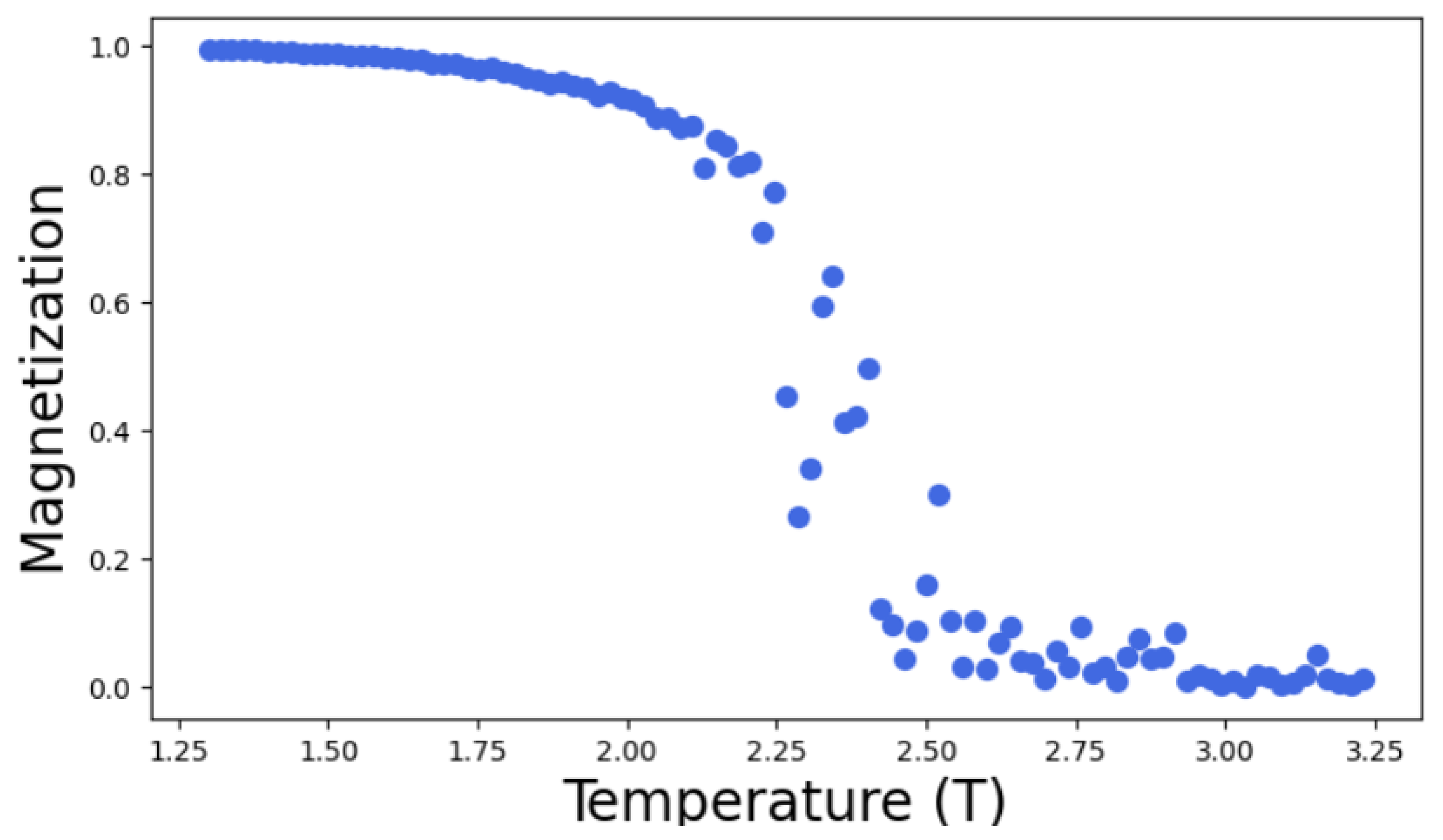
Figure 10.
Plot of Magnetization vs Temperature for lattice size L = 30
Disclaimer/Publisher’s Note: The statements, opinions and data contained in all publications are solely those of the individual author(s) and contributor(s) and not of MDPI and/or the editor(s). MDPI and/or the editor(s) disclaim responsibility for any injury to people or property resulting from any ideas, methods, instructions or products referred to in the content. |
© 2025 by the authors. Licensee MDPI, Basel, Switzerland. This article is an open access article distributed under the terms and conditions of the Creative Commons Attribution (CC BY) license (http://creativecommons.org/licenses/by/4.0/).
Copyright: This open access article is published under a Creative Commons CC BY 4.0 license, which permit the free download, distribution, and reuse, provided that the author and preprint are cited in any reuse.


