
Submitted:
20 August 2025
Posted:
22 August 2025
You are already at the latest version
Abstract
The extraction of ocean wave wavelengths from optical imagery via Fast Fourier Transform (FFT) exhibits significant potential for Wave-Derived Bathymetry (WDB). However, in practical applications, this method frequently produces anomalously large wavelength estimates. To date, there has been insufficient exploration into the mechanisms underlying image spectral leakage to low wavenumbers and its suppression strategies. This study investigates three plausible mechanisms contributing to spectral leakage in optical images and proposes a subimage-based preprocessing framework: prior to executing two-dimensional FFT, the remote sensing subimages employed for wavelength inversion undergo three sequential steps: (1) truncation of distorted pixel values using a Gaussian mixture model; (2) application of a polynomial detrending surface; (3) incorporation of a two-dimensional Hann window. Subsequently, the dominant wavenumber peak is localized in the power spectrum and converted to wavelength values. Water depth is then inverted using the linear dispersion equation, combined with wave periods derived from ERA5. Taking 2m-resolution WorldView-2 imagery of Sanya Bay, China as a case study, 1024m subimages are utilized, with validation conducted against chart-sounding data. Results demonstrate that the proportion of subimages with anomalous wavelengths is reduced from 18.9% to 3.3% (in contrast to 14.0%, 7.8%, and 16.6% when the three preprocessing steps are applied individually). Within the 0–20m depth range, the water depth retrieval accuracy achieves a Mean Absolute Error (MAE) of 1.79m; for the 20–40m range, the MAE is 6.38m. A sensitivity analysis of subimage sizes (512/1024/2048m) reveals that the 1024m subimage offers an optimal balance between accuracy and coverage. This method is both concise and effective, rendering it suitable for application in shallow-water WDB scenarios.
Keywords:
wave-derived bathymetry
; FFT
; anomalous wavelength
; outlier truncation
; detrending
; windowing
1. Introduction
Shallow-water bathymetry is a fundamental dataset for marine science and engineering. With the continuous expansion of human activities in areas such as marine resource exploitation, coastal engineering and protection, maritime safety, ecosystem management, and disaster early warning, the demand for high-resolution, rapidly updated nearshore bathymetric products has increased substantially [1,2,3,4]. Conventional shipborne sonar and airborne LiDAR bathymetry offer high accuracy, but their high cost, long acquisition cycles, and operational constraints limit large-area and time-critical surveys, particularly in shallow waters or along complex shorelines [5,6]. In contrast, satellite-derived bathymetry (SDB) provides extensive spatial coverage and repeat observation capabilities, enabling applications such as nautical chart updates, shoreline monitoring, and rapid post-disaster assessment at relatively low per-survey costs, and has become an important complementary approach for nearshore depth mapping [7,8].
The most widely applied SDB techniques are spectrally derived bathymetry methods, which utilize the systematic variation of light absorption and scattering in the water column, as well as bottom reflectance, with increasing depth in shallow waters. These methods map multispectral reflectance to depth through empirical or physics-based models, such as the depth invariant index method originally proposed by Lyzenga [9], the two-band log-ratio method by Stumpf [10], and the semi-analytical model by Lee [11,12]. However, these approaches rely heavily on high water transparency and on-site depth measurements for calibration [13,14,15]. Under favorable sea state and illumination conditions, alternating bright and dark bands caused by ocean surface waves appear in optical imagery, offering an alternative pathway for bathymetric retrieval—wave-derived bathymetry (WDB). This approach links the wavelength or phase speed extracted from imagery to water depth via the linear dispersion relation. WDB generally does not require in situ depth measurements for regression and is relatively insensitive to water turbidity, making it a promising technique for a broad range of applications [16,17,18].
Fast Fourier Transform (FFT) is a core technique for spectral analysis of remote sensing imagery to extract dominant ocean wave wavelengths and subsequently retrieve water depth, and has been successfully applied to both optical and SAR imagery [18,19,20,21]. However, in practical applications, this method frequently produces anomalous wavelength estimates [17,22,23,24]. Some researchers [16,25] attributed the anomalous wavelength retrievals to noise in remote sensing imagery and its more severe speckle. For subimage regions with abnormal wavelength retrievals, existing strategies include discarding the bathymetric results altogether [17,22], replacing FFT analysis with the spatial profile method (SPM) for either the entire study area or only the anomalous subimages [25,26]. In addition, various techniques have been proposed to mitigate the influence of such anomalies: Boccia [16] suggested resampling and filtering the imagery prior to spectral analysis, restricting the analysis domain, and applying spatial smoothing to parameters; Bian [27] introduced discrete convolution to smooth the wavelength field; and Mudiyanselage [24] applied a moving average to the retrieved wavelengths to reduce local deviations. These studies highlight the necessity of correcting FFT-based wavelength anomalies to improve both the spatial coverage and the accuracy of bathymetric retrieval.
The anomalies in wavelength inversion from remote sensing imagery using the FFT method arise because the analyzed energy spectrum peak shifts to other wavenumbers far from the expected value. Spectral analysis is a critical task in many military and civilian applications, such as performance testing of power and communication systems, mechanical vibration detection, and component linearity evaluation [28]. In these fields, researchers often encounter situations where the characteristic frequencies (or wavenumbers) of interest cannot be obtained from the energy spectra analyzed by the FFT method. Spectral leakage suppression is an important means of improving FFT-based spectral and wavelength analysis results. To address the various mechanisms that can generate spectral leakage, researchers have proposed a range of approaches, including filtering [29,30], detrending [31,32], windowing [28,33], and higher-order spectral analysis [34]. In current remote sensing wave wavelength analysis, improvements in spectral energy and wavelength estimation mainly rely on noise and speckle reduction, while other potential mechanisms and their corresponding solutions have not yet been thoroughly investigated.
This study systematically analyzes multiple mechanisms responsible for spectral leakage in FFT processing of remote sensing imagery and, for the first time, proposes an integrated image preprocessing approach to effectively suppress spectral leakage effects. The proposed method is validated through applications in ocean wave wavelength extraction and bathymetric retrieval. The remainder of this paper is organized as follows: Section 2 presents the principles of FFT-based wavelength extraction, the mechanisms of spectral anomalies and their correction, and the procedure for depth retrieval using the linear dispersion relation; Section 3 applies the methodology to a case study using WorldView-2 multispectral imagery; Section 4 discusses the influence of image subimage size on wavelength extraction and bathymetric retrieval accuracy; and Section 5 concludes the study.
2. Methods
2.1. FFT-Based Method for Wavelength Retrieval from Remote Sensing Imagery
A spatial (or temporal) data series can be regarded as the superposition of multiple wave components with different wavelengths (or periods). The Discrete Fourier Transform (DFT) is a commonly used method to identify the most dominant component among them. For remote sensing imagery containing ocean surface wave patterns, the DFT is first applied to compute the energy spectrum. The dominant wavenumber and corresponding wavelength, associated with the strongest spectral energy, are then determined from this spectrum [26,35].
Specifically, the remote sensing image is divided into multiple subimages of pixels, where the pixel resolution is ΔX, and the subimage side length is . Let the pixel value of the subimage be denoted as (). The two-dimensional DFT of the subimage is defined as
The corresponding wavenumber energy spectrum (power spectrum) is given by
where are the discrete indices, and the wavenumbers are given by and , where the wavenumber resolution is . In practice, the above DFT is efficiently computed using the Fast Fourier Transform (FFT); the computation is most efficient when is a power of two. After shifting the spectrum to center the zero frequency, the physical wavenumber range is equivalently represented as . From the location of the dominant spectral peak () in the wavenumber energy spectrum, the two-dimensional wavenumber vector of the dominant plane wave is obtained, and its dominant wavelength and wave direction are calculated as follows:
where .
In this study, an idealized regular wave field image is constructed in place of actual remote sensing imagery to illustrate the spectral characteristics obtained using the FFT method. Figure 1A shows the pixel value distribution of the regular wave field, generated from a sine function with a wavelength of 30 m. The crest lines (bright bands) are oriented at an angle of 30° to the y-axis, with a spatial resolution of 1 m per pixel and dimensions of 256×256 pixels. Figure 1B presents the energy spectrum derived from the image using the FFT method. The energy spectrum exhibits Hermitian symmetry, so only the Lower half needs to be analyzed. In Figure 1B, the maximum spectral energy occurs at , corresponding to a dominant wavelength of 29.8 m—slightly smaller than the constructed wavelength of 30 m. This discrepancy is primarily due to the finite FFT wavenumber resolution, non-integer wave cycles within the analysis window, and associated effects such as spectral leakage, direction quantization, and other discretization errors. Around the spectral peak, higher-energy sidelobes form clustered energy distributions, caused by finite-length, non-integer wavelength sampling of the regular wave. Additionally, a cross-shaped high-energy band passes through the spectral peak, resulting from discrete sampling along the inclined direction of the wave crests and troughs. Overall, when applying FFT to the regular wave field, spectral leakage produces clustered and cross-shaped high-energy patterns in the spectrum. However, because the leakage is not severe, the spectral energy near the actual wavelength remains dominant, and the identification of the dominant wavenumber and wavelength is not affected.
2.2. Correction Methods for Anomalous Wavelength Retrievals from Remote Sensing Imagery
2.2.1. Truncation of Distorted Pixel Values
in the spectral analysis of the FFT method, signal distortion is a common mechanism leading to spectral leakage [29,30]. For optical imagery with clearly defined ocean wave crests and troughs, factors such as breaking wave foam, wind-driven surface disturbances, underwater structures, oil slicks, and floating debris can introduce noise into the sea surface reflectance, often manifested as pronounced speckle. As a result, the pixel values contain small-scale distortion components. Therefore, this study incorporates the truncation of distorted pixel values as one of the approaches to suppress spectral leakage in optical imagery.
We apply a Gaussian Mixture Model (GMM) [36] to perform truncation of distorted pixel values. First, the frequency distribution of different pixel values in the optical image is computed. Then, a GMM is fitted to the pixel value–frequency distribution. The mathematical expression of the GMM is given by:
where denotes the pixel value, and is the frequency of occurrence of that pixel value. In Eq. (5), the first term on the right-hand side represents the primary component of the GMM, where is the amplitude, and and are the mean and standard deviation, respectively, describing the central tendency and dispersion of the pixel value distribution. The second term corresponds to the secondary component of the GMM, with , , and having analogous meanings to those of , , and . The parameters and are weighting coefficients, satisfying and . For optical imagery with clearly defined ocean wave crests and troughs, pixel values representing the wave pattern occur frequently, whereas distorted pixel values occur infrequently. Therefore, the parameters of the primary GMM component can be used to identify low-frequency distorted pixel values, which are then removed through truncation. The pixel value selection and truncation are expressed as:
Under the assumption of a normal distribution, the range of the primary component curve theoretically covers approximately 95.45% of the primary component pixels, with only about 4.55% classified as anomalies, while most distorted pixel values fall outside the range. After applying truncation based on this threshold, the FFT method is subsequently used to perform energy spectrum analysis on the corrected image.
In this study, a wave field image with artificially introduced noise was constructed to replace actual optical imagery in order to illustrate the mechanism by which truncation of distorted pixel values suppresses spectral leakage and improves anomalous wavelength retrievals. Figure 2A shows the pixel distribution containing noise, generated by superimposing 10 noise stripes produced by a random function onto the regular wave field of Figure 1A. The pixel values in Figure 1A range from –1 to 1, whereas in Figure 2A, the number of pixels exceeding 1 is 13,866 (maximum value 12.4), and the number of pixels less than –1 is 8,073 (minimum value –9.3). This yields a total of 21,939 anomalous pixels—approximately one-third of the image—indicating a substantial increase in distorted pixel values compared to the regular wave field.
The frequency distribution of pixel values in Figure 2A is shown in Figure 2B. Pixel values between –1 and 1 occur with high frequency, while those outside this range occur infrequently. Figure 2B also shows the Gaussian Mixture Model (GMM) fit to the pixel value frequency distribution, along with the fitted curves of its primary and secondary components. Within the –1 to 1 range, the GMM fit is dominated by the primary component, whereas outside this range, the secondary component dominates, effectively representing the contribution of distorted pixel values. For the primary component curve in Figure 2B, , are 0.0454 and 0.6592, respectively. Using these parameters in Eq. (6) to perform truncation of distorted pixel values yields cutoff thresholds of –1.2731 and 1.3638. The truncated pixel distribution is shown in Figure 2C, where the particularly bright and dark noise spots have been removed.
Energy spectrum analysis was performed on the pixel values of Figures 2A and 2C using FFT, with results shown in Figures 2D and 2E, respectively. In Figure 2D, the high-energy spectrum is concentrated in a clustered region, interspersed with several high-energy streaks. The maximum energy occurs at , corresponding to a dominant wavelength of 256 m. Compared with Figure 1B, the presence of distorted pixel values causes severe leakage of energy toward low wavenumbers in the far field, significantly altering both the shape of the spectrum and the location of its maximum, resulting in a dominant wavelength estimate that deviates substantially from the actual value. In contrast, the high-energy spectral distribution in Figure 2E is more dispersed, with the maximum occurring at , corresponding to a dominant wavelength of 29.8 m. These results indicate that a large number of distorted pixel values leads to severe energy leakage toward low wavenumbers in the FFT spectrum; applying truncation of distorted pixel values can mitigate the resulting anomalous wavelengths caused by spectral leakage and correct the retrieved wavelength.
2.2.2. Detrending of Non-Stationary Pixel Values
In spectral analysis research, it has been observed that non-stationary variations in a signal can cause spectral leakage, and removing the trend surface associated with such variations can effectively suppress this phenomenon [31,32]. In optical imagery, pixel values are influenced by bottom-reflected spectra, which are themselves affected by seabed slope and spatial variations in water turbidity. These factors can superimpose large-scale non-stationary trend surfaces onto the sea surface reflectance spectra. In addition, uneven illumination may also induce large-scale non-stationary variations in sea surface reflectance. Therefore, this study incorporates detrending of non-stationary pixel values as one of the approaches to suppress spectral leakage in optical imagery.
The detrending method proposed by Vieira [37,38] is employed in this study, using a two-dimensional quadratic polynomial to fit the non-stationary trend surface:
where is the estimated trend surface, X and Y are the coordinate positions and , , , , and are the regression parameters estimated by the least squares method. This surface is then subtracted from the originals generating a new variable which we are calling residuals.
The residuals obtained after detrending are subsequently used in the FFT-based energy spectrum analysis.
In this study, a wave field image containing a trend surface was constructed in place of actual remote sensing imagery to illustrate the mechanism by which detrending suppresses spectral leakage and improves anomalous wavelength retrievals. Figure 3A shows the pixel value distribution containing the trend surface, generated by superimposing the non-stationary trend surface defined in Eq. (7) onto the regular wave field of Figure 1A. While Figure 3A still exhibits pronounced wave features, the pixel values in the lower portion of the image are noticeably higher than those in the upper portion due to the influence of the trend surface.
Figure 3B presents the energy spectrum of Figure 3A computed using the FFT method. It is generally similar to that of Figure 1B, but with an additional high-energy region at low wavenumbers; the maximum energy occurs at , corresponding to a wavelength of 256 m. A two-dimensional quadratic polynomial was fitted to the pixel values of Figure 3A, and the resulting trend surface is shown in Figure 3C, which increases from the upper part of the domain toward the lower part. The energy spectrum of Figure 3C, obtained via FFT, is shown in Figure 3D and reveals a distinct high-energy band at low wavenumbers. The maximum energy is again located at , with a magnitude nearly identical to that in Figure 3B, corresponding to a wavelength of 256 m.
These results demonstrate that the parabolic variation of the trend surface across the entire domain manifests in the FFT spectrum as concentrated energy at low wavenumbers, which is the root cause of the anomalous wavelength retrieval observed in Figure 3A. Detrending effectively suppresses the energy leakage to remote low wavenumbers, thereby correcting the retrieved wavelength.
2.2.3. Windowing to Suppress Edge Discontinuities
The FFT method segments the signal data into multiple subimages and performs energy spectrum analysis on each subimage. Discontinuous changes in data values at the subimage edges can cause spectral leakage, and windowing is a common technique used to suppress such leakage [28,33]. When applying FFT-based spectral analysis to optical imagery, discontinuities in pixel values at subimage edges can also occur. Due to the significant difference in spectral reflectance between seawater and land, some subimages may contain both ocean and land areas, further exacerbating the discontinuity problem at the edges.
In this study, a two-dimensional Hann window is applied to each subimage to suppress spectral leakage caused by discontinuous pixel values along subimage edges. The expression of the two-dimensional Hann window function is given as [39]:
Here, M and N are the pixel dimensions of the subimage, and m and n are the pixel indices, where , . It can be seen that has a value of 1 at the center of the subimage and decreases to 0 toward the edges. The Hann window is applied by multiplying the subimage pixel values by the window function to produce new pixel values, which are then analyzed using the FFT method to compute the spectral energy. This procedure effectively suppresses spectral leakage caused by discontinuities in edge data.
A wave field image with edge discontinuities was constructed in place of actual remote sensing imagery to illustrate the mechanism by which windowing suppresses spectral leakage and improves anomalous wavelength retrievals. Starting from the regular wave image in Figure 1A, a 20 m-wide strip near the left boundary was assigned a constant pixel value of –1, resulting in a wave field image with an edge discontinuity (Figure 4A). The energy spectrum of the pixel values in Figure 4A, shown in Figure 4B, retains the spectral characteristics of the regular wave field in Figure 1B but exhibits additional elongated high-energy bands, with the maximum spectral energy occurring at , , corresponding to a wavelength of 256 m.
Figure 4C shows the pixel value distribution after applying the Hann window, where the pixel values at the image edges approach zero while the central region retains the wave features. The energy spectrum of Figure 4C, presented in Figure 4D, shows that the elongated high-energy bands are suppressed and clustered high-energy regions dominate. The maximum spectral energy now occurs at , corresponding to a dominant wavelength of 29.8 m. These results indicate that discontinuities in edge pixel values cause energy leakage toward remote low wavenumbers, leading to anomalous wavelength retrievals. Applying windowing effectively suppresses this spectral leakage and corrects the retrieved wavelength.
2.3. Depth Inversion from Remotely Sensed Wavelengths
Based on wavelength information retrieved from remote sensing imagery, shallow-water bathymetry can be derived using the linear wave dispersion relation. The linear dispersion relation is given as [40]:
where ω denotes the angular wave frequency, denotes the wave period, . g is the gravitational acceleration, is the wavenumber, is the wavelength,. denotes the deep-water wavelength. is the water depth.
Under deep-water conditions(), , the dispersion relation can be approximated as:
In deep water, the wavelength is almost independent of water depth, and thus depth inversion from wavelength is not feasible. In contrast, under shallow-water conditions(), water depth becomes a significant factor influencing wavelength, making wavelength-based depth inversion possible. In this case, the bathymetry can be derived from the following equation obtained from Eq. (10):
where is provided by the remotely sensed wavelength retrieval, and can be estimated by substituting the deep-water wavelength into Eq(11) [19,22,35], or obtained from other sources.
3. Case Study: Wavelength Retrieval and Bathymetry Inversion in Sanya Bay
3.1. Study Area and Data
The study area is located in Sanya Bay, situated on the southern coast of Hainan Island, China. The remote sensing dataset used in this study is a WorldView-2 image acquired on 5 August 2019 at 03:30 UTC. WorldView-2, launched by DigitalGlobe (USA) in 2009, is a high-resolution commercial Earth observation satellite with outstanding spatial and spectral imaging capabilities. It carries one panchromatic band (spatial resolution of 0.5 m) and multiple multispectral bands (spatial resolution of 2.0 m) covering wavelengths from the visible to the near-infrared region. The sensor has been widely used in applications such as urban mapping, coastal monitoring, agricultural surveys, and environmental assessment, and is an important data source for high-resolution remote sensing analysis. The WorldView-2 image of the study area is shown in Figure 5A, where clear alternating bright-and-dark ripple patterns are visible. For wavelength analysis and bathymetric inversion, we selected the red band from the multispectral dataset, which is sensitive to ocean surface roughness [41], with a spatial resolution of 2.0 m.
For the validation of wave-derived bathymetry results, we used nautical chart data based on in situ depth measurements (Figure 5B), which were provided by the China Communications Press in 2020. A total of 350 charted points are available within the study area. The water depths in Figure 5B do not exceed 40 m, indicating that the maximum depth in this region may not satisfy the deep-water wave criterion. For instance, when the wave crest period is 8 s, Eq. (11) combined with the deep-water criterion yields a required depth of 49.9 m. Therefore, instead of deriving the wave period from remotely sensed wavelengths, we adopted wave period data from the ERA5 numerical reanalysis wave product provided by the European Centre for Medium-Range Weather Forecasts (ECMWF). The ERA5 dataset has a temporal resolution of 1 hour and a spatial resolution of 0.5o. The reliability of ERA5 wave period data for Sanya Bay has been assessed and validated in Liu[26]. For the acquisition time corresponding to the WorldView-2 image, the ERA5 wave product reported a mean wave period of 6 s. Based on the statistical relationship between peak wave period and mean wave period [42,43], the peak wave period was determined to be 8.46 s.
3.2. Wavelength Retrieval Results Without Spectral Leakage Suppression
The WorldView-2 image was divided into multiple subimages, and the FFT method was applied to each subimage to compute the power spectrum. The dominant wavelength was identified from the spectral peak and assigned to the center of each subimage. Each subimage consisted of 512×512 pixels, corresponding to a spatial extent of 1024m. The spacing between adjacent subimage centers was set to 60 m, resulting in partial overlap among neighboring subimages. For the WorldView-2 acquisition, the corresponding wave period was 8.46 s. Using Eq. (11), the deep-water wavelength associated with this period was calculated as 111.8 m. Any retrieved wavelength larger than this value was considered an anomalous wavelength that cannot be used for depth inversion.
Figure 6A presents the wavelength retrieval results without spectral leakage suppression. Numerous anomalies can be observed: among a total of 16,738 subimages, 3,103 exhibited anomalous wavelength values, accounting for 18.9% of the total. The anomalous wavelengths ranged from 111.8 m to 1024m, with the majority equal to 1024m. These anomalies were distributed not only near the shoreline and along the image boundaries but also within the central portion of the image.
3.3. Wavelength Retrieval Results with Spectral Leakage Suppression
3.3.1. Results After Truncation of Distorted Pixel Values
For subimages with anomalous wavelength values, three preprocessing approaches—truncation of distorted pixel values, detrending, and windowing—were first applied individually, followed by their combined application, to analyze the wavelength retrieval results.
Figure 6B presents the wavelength retrieval results after truncation of distorted pixel values from the WorldView-2 image. The number of subimages with anomalous wavelengths was reduced to 2,288, accounting for 14.0% of the total subimages. Compared with the unsuppressed results (Figure 6A), spectral leakage was effectively suppressed in 815 subimages, and their wavelength retrievals were corrected. Most of these corrected subimages were located in the lower-left portion of the image. One representative subimage from this region (outlined by rectangle 1 in Figure 5A) was selected to illustrate the suppression of spectral leakage through pixel-value truncation.
The original subimage is shown in Figure 7A, where the lower-right corner exhibits stronger brightness contrasts. The corresponding energy spectrum derived from the original subimage is presented in Figure 7B: the maximum spectral energy occurred in the central low-wavenumber region, at , corresponding to a wavelength of 1024m. After truncation of distorted pixel values, the spatial distribution of pixel intensities (Figure 7C) became more homogeneous across the subimage. The corresponding energy spectrum (Figure 7D) indicates that the maximum spectral energy shifted toward higher wavenumbers, located at , corresponding to a wavelength of 100.4 m.
Overall, distorted pixel values in this subimage caused part of the spectral energy to leak toward remote low wavenumbers, resulting in anomalous wavelength retrievals. The truncation of distorted pixel values effectively suppressed spectral leakage, corrected the anomalous wavelength, and verified the effectiveness of the method described in Section 2.2.1.
3.3.2. Results After Detrending of Pixel Values
Figure 6C shows the wavelength retrieval results after detrending the pixel values of the WorldView-2 image. The number of subimages with anomalous wavelengths was reduced to 1,278, accounting for 7.8% of the total. Compared with the unsuppressed results (Figure 6A), spectral leakage was suppressed in 1,825 subimages, and their wavelength retrievals were corrected. A representative subimage from this group (outlined by rectangle 2 in Figure 5A) was selected to illustrate the suppression effect of detrending.
The original subimage is presented in Figure 8A, and its energy spectrum (Figure 8B) shows that the maximum spectral energy occurred in the central low-wavenumber region at , , corresponding to a wavelength of 1024m. The fitted trend surface derived from Figure 8A is shown in Figure 8E. After detrending, the pixel distribution (Figure 8C) became more uniform, and the slow increase in pixel values from the upper left to the lower right corner was effectively suppressed. The corresponding energy spectrum of the detrended subimage (Figure 8D) indicates that the maximum energy shifted toward higher wavenumbers, located at , corresponding to a wavelength of 73.1 m. These results demonstrate that detrending effectively suppressed spectral leakage and corrected the anomalous wavelength estimate.
The original subimage is presented in Figure 8A, and its energy spectrum (Figure 8B) shows that the maximum spectral energy occurred in the central low-wavenumber region at , , corresponding to a wavelength of 1024m. The fitted trend surface is shown in Figure 8E, indicating a subtle increasing trend from the upper left to the lower right of the original subimage that is not easily discernible directly. The residual image after detrending is displayed in Figure 8C. Its corresponding energy spectrum (Figure 8D) indicates that the maximum energy shifted toward higher wavenumbers, located at , corresponding to a wavelength of 73.1 m. These results demonstrate that detrending effectively suppressed spectral leakage, corrected the anomalous wavelength, and verified the effectiveness of the method described in Section 2.2.2.
3.3.3. Results After Windowing of Subimages
Figure 6D shows the wavelength retrieval results from the WorldView-2 image after applying the windowing technique. The number of subimages with anomalous wavelengths was reduced to 2,719, accounting for 16.6% of the total. Compared with the unsuppressed results (Figure 6A), spectral leakage was suppressed and wavelength anomalies were corrected in 384 subimages. These corrected subimages were mainly distributed near the coastline.
A representative subimage from this group (outlined by rectangle 3 in Figure 5A) was selected for detailed analysis of the spectral leakage suppression effect. The original subimage is presented in Figure 9A, where a land–water boundary is evident near the upper edge, with significant radiometric differences between land and water pixels. The corresponding energy spectrum (Figure 9B) shows maximum energy located near the central low-wavenumber region at , , corresponding to a wavelength of 1024m.
After applying the Hann window, the pixel distribution is shown in Figure 9C. The boundary pixels were effectively down-weighted, while the central region retained clear wave patterns. The energy spectrum of the windowed subimage (Figure 9D) indicates that the maximum energy shifted toward higher wavenumbers, at , corresponding to a wavelength of 64 m. These results demonstrate that the windowing technique effectively suppressed spectral leakage, corrected the anomalous wavelength, and verified the effectiveness of the method described in Section 2.2.3.
3.3.4. Wavelength Retrieval Results After Combined Spectral Leakage Suppression
The preceding subsections demonstrated that truncation of distorted pixel values, detrending of pixel values, and windowing—when applied individually—were each able to suppress spectral leakage in some subimages and correct anomalous wavelength estimates. This indicates that spectral leakage in the remote sensing imagery is caused by multiple mechanisms and therefore requires a combined approach for effective suppression.
Figure 6E presents the wavelength retrieval results after applying the combined suppression method. The number of subimages with anomalous wavelengths was reduced to only 536, accounting for 3.3% of the total. This demonstrates that spectral leakage toward remote low wavenumbers, which caused most of the anomalous wavelengths, was effectively suppressed. The remaining anomalous subimages were primarily located near the coastline, where a large proportion of land pixels limited the effectiveness of the windowing technique. Overall, as shown in Figure 6E, the corrected wavelengths exhibit a clear trend of increasing from the coast toward the open sea, which is consistent with the spatial distribution of water depth.
3.4. Bathymetric Results from Wave-Derived Wavelengths
Using the wavelength retrieval results obtained from the combined spectral leakage suppression method (Figure 6E), water depths were calculated based on Equation (12) and further corrected for tidal effects. The inversion results are shown in Figure 10A, where depths increase from the coast toward the open sea, consistent with the trend observed in the nautical chart depths (Figure 5B). For error analysis, the charted points in Figure 5B were taken as centers, and all subimage-derived depths within a 30 m radius were matched to the nearest neighbor. Out of the 350 charted points, 337 had valid matches. As shown in Figure 10B, the overall mean error (ME) of these points was –1.57 m, with a mean absolute error (MAE) of 3.31 m and a correlation coefficient (R) of 0.80. For depths of 0–20m, the MAE was 1.79 m, while for depths of 20–40m, the MAE increased to 6.38 m. These results indicate that depth inversion performs better in shallow waters, whereas the error increases with depth. The underlying reason is that the rate of change of wavelength with respect to depth (dL/dh) decreases as depth increases, amplifying inversion errors.
We also selected subimages where anomalous wavelength values had been corrected, yielding matches with 47 charted points for error analysis (Figure 10C). For this subset, the overall Mean Error (ME) was –2.49 m, the MAE was 3.37 m, and R was 0.86. In the 0–20m depth range, the MAE was 1.44 m, while in the 20–40m range it increased to 6.97 m. The bathymetric errors from these corrected subimages were comparable to those from all subimages, demonstrating that spectral leakage suppression and the correction of anomalous wavelength values are meaningful for improving wave-derived bathymetry.
4. Discussion
In the spectral energy analysis using the FFT method, the choice of subimage size has a significant impact on the results [44,45]. However, for wavelength retrieval from optical remote sensing imagery, there has been little in-depth investigation into how different spectral leakage mechanisms are affected by subimage size. In Section 3, the subimage size of the WorldView-2 imagery was set to 1024m. Here, we further set the subimage sizes to 512m and 2048m, while keeping the distance between subimage centers at 60 m, to perform additional wavelength retrieval experiments.
Figure 11A–E presents the wavelength retrieval results with a subimage size of 512m. Figure 11A shows the retrieval without spectral leakage suppression, where the total number of subimages is 16,378, among which 1,313 subimages exhibit anomalous wavelengths, accounting for 8%. Compared with Figure 6A (subimage size of 1024m), the proportion of anomalous subimages is significantly reduced. As shown in Figures 11B–D, after applying distortion truncation, detrending, and windowing techniques, the proportions of anomalous subimages decrease to 6%, 3.1%, and 3.8%, respectively, indicating that spectral leakage is still dominated by low-wavenumber leakage caused by trend surfaces. Compared with Figures 6B–D, reducing the subimage size results in a smaller impact area for all three spectral leakage mechanisms, with the effect of windowing showing greater variability. Figure 11E shows the wavelength retrieval results obtained by combining all three suppression methods. The number of anomalous subimages is reduced to 222, accounting for 1.4% of the total. Compared with Figure 6F, the spatial extent of anomalous wavelengths near the coastline is reduced, while little change is observed elsewhere.
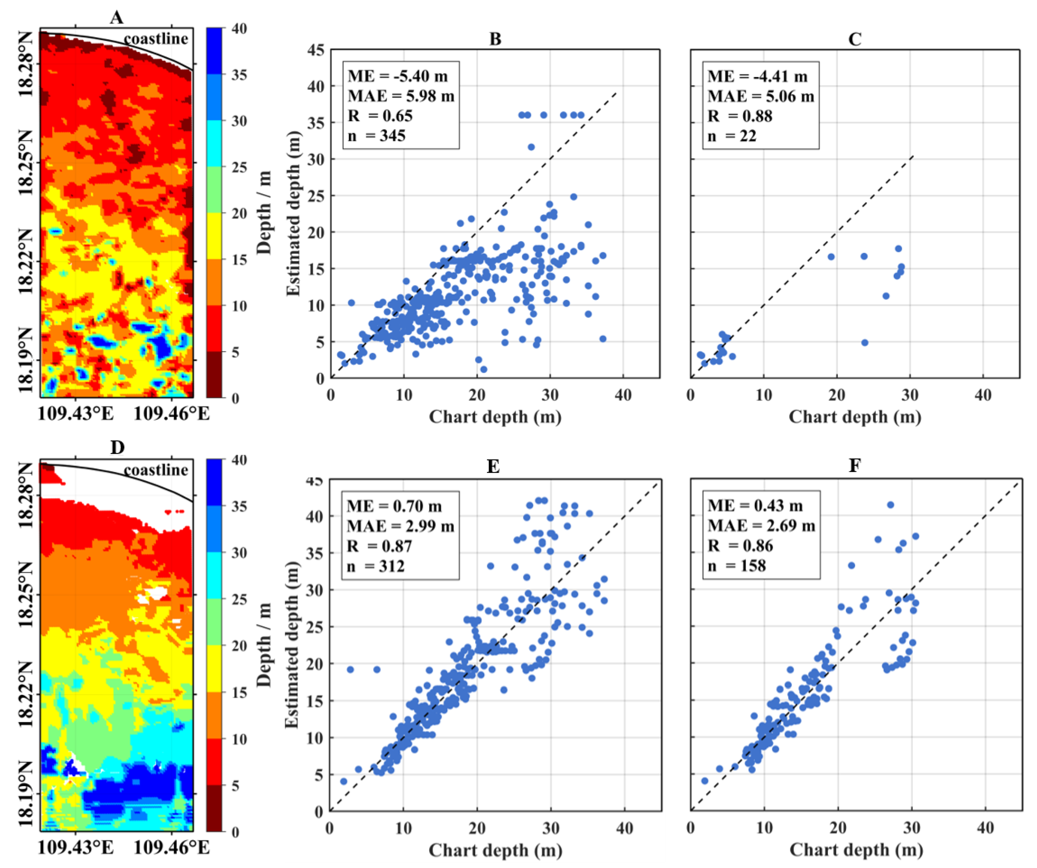
Figure 12A–C presents the wave-derived bathymetry results and error analysis for subimages of 512m. Using the charted points shown in Figure 5B as centers, all subimage-derived depths within a 30 m radius were matched to the nearest chart depth. Among the 350 charted points, 345 were successfully matched. For these points, the overall mean error (ME) was –5.4 m, the mean absolute error (MAE) was 5.98 m, and the correlation coefficient (R) was 0.65. The MAE was 3.05 m for depths of 0–20m and increased to 12.04 m for depths of 20–40m. For subimages with corrected anomalous wavelengths, 22 charted points were matched, yielding an overall ME of –4.4 m, an MAE of 5.06 m, and an R value of 0.88. The MAE was 1.62 m for depths of 0–20m and 14.02 m for depths of 20–40m. Compared with the results obtained using 1024m subimages (Figure 10A–C), the inversion errors increased overall, but the performance in nearshore regions was markedly better.
Figure 11F–J presents the wavelength retrieval results with a subimage size of 2048m. Figure 11F shows the retrieval without spectral leakage suppression, where the total number of subimages is 16,378, among which 9,891 subimages exhibit anomalous wavelengths, accounting for 60.4%. Compared with Figure 6A (subimage size of 1024m), the proportion of anomalous subimages increases substantially. As shown in Figures 11G–I, after applying distortion truncation, detrending, and windowing techniques, the proportions of anomalous subimages are reduced to 48.0%, 17.5%, and 58.8%, respectively, indicating that spectral leakage remains dominated by low-wavenumber leakage caused by trend surfaces. Compared with Figures 6B–D, enlarging the subimage size considerably expands the affected areas for all three spectral leakage mechanisms, with the trend surface effect showing the greatest increase.Figure 11J shows the retrieval results obtained by combining all three suppression methods. The number of anomalous subimages is reduced to 2,029, accounting for 12.4% of the total. Compared with Figure 6F, the extent of anomalous wavelengths expands near the coastline, and some anomalies remain uncorrected elsewhere.
Figure 12D–F presents the wave-derived bathymetry results and error analysis for subimages of 2048m. Using the charted points shown in Figure 5B as centers, all subimage-derived depths within a 30 m radius were matched to the nearest chart depth. Among the 350 charted points, 312 were successfully matched. For these points, the overall mean error (ME) was –0.7 m, the mean absolute error (MAE) was 2.99 m, and the correlation coefficient (R) was 0.87. The MAE was 1.69 m for depths of 0–20m and 5.26 m for depths of 20–40m. For subimages with corrected anomalous wavelengths, 158 charted points were matched, yielding an overall ME of 0.43 m, an MAE of 2.69 m, and an R value of 0.86. The MAE was 1.45 m for depths of 0–20m and 7.29 m for depths of 20–40m. Compared with the results obtained using 1024m subimages (Figure 10A–C), the inversion errors decreased, with a notably improved accuracy in deeper-water regions.
5. Conclusions
In wave-derived bathymetry (WDB) research, the FFT method sometimes produces energy spectrum peaks concentrated at low wavenumbers, leading to abnormally large wavelength retrievals that interfere with depth inversion. Existing studies have mainly attempted to correct these anomalies by suppressing noise and speckle effects. Focusing on optical remote sensing imagery, this study identifies three mechanisms that may cause spectral peaks to cluster at low wavenumbers: (1) distorted pixel values induced by surface reflection noise and speckle; (2) non-stationary variations of pixel values driven by seabed reflectance and wave height changes; and (3) discontinuities in subimage edge pixels caused by land–sea boundaries. Based on these mechanisms, we designed a hybrid correction method for abnormal wavelength retrievals, consisting of truncating distorted pixel values with a Gaussian Mixture Model (GMM), fitting and removing a quadratic polynomial trend surface to eliminate non-stationary variations, and applying a window function to suppress edge discontinuities.
In this study, a WorldView-2 image of Sanya Bay was analyzed using the FFT method to derive WDB from the dominant wavelengths identified in the energy spectrum. When the subimage size was set to 1024m, anomalous wavelength subimages accounted for 18.9% of the total. By applying distortion truncation, detrending, and windowing techniques to suppress energy leakage toward remote low wavenumbers, the proportion of anomalous subimages was reduced to 14.0%, 7.8%, and 16.6%, respectively. These results indicate that non-stationary pixel trends are the primary cause of wavelength anomalies, while the other two mechanisms also contribute. When the three methods were combined, anomalous subimages decreased to only 3.3%, and most anomalous wavelength values were corrected. Using the corrected wavelengths for depth inversion, the mean absolute error (MAE) was 1.79 m in the 0–20m shallow-water zone and 6.38 m in the 20–40m zone, confirming good applicability in shallow waters. We also performed wavelength inversion and depth estimation with subimage sizes of 512m and 2048m. Results showed that reducing subimage size decreased the extent of anomalous regions but increased overall depth errors due to other wavelength inaccuracies, while enlarging subimage size increased anomalous regions but reduced overall depth errors. In practical applications, subimage size should therefore be selected by balancing multiple factors.
This study addresses the issue of anomalously large wavelength values in optical imagery inversion by proposing methods to suppress the migration of spectral energy toward remote low wavenumbers, thereby correcting wavelength anomalies. However, noise, speckle, and other factors in optical imagery may also cause energy to migrate toward other local wavenumbers or higher wavenumbers, leading to different forms of wavelength inversion errors that degrade bathymetric accuracy. The methods proposed in this study are not yet sufficient to fully resolve these issues. Future research will further investigate these problems and develop corresponding solutions.
Conflicts of Interest
The authors declare no conflicts of interest.
References
- Almar, R. Pan-European Satellite-Derived Coastal Bathymetry—Review, User Needs and Future Services. Frontiers in Marine Science 2021, 8. [Google Scholar] [CrossRef]
- Huang, R.; Yu, K.; Wang, Y.; Wang, J.; Mu, L.; Wang, W. Bathymetry of the Coral Reefs of Weizhou Island Based on Multispectral Satellite Images. Earth-Science Reviews. [CrossRef]
- Mavraeidopoulos, A.K.; Pallikaris, A.; Oikonomou, E. Satellite Derived Bathymetry (SDB) and Safety of Navigation. International Hydrographic Review 2017. [Google Scholar]
- Pe’eri, S.; Parrish, C.; Azuike, C.; Alexander, L.; Armstrong, A. Satellite Remote Sensing as a Reconnaissance Tool for Assessing Nautical Chart Adequacy and Complete. Marine Geodesy 2014. [Google Scholar] [CrossRef]
- Grządziel, A. Method of Time Estimation for the Bathymetric Surveys Conducted with a Multi-Beam Echosounder System. Applied Sciences 2023, 13, 10139. [Google Scholar] [CrossRef]
- Saylam, K.; Hupp, J.R.; Andrews, J.R.; Averett, A.R.; Knudby, A.J. Quantifying Airborne Lidar Bathymetry Quality-Control Measures: A Case Study in Frio River, Texas. Sensors 2018, 18, 4153. [Google Scholar] [CrossRef]
- Ferreira, I.O.; Andrade, L.C.D.; Teixeira, V.G.; Santos, F.C.M. State of Art of Bathymetric Surveys. Bol. Ciênc. Geod. 2022, 28, e2022002. [Google Scholar] [CrossRef]
- He, J.; Zhang, S.; Cui, X.; Feng, W. Remote Sensing for Shallow Bathymetry: A Systematic Review. 2024.
- Lyzenga, D.R. Passive Remote Sensing Techniques for Mapping Water Depth and Bottom Features. Appl. Opt. 1978, 17, 379. [Google Scholar] [CrossRef] [PubMed]
- Stumpf, R.P.; Holderied, K.; Sinclair, M. Determination of Water Depth with High-resolution Satellite Imagery over Variable Bottom Types. Limnology & Oceanography 2003, 48, 547–556. [Google Scholar] [CrossRef]
- Lee, Z.; Carder, K.L.; Mobley, C.D.; Steward, R.G.; Patch, J.S. Hyperspectral Remote Sensing for Shallow Waters. I. A Semianalytical Model. Optical Society of America 1998. [Google Scholar] [CrossRef]
- Lee, Z.; Carder, K.L.; Mobley, C.D.; Steward, R.G.; Patch, J.S. Hyperspectral Remote Sensing for Shallow Waters: 2. Deriving Bottom Depths and Water Properties by Optimization. Optical Society of America 1999. [Google Scholar] [CrossRef]
- Casal, G. Assessment of Empirical Algorithms for Bathymetry Extraction Using Sentinel-2 Data. International Journal of Remote Sensing 2018. [Google Scholar] [CrossRef]
- Kutser, T.; Vahtmäe, E.; Praks, J. A Sun Glint Correction Method for Hyperspectral Imagery Containing Areas with Non-Negligible Water Leaving NIR Signal. 2009.
- Brusch, S.; Held, P.; Lehner, S.; Rosenthal, W.; Pleskachevsky, A. Underwater Bottom Topography in Coastal Areas from TerraSAR-X Data. International Journal of Remote Sensing 2011, 32, 4527–4543. [Google Scholar] [CrossRef]
- Boccia, V.; Renga, A.; Moccia, A.; Zoffoli, S. Tracking of Coastal Swell Fields in SAR Images for Sea Depth Retrieval: Application to ALOS L-Band Data. IEEE J. Sel. Top. Appl. Earth Observations Remote Sensing 2015, 8, 3532–3540. [Google Scholar] [CrossRef]
- Danilo, C.; Melgani, F. Wave Period and Coastal Bathymetry Using Wave Propagation on Optical Images. IEEE Trans. Geosci. Remote Sensing 2016, 54, 6307–6319. [Google Scholar] [CrossRef]
- Brusch, S.; Held, P.; Lehner, S.; Rosenthal, W.; Pleskachevsky, A. Underwater Bottom Topography in Coastal Areas from TerraSAR-X Data. International Journal of Remote Sensing 2011, 32, 4527–4543. [Google Scholar] [CrossRef]
- Bergsma, E.W.J.; Almar, R.; Maisongrande, P. Radon-Augmented Sentinel-2 Satellite Imagery to Derive Wave-Patterns and Regional Bathymetry. Remote Sensing 2019, 11, 1918. [Google Scholar] [CrossRef]
- Pereira, P.; Baptista, P.; Cunha, T.; Silva, P.A.; Romão, S.; Lafon, V. Estimation of the Nearshore Bathymetry from High Temporal Resolution Sentinel-1A C-Band SAR Data - A Case Study. Remote Sensing of Environment 2019, 223, 166–178. [Google Scholar] [CrossRef]
- Poupardin, A.; Idier, D.; De Michele, M.; Raucoules, D. Water Depth Inversion From a Single SPOT-5 Dataset. IEEE Trans. Geosci. Remote Sensing 2016, 54, 2329–2342. [Google Scholar] [CrossRef]
- Huang, L.; Meng, J.; Fan, C.; Zhang, J.; Yang, J. Shallow Sea Topography Detection from Multi-Source SAR Satellites: A Case Study of Dazhou Island in China. Remote Sensing 2022, 14, 5184. [Google Scholar] [CrossRef]
- Leu, L.-G.; Chang, H.-W. Remotely Sensing in Detecting the Water Depths and Bed Load of Shallow Waters and Their Changes. Ocean Engineering 2005, 32, 1174–1198. [Google Scholar] [CrossRef]
- Mudiyanselage, S.D.; Wilkinson, B.; Abd-Elrahman, A. Automated High-Resolution Bathymetry from Sentinel-1 SAR Images in Deeper Nearshore Coastal Waters in Eastern Florida. Remote Sensing 2023, 16, 1. [Google Scholar] [CrossRef]
- Li, J.; Zhang, H.; Hou, P.; Fu, B.; Zheng, G. Mapping the Bathymetry of Shallow Coastal Water Using Single-Frame Fine-Resolution Optical Remote Sensing Imagery. Acta Oceanol. Sin. 2016, 35, 60–66. [Google Scholar] [CrossRef]
- Liu, M.; Zhu, S.; Cheng, S.; Zhang, W.; Cao, G. Nearshore Depth Estimation Using Fine-Resolution Remote Sensing of Ocean Surface Waves. Sensors 2023, 23, 9316. [Google Scholar] [CrossRef]
- Bian, X. The Feasibility of Assessing Swell-Based Bathymetry Using SAR Imagery from Orbiting Satellites. ISPRS Journal of Photogrammetry and Remote Sensing 2020, 168, 124–130. [Google Scholar] [CrossRef]
- Jwo, D.-J.; Wu, I.-H.; Chang, Y. Windowing Design and Performance Assessment for Mitigation of Spectrum Leakage. E3S Web Conf. 2019, 94, 03001. [Google Scholar] [CrossRef]
- Manco, G.; Masciari, E. XML Class Outlier Detection. In Proceedings of the Proceedings of the 16th International Database Engineering & Applications Sysmposium on - IDEAS ’12; ACM Press: Prague, Czech Republic, 2012; pp. 155–164. [Google Scholar]
- Rasheed, F.; Peng, P.; Alhajj, R.; Rokne, J. Fourier Transform Based Spatial Outlier Mining. In Intelligent Data Engineering and Automated Learning - IDEAL 2009; Corchado, E., Yin, H., Eds.; Lecture Notes in Computer Science; Springer Berlin Heidelberg: Berlin, Heidelberg, 2009; ISBN 978-3-642-04393-2. [Google Scholar]
- Alexandrov, T.; Bianconcini, S.; Dagum, E.B.; Maass, P.; McElroy, T.S. A Review of Some Modern Approaches to the Problem of Trend Extraction. Econometric Reviews 2012, 31, 593–624. [Google Scholar] [CrossRef]
- Mitov, I.P. A Method for Assessment and Processing of Biomedical Signals Containing Trend and Periodic Components. Medical Engineering & Physics 1998, 20, 660–668. [Google Scholar] [CrossRef]
- Harris, F.J. On the Use of Windows for Harmonic Analysis with the Discrete Fourier Transform. Proc. IEEE 1978, 66, 51–83. [Google Scholar] [CrossRef]
- China Satellite Navigation Conference (CSNC) 2013 Proceedings: BeiDou/GNSS Navigation Applications • Test; Assessment Technology • User Terminal Technology; Sun, J. , Jiao, W., Wu, H., Shi, C., Eds.; Lecture Notes in Electrical Engineering; Springer Berlin Heidelberg: Berlin, Heidelberg, 2013; ISBN 978-3-642-37397-8. [Google Scholar]
- Brusch, S.; Held, P.; Lehner, S.; Rosenthal, W.; Pleskachevsky, A. Underwater Bottom Topography in Coastal Areas from TerraSAR-X Data. International Journal of Remote Sensing 2011, 32, 4527–4543. [Google Scholar] [CrossRef]
- Dempster, A.P.; Laird, N.M.; Rubin, D.B. Http://Www.Jstor.Org Maximum Likelihood from Incomplete Data via the EM Algorithm. Journal of the Royal Statistical Society. Series B (Methodological) 1977, 39, 1–38. [Google Scholar] [CrossRef]
- Vieira, S.R.; Carvalho, J.R.P.D.; Ceddia, M.B.; González, A.P. Detrending Non Stationary Data for Geostatistical Applications. Bragantia 2010, 69, 01–08. [Google Scholar] [CrossRef]
- Vieira, S.R. GEOESTATÍSTICA EM ESTUDOS DE VARIABILIDADE ESPACIAL DO SOLO. 2000.
- Speake, T.; Mersereau, R. A Note on the Use of Windows for Two-Dimensional FIR Filter Design. IEEE Trans. Acoust., Speech, Signal Process. 1981, 29, 125–127. [Google Scholar] [CrossRef]
- Labuda, C.; Labuda, I. On the Mathematics Underlying Dispersion Relations. EPJ H 2014, 39, 575–589. [Google Scholar] [CrossRef]
- Kudryavtsev, V.; Yurovskaya, M.; Chapron, B.; Collard, F.; Donlon, C. Sun Glitter Imagery of Ocean Surface Waves. Part 1: Directional Spectrum Retrieval and Validation: SUN GLITTER IMAGERY OF SURFACE WAVES. J. Geophys. Res. Oceans 2017, 122, 1369–1383. [Google Scholar] [CrossRef]
- Tucker, M.J. Waves in Ocean Engineering: Measurement, Analysis and Interpretation; Ellis horwood series in marine science; Ellis Horwood: New York London Toronto, 1991; ISBN 978-0-13-932955-5. [Google Scholar]
- Dynamics and Modelling of Ocean Waves; Komen, G.J., Hasselmann, K., Eds.; 1. paperback ed. (with corrections).; Cambridge Univ. Press: Cambridge, 1996; ISBN 978-0-521-57781-6.
- Bondur, V.; Murynin, A. The Approach for Studying Variability of Sea Wave Spectra in a Wide Range of Wavelengths from High-Resolution Satellite Optical Imagery. JMSE 2021, 9, 823. [Google Scholar] [CrossRef]
- Piotrowski, C.C.; Dugan, J.P. Accuracy of Bathymetry and Current Retrievals from Airborne Optical Time-Series Imaging of Shoaling Waves. IEEE Trans. Geosci. Remote Sensing 2002, 40, 2606–2618. [Google Scholar] [CrossRef]
Figure 1.
Wavelength extraction from a ripple-patterned image using FFT: pixel intensity distribution of an ideal wave field constructed with a sine function (A); the corresponding power spectrum (B), where the red arrow indicates the power peak. Arrows in other power spectral figures (e.g., Fig. 2D) denote the same feature.
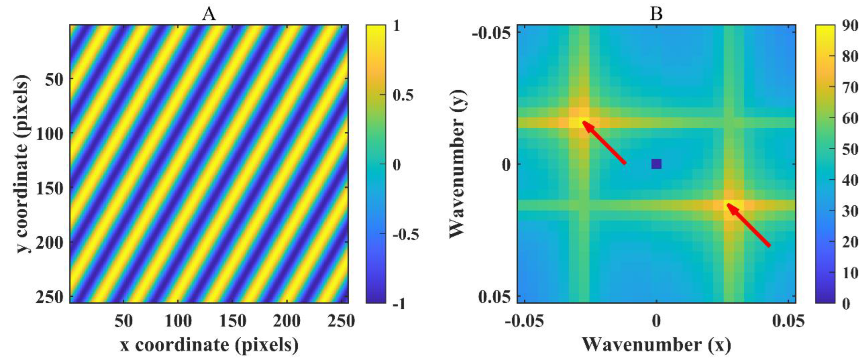
Figure 2.
Schematic diagram of spectral leakage suppression mechanism by truncating distorted pixel values: distorted pixel distribution (A) and its spectral energy analysis result (D); GMM fitting of distorted pixel values (B), where the gray bars represent the histogram of pixel counts, the black, red, and blue lines denote the Gauss mixture fit, the primary component, and the secondary component, respectively, and the green dashed lines indicate the upper and lower limits for pixel truncation; pixel distribution after truncation (C) and its spectral energy analysis result (E).
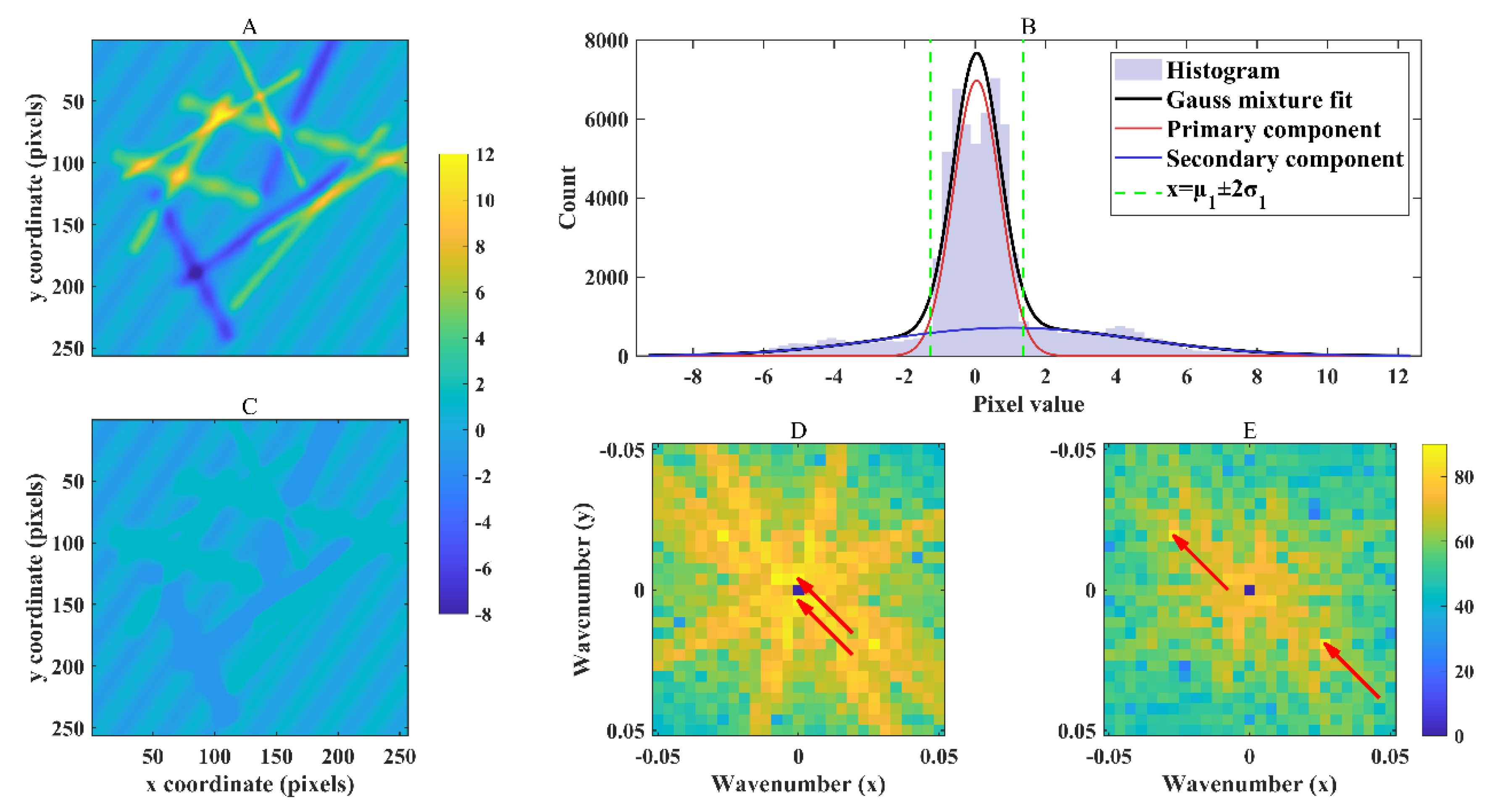
Figure 3.
Schematic diagram of the spectral leakage suppression mechanism by pixel detrending: pixel distribution containing a trend surface (A) and its spectral energy analysis result (B); fitted trend surface (C) and its spectral energy analysis result (D).
Figure 3.
Schematic diagram of the spectral leakage suppression mechanism by pixel detrending: pixel distribution containing a trend surface (A) and its spectral energy analysis result (B); fitted trend surface (C) and its spectral energy analysis result (D).
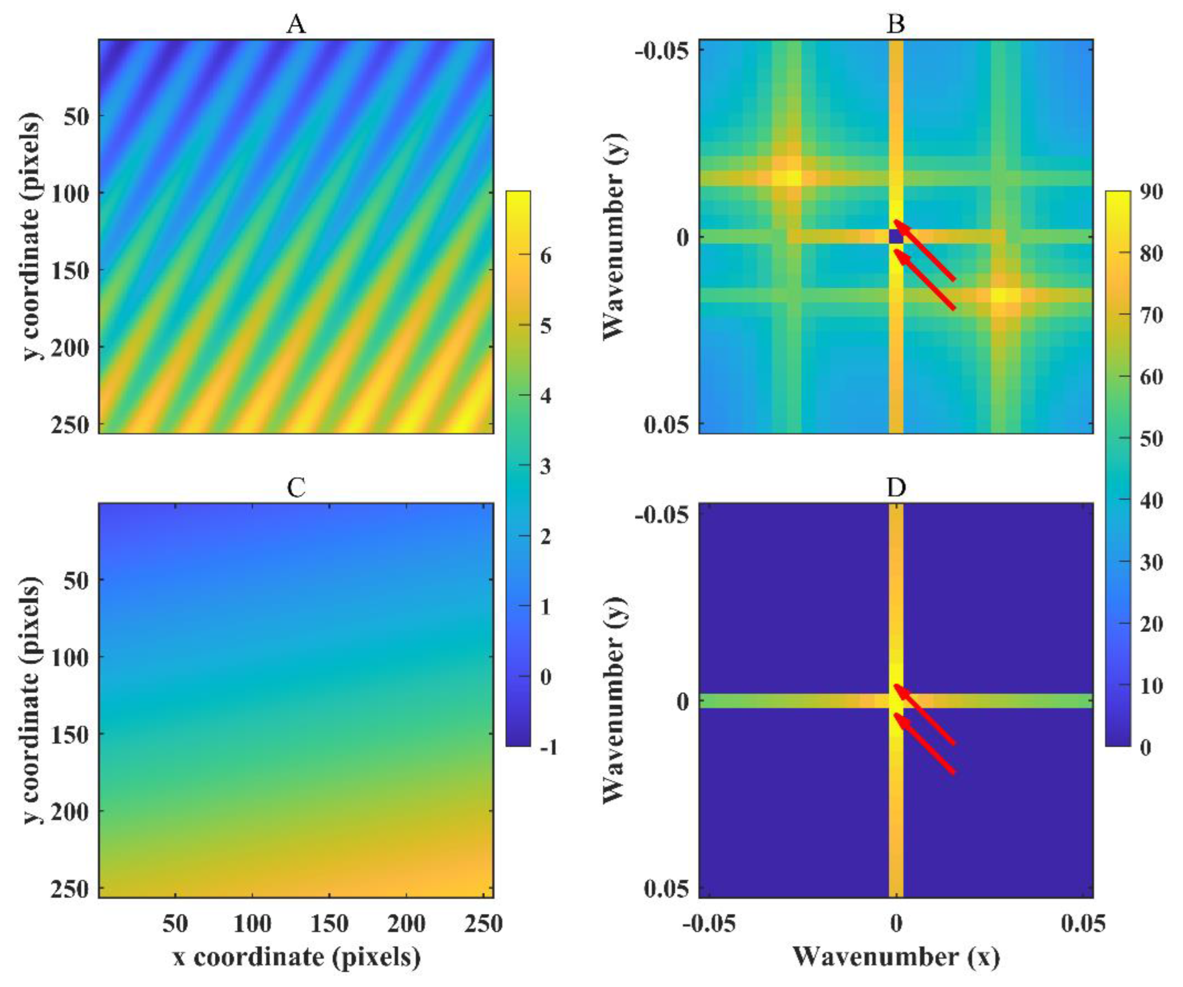
Figure 4.
Schematic diagram of the spectral leakage suppression mechanism by using the windowing technique: pixel distribution with edge discontinuities (A) and its spectral energy analysis result (B); pixel distribution after applying the window function (C) and its spectral energy analysis result (D).
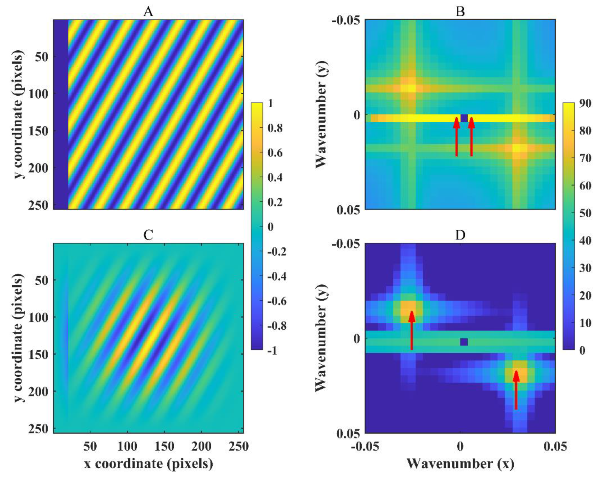
Figure 5.
WorldView-2 imagery (A) and nautical chart bathymetry (B) of the study area. Boxes 1-3 in Panel A mark the selected subimages exhibiting spectral leakage characteristics.
Figure 5.
WorldView-2 imagery (A) and nautical chart bathymetry (B) of the study area. Boxes 1-3 in Panel A mark the selected subimages exhibiting spectral leakage characteristics.
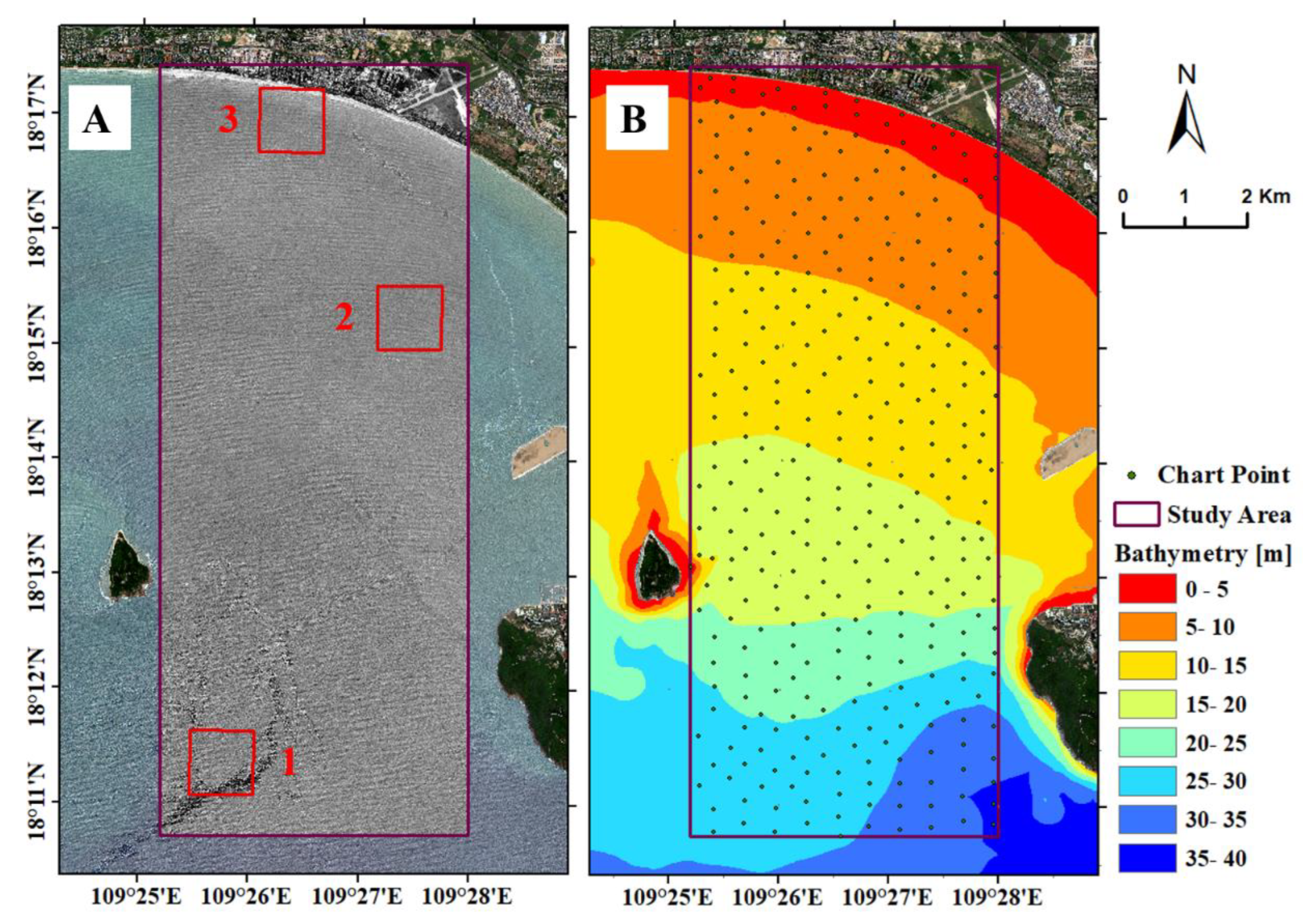
Figure 6.
Wavelength retrieval results from remote sensing imagery: (A) without spectral leakage suppression; (B) with suppression by truncation of distorted pixel values; (C) with suppression by detrending; (D) with suppression by windowing; (E) with combined suppression.
Figure 6.
Wavelength retrieval results from remote sensing imagery: (A) without spectral leakage suppression; (B) with suppression by truncation of distorted pixel values; (C) with suppression by detrending; (D) with suppression by windowing; (E) with combined suppression.
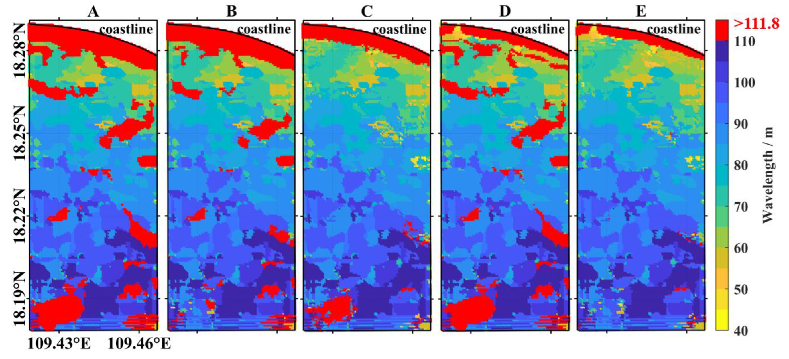
Figure 7.
Representative subimage illustrating spectral leakage suppression by truncation of distorted pixel values: (A) original pixel distribution; (B) corresponding spectral energy distribution; (C) pixel distribution after truncation; (D) corresponding spectral energy distribution after truncation.
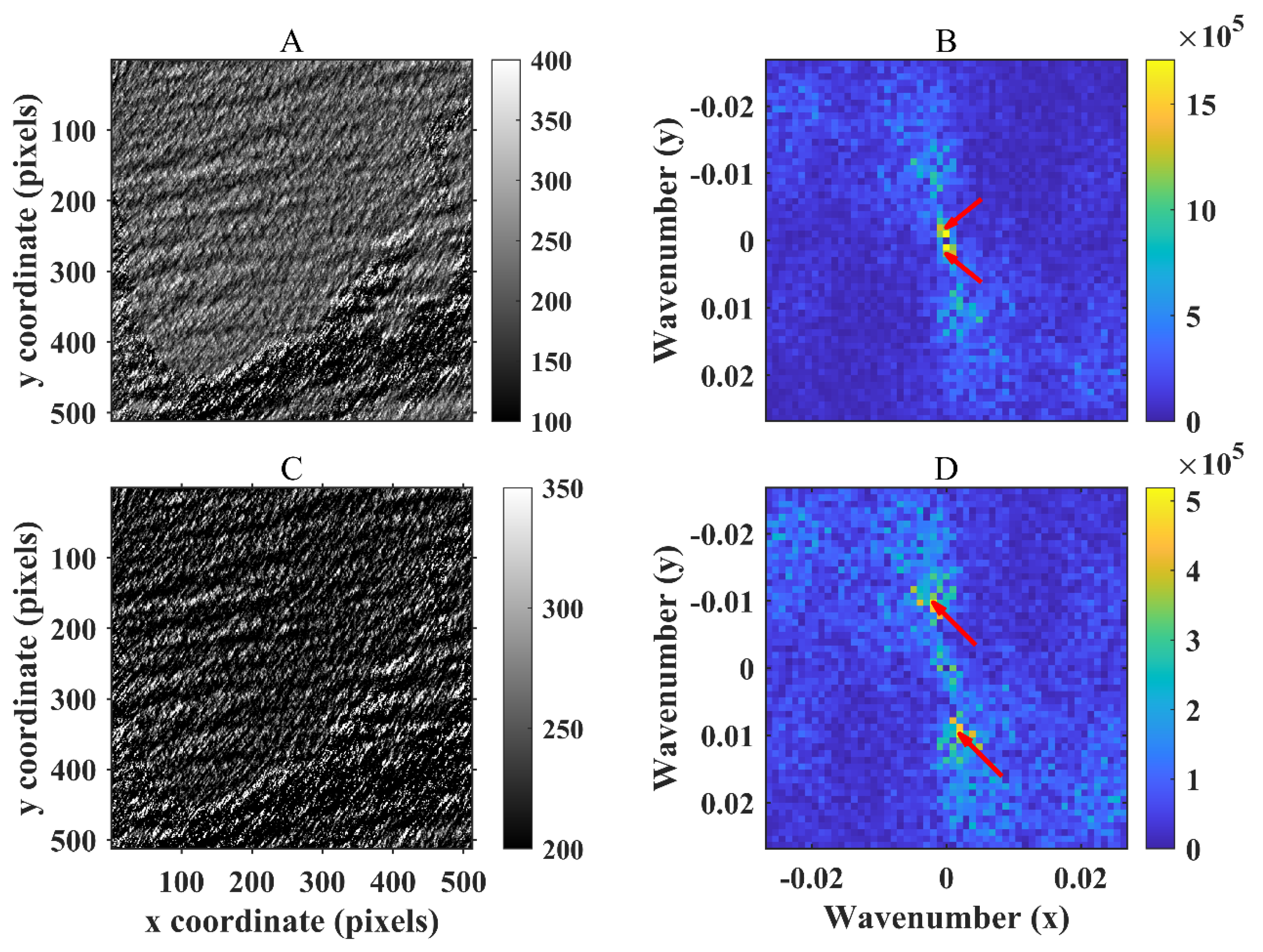
Figure 8.
Representative subimage illustrating spectral leakage suppression by pixel-value detrending: (A) original subimage; (B) corresponding energy spectrum showing maximum energy at low wavenumbers; (C) subimage after detrending; (D) corresponding energy spectrum after detrending, with maximum energy shifted to higher wavenumbers; (E) fitted trend surface.
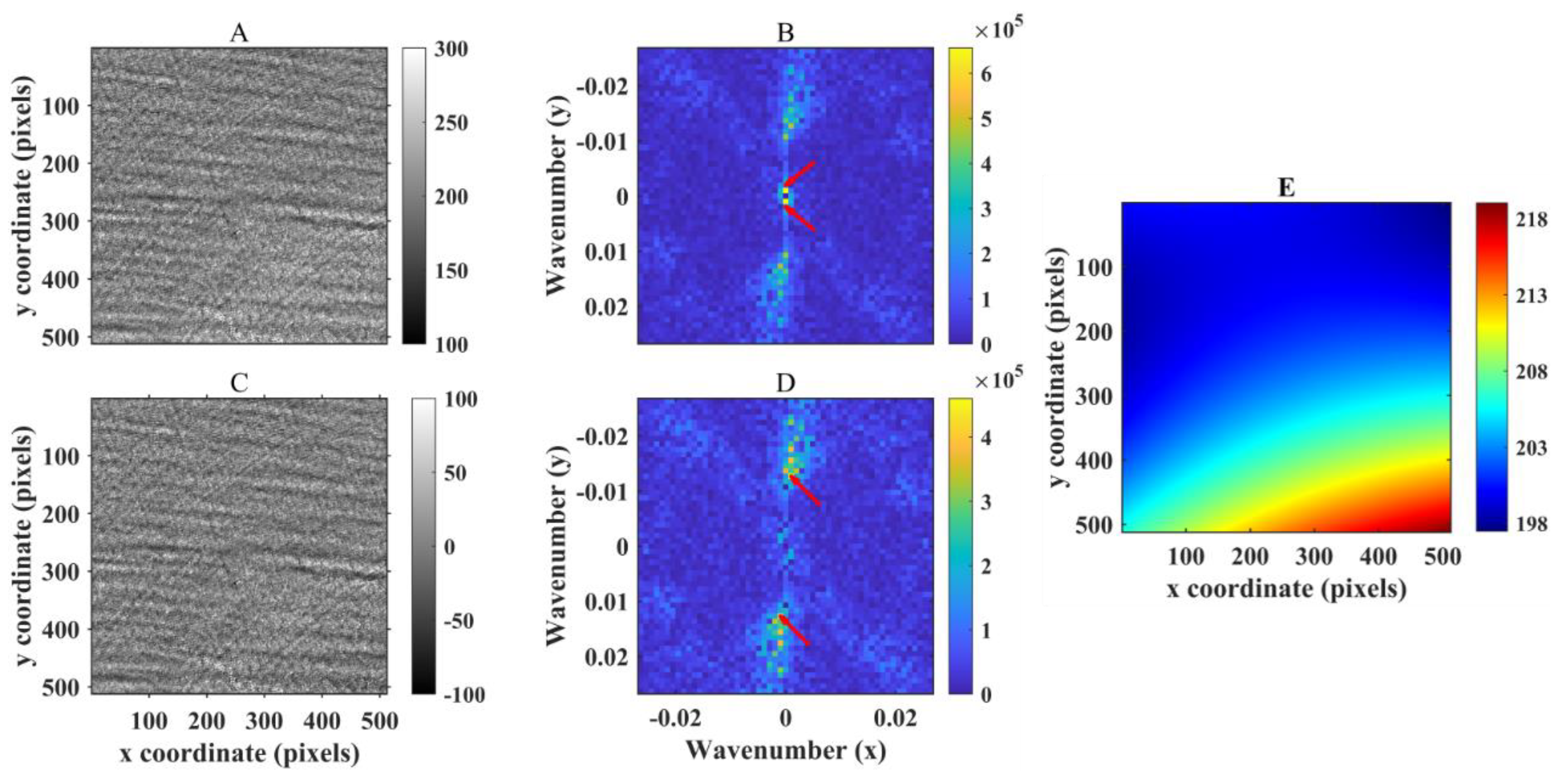
Figure 9.
Representative subimage demonstrating spectral leakage suppression by windowing in remote sensing imagery: original subimage (A) and its spectral energy analysis results (B); windowed subimage (C) and its spectral energy analysis results (D).
Figure 9.
Representative subimage demonstrating spectral leakage suppression by windowing in remote sensing imagery: original subimage (A) and its spectral energy analysis results (B); windowed subimage (C) and its spectral energy analysis results (D).
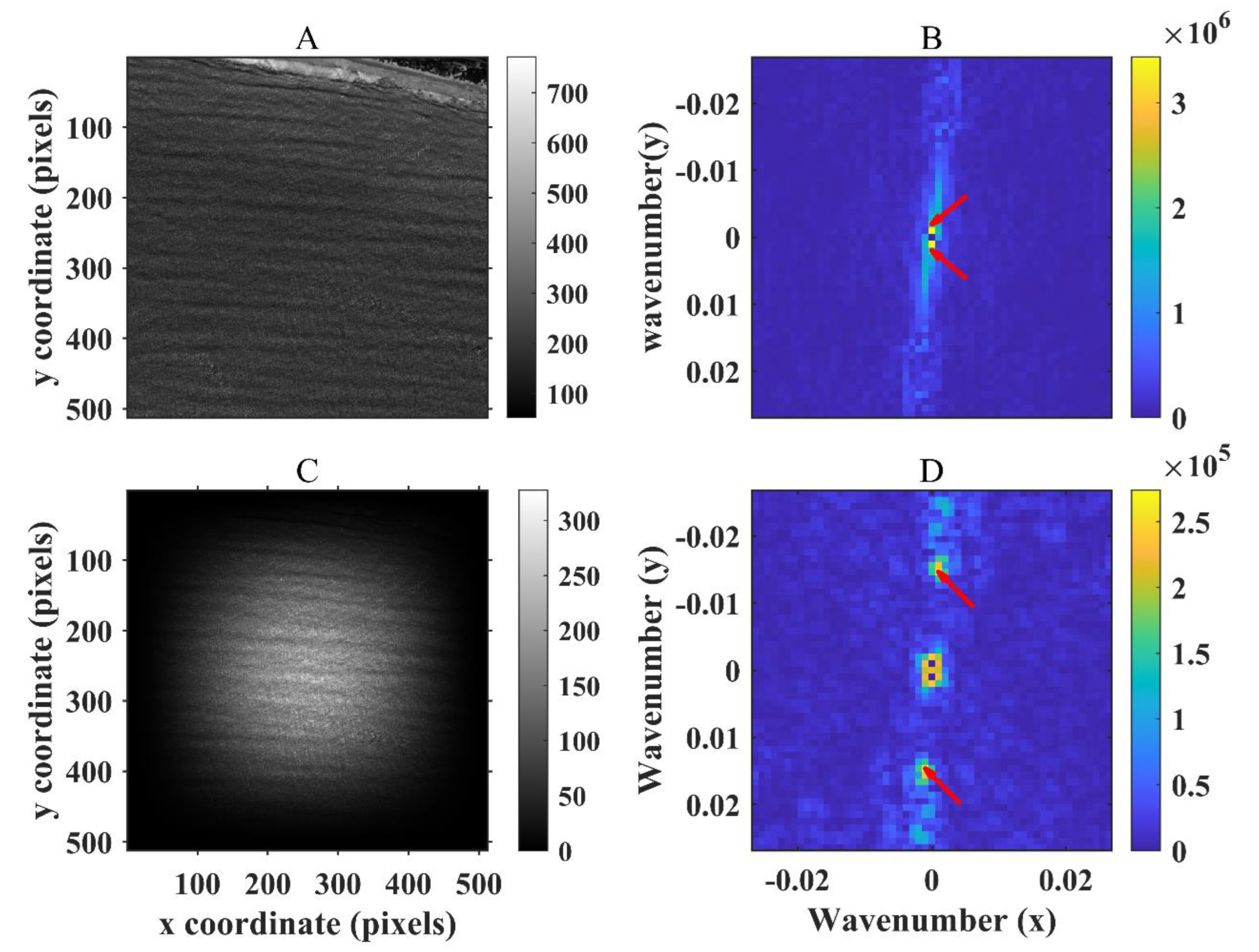
Figure 10.
Wave-derived bathymetry results from remote sensing imagery (A); comparison between retrieved depths from all subimages and chart soundings (B); comparison between retrieved depths from spectral-leakage-suppressed subimages and chart soundings (C).
Figure 10.
Wave-derived bathymetry results from remote sensing imagery (A); comparison between retrieved depths from all subimages and chart soundings (B); comparison between retrieved depths from spectral-leakage-suppressed subimages and chart soundings (C).
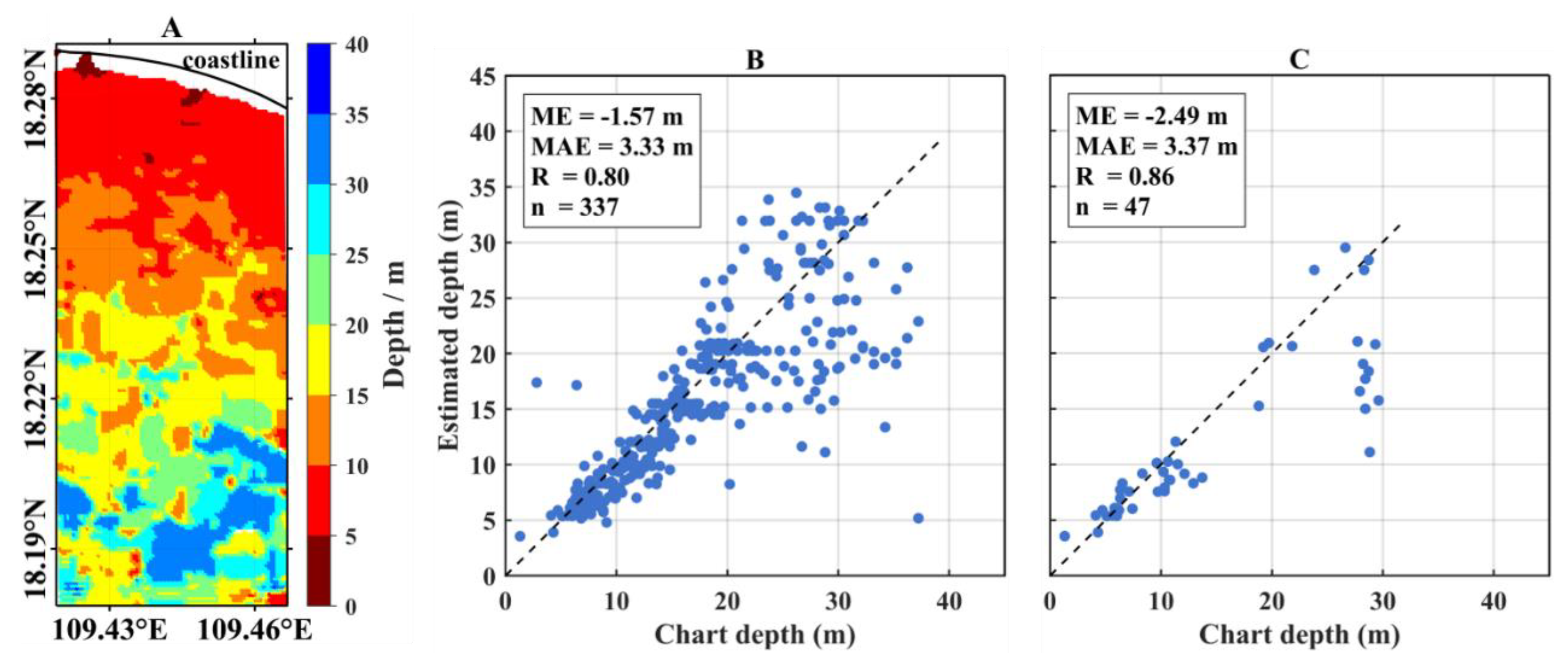
Figure 11.
Wavelength retrieval results from remote sensing imagery with different subimage sizes. Panels A–E: results for a subimage size of 512m, including (A) without spectral leakage suppression, (B) with distortion truncation, (C) with detrending, (D) with windowing, and (E) with combined suppression. Panels F–J: corresponding results for a subimage size of 2048m.
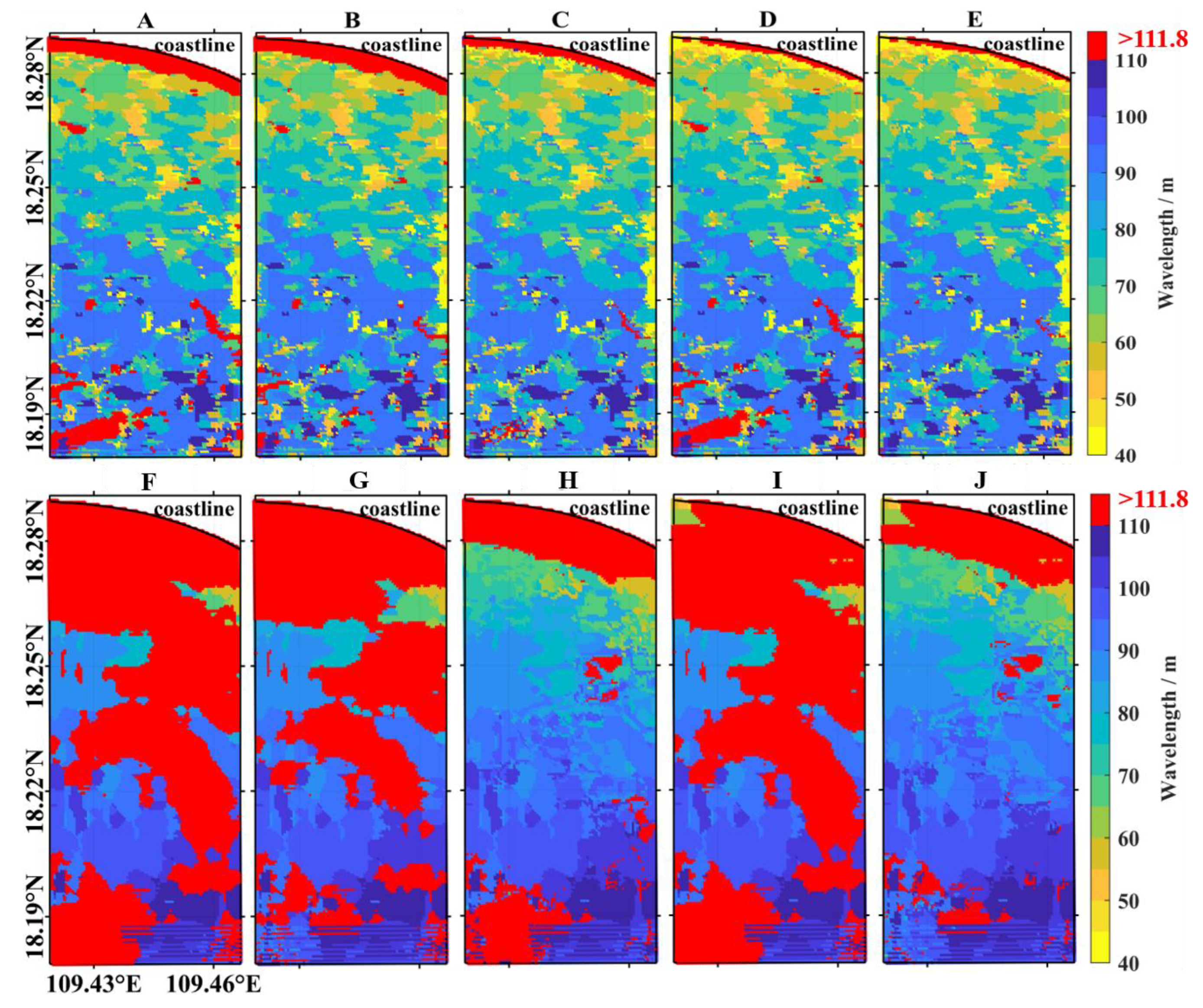
Figure 12.
Wave-derived bathymetry results with different subimage sizes. Panels A–C: results for a subimage size of 512m, including (A) inverted depths, (B) comparison between bathymetry from all subimages and chart data, and (C) comparison between bathymetry from spectral leakage–suppressed subimages and chart data. Panels D–F: corresponding results for a subimage size of 2048m.
Disclaimer/Publisher’s Note: The statements, opinions and data contained in all publications are solely those of the individual author(s) and contributor(s) and not of MDPI and/or the editor(s). MDPI and/or the editor(s) disclaim responsibility for any injury to people or property resulting from any ideas, methods, instructions or products referred to in the content. |
© 2025 by the authors. Licensee MDPI, Basel, Switzerland. This article is an open access article distributed under the terms and conditions of the Creative Commons Attribution (CC BY) license (http://creativecommons.org/licenses/by/4.0/).
Copyright: This open access article is published under a Creative Commons CC BY 4.0 license, which permit the free download, distribution, and reuse, provided that the author and preprint are cited in any reuse.


