
Submitted:
07 June 2025
Posted:
09 June 2025
You are already at the latest version
Abstract
Fixed automated (unmanned) above-water radiometric measurements are subject to unavoidable sky conditions and surface perturbations, leading to significant uncertainties in retrieved water surface remote sensing reflectances (Rrs(), sr-1) retrieval methods. This study evaluates various above-water Rrs() glint correction methods using a comprehensive dataset collected at the Royal Netherlands Institute for Sea Research (NIOZ) Jetty Station located in the Marsdiep tidal inlet of the Dutch Wadden Sea, the Netherlands. The dataset includes in-situ water constituent concentrations (2006–2020), inherent optical properties (IOPs) (2006–2007), and automated hyperspectral measurements collected every 10 minutes (2006–2023). The bio-optical models were validated using in-situ IOPs and utilized to generate glint-free remote sensing reflectances, Rrs,ref(), using a robust IOP-to-Rrs forward model. The Rrs,ref() spectra were used as a benchmark to assess the accuracy of glint correction methods under various environmental conditions, including different sun positions, wind speeds, cloudiness, and aerosol loads. The results indicate that the three-component (3C) reflectance model outperforms other methods across all conditions, producing the highest percentage of high-quality Rrs spectra with minimal errors. Methods relying on fixed or lookup-table-based glint correction factors exhibited significant errors under overcast skies, high wind speeds, and varying aerosol optical thickness. The study highlights the critical importance of surface-reflected skylight corrections and wavelength-dependent of glint estimations for accurate above-water Rrs retrievals. Two showcases on chlorophyll-a and total suspended matter retrieval further demonstrate the superiority of the 3C model in minimizing uncertainties. The findings highlight the importance of adaptable correction models that account for environmental variability to ensure accurate Rrs() retrieval and reliable long-term water quality monitoring from hyperspectral radiometric measurements.
Keywords:
Remote Sensing
; Water Quality
; Water Constituents
; Inherent Optical Properties
; Apparent Optical Properties
1. Introduction
Remote Sensing Reflectance (Rrs(λ), sr-1) is a crucial quantity in ocean color remote sensing tasks, which is necessary to develop water quality algorithms and evaluate the efficiency of the atmospheric correction algorithms [1,2,3]. In the field, Rrs(λ) is calculated as the ratio of water-leaving radiance (LW(λ), mW m-2 nm-1 sr-1) to downwelling irradiance (Ed, mW m-2 nm-1) just above the air-sea interface [4]. LW(λ) contains information of inherent optical properties (IOPs) such as absorption (a(λ), m-1) and backscattering (bb(λ), m-1) which are controlled by types and concentrations of Water Constituents Concentrations (WCCs) in the water column [5]. In-situ measurements of LW(λ) are challenging due to specular reflections caused by surface-reflected light causes on the water surface [6]. The skylight-blocked approach (SBA) method has been utilized to measure LW(λ) in the field. The SBA can measure LW(λ) with high precision across different water types, but it is susceptible to uncertainties caused by self-shading, floating structure, and marine bio-foaling [6,7,8]. In contrast, LW(λ) can be easily determined from above-water measurements using low-cost instruments and over long periods of time [9,10]. The above-water measurements include downwelling irradiance, upward radiance, and reflected sky radiance, which are measured simultaneously. In this way, the resulting LW(λ) is influenced by sensor viewing angle (θV), sensor viewing azimuth (φV), solar zenith angle (θS), solar azimuth (φs), wind-induced surface roughness, and sky conditions (e.g., cloudiness) [4,11,12]. Both above and in-water measurements have their advantages and disadvantages for accurate estimations of Rrs(λ) [13,14]. In the following, we focus on above-water measurements.
Automated above-water hyperspectral radiometry in a fixed station is a cost-effective solution that provides long-timeseries of measurements. This type of measurement records the solar planar downwelling irradiance (Ed(λ), mW m-2 nm-1), and sky (LS(λ), mW m-2 nm-1 sr-1) and surface (LT(λ), mW m-2 nm-1 sr-1) radiances in short time steps (i.e., minutes or seconds) simultaneously. However, atmospheric conditions have a significant impact on Ed(λ) and LS(λ), and water surface roughness affects the LT(λ). Both factors introduce considerable uncertainty to Rrs(λ). To overcome this problem, researchers have developed various methods, which can be estimated through bio-optical modelling [15,16] or through a similarity spectrum approach [17]. In this way, Rrs(λ) is calculated from simultaneous measurements of ES, LS, and LT as follow [4,18]:
where the geometry factor of (θv, Δφ) indicates the directions seen by radiometer. ρ(θv,Δφ) (dimension less, dl) is the effective surface reflectance that rescales the sky radiance to the reflected sea surface radiance. It is assumed that it is independent of the wavelength [4,19,20,21] or dependent on the wavelength [2,22,23]. ΔL (sr-1) is the reflectance offset due to the total glint contribution and/or variabilities of Ed(λ) and LS(λ) that are not consistent with LT(λ). For flat surface, ρ(θv, φV) equals the Fresnel reflectance of the sea surface. Various approaches have been suggested for estimating ρ, including: fixed ρ values [20,24,25], sky-conditions dependent ρ values [26], lookup tables of ρ(θv,Δφ) for various directional factors and wind speed [4,27], and wavelength-dependent of ρ(λ,θv,Δφ) for various directional factors, wind speeds, and aerosol loads [22]. However, a sensor geometry with θv = 40° and φ = 90°−135° is considered optimal to minimize glint perturbations [4], so in practice these geometries are usually fixed. Similarly, researches have considered different approaches to estimate the ΔL estimation, including a fixed value equal to the Rrs(λ) at Near Infra-Red (NIR) [28,29,30,31], values of the similarity spectrum at NIR [17], the difference between bio-optical models and simulated Rrs(λ) [15], and estimating the direct surface reflected radiance to simulate ΔL [19,21]. The last approach substitutes a wavelength-dependent correction factor of ΔL(λ) in Equation (1). Since automated above-water radiometry is subject to unavoidable varying environmental conditions, application of above-water radiometric measurements introduces additional challenges. Consequently, there is a need for a thorough review and assessment of methods because the estimates ρ and ΔL may not be accurate enough for long timeseries of measurements in all environmental conditions.
The analytical methods for deriving IOPs from Rrs(λ) comprise inverse modeling that cannot be exactly reduced to an analytical equation or expression and relies on empirical and/or semi-empirical relationships [32]. However, The Radiative Transfer (RT) simulations and the quasi-single scattering approximation (QSSA) forward models have been developed to estimate Rrs(λ) as a function of spectral IOPs [5]. Several forward QSSA analytical expressions have been developed that estimate the Rrs(λ) as a function of a(λ), m-1) and bb(λ) [5,33,34]. Similarly, RT models simulate Rrs(λ) as a function of user-input IOPs and environmental parameters [4,33,35]. Therefore, RT and QSSA forward models explicitly relate IOPs to Rrs(λ) free of sun and sky glint. The resulting Rrs(λ) can be used as a reference to evaluate the above-water Rrs(λ) from Equation (1). In this regard, the lack of IOPs is a critical factor that significantly impacts the outcomes of this study. The validated regional bio-optical models can be utilized to overcome the lack of IOPs data [5].
This research aims to evaluate the performance of various sun, sky, and surface glint correction models from a fixed automated above-water radiometric measurements in highly turbid coastal waters. We will assess the strengths and limitations of the proposed models in various environmental conditions. Finally, we provide two showcases to further confirm the significance of the total glint correction models for above-water radiometry.
2. Field Data
2.1. Above-Water Hyperspectral Radiometric Data
We utilized a time-series of above-water hyperspectral measurements spanning from 2006-2023 at the Royal Netherlands Institute for Sea Research (NIOZ) jetty station (NJS) located near the Marsdiep tidal inlet of the Dutch Wadden Sea (Figure 1a). NJS has been equipped with a set of 6 TRIOS-RAMSES radiometers, comprising 1 Ramses-ACC for measuring solar downwelling irradiance (Ed, mW m-2 nm-1), 1 Ramses ACC-UV for measuring solar downwelling irradiance in the ultraviolet region (ES-UV, mW m-2 nm-1), 2 pairs of Ramses-ARC for measuring sky radiance (LS, mW m-2 nm-1 sr-1), and total upwelling radiance from water surface (LT, mW m-2 nm-1 sr-1). The spectral data was recorded every 10 minutes at 1 nm intervals, ranging from 350 nm to 950 nm. The ARC sensors were set up with viewing angle θV = 35° and direction φV = 135° (south-east) and φV = 225° (south-west) (Figure 1b–d). A set of quality control tests were applied to the hyperspectral data to flag the invalid or suspicious spectra [36]. The quality-controlled flagged spectra were excluded from further analysis. In this study, we used the quality-controlled Ed(λ), LS(λ), and LT(λ) covering 6:00 AM to 6:00 PM (UTC).
2.2. Meteorological Data
Hourly meteorological observations from the De Kooy station (Figure 1), located approximately 8 km southwest of NJS, covering the period from 2006-2023, were obtained from The Royal Netherlands Meteorological Institute (KNMI) database (https://dataplatform.knmi.nl). Measurements included cloud cover (CC, coverage of the upper sky in eighths, with ‵9‵ indicating the upper sky invisible), atmospheric pressure (hPa), relative humidity (%), and wind speed (m s-1).
2.3. IOPs Data
Reference [25] measured IOPs at 156 stations across the entire Wadden Sea between 2006 and 2007. Of these, 22 stations collected at NJS during March, June, and July 2006, were used in this study (hereafter referred to HA09). The HA09’s IOPs dataset included laboratory spectrophotometry of total absorption (a(λ), m-1), Colored Dissolved Organic Matter (CDOM) absorption (aCDOM(λ), m-1), particle absorption (ap(λ), m-1), Non-Algal Particle (NAP) absorption (aNAP(λ), m-1), and phytoplankton absorption (aPhy(λ), m-1). They have measured particle absorption with a spectrophotometer (Ocean Optics) using the filter pad method. In addition, beam attenuation (c(λ), m-1) and total absorption were measured in-field using an AC9 (Wet Lab, 25 cm cuvette, linearity range 0.001-30 m-1), hereafter cAC9(λ) and aAC9(λ). The AC9 operated at nine standard wavelengths (412, 440, 488, 510, 555, 630, 650, 676, and 750 nm) ([25], their table 2). Both in-situ and ex-situ measurements were conducted based on standard protocols [37], corrected for blank measurements on MilliQ water, and corrected for temperature-salinity and scattering [38], respectively. Only the AC9 data at depth ≤ 1.0 m were utilized, along with spectrophotometer data. The particle scattering was calculated as bp(λ) = cAC9(λ) - aAC9(λ) for in-situ AC9 data. The light backscattering coefficients of particles were determined as follow [35,39]:
where B is the backscattering probability (or backscattering ratio), assumed to be spectrally constant [40,41]. The values of B ranged between 0.024 to 0.042 for surface waters of the coastal area of the English channel [42]. The value of B has been assumed to be 0.026 in the Wadden Sea (Please see supplementary, Section S1).
The HA09 dataset also included supplementary in-situ data of wind speed (m s-1), water temperature (C°), Ph, salinity (PSU), Secchi Disk Depth (SDD, m-1), and wave height (m).
2.4. Concentrations of Chla and SPM
A total of 1015 surface water samples were collected at NJS during 2006-2020 for laboratory Chla and Suspended Particle Matter (SPM, g m-3) measurements. Of these, 648 samples included measurements of both Chla and Total Suspended Matter (TSM, g m-3). The Chla concentrations of the NJS dataset included two groups of High-Performance Liquid Chromatography (HPLC) and Fluorometry measurements. The Chla concentrations of HA09 and NJS-HPLC samples were measured using standard HPLC measurements on samples filtered through GF/F filters then frozen and transported to laboratories for analysis. The Chla concentrations of NJS-Fluorometry samples were measured using a laboratory Fluorometer on filtered samples using standard methods by 43]. TSM concentrations were measured using the standard filtration method described by [37] using pre-ashed, rinsed, and weighted 47 mm GF/F filters. Readers are referred to [25,24] for more details on these measurements.
3. Methods
Since the temporal coverage of measured IOPs was limited to HA09 datasets, the bio-optical models were used to simulate the IOPs using the average of HA09 dataset and measured WCCs at NJS. Subsequently, the Rrs(λ) from above-water radiometric measurements were evaluated against glint-free Rrs(λ) simulated using IOP-to-Rrs(λ) forward models.
3.1. Bio-Optical Models
IOPs are expressed as the sum of absorption or scattering by water molecules and various dissolved and particulate water components [44]. CDOM, NAP, and phytoplankton are the representative of the natural water particles with distinct absorption and backscattering. The total absorption (a(λ), m-1) and backscattering (bb(λ), m-1) coefficients of water can be expressed as follows [1,45]:
where the subscripts w, Phy, CDOM, and NAP present contributions by pure water, phytoplankton, CDOM, and NAP constituents. Since CDOM backscattering is negligible, it is left out in Equation (4). The total non-water absorption (anw, m-1) and particulate backscattering (bbp, m-1) are expressed as the sum of the non-water constituents: , . Table 1 summarizes the algorithms for parameterizing absorption and backscattering of phytoplankton, CDOM, and NAP in coastal waters.
In this study, the absorption coefficients of water constituents were calculated (Eqs. 5-9) and the results were validated using the HA09 field measurements. The spectral slope of CDOM (SCDOM, nm-1) and NAP (SNAP, nm-1) were calculated by fitting the exponent of aCDOM between 350-500 nm and 380-730 nm, respectively [54]. To calculate SNAP, the aNAP(λ) in the 400-480 nm and 620-710 nm ranges were excluded to avoid pigment absorption residuals [54,55]. The absorption of pure water, aw(λ), was taken from [56,57] in the ranges of 350-550 nm and 555-700 nm, respectively. According to Table 1, anw(λ) was calculated in two ways, one using the sum of Eqs. 6, 8, and 9 (anw,BR19x(λ) hereafter) and the other using the sum of Eqs. 7, 8, and 9 (referred to anw,LC99(λ) hereafter).
Reference [24,28] utilized the parametrization of bb(λ) using Eqs. 10 and 12 to retrieve the WCC at the NJS. They showed that the measured SIOPs by [25] were valid for WCC retrieval. Therefore, we used the same parametrization for the backscattering model (bb,BA18(λ) hereafter). In addition, we tested the parametrization of bb(λ) using Equations (11) and (13) (bb,GE05(λ) hereafter). The backscattering coefficient of pure water (bb,w(λ)) was obtained from [39].
The Specific IOPs (SIOPs) (denoted by * in Table 1) were calculated as:
a*Phy(λ) = aPhy(λ)/Chla (m2 mg-1), b*SPM(λ) = bbp(λ)/SPM (m2 g-1) , and a*NAP(λ) = aNAP(λ)/SPM (m2 g-1). Table 2 shows the statistical ranges of WCCs, absorption, and backscattering used for bio-optical model parametrization.
3.2. Generating the Glint-Free Rrs(λ)
The bio-optical models were used to obtain glint-free Rrs(λ). The bio-optical model could be represented as follows [58,59,60]:
where α and β are constant values retrieved from a lookup table based on θv, Δφ, θs, wind speed, and cloud cover presented in [35]. The gw and gk are the model parameters dependent on θS and sensor geometry, retrieved from a lookup table presented by [59]. This model has been used for high sediment load waters [59,61]. Equation (14) model was used to generate the glint-free Rrs(λ) spectra (Rrs,ref(λ) hereafter) using the average IOPs and measured WCCs.
3.3. Methods of ρ and ΔL Estimation from Above-Water Radiometry
In this study, the determination of ρ(θv,Δφ) and ΔL have been considered using methods presented in Table 2. Table 3 summarizes the methods of estimating the ρ(θv,Δφ) and ΔL factors. Regarding the ρ, the models were categorized into 4 groups, including: i) fixed values of ρ(θv,Δφ), ii) lookup tables for wind speed and sun-sensor geometries, iii) wavelength-dependent approaches and dependency of Aerosol Optical Thickness (AOT), wind speed, and sun-sensor geometries (HT23 and ZX17), and iv) using direct measurements of radiometric data. The Ku13 and JD20 models are not sensitive to the ρ(θv,Δφ) value, as they primarily focus on the shape of the water surface reflectance spectra. The ZX17 presents a lookup table of simulated ρ(λ) as a function of AOT, θs ≤ 60°, wind speed, and sun-sensor geometries in clear skies.
Since environmental conditions were not specifically considered in the models, we evaluated the performance of selected models in various environmental conditions, including sky cloudiness and AOT loads. The viewing geometry (θv,Δφ) and wavelength (λ) were omitted for brevity hereafter. In addition, the quality of Rrs(λ) was used to evaluate the results of models in different conditions using the Quality Assurance (QA) scores provided by [62]. The QA scores ranged from 0 (invalid) to 1 (perfect).
3.4. Identification of Environmental Factors
The environmental factors used in the previous sections were obtained as follows:
3.4.1. Sun Azimuth and Zenith Angle
The θS and φS were calculated for the date-time of observations using the method presented in the “Climate Data Toolbox” [63].
3.4.2. Aerosol Optical Thickness (AOT)
A spectrum of Ed(λ) is a sum of the direct and diffusive components of downwelling irradiance, which can be calculated based on the Gregg and Carder model (GC90 hereafter) [64]. The GC90 model has been developed primarily for cloudless maritime atmospheres. The RADTRAN solar irradiance model [65] has been developed based on the GC90 along with the use of spectral cloud transmission based on the delta-Eddington approximation of two-stream approach flowing Slingo [66]. An R-based implementation of this model is available at https://rdrr.io/github/sean-rohan-NOAA/trawllight/man/radtran.html. In this study, the direct and diffusive components of solar irradiance were calculated using the inverse RADTRAN model of Ed(λ) using the parametrization provided by [16] and corresponding meteorological data. Subsequently, AOT was calculated using the Ed(λ), direct and diffuse solar irradiance following the methods presented by [67].
The AOT(550) values were in the range of 0.01 to 1.2. In general, AOT(550) was found to be approximately 0.1 for clear atmospheres, 0.4 for moderately turbid atmospheres, and greater than 1.0 for very turbid atmospheres [22]. Here, we considered the AOT(550) ≤ 0.1 as ‘low AOT’, and AOT(550) ≥ 0.5 as ‘high AOT’ atmospheric conditions.
3.4.3. Sky Conditions (Clear, Scattered Clouds, or Overcast)
We have developed a method for identifying sky conditions as a function of cloudiness using hyperspectral observations of Ed(λ) and LS(λ). This methods is based on the work of [68] that utilizes the spectral solar irradiance model developed by [64] for cloudless maritime atmospheres. Specific criteria were established to identify cloud presence based on time series data of Ed(λ) at 550 nm. This model differentiated cloudless skies, scattered clouds, and overcast conditions using RT simulations. The details of this method is available in [36]. Here, the hyperspectral data were collected over a broad range of environmental conditions, encompassing clear (11.8% of observations) and cloudy skies, low to high sun zenith angles (28-89°), and low to high wind speeds (1-14 m s-1).
3.5. Statistical Metrics
The statistical parameters of standard deviations (std), normalized Root Mean Square Error (NRMSE), coefficient of determination (R2), Mean Absolute Percentage Error (MAPE), Unbiased Percentage Difference (UPD), normalized mean difference or bias (NBias), and mean ratio (MR) were used to quantify the consistency between models and observations.
where xmod and xobs represent the estimated and observed values, n is the number of observations. A statistical score was defined based on the values of NRMSE, MAPE, UPD, and R2 as follow [69]:
where the subscript ‘nor’ indicates statistical normalization = [x – min(x)]/[max(x) – min(x), and Wx is the weight of each parameter, assigned an equal value of 0.25 for each parameter. The Total Score varies between 0 to 1, with higher values for higher statistical consistency between observed and modeled parameters.
4. Results
4.1. Parametrization and Validation of Bio-Optical Models
The bio-optical models are parametrized using the average values of measured a*Chl(λ), aCDOM(λ2), a*NAP(λ), SCDOM, SNAP, b*SPM(λ), and WCCs (Table 2). The normalized aPhy(λ) shows low variability (CV = 0.06 at 410 nm and CV = 0.03 at 675 nm) indicating phytoplankton remain relatively consistent during the measurements. The normalized aCDOM(λ) and aNAP(λ) spectra for the entire dataset show a minimal difference across the spectral structure. As a result, the mean values of a*Phy(λ), aCDOM(λ2), aNAP(λ), SCDOM and SNAP are used for parametrization of the absorption models in Eqs. 6, 8, and 9 (Table 3). Moreover, the mean values of b*SPM(λ) = bSPM(λ) / [SPM] m2 g-1 are used for the parametrization of the NAP backscattering coefficient (Equation (12)). Figure 2 shows the correlations between the measured and estimated absorption and backscattering coefficients. The values of MAPE, NRMSE, NBias, MR, and R2 of aPhy(λ) from Equation (6)\(7) against in-situ measurements are 15.0\24.2%, 0.15\0.26, 0.02\0.03, 0.88\0.75, and 0.91\0.84, respectively. The measured aPhy(λ) spectra exhibit more consistency with the spectra calculated from Equation (6) than Equation (7). The exponential fits of aCDOM(410) and aNAP(410) show very good consistency with measurements (MAPE ≤ 3.6%, NRMSE ≤ 0.06, NBias ≤ 0.03, MR ≅ 1.0, and R2 ≥ 0.95). The correlation between in-situ anw(440) and anw,BR19x(440) shows more consistency with measurements than anw,LC99(440) (MAPE = 4.3%, NRMSE = 0.11, NBias = 0.04, MR = 0.98, and R2 = 0.86). Therefore, parametrization of Equation (3) using ap,BR18x(λ) (Equation (6) + Equation (8) + Equation (9)) represents the optimum setup that correlates well with the in-situ measurements. Parametrization of bbp(λ) using bb,GE05(440) components show more consistency than those by bb,BA18(440), with the values of MAPE = 18.8 & 23.8%, NRMSE = 0.12 & 0.16, NBias = 0.03 & 0.04, MR = 0.89 & 0.83, and R2 = 0.92 & 0.87, respectively. All estimated IOPs fall within the boundaries of the 95% confidence level of the measurements. The findings indicate that the HA09 average SIOPs are valid for bio-optical model applications.
4.2. Evaluation of ρ and ΔL Estimation Methods
The Rrs,ref(λ) are calculated using Equation (14) utilizing the average of SIOPs (Table 2) and measured WCCs for the time periods when in-situ measurements are available. The Rrs(λ) spectra corresponding to the Rrs,ref(λ) are calculated using the quality-controlled Ed(λ), LS(λ), and LT(λ) spectra from south-east and south-west looking sensors base on the proposed methods outlined in Table 3. Figure 3 shows the average of modeled Rrs(λ) and Rrs,ref(λ) spectra in various environmental conditions. The corresponding error estimates of each case in terms of statistical Total Score (Equation (21)) between Rrs(λ) and Rrs,ref(λ) are shown in Figure 4. The full set of statistical parameters comparing Rrs(λ) and Rrs,ref(λ), and associated scatter plots are shown in the Supplementary Material Figures S1–S4. The environmental conditions are defined as follows.
Case I, high Δφ: Clear skies, θS ≤ 45°, wind speed ≤ 3 m s-1, low AOT, and Δφ ≥ 60° (Figure 3a and Figure 4a). (N = 65). This case is characterized by low variability of Rrs(λ) spectra. The lowest deviations from Rrs,ref(λ) are achieved by 3C model (Total Score = 0.90, MAPE = 8.8%, UPD = -2.4, NRMSE = 16.1%) in the range of 400-720±5 nm, and the heist deviations by the Ru05 (Total Score = 0.76, MAPE = 32.9%, UPD = -9.7, nRMSE = 24.7%). Similar results are found in the range of λ=440±5 nm (blue), λ=560±5 nm (green), λ=680±5 nm (red), and λ=720±5 nm (NIR). The other methods show intermediate and relatively similar error estimates against Rrs,ref(λ), with an average of Total Score = 0.79, MAPE = 19-28%, UPD = -8-7, and nRMSE = 24-28%.
Case II, low Δφ: Clear skies, θS ≤ 45°, wind speed ≤ 3 m s-1, low AOT, and Δφ ≤ 40° (Figure 3b and Figure 4b). (N = 83). This case is characterized by high deviations of the models that utilize lookup tables of ρ and BA18. The 3C model shows the best score with Total score = 0.91, MAPE = 8.7%, UPD = 2.9, and NRMSE = 15.8% in the range of 400-720±5 nm. Similar statistical results are observed for the blue, green, red, and NIR regions. The worst statistical scores are observed for MO99, MO15, BA18, HT23, and ZX17 methods with Total Score = 0.56, MAPE > 100%, UPD = -18, and NRMSE = 14-25%.
Case III, Overcast sky condition: Overcasts, 45° ≤ θS ≤ 65°, wind speed ≤ 3 m s-1, low AOT, and 40° < Δφ < 60° (Figure 3c and Figure 4c). (N = 115). The MO99, MO15, BA18, and HT23 show a significant overestimations against Rrs,ref(λ) across all wavelengths, with Total Score = 0.54, MAPE = 91-97%, UPD = -14.6- -14.8, NRMSE = 20-24%. The lowest deviation belongs to the 3C model with Total Score = 0.93, MAPE = 7.4%, UPD = 1.5, and NRMSE = 11.8%. The visual comparison shows that the Ku13 and JD20 models underestimate significantly Rrs(λ) in the blue and NIR regions. The ZX17 is not available for this case.
Case IV, scattered cloud condition: Scattered clouds, 45° ≤ θS ≤ 65°, wind speed ≤ 3 m s-1, low AOT, and 40° < Δφ < 60° (Figure 3d and Figure 4d). (N = 307). This case is characterized by high deviations and overestimations of MO99, MO15, BA18, and HT23 methods with Rrs(560) = 0.022-0.027 sr-1 and Total Score = 0.59, MAPE = 85-93%, UPD = -12.5 – 15.2, and NRMSE = 9.1-10.2%. The best simulation belongs to the 3C model with a Total Score of 0.92. The ZX17 is not available for this case.
Case V, strong wind speed: Clear skies, 45° ≤ θS ≤ 65°, wind speed ≥ 9 m s-1, low AOT, and 40° ≤ Δφ ≤ 60° (Figure 3e and Figure 4e). (N = 69). Visual comparison of Rrs(λ) spectra indicates the relatively high variability and underestimations in the blue wavelength regions by JD20 and Ku13 methods, which utilize spectral shape for corrections. The 3C & Ru05 show the best performance with Total Score = 0.90 & 0.79, MAPE = 8.8% & 17.3%, UPD = 1.4 & -6.3, and NRMSE = 17.3% & 24.3%, respectively.
Case VI, high wind speed: Clear skies, 45° ≤ θS ≤ 60°, 4 ≤ wind speed ≤ 7 m s-1, low AOT, and 40° ≤ Δφ ≤ 60° (Figure 3f and Figure 4f). (N = 211). This case is characterized by overestimation of the MO99, MO15, BA18, HT23, and ZX17 methods with an average of ΔRrs(560) = 0.009 sr-1 relative to Rrs,ref(λ), with Total Score = 0.58, MAPE = 92-98%, UPD = -16.8 - -16.1, and NRMSE = 9.8-11.2%. The 3C model shows the best performance with Total Score = 0.93, MAPE = 6.6%, UPD = 1.2, and NRMSE = 8.8%. The JD20 and Ru05 show the best performance next to the 3C model. The HT23 and ZX17 show similar result.
Case VII, high AOT: Clear skies, 45° ≤ θS ≤ 60°, wind speed ≤ 3 m s-1, high AOT, and 40° ≤ Δφ ≤ 60° (Figure 3g and Figure 4g). (N = 32). This case is characterized by low variability of Rrs(λ) spectra. All models except Ru05 underestimate the Rrs(λ) spectra with an average of ΔRrs(560) = 0.004 sr-1 relative to the Rrs,ref(λ) spectra in the blue and green regions. The Ku13 and JD20 methods show the highest deviations in the blue and green regions (UPD = 11.5-18.8, and NRMSE = 37.6-60.1%). The HT23 and ZX17 show a good performance in the green-red regions (Total Score = 0.89, MAPE = 9.5%) and a relatively weaker performance in the blue region (Total Score = 0.75, MAPE = 29.3%). Overall, the 3C model show the best performance, with Total Score = 0.89, MAPE = 9.3%, UPD = 4.6, and NRMSE = 19.1%.
Case VIII, high sun-zenith angle: Clear skies, θS ≥ 80°, wind speed ≤ 3 m s-1, low AOT, and 40° ≤ Δφ ≤ 60° (Figure 3h and Figure 4h). (N = 11). All methods show low variabilities. Apart from the 3C, the other methods underestimate the Rrs(λ) spectra in the blue-NIR regions. The MO99, MO15, Ru05, BA18, HT23, and JD20 show relatively similar performance with Total Score = 0.81-0.84, MAPE = 11.6-15.1%, UPD = -1.2- 4.6, and NRMSE = 30.1-32.4%. The Ku13 shows a very weak performance in the blue region with a Total Score of 0.36. The 3C model shows the best performance in this case with Total Score = 0.92, MAPE = 5.2%, UPD = 0.92, and NRMSE = 22.7%. The ZX17 is not available for this case.
4.3. Variability of ρ and ΔL
Figure 5a shows the variability of ρ values for the eight Cases. The ρ values are not highly sensitive to the environmental conditions and are in the range of 0.0271±0.0007 for MO99, 0.0309±0.0008 for MO15, 0.0265±0.0002 for Ru05, 0.03115±0.0006, and 0.0296±0.0008 for 3C. The 3C model exhibits the highest ρ = 0.0308 for Case-I and the lowest value of ρ = 0.0286 for Case-VI. Ku13’s fixed ρ of 0.02 significantly differs from other models. The fixed ρ = 0.0265 of BA18 indicates the minimum value of ρ in various conditions and is very close to the ρ values of Ru05. The Ku13 and JD20 models are not sensitive to the ρ value, as they primarily focus on the reflectance spectral shapes. The HT23 and ZX17 models demonstrate a wavelength-dependent in ρ values, decreasing from blue to NIR by an average value of 0.002 in all conditions. While the HT23 and ZX17 have been simulated based on similar environmental conditions (e.g., wind speed and AOT) the ρ(λ) values from these models are significantly different, with average of ρ(560) = 0.0296 and ρ(560) = 0.0252, respectively.
The models, which result in a wavelength-independent ΔL, exhibit low (≤0.005 sr-1) and relatively uniform ΔL variations in all conditions (Figure 5b). In contrast, the models with wavelength-dependent ΔL (i.e., 3C and Ku13) exhibit higher and more variable ΔL in various conditions. The 3C model shows a wavelength-dependent ΔL with a minimum of 0.0080 sr-1 in Case-VIII and a maximum of 0.0102 sr-1 in Case-IV. The values of 3C-derived ΔL at the blue to NIR regions are very close to the average values (std ≤ 0.001 sr-1) in various conditions. The Ku13 model presents the wavelength-dependent ΔL with the highest values of 0.0091 sr-1 for Case-VIII and 0.0141 sr-1 for Case-II. The ΔL values of Ku13 decrease from blue to NIR regions by an average of 0.0021 sr-1 in all conditions.
4.4. QA scores of Simulated Above-Water Rrs(λ)
Figure 6 displays the QA scores for the Rrs,ref(λ) and Rrs(λ) spectra. For the total Rrs,ref(λ) spectra, 55% of spectra achieve QA scores ≥ 0.9, and 88% QA scores ≥ 0.8. The minimum values of QA scores for Rrs,ref(λ) spectra range from 0.6 to 0.7, accounting for 6% of total spectra. The total spectra of the MO99, MO15, and BA18 models show relatively similar QA scores with an average of 25% of the spectra scoring greater than 0.9 and 24% scoring less than 0.6 (bad/unusable spectra). The total spectra of JD20 model show the lowest percentage of spectra with QA score greater than 0.9 (17%) and 23% of bad/unusable spectra (QA ≤ 0.6). Overall, significant portions of the total Rrs(λ) spectra using MO99 (25%), MO15 (27%), Ru05 (18%), BA18 (22%), HT23 (24%), Ku13 (22%), JD20 (32%), and ZX17 (21%) are suspicious or unusable (QA ≤ 0.5). The 3C model shows the best match of Rrs(λ) QA scores with the Rrs,ref(λ) spectra. The total spectra of the 3C model account for 77% of Rrs(λ) with QA scores greater than 0.8 and only 2.3% of spectra have QA scores less than 0.6.
For Case-I, 71% of Rrs,ref(λ), 74% of 3C, and 48-60% of MO99, MO15, Ru05, BA18, HT23, and ZX17 have QA scores ≥ 0.9. The Ku13 and JD20 models have 34% and 40% of spectra with scores ≥ 0.9. About 29% of JD20 spectra are unusable or suspicious (QA ≤ 0.6). The MO15 and BA18 have 9% and 6% of spectra with QA scores ≤ 0.6. For Case-II, III, V, and VI, the Rrs,ref(λ) have QA ≥ 0.7 which shows a relatively similar distribution of QA scores with the 3C model. In these conditions, less than 2% of 3C spectra are unusable/suspicious (QA ≤ 0.6), about 16%-28% of JD20 spectra have QA ≤ 0.6, and about 16%-22% of the spectrum from the other models are unusable/suspicious. For Case-IV, less than 3% of Rrs,ref(λ) spectra have a bad QA score. About 30% of JD20 spectra show a bad score, and about 14%-22% of the spectrum from the other models have QA ≤ 0.6. The 3C model shows the closest distribution of QA to the Rrs,ref(λ) with only 2.3% of spectra having QA ≤ 0.6. For Case-VII, low percentages of QA scores ≥ 0.9 are observed with 35% for Rrs,ref(λ) and 3C spectra, and less than 10% for the other models. In this case, more than 30% of all modeled spectra, except 3C, are unusable/suspicious. The lowest percentages of high-quality spectra (QA ≥ 0.9) are observed in Case-VIII, with 17% of Rrs,ref(λ), 33% of 3C, 17% of JD20, and zero for the other models. For Case-VIII, 50% of JD20 and Ku13, 34% of HT23, 17% of MO99, MO15, and BA18 are bad or suspicious spectra. Overall, the 3C spectra show the highest QA scores, with a distribution similar to that of Rrs,ref(λ), and less than 3% of bad/suspicious spectra under all conditions.
4.5. Showcases of Rrs(λ) Models
Two showcases are presented to illustrate the performance of Rrs(λ) models for Chla and TSM retrieval, respectively. We compare in-situ Chla and TSM with estimated values retrieved from glint-corrected Rrs(λ) based on methods in Table 3. An empirical algorithm developed by NIOZ [70] is used to estimate WCCs from the above-water radiometric measurements. High-quality Rrs(λ) spectra with QA ≥ 0.8 (Section 4.4) are selected for estimation of Chla and TSM. Figure 7 shows the correlations between in-situ and estimated Chla using different methods of Rrs(λ). The Rrs(λ), which utilize lookup tables of viewing direction and winds to estimate ρ (i.e., MO99, MO15, HT23, and Ru05), show relatively similar error statistical metrics, with an average Total Score = 0.63, MAPE = 44%, UPD = 21.5%, NRMSE = 0.36, and R2 = 0.65. The ZX17 shows a better performance with Total Score = 0.74 and R2 = 0.84. The methods that utilize a fixed value of ρ (i.e., BA18, Ku13, and JD20) show more consistency with in-situ Chla, with an average Total Score = 0.67, MAPE = 53%, UPD = 18%, NRMSE = 0.37, and R2 = 0.73. In contrast, the estimated Chla using the 3C model shows the best results, with Total Score = 0.81, MAPE = 27%, UPD = 8%, NRMSE = 0.22, and R2 = 0.89. Figure 8 shows the second showcase of in-situ TSM vs. estimated TSM using different methods of Rrs(λ). The MO99, MO15, Ku13, BA18, and JD20 models show relatively similar results with an average Total Score = 0.69, MAPE = 21%, UPD = 7.8, NRMSE = 0.11, and R2 = 0.73. The ZX17 shows a good performance with Total Score = 0.82 and R2 = 0.83. The 3C model provides the better performance with MAPE = 15%, UPD = 3.25, NRMSE = 0.09, and R2 = 0.79. The 3C model suggests that ~3% of Chla and TSM data falls outside the 95% confidence level, whereas other models indicate ~6-9% of data outside this level. Overall, there is no significant distinction between the models that utilize look-up tables and those that employ fixed ρ values for the estimation of Chla and TSM, with the exception of ZX17, which demonstrates better performance under clear sky condition.
5. Discussion
This study reviews various above-water Rrs(λ) glint-correction methods that use different approaches to estimate ΔL values. We consider the ΔL values of two groups of wavelength-independent and -dependent models, showing a significant difference between the groups (Figure 5b). Our results indicate that the wavelength-dependent ΔL values in the blue to NIR regions are not significantly variable. However, the uncertainties in Rrs(λ) spectra mostly depend on changes in the amplitudes of spectra rather than on the variability of ΔL values [20,71]. In addition, the results confirm the validity of wavelength-independent models for ΔL estimations (Figure 3 and Figure 4). For instance, the presented showcases (Figure 7 and Figure 8) show that the performance of the Ku13 model is relatively similar to the models that use wavelength-independent ΔL estimation (e.g., BA18). It can be inferred that the uncertainty in Rrs(λ) spectra primarily arises from the spectrally dependent shape of the surface-reflected skylight (ρ×LS(λ)/Ed(λ), second term in Equation (1) and form accurate estimation of ΔL values, which may be either wavelength-dependent or wavelength -independent. The surface-reflected skylight spectra are highly variable under different sky and surface conditions, particularly at shorter wavelengths (e.g., 350-400 nm) [19]. Therefore, the performance of above-water Rrs(λ) models depends on the simulation of the surface-reflected skylight and accurate estimation of ΔL values.
The presence of aerosols significantly modifies the surface-reflected skylight spectra even for low values of aerosol optical thickness. The HT23 model, which estimates the ρ value as a function of directional factors, surface roughness, and AOT, should be used only under clear-sky conditions [22]. In this study, we estimated the AOT values using inverse modeling of solar downwelling irradiance where no direct measurements of aerosols are available (Section 3.5). It is important to acknowledge that uncertainty in the modeling of AOT affects the results of the HT23 model. However, the HT23 model shows a relatively good performance with a Total Score ≥ 0.8 in clear sky and low wind conditions (Case-I, Case-VII, and Case-VIII) and poor performance (Total Score ≤ 0.6) in roughened surface and cloudy conditions (Figure 4). A more detailed assessment of the HT23 model would involve direct retrieval of aerosols and distinctive measurements [72] or modeling [64,66] of direct and diffusive components of solar downwelling irradiance.
Although 3C is flexible and effective in a variety of environmental and measurement conditions, its performance is inherently tied to the bio-optical model used to simulate the water optical properties. Therefore, its dependency on bio-optical modeling introduces certain limitations and implications for Rrs retrieval. Since the 3C model requires predefined ranges of WCCs and IOPs for SIOP-based LT/Ed modeling, if the assumed SIOPs do not accurately represent the actual optical properties of the water body, the retrieved Rrs may deviate from the true value. This limitation makes 3C less adaptable to waters with unknown or highly variable optical properties, such as coastal and estuarine waters where IOPs are spatially and temporally dynamic. The impact of this constraint can be significant when trying to retrieve low-magnitude Rrs values in highly turbid or oligotrophic waters (e.g., high solar zenith or low light conditions). This constraint indicates that 3C is not a universal solution for Rrs retrieval but rather an approach that works best in environments where the optical properties are well-characterized. Addressing bio-optical constraints through region-specific SIOPs datasets, improved uncertainty quantification, and validation efforts can enhance the robustness of 3C for different aquatic environments.
Moreover, inelastic scattering processes like Chlorophyll-a and CDOM fluorescence contribute significantly to uncertainties in Rrs(λ). Phytoplankton fluorescence at ~685 nm can contribute to a non-negligible fraction of Rrs(λ) that depends on Chlorophyll-a concentration, physiological state, and incident irradiance [73]. CDOM fluorescence at ~400–450 nm further complicates the interpretation of Rrs(λ) [74]. None of the Rrs(λ) glint correction methods (Table 3) account for inelastic scattering, treating it as part of the overall uncertainty. Some bio-optical models include a chlorophyll fluorescence term to correct Rrs(λ) in the 680–690 nm range (e.g., Fluorescence Line Height, FLH) [75]. CDOM fluorescence correction is more challenging, but hyperspectral techniques or fluorescence quantum yield estimates can help. The RT Simulations models, like Hydrolight, for inelastic scattering can be explicitly included in forward simulations to refine Rrs(λ) retrieval algorithms [76]. Given our expertise in this study, incorporating fluorescence into the proposed uncertainty analysis for the 3C might be a valuable next step.
Environmental conditions greatly impact the performance of above-water Rrs(λ) models and contribute to the uncertainty in the corresponding Rrs(λ) spectra. Our findings indicate that the sky cloudiness, solar position, and wind speed are the most important factors affecting fixed above-water radiometry. The above-water Rrs(λ) models are generally less sensitive under clear sky conditions compared to cloudy sky conditions. This is mainly due to smaller variations of ρ and ΔL values in clear sky conditions. Under scattered cloud conditions (Case-IV), models that simulate radiances (i.e., 3C) and account for wind speed to estimate ρ values, or models that utilize the spectral shape of Rrs(λ) to estimate ΔL values (i.e., JD20, Ku13), demonstrate good performance (Figure 4). In contrast, the other models that estimate the ρ and ΔL values regardless of cloudiness have poor performance. The MO99, MO15, and HT23 use a lookup table for ρ as a function of wind speed, assuming a Cox-Munk relationship between wind speed and surface roughness [77]. Nevertheless, these models show poor performance (Total Score < 0.6) during windy conditions (Case-V and Case-VI). The BA18, which uses a fixed ρ value, shows poor performance in cloudy and high wind speed conditions. The minimum discrepancies between models during clear sky conditions (Case-I) are observed at θs in the range of ~30° - 50° and Δφ > 40°. For Δφ ≤ 40°, the 3C, JD23, Ru05, and Ku13 perform relatively better performance, but it makes sense to omit these spectra. This can be attributed to the impact of the sun’s glint on the surface-reflected skylight, which makes the estimated ρ value from lookup tables invalid for estimating the ΔL values. For θs ≥ 80°, all models, with the exception of Ku13, demonstrate strong performance in the range of blue to red wavelengths. However, they exhibit limited effectiveness in the NIR region, with the notable exceptions of the 3C, Ku13, and JD20 models. This indicates that more than 60% of the modeled Rrs(λ) of any model are questionable or unusable, except for the 3C model, which shows the best performance overall.
This study indicates that the 3C-like methods account for marine environments with multiple scattering effects and varying sky and surface conditions, making it particularly useful in highly turbid waters. However, in estuarine environments where detrital organic matter and SPM significantly contribute to the optical properties, backscattering coefficients vary significantly [78]. This variability could influence the effectiveness of the 3C-like models if not properly parameterized. The 3C model assumes a particular range of backscattering conditions based on empirical data; therefore, modifications may be needed to optimize its performance in estuaries where NAP and resuspended sediments dominate. In addition, the contribution of CDOM is often significant in estuaries [79]. Since CDOM absorption impacts the water-leaving radiance, integrating inelastic scattering effects into the 3C framework could further improve accuracy. Therefore, a wavelength-dependent of ρ(λ) on estuarine water conditions might be necessary. Refinements to account for spectral variability in surface reflectance, Chla and CDOM fluorescence, and variable bbp contributions will enhance generalizability of 3C-like models across different coastal and estuarine environments.
6. Conclusions
This study reviews and evaluates the well-known bio-optical models and above-water Rrs(λ) glint-correction methods from a fixed automated above-water radiometry under various environmental conditions. The forward modeling of the IOP-to-Rrs transformation using the average of in-situ SIOPs provides a valid fiducial reference for evaluating the above-water Rrs(λ) models from radiometric measurements. Besides the performance of Rrs(λ) models, the quality of simulated Rrs(λ) should be considered for practical remote sensing applications. As a general result, the 3C model, which directly simulates the surface-reflected radiance rather than estimating the ρ and ΔL values, provides the best method for modeling Rrs(λ) from automated fixed above-water radiometric hyperspectral measurements during sub-optimal conditions.
Supplementary Materials
The following supporting information can be downloaded at: https://www.mdpi.com/article/doi/s1.
Author Contributions
Masoud Moradi: Writing – review & editing, Writing – original draft, Supervision, Project administration, Methodology, Investigation, Conceptualization. Behnaz Arabi: Writing – review & editing, Supervision, Investigation. Annelies Hommersom: Formal analysis, Data curation. Johan van der Molen: Writing – review & editing, Data curation. Leon Serre-Fredj: Writing – review & editing, Data curation. All authors have read and agreed to the published version of the manuscript.
Funding
Please add: This research received no external funding.
Data Availability Statement
Data underlying the results presented in this paper are not publicly available at this time but may be obtained from the Royal Netherland Institute for Sea Research (NIOZ.nl).
Acknowledgments
We thank the Royal Netherlands Institute for Sea Research (NIOZ) and the Royal Netherlands Meteorological Institute (KNMI) for providing the data used in this research. We also acknowledge Eric Wagemaakers for his assistance in providing and managing the radiometric data. We express our gratitude to Professor XIAODONG ZHANG and Mr. Joel Wang for sharing their researches. We express our sincere thanks to the four anonymous reviewers for their valuable and constructive insights, as well as the time they dedicated to reviewing this article.
Conflicts of Interest
The authors declare no conflicts of interest.
References
- Lee, Z.P. Remote Sensing of Inherent Optical Properties: Fundamentals, Tests of Algorithms, and Applications. Reports and Monographs of the International Ocean-Colour Coordinating Group (IOCCG) 2006. [Google Scholar]
- Zhang, X.; He, S.; Shabani, A.; Zhai, P.-W.; Du, K. Spectral Sea Surface Reflectance of Skylight. Optics Express 2017, 25, A1–A13. [Google Scholar] [CrossRef] [PubMed]
- Steinmetz, F.; Deschamps, P.-Y.; Ramon, D. Atmospheric Correction in Presence of Sun Glint: Application to MERIS. Optics Express 2011, 19, 9783. [Google Scholar] [CrossRef]
- Mobley, C.D. Estimation of the Remote-Sensing Reflectance from above-Surface Measurements. Applied optics 1999, 38, 7442–7455. [Google Scholar] [CrossRef] [PubMed]
- Werdell, P.J.; McKinna, L.I.W.; Boss, E.; Ackleson, S.G.; Craig, S.E.; Gregg, W.W.; Lee, Z.; Maritorena, S.; Roesler, C.S.; Rousseaux, C.S.; et al. An Overview of Approaches and Challenges for Retrieving Marine Inherent Optical Properties from Ocean Color Remote Sensing. Progress in Oceanography 2018, 160, 186–212. [Google Scholar] [CrossRef]
- Lee, Z.; Pahlevan, N.; Ahn, Y.-H.; Greb, S.; O’Donnell, D. Robust Approach to Directly Measuring Water-Leaving Radiance in the Field. Applied Optics 2013, 52, 1693–1701. [Google Scholar] [CrossRef]
- Gordon, H.R.; Ding, K. Self-shading of In-water Optical Instruments. Limnology & Oceanography 1992, 37, 491–500. [Google Scholar] [CrossRef]
- Doyle, J.P.; Zibordi, G. Optical Propagation within a Three-Dimensional Shadowed Atmosphere–Ocean Field: Application to Large Deployment Structures. Applied optics 2002, 41, 4283–4306. [Google Scholar] [CrossRef]
- Bi, S.; Röttgers, R.; Hieronymi, M. Transfer Model to Determine the Above-Water Remote-Sensing Reflectance from the Underwater Remote-Sensing Ratio. Optics Express 2023, 31, 10512–10524. [Google Scholar] [CrossRef]
- Ruddick, K.G.; Voss, K.; Banks, A.C.; Boss, E.; Castagna, A.; Frouin, R.; Hieronymi, M.; Jamet, C.; Johnson, B.C.; Kuusk, J. A Review of Protocols for Fiducial Reference Measurements of Downwelling Irradiance for the Validation of Satellite Remote Sensing Data over Water. Remote Sensing 2019, 11, 1742. [Google Scholar] [CrossRef]
- Zibordi, G.; Voss, K.J.; Johnson, B.C.; Mueller, J.L. IOCCG Ocean Optics and Biogeochemistry Protocols for Satellite Ocean Colour Sensor Validation. IOCCG Protocols Series 2019, 3. [Google Scholar]
- Zibordi, G.; Hooker, S.B.; Berthon, J.F.; D’Alimonte, D. Autonomous Above-Water Radiance Measurements from an Offshore Platform: A Field Assessment Experiment. Journal of Atmospheric and Oceanic Technology 2002, 19, 808–819. [Google Scholar] [CrossRef]
- Antoine, D.; d’Ortenzio, F.; Hooker, S.B.; Bécu, G.; Gentili, B.; Tailliez, D.; Scott, A.J. Assessment of Uncertainty in the Ocean Reflectance Determined by Three Satellite Ocean Color Sensors (MERIS, SeaWiFS and MODIS-A) at an Offshore Site in the Mediterranean Sea (BOUSSOLE Project). J. Geophys. Res. 2008, 113, 2007JC004472. [Google Scholar] [CrossRef]
- Hooker, S.B.; Morrow, J.H.; Matsuoka, A. Apparent Optical Properties of the Canadian Beaufort Sea–Part 2: The 1% and 1 Cm Perspective in Deriving and Validating AOP Data Products. Biogeosciences 2013, 10, 4511–4527. [Google Scholar] [CrossRef]
- Lee, Z.; Ahn, Y.-H.; Mobley, C.; Arnone, R. Removal of Surface-Reflected Light for the Measurement of Remote-Sensing Reflectance from an above-Surface Platform. Optics Express 2010, 18, 26313–26324. [Google Scholar] [CrossRef]
- Pitarch, J.; Talone, M.; Zibordi, G.; Groetsch, P. Determination of the Remote-Sensing Reflectance from above-Water Measurements with the “3C Model”: A Further Assessment. Optics Express 2020, 28, 15885–15906. [Google Scholar] [CrossRef]
- Ruddick, K.; De Cauwer, V.; Van Mol, B. Use of the near Infrared Similarity Reflectance Spectrum for the Quality Control of Remote Sensing Data. In Proceedings of the Remote Sensing of the Coastal Oceanic Environment; SPIE, 2005. Vol. 5885, p. 588501.
- Groetsch, P.M.; Foster, R.; Gilerson, A. Exploring the Limits for Sky and Sun Glint Correction of Hyperspectral Above-Surface Reflectance Observations. Applied Optics 2020, 59, 2942–2954. [Google Scholar] [CrossRef]
- Groetsch, P.M.; Gege, P.; Simis, S.G.; Eleveld, M.A.; Peters, S.W. Validation of a Spectral Correction Procedure for Sun and Sky Reflections in Above-Water Reflectance Measurements. Optics express 2017, 25, A742–A761. [Google Scholar] [CrossRef]
- Jiang, D.; Matsushita, B.; Yang, W. A Simple and Effective Method for Removing Residual Reflected Skylight in Above-Water Remote Sensing Reflectance Measurements. ISPRS Journal of Photogrammetry and Remote Sensing 2020, 165, 16–27. [Google Scholar] [CrossRef]
- Kutser, T.; Vahtmäe, E.; Paavel, B.; Kauer, T. Removing Glint Effects from Field Radiometry Data Measured in Optically Complex Coastal and Inland Waters. Remote Sensing of Environment 2013, 133, 85–89. [Google Scholar] [CrossRef]
- Harmel, T. Apparent Surface-to-Sky Radiance Ratio of Natural Waters Including Polarization and Aerosol Effects: Implications for above-Water Radiometry. Frontiers in Remote Sensing 2023, 4, 1307976. [Google Scholar] [CrossRef]
- Lin, J.; Lee, Z.; Tilstone, G.H.; Liu, X.; Wei, J.; Ondrusek, M.; Groom, S. Revised Spectral Optimization Approach to Remove Surface-Reflected Radiance for the Estimation of Remote-Sensing Reflectance from the above-Water Method. Optics Express 2023, 31, 22964–22981. [Google Scholar] [CrossRef] [PubMed]
- Arabi, B.; Salama, M.S.; Wernand, M.R.; Verhoef, W. Remote Sensing of Water Constituent Concentrations Using Time Series of In-Situ Hyperspectral Measurements in the Wadden Sea. Remote sensing of environment 2018, 216, 154–170. [Google Scholar] [CrossRef]
- Hommersom, A.; Peters, S.; Wernand, M.R.; de Boer, J. Spatial and Temporal Variability in Bio-Optical Properties of the Wadden Sea. Estuarine, Coastal and Shelf Science 2009, 83, 360–370. [Google Scholar] [CrossRef]
- Ruddick, K.G.; De Cauwer, V.; Park, Y.-J.; Moore, G. Seaborne Measurements of near Infrared Water-Leaving Reflectance: The Similarity Spectrum for Turbid Waters. Limnology and Oceanography 2006, 51, 1167–1179. [Google Scholar] [CrossRef]
- Mobley, C.D. Polarized Reflectance and Transmittance Properties of Windblown Sea Surfaces. Applied optics 2015, 54, 4828–4849. [Google Scholar] [CrossRef]
- Arabi, B.; Salama, M.S.; Pitarch, J.; Verhoef, W. Integration of In-Situ and Multi-Sensor Satellite Observations for Long-Term Water Quality Monitoring in Coastal Areas. Remote Sensing of Environment 2020, 239, 111632. [Google Scholar] [CrossRef]
- Brewin, R.J.W.; Dall’Olmo, G.; Pardo, S.; van Dongen-Vogels, V.; Boss, E.S. Underway Spectrophotometry along the Atlantic Meridional Transect Reveals High Performance in Satellite Chlorophyll Retrievals. Remote Sensing of Environment 2016, 183, 82–97. [Google Scholar] [CrossRef]
- Choi, J.; Park, Y.J.; Ahn, J.H.; Lim, H.; Eom, J.; Ryu, J. GOCI, the World’s First Geostationary Ocean Color Observation Satellite, for the Monitoring of Temporal Variability in Coastal Water Turbidity. J. Geophys. Res. 2012, 117, 2012JC008046. [Google Scholar] [CrossRef]
- Qiu, Z. A Simple Optical Model to Estimate Suspended Particulate Matter in Yellow River Estuary. Optics Express 2013, 21, 27891–27904. [Google Scholar] [CrossRef]
- IOCCG Remote Sensing of Inherent Optical Properties: Fundamentals, Tests of Algorithms, and Applications 2006.
- Gordon, H.R. A Semianalytic Radiance Model of Ocean Color. Journal of Geophysical Research 1988, 93, 10909–10924. [Google Scholar] [CrossRef]
- Morel, A.; Maritorena, S. Bio-optical Properties of Oceanic Waters: A Reappraisal. J. Geophys. Res. 2001, 106, 7163–7180. [Google Scholar] [CrossRef]
- Bi, S.; Hieronymi, M.; Röttgers, R. Bio-Geo-Optical Modelling of Natural Waters. Frontiers in Marine Science 2023, 10, 1196352. [Google Scholar] [CrossRef]
- Moradi, M.; Arabi, B.; Hommersom, A.; van der Molen, J.; Samimi, C. Quality Control Tests for Automated Above-Water Hyperspectral Measurements: Radiative Transfer Assessment. ISPRS Journal of Photogrammetry and Remote Sensing 2024, 215, 292–312. [Google Scholar] [CrossRef]
- Mueller, J.L.; Bidigare, R.R.; Trees, C.; Dore, J.; Karl, D.; Van Heukelem, L. Biogeochemical and Bio-Optical Measurements and Data... - Google Scholar. NASA/TM-2003221621. 2003, 2, 39–64. [Google Scholar]
- Pegau, W.S.; Gray, D.; Zaneveld, J.R.V. Absorption and Attenuation of Visible and Near-Infrared Light in Water: Dependence on Temperature and Salinity. Applied optics 1997, 36, 6035–6046. [Google Scholar] [CrossRef] [PubMed]
- Zhang, X.; Hu, L.; He, M.-X. Scattering by Pure Seawater: Effect of Salinity, Optics Express, Vol. 17, No. 7, 5698-5710. 2009.
- Twardowski, M.S.; Boss, E.; Macdonald, J.B.; Pegau, W.S.; Barnard, A.H.; Zaneveld, J.R.V. A Model for Estimating Bulk Refractive Index from the Optical Backscattering Ratio and the Implications for Understanding Particle Composition in Case I and Case II Waters. J. Geophys. Res. 2001, 106, 14129–14142. [Google Scholar] [CrossRef]
- Vaillancourt, R.D.; Brown, C.W.; Guillard, R.R.; Balch, W.M. Light Backscattering Properties of Marine Phytoplankton: Relationships to Cell Size, Chemical Composition and Taxonomy. Journal of plankton research 2004, 26, 191–212. [Google Scholar] [CrossRef]
- Loisel, H.; Mériaux, X.; Berthon, J.-F.; Poteau, A. Investigation of the Optical Backscattering to Scattering Ratio of Marine Particles in Relation to Their Biogeochemical Composition in the Eastern English Channel and Southern North Sea. Limnology & Oceanography 2007, 52, 739–752. [Google Scholar] [CrossRef]
- Holm-Hansen, O.; Riemann, B. Chlorophyll a Determination: Improvements in Methodology. Oikos 1978, 30, 438. [Google Scholar] [CrossRef]
- Mobley, C.D. Radiative Transfer in the Ocean. Encyclopedia of ocean sciences 2001, 4, 2321–2330. [Google Scholar]
- Ogashawara, I.; Li, L.; Druschel, G.K. Retrieval of Inherent Optical Properties from Multiple Aquatic Systems Using a Quasi-Analytical Algorithm for Several Water Types. Remote Sensing Applications: Society and Environment 2022, 27, 100807. [Google Scholar] [CrossRef]
- Bricaud, A.; Babin, M.; Morel, A.; Claustre, H. Variability in the Chlorophyll-specific Absorption Coefficients of Natural Phytoplankton: Analysis and Parameterization. J. Geophys. Res. 1995, 100, 13321–13332. [Google Scholar] [CrossRef]
- Lee, Z.; Carder, K.L.; Mobley, C.D.; Steward, R.G.; Patch, J.S. Hyperspectral Remote Sensing for Shallow Waters: 2. Deriving Bottom Depths and Water Properties by Optimization. Applied optics 1999, 38, 3831–3843. [Google Scholar] [CrossRef]
- Bricaud, A.; Morel, A.; Prieur, L. Absorption by Dissolved Organic Matter of the Sea (Yellow Substance) in the UV and Visible Domains. Limnol. Oceanogr 1981, 26, 43–53. [Google Scholar] [CrossRef]
- Gege, P. The Water Colour Simulator WASI-User Manual for Version 3. 2005.
- Doxaran, D.; Froidefond, J.-M.; Castaing, P.; Babin, M. Dynamics of the Turbidity Maximum Zone in a Macrotidal Estuary (the Gironde, France): Observations from Field and MODIS Satellite Data. Estuarine, Coastal and Shelf Science 2009, 81, 321–332. [Google Scholar] [CrossRef]
- Lee, Z.; Carder, K.L.; Mobley, C.D.; Steward, R.G.; Patch, J.S. Hyperspectral Remote Sensing for Shallow Waters. I. A Semianalytical Model. Applied optics 1998, 37, 6329–6338. [Google Scholar] [CrossRef]
- Petzold, T.J. Volume Scattering Functions for Selected Ocean Waters. 1972.
- Sathyendranath, S.; Prieur, L.; Morel, A. A Three-Component Model of Ocean Colour and Its Application to Remote Sensing of Phytoplankton Pigments in Coastal Waters. International Journal of Remote Sensing 1989, 10, 1373–1394. [Google Scholar] [CrossRef]
- Babin, M.; Stramski, D.; Ferrari, G.M.; Claustre, H.; Bricaud, A.; Obolensky, G.; Hoepffner, N. Variations in the Light Absorption Coefficients of Phytoplankton, Nonalgal Particles, and Dissolved Organic Matter in Coastal Waters around Europe. Journal of Geophysical Research: Oceans 2003, 108. [Google Scholar] [CrossRef]
- Le, C.; Hu, C.; English, D.; Cannizzaro, J.; Chen, Z.; Kovach, C.; Anastasiou, C.J.; Zhao, J.; Carder, K.L. Inherent and Apparent Optical Properties of the Complex Estuarine Waters of Tampa Bay: What Controls Light? Estuarine, Coastal and Shelf Science 2013, 117, 54–69. [Google Scholar] [CrossRef]
- Lee, Z.; Wei, J.; Voss, K.; Lewis, M.; Bricaud, A.; Huot, Y. Hyperspectral Absorption Coefficient of “Pure” Seawater in the Range of 350–550 Nm Inverted from Remote Sensing Reflectance. Applied Optics 2015, 54, 546–558. [Google Scholar] [CrossRef]
- Pope, R.M.; Fry, E.S. Absorption Spectrum (380–700 Nm) of Pure Water. II. Integrating Cavity Measurements. Applied optics 1997, 36, 8710–8723. [Google Scholar] [CrossRef] [PubMed]
- Loisel, H. Rrs(0+) -> Rrs(0-) & Water Coefficients. Available online: https://oceancolor.gsfc.nasa.gov/forum/oceancolor/topic_show.pl%3Ftid=2657.html (accessed on 29 July 2024).
- Wong, J.; Liew, S.C.; Wong, E.; Lee, Z. Modeling the Remote-Sensing Reflectance of Highly Turbid Waters. Applied Optics 2019, 58, 2671–2677. [Google Scholar] [CrossRef] [PubMed]
- Lee, Z.; Carder, K.L.; Arnone, R.A. Deriving Inherent Optical Properties from Water Color: A Multiband Quasi-Analytical Algorithm for Optically Deep Waters. Applied optics 2002, 41, 5755–5772. [Google Scholar] [CrossRef]
- Lee, Z.; Shang, S.; Lin, G.; Chen, J.; Doxaran, D. On the Modeling of Hyperspectral Remote-Sensing Reflectance of High-Sediment-Load Waters in the Visible to Shortwave-Infrared Domain. Applied Optics 2016, 55, 1738–1750. [Google Scholar] [CrossRef]
- Wei, J.; Lee, Z.; Shang, S. A System to Measure the Data Quality of Spectral Remote Sensing Reflectance of Aquatic Environments. J. Geophys. Res. Oceans 2016. [Google Scholar] [CrossRef]
- Greene, C.A.; Thirumalai, K.; Kearney, K.A.; Delgado, J.M.; Schwanghart, W.; Wolfenbarger, N.S.; Thyng, K.M.; Gwyther, D.E.; Gardner, A.S.; Blankenship, D.D. The Climate Data Toolbox for MATLAB. Geochemistry, Geophysics, Geosystems 2019, 20, 3774–3781. [Google Scholar] [CrossRef]
- Gregg, W.W.; Carder, K.L. A Simple Spectral Solar Irradiance Model for Cloudless Maritime Atmospheres. Limnology and oceanography 1990, 35, 1657–1675. [Google Scholar] [CrossRef]
- Gregg, W.W. A Coupled Ocean-Atmosphere Radiative Model for Global Ocean Biogeochemical Models; National Aeronautics and Space Administration, Goddard Space Flight Center, 2002.
- Slingo, A. A GCM Parameterization for the Shortwave Radiative Properties of Water Clouds. Journal of Atmospheric Sciences 1989, 46, 1419–1427. [Google Scholar] [CrossRef]
- Wood, J.; Smyth, T.J.; Estellés, V. Autonomous Marine Hyperspectral Radiometers for Determining Solar Irradiances and Aerosol Optical Properties. Atmospheric Measurement Techniques 2017, 10, 1723–1737. [Google Scholar] [CrossRef]
- Reno, M.J.; Hansen, C.W. Identification of Periods of Clear Sky Irradiance in Time Series of GHI Measurements. Renewable Energy 2016, 90, 520–531. [Google Scholar] [CrossRef]
- Gupta, H.V.; Kling, H.; Yilmaz, K.K.; Martinez, G.F. Decomposition of the Mean Squared Error and NSE Performance Criteria: Implications for Improving Hydrological Modelling. Journal of hydrology 2009, 377, 80–91. [Google Scholar] [CrossRef]
- Arabi, B.; Salama, M.S.; Wernand, M.R.; Verhoef, W. MOD2SEA: A Coupled Atmosphere-Hydro-Optical Model for the Retrieval of Chlorophyll-a from Remote Sensing Observations in Complex Turbid Waters. Remote Sensing 2016, 8, 722. [Google Scholar] [CrossRef]
- Craig, S.E.; Lohrenz, S.E.; Lee, Z.; Mahoney, K.L.; Kirkpatrick, G.J.; Schofield, O.M.; Steward, R.G. Use of Hyperspectral Remote Sensing Reflectance for Detection and Assessment of the Harmful Alga, Karenia Brevis. Applied Optics 2006, 45, 5414–5425. [Google Scholar] [CrossRef]
- Jordan, T.M.; Simis, S.G.; Grötsch, P.M.; Wood, J. Incorporating a Hyperspectral Direct-Diffuse Pyranometer in an Above-Water Reflectance Algorithm. Remote Sensing 2022, 14, 2491. [Google Scholar] [CrossRef]
- Gilerson, A.; Zhou, J.; Hlaing, S.; Ioannou, I.; Schalles, J.; Gross, B.; Moshary, F.; Ahmed, S. Fluorescence Component in the Reflectance Spectra from Coastal Waters. Dependence on Water Composition. Optics Express 2007, 15, 15702–15721. [Google Scholar] [CrossRef]
- Liu, C.-C.; Miller, R.L. Spectrum Matching Method for Estimating the Chlorophyll- a Concentration, CDOM Ratio, and Backscatter Fraction from Remote Sensing of Ocean Color. Canadian Journal of Remote Sensing 2008, 34, 343–355. [Google Scholar] [CrossRef]
- Xing, X.-G.; Zhao, D.-Z.; Liu, Y.-G.; Yang, J.-H.; Xiu, P.; Wang, L. An Overview of Remote Sensing of Chlorophyll Fluorescence. Ocean Sci. J. 2007, 42, 49–59. [Google Scholar] [CrossRef]
- Burkart, A.; Schickling, A.; Mateo, M.P.C.; Wrobel, T.J.; Rossini, M.; Cogliati, S.; Julitta, T.; Rascher, U. A Method for Uncertainty Assessment of Passive Sun-Induced Chlorophyll Fluorescence Retrieval Using an Infrared Reference Light. IEEE Sensors Journal 2015, 15, 4603–4611. [Google Scholar] [CrossRef]
- Cox, C.; Munk, W. Measurement of the Roughness of the Sea Surface from Photographs of the Sun’s Glitter. Josa 1954, 44, 838–850. [Google Scholar] [CrossRef]
- Snyder, W.A.; Arnone, R.A.; Davis, C.O.; Goode, W.; Gould, R.W.; Ladner, S.; Lamela, G.; Rhea, W.J.; Stavn, R.; Sydor, M. Optical Scattering and Backscattering by Organic and Inorganic Particulates in US Coastal Waters. Applied Optics 2008, 47, 666–677. [Google Scholar] [CrossRef] [PubMed]
- Lübben, A.; Dellwig, O.; Koch, S.; Beck, M.; Badewien, T.H.; Fischer, S.; Reuter, R. Distributions and Characteristics of Dissolved Organic Matter in Temperate Coastal Waters (Southern North Sea). Ocean Dynamics 2009, 59, 263–275. [Google Scholar] [CrossRef]
Figure 1.
a) Location of NJS and De Kooy meteorological station. b) Setup of optical sensors mounted at NJS. 1- ES-UV, 2- Ed, 3- LT south-east, 4- LT south-west, 5- LS south-east, and 6- LS south-west. c) schematic planar view of sensors. d) schematic vertical view of sensors.
Figure 1.
a) Location of NJS and De Kooy meteorological station. b) Setup of optical sensors mounted at NJS. 1- ES-UV, 2- Ed, 3- LT south-east, 4- LT south-west, 5- LS south-east, and 6- LS south-west. c) schematic planar view of sensors. d) schematic vertical view of sensors.
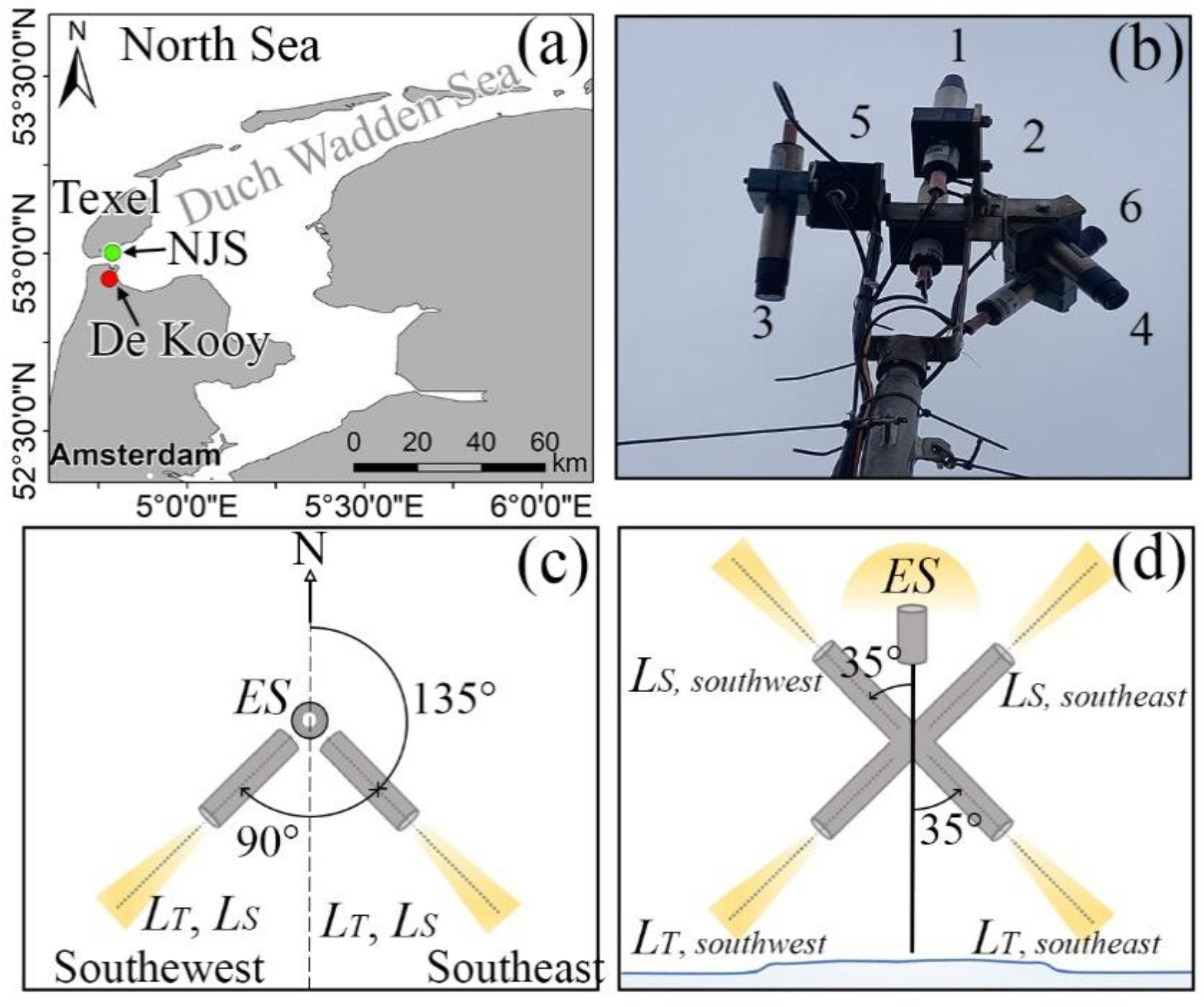
Figure 2.
Correlation between measured and estimated IOPs using the models in Table 1. Black-dashed lines are 1:1, red-dashed lines are linear regression, dotted-dashed lines are the confidence bounds of 95%. The comparative models are shown as hollow symbols for comparison.
Figure 2.
Correlation between measured and estimated IOPs using the models in Table 1. Black-dashed lines are 1:1, red-dashed lines are linear regression, dotted-dashed lines are the confidence bounds of 95%. The comparative models are shown as hollow symbols for comparison.
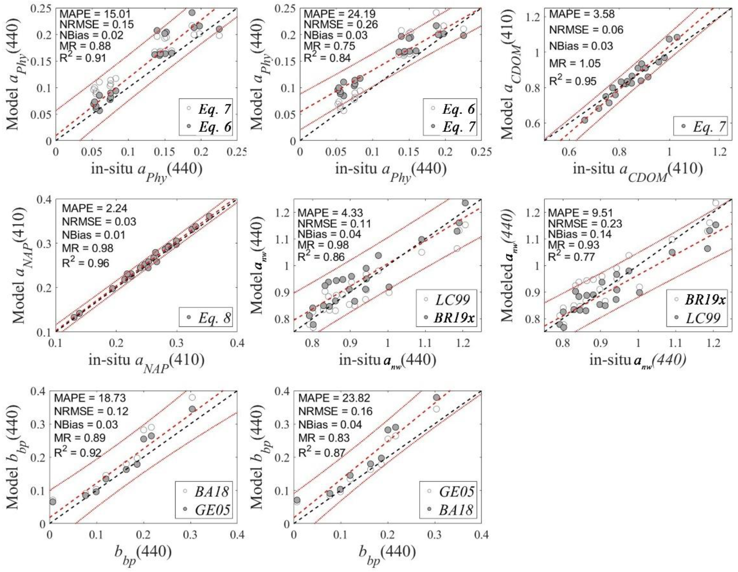
Figure 3.
The spectra of Rrs,ref(λ) and the average of modeled Rrs(λ) using various models outlined in Table 3 for different environmental conditions (Case I - Case VIII). The environmental conditions are illustrated in the text.
Figure 3.
The spectra of Rrs,ref(λ) and the average of modeled Rrs(λ) using various models outlined in Table 3 for different environmental conditions (Case I - Case VIII). The environmental conditions are illustrated in the text.
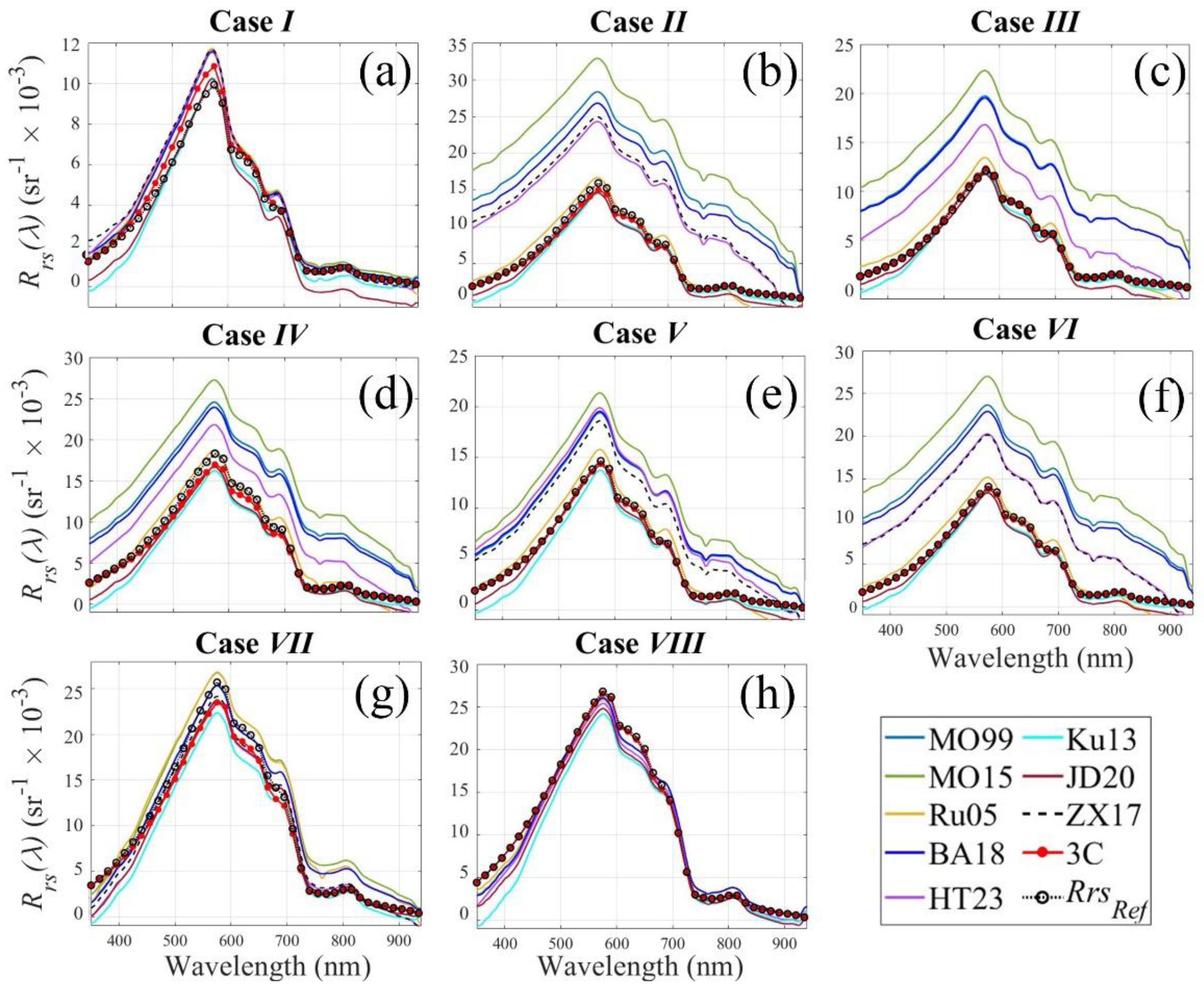
Figure 4.
The spectra of Rrs,ref(λ) and the average of modeled Rrs(λ) using various models outlined in Table 3 for different environmental conditions (Case I - Case VIII). The environmental conditions are illustrated in the text.
Figure 4.
The spectra of Rrs,ref(λ) and the average of modeled Rrs(λ) using various models outlined in Table 3 for different environmental conditions (Case I - Case VIII). The environmental conditions are illustrated in the text.
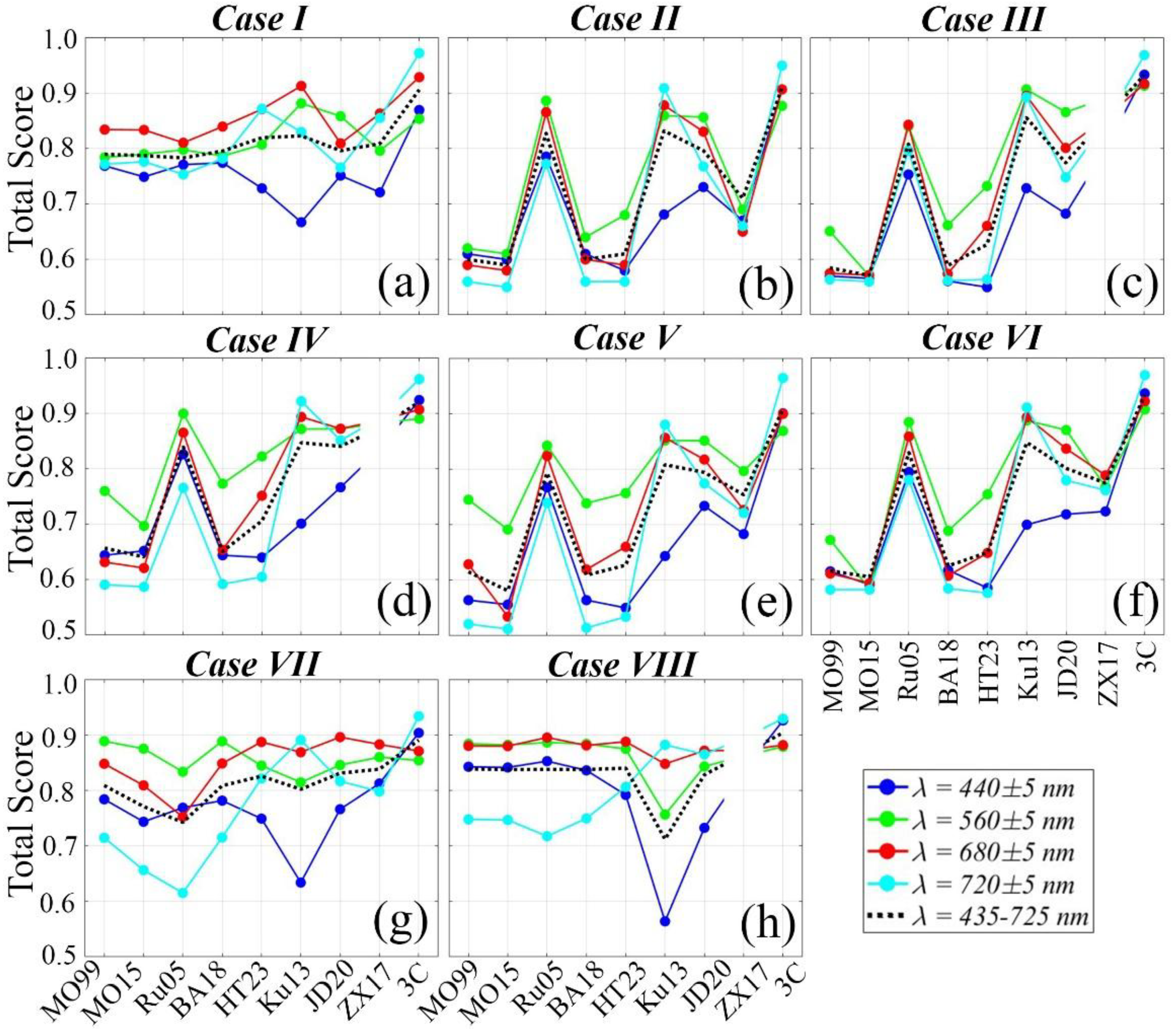
Figure 5.
a) Variations of ρ values obtained from models outlined in Table 3 for different environmental conditions (Case I - Case VIII). b) similar to (a), but for ΔL values. The environmental conditions are illustrated in section 4.2.
Figure 5.
a) Variations of ρ values obtained from models outlined in Table 3 for different environmental conditions (Case I - Case VIII). b) similar to (a), but for ΔL values. The environmental conditions are illustrated in section 4.2.
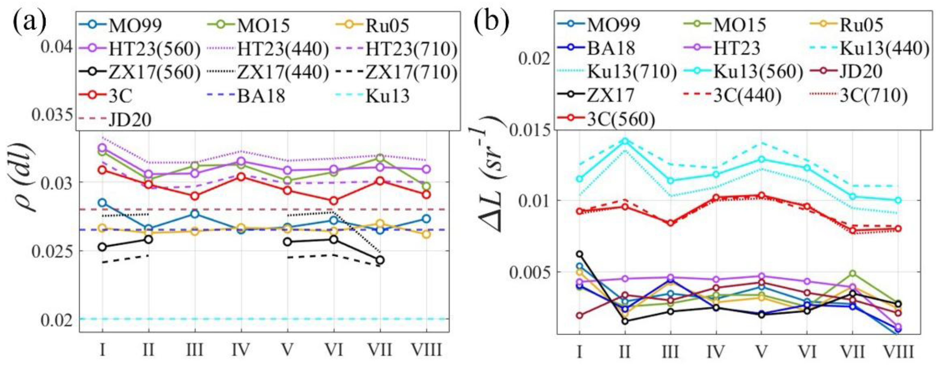
Figure 6.
Comparisons of QA scores of the total modeled Rrs(λ) spectra (N = 918) and Rrs,ref(λ) in various environmental conditions. The environmental conditions are illustrated in Section 4.2.
Figure 6.
Comparisons of QA scores of the total modeled Rrs(λ) spectra (N = 918) and Rrs,ref(λ) in various environmental conditions. The environmental conditions are illustrated in Section 4.2.
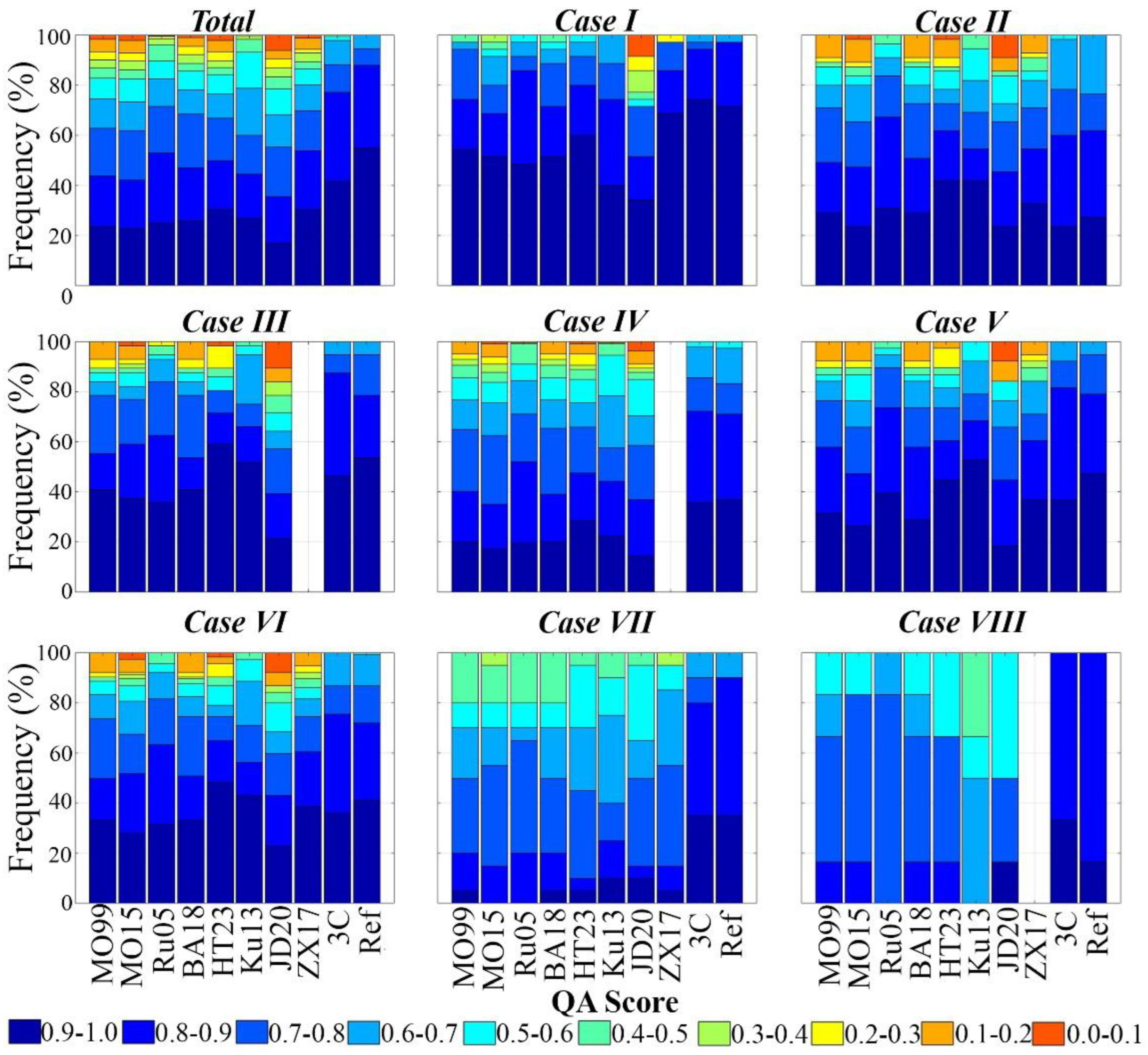
Figure 7.
Comparison of in-situ and estimated Chla using different models of Rrs. The dotted-red lines and dashed red lines show the statistical confidence level of 95%, and the linear trends, respectively. The dashed-black lines show the 1:1.
Figure 7.
Comparison of in-situ and estimated Chla using different models of Rrs. The dotted-red lines and dashed red lines show the statistical confidence level of 95%, and the linear trends, respectively. The dashed-black lines show the 1:1.
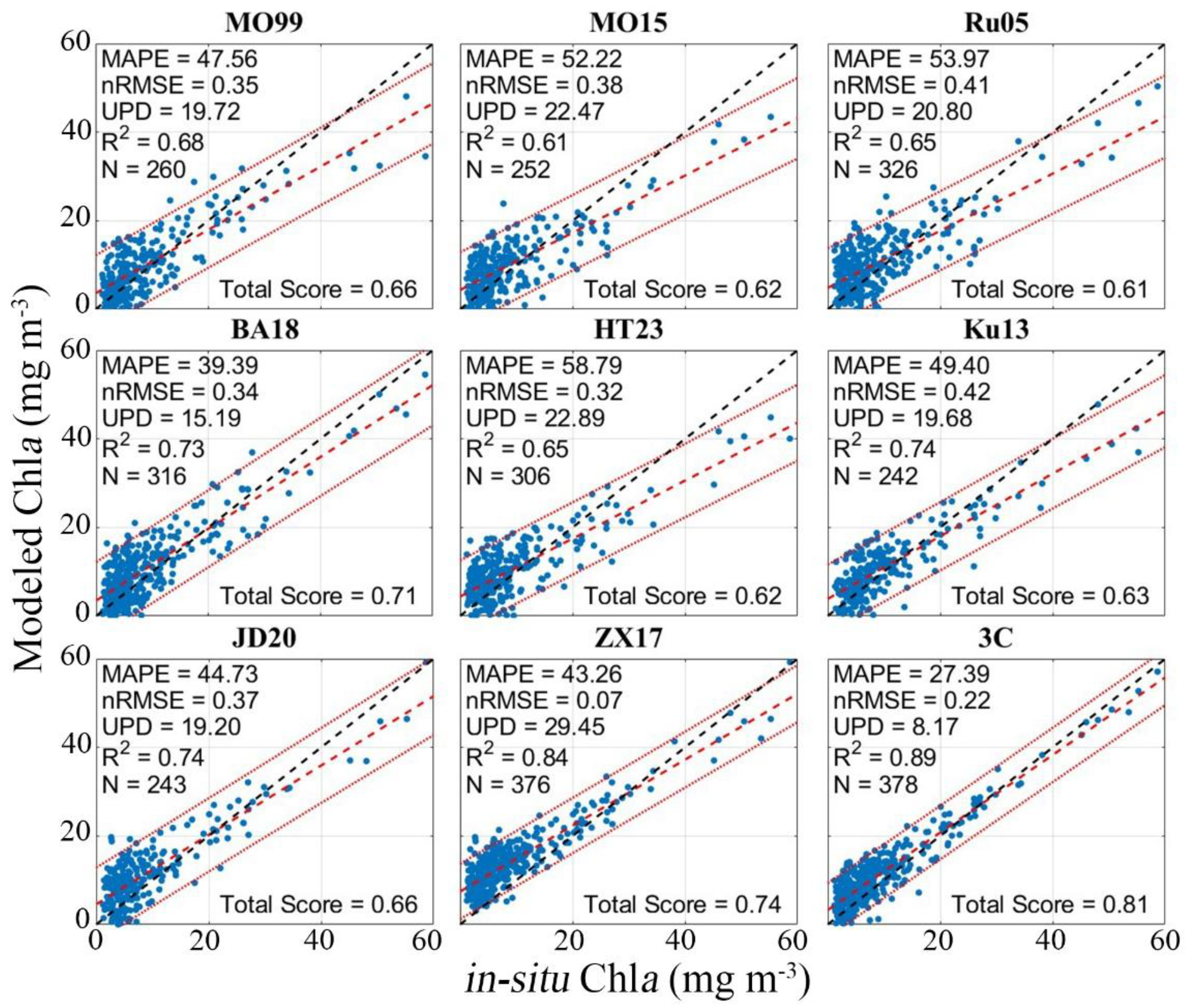
Figure 8.
Comparison of in-situ and estimated TSM using different models of Rrs. Symbols are similar to those in Figure 7.
Figure 8.
Comparison of in-situ and estimated TSM using different models of Rrs. Symbols are similar to those in Figure 7.
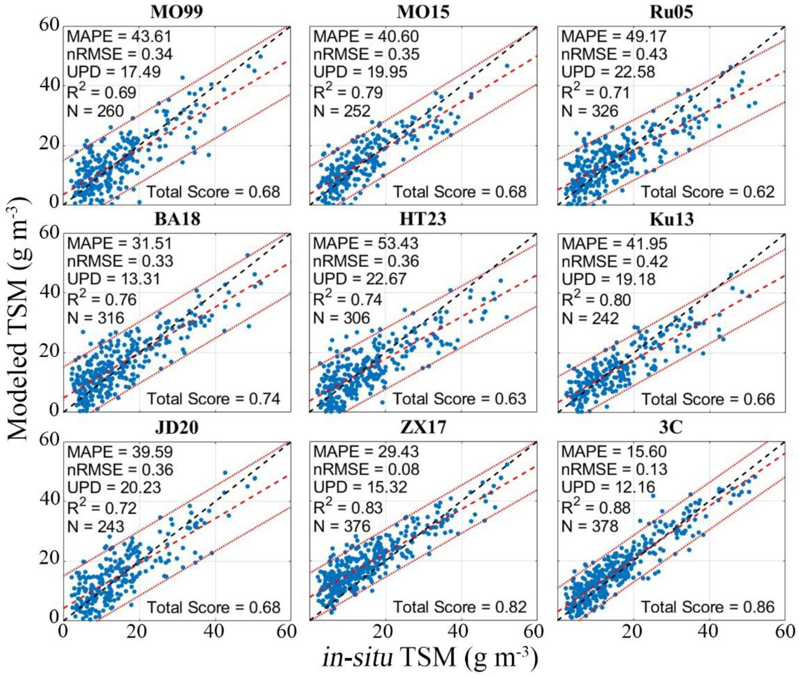

Table 1.
Methods of absorption and backscattering parametrization.
| Variable | Sym. | Parametrization | Ref. | Eq. |
|---|---|---|---|---|
| Chla-specific absorption | a*Chla | a* Chla(λ) = aPhy(λ)/[Chla] | [46] | (5) |
| Phy absorption | aPhy | aPhy(λ) = [Chla].a*Chla(λ) | [46] | (6) |
| Phy absorption a | aPhy |
aPhy(λ) = [a0(λ) + a1(λ) × ln(aPhy(λ1))] × aPhy(λ1) a aPhy(λ1) = 0.06 × [Chla]0.65 |
[47] | (7) |
| CDOM absorption | aCDOM | aCDOM(λ) = aCDOM(λ2) × exp[-SCDOM × (λ - λ2)] | [48] | (8) |
| NAP absorption | aNAP | aNAP(λ) = aNAP(λ2) × exp[-SNAP × (λ - λ2)] | [48] | (9) |
| Chla backscattering | bb,Chla | bb,Chla(λ) = {0.002 + 0.02 × [0.5 – 0.25 × log10[Chla] × (λ3/λ)]} × bb,Chla(λ3) , bb,Chla(λ3) = 0.416 × [Chl]0.766 | [34] | (10) |
| Chla backscattering b | bb,Chla | bb,Chla(λ) = [Chla] × b*b,Chla(λ3) × bNChla(λ) | [49] | (11) |
| NAP backscattering c | bb,NAP |
bb,NAP(λ)=bNAP(λ3)×(λ3/λ)γ - [1 – tanh(0.5 × γ2)] × aNAP(λ) bNAP(λ3) = b*SPM(λ3) × I × [SPM] |
[50] | (12) |
| NAP backscattering d | bb,NAP |
bb,NAP(λ) = [SPM] × b*b,SPM(λ) × bNNAP(λ) b*b,SPM(λ) = A × [SPM]B , bNNAP(λ) = a*Chla(λ3)/ a*Chla(λ) |
[49] | (13) |
Brackets indicate the concentrations of substances.λ1 = 443 nm, λ2 = 440 nm, λ3 = 550 nm a - a0(λ) and a1(λ) are the empirical wavelength dependents coefficients [51]. b - bNChla(λ) is the normalized backscattering of phytoplankton in coastal waters, b*b,Chla(λ3) = 0.001 m2 mg-1, from Gege (2005). c - I = 0.019 [52], γ = 0.6 [50]. d - A = 0.0006 m2 mg-1, B = -0.37 [53].
Table 2.
Statistical ranges of measured parameters in NJS for parametrization of bio-optical model.
| Parameter | Min | Max | Mean | Median | Std | N |
|---|---|---|---|---|---|---|
| Chla (mg m-3) | 0.44 | 51.48 | 9.080 | 6.31 | 2.56 | 648 |
| SPM (g m-3) | 2.20 | 82.40 | 16.06 | 12.75 | 5.98 | 648 |
| anw(675) (m-1) | 0.073 | 0.212 | 0.134 | 0.131 | 0.037 | 22 |
| anw(440) (m-1) | 0.792 | 1.206 | 0.934 | 0.901 | 0.128 | 22 |
| aPhy(675) (m-1) | 0.030 | 0.132 | 0.069 | 0.078 | 0.032 | 22 |
| aPhy(440) (m-1) | 0.052 | 0.224 | 0.119 | 0.138 | 0.055 | 22 |
| a*Chl(675) (m2 mg-1) | 0.014 | 0.021 | 0.017 | 0.017 | 0.002 | 22 |
| a*Chl(440) (m2 mg-1) | 0.022 | 0.036 | 0.028 | 0.029 | 0.004 | 22 |
| aNAP(440) (m-1) | 0.097 | 0.264 | 0.188 | 0.189 | 0.041 | 22 |
| a*NAP(440) (m2 mg-1) | 0.004 | 0.036 | 0.015 | 0.012 | 0.009 | 22 |
| SNAP (nm-1) | -0.011 | -0.009 | -0.01 | -0.01 | 0.001 | 22 |
| aCDOM(440) (m-1) | 0.441 | 0.906 | 0.621 | 0.599 | 0.103 | 22 |
| SCDOM (nm-1) | -0.013 | -0.008 | -0.011 | -0.011 | 0.001 | 22 |
| b*SPM(λ) (m2 mg-1) | 0.182 | 1.991 | 0.401 | 0.305 | 0.395 | 12 |
Table 3.
Methods of estimating ρ(θv,Δφ) and ΔL from above-water radiometric measurements (Equation (1)). The viewing geometry (θv,Δφ) and wavelength (λ) are omitted for simplicity.
Table 3.
Methods of estimating ρ(θv,Δφ) and ΔL from above-water radiometric measurements (Equation (1)). The viewing geometry (θv,Δφ) and wavelength (λ) are omitted for simplicity.
| Model | ρ(λ,θv, Δφ) | ΔL | Remarks | Ref. |
|---|---|---|---|---|
| MO99 | Lookup table of θv, Δφ, θs, and wind speed | min of Rrs(750-800) | ρ =0.028 in overcast and full ranges of wind speeds | [4] |
| MO15 | Similar to MB99 | improved values of ρ for sky polarization | [27] | |
| Ru05 a | ρ = 0.0256 in clear skies, ρ =0.0256 + 0.00039W + 0.000034W2 in cloudy |
Similarity spectrum normalization at 780 nm | ρ fits all simulations of 30≤θs≤70 with 1% err for W=5 and 3% for W=10 | [17] |
| BA18 | ρ = 0.0265 | min of Rrs(750-950) | Rrs(λ) optimized with a two-stream RT model | [28] |
| HT23 b | Lookup table of λ,θv,Δφ, θs, wind speed, and AOT. | min of Rrs(775-850) | RT computations used for AOT, polarization, and wind effects. Wavelength-dependent ρ. | [22] |
| Ku13 | ρ = 0.020 | Fitting a power function through the 350-380 nm and 890-900 nm regions. Wavelength-dependent ΔL | [21] | |
| JD20 | ρ = 0.028 | Relative height of the water-absorption-dip-induced-reflectance-peak-at-810 nm. It assumes ΔL is wavelength independent for variable cloud covers. | [20] | |
| ZX17 | Wavelength-dependent ρ. Lookup table of θv,Δφ, θs, wind speed, and AOT | min of Rrs(775-850) | Lookup table for: Wind speed:0,5,10,15 θs ≤ 60° AOT: 0,0.05,0.10, 0.20, 0.50 Clear Sky (cloud cover = 0) |
[2] |
| 3C | ρ and ΔL were estimated through optimization of LT(λ)/Ed(λ) modeling against measured LT(λ)/Ed(λ) using the fit parameters of IOPs and WCCs | It needs an overview of IOPs and WCCs, flexible for all environmental conditions. Wavelength-dependent ΔL | [16] | |
a- W = wind speed (m s-1). Identification of sky conditions was illustrated in Section 3.5.3. b- AOT = Aerosol Optical Thickness (Section 3.5.2).
Disclaimer/Publisher’s Note: The statements, opinions and data contained in all publications are solely those of the individual author(s) and contributor(s) and not of MDPI and/or the editor(s). MDPI and/or the editor(s) disclaim responsibility for any injury to people or property resulting from any ideas, methods, instructions or products referred to in the content. |
© 2025 by the authors. Licensee MDPI, Basel, Switzerland. This article is an open access article distributed under the terms and conditions of the Creative Commons Attribution (CC BY) license (http://creativecommons.org/licenses/by/4.0/).
Copyright: This open access article is published under a Creative Commons CC BY 4.0 license, which permit the free download, distribution, and reuse, provided that the author and preprint are cited in any reuse.


