A Comparative Study on the Acceptance of Autonomous Driving Technology by China and Europe: A Transnational Empirical Analysis Based on the Technology Acceptance Model

1. Introduction

Amid the global wave of vehicle electrification, China and Europe have both become mature leaders in the global transition toward intelligent mobility, serving as frontrunners in guiding the automotive industry from electrification to intelligent and automated transformation. Both Chinese and European markets possess large scale, well-established industrial ecosystems, and continuously promote technological innovation and broad application. New energy vehicles (NEVs) in the Chinese market have entered a stage of full-scale adoption, showing explosive growth. Year 2024 is a milestone year for China’s new energy vehicle market, with annual NEV production and sales exceeding 10 million units for the first time [1], and market penetration surpassing the historic threshold of 50% for the first time in July [2]. In terms of vehicle ownership, by the end of 2024, the total number of NEVs in China reached 31.4 million, accounting for 8.90% of the total number of vehicles; in 2024, 11.25 million NEVs were newly registered, accounting for 41.83% of all newly registered vehicles [3], indicating that NEVs are gradually becoming mainstream in the Chinese market. The European NEV market has also continued to grow in recent years, with the number of NEV registrations in 2023 increasing by nearly 20% compared to 2022 [4]. In terms of market competition, the best-selling electric vehicle brands in Europe are mostly European and American brands [5]. At the same time, the European Union has set a goal of large-scale NEV deployment by 2030 and plans to ban the sale of new gasoline cars and small commercial vehicles that cause carbon emissions starting from 2035 [6,7]. Driven by both policy support and normative consumer acceptance, China and Europe are jointly leading the global electrification transformation of the automotive industry. Against the backdrop of a steadily strengthening NEV industry, accelerating the development of autonomous driving technology has become an inevitable choice for both China and Europe. The mature electrification platforms provide an ideal electrical architecture and data foundation for autonomous driving, and autonomous driving technology has become a core competitive domain in the development of NEVs and a central track in technological competition [8]. Faced with global technological competition and technological revolution, only by achieving breakthroughs in the field of autonomous driving can China and Europe consolidate their leadership in the NEV sector and define a new paradigm in future mobility technology.

The development and advancement of autonomous driving technology not only represent a revolutionary breakthrough in artificial intelligence within the field of transportation, but also hold the potential to profoundly reshape the future structure of human society and the global economy. However, as autonomous driving technology gradually moves from the laboratory to real using roads, the controversies and risks it brings are becoming increasingly prominent. On March 29, 2025, a Xiaomi electric vehicle SU7 was involved in a fatal accident that drew national attention, which occurred on the Zongyang Expressway in Tongling, Anhui Province, China. The vehicle was driving at a high speed of 116 km/h during nighttime with NOA assisted driving system activated and this system failed to recognise a stationary obstacle ahead, resulting in a violent collision and subsequent fire that caused the deaths of all three occupants. It is worth noting that the NOA assisted driving system of the vehicle can be regarded as a Level 2 (L2) assisted autonomous driving system. After the incident, Xiaomi released the relevant vehicle data, which showed that there was only less than two seconds of manual takeover time before the collision. Although the system issued a warning after visual recognition, it failed to activate the Automatic Emergency Braking (AEB) function in time, ultimately leading to the tragedy [9,10]. At present, autonomous driving technology is still in a stage of technical immaturity, especially in key capabilities such as visual recognition, multi-source perception, and emergency response. This technology is still struggling to handle all complex road scenarios. The core problems exposed by the Xiaomi SU7 accident was the system’s failure to recognise static obstacles and the AEB system’s failure to intervene in time [10]. These problems essentially reflect the limitations of current assisted driving systems in coping with extreme situations. This incident quickly fermented in the sphere of public opinion, triggering widespread safety concerns and renewed debate about intelligent and autonomous driving technologies. Public concern has mainly focused on three aspects: first, whether the system’s ability to identify obstacles and avoid them is sufficiently safe and reliable, second, whether emergency rescue mechanisms during autonomous driving are reasonable and effective, and third, whether car companies are over-marketing these technologies and leading users to trust the systems beyond their actual capability, despite the technology’s immaturity [11]. These doubts clearly demonstrate that before autonomous driving becomes part of everyday public life, it still faces severe challenges in terms of social acceptance and public awareness.

Therefore, when discussing the development of autonomous driving technology, it is essential to attach great importance to public acceptance, as public acceptance determines the social foundation of the technology. In the absence of a thorough understanding of autonomous driving technology, ordinary consumers often find themselves in a gray area between trust and fear. Following major accidents, consumer and market attitudes toward autonomous driving technology experience sharp fluctuations, with the public questioning the safety, maturity, and practical application of the technology, especially how to ensure that the system can seamlessly and safely replace human drivers in complex road environments. Through the Xiaomi SU7 accident, it becomes clear that the promotion of technology is not merely about the success or failure of the product itself, but also deeply involves public acceptance of the new technology, which affects the ultimate implementation and effectiveness of the technology [12]. Acceptance determines whether consumers are willing to try and use autonomous driving systems in the long term. If a technology fails to achieve widespread social acceptance, or if consumers are unable to rationally accept its limitations, the technology may face stagnation or even backlash. Academic research, industrial development, and policy guidance must all simultaneously pay attention to this crucial dimension during the process of technological promotion. In the context of a high-risk technology such as autonomous driving, ensuring transparency, safety, and comprehensive public education is vital for the healthy implementation of the technology. Only when social acceptance and rapid technological advancement are effectively balanced can autonomous driving technology achieve widespread adoption on a global scale and deliver its intended social benefits [13]. Consequently, focusing on the acceptance of autonomous driving technology is not only an embodiment of technological ethics but also the very foundation for the implementation of the autonomous driving industry.

It is evident that the large-scale production and application of autonomous driving, and its eventual creation of economic and social value, not only depend on technological innovation and maturity but are also profoundly constrained by the level of acceptance across different markets. The attitudes of markets and consumers toward autonomous driving will largely influence the actual application of driverless technology [13]. China and Europe, as two of the world’s most significant automotive markets, both demonstrate a high level of attention to autonomous driving technology and are at the forefront globally in terms of technological advancement [4]. However, there are notable differences between China and Europe in policy orientation, infrastructure, social culture, and consumer psychology. Theses differences inevitably lead to differing perceptions, attitudes, and expectations toward driverless technology in the two markets. As the two largest new energy vehicle markets in the world, China and Europe differ in consumer acceptance and expectations of autonomous driving. This has irreplaceable strategic value for developing localized technology strategies, helping policymakers improve regulatory frameworks, and guiding industry players in precise resource allocation. It is also an important benchmark for determining the future direction of the automotive industry and holds great significance for both China and Europe.

2. Why Should We Study the Acceptance of Autonomous Driving Technology Between China and Europe?

2.1. Chinese Consumers’ Acceptance of Autonomous Driving Technology

From the perspective of consumer acceptance, Chinese consumers show significant differences with European consumers. First, compared with consumers in high-income countries, Chinese consumers generally demonstrate a higher level of acceptance toward autonomous driving technology. According to the report by Cui Liyong et al., Chinese consumers have a high level of acceptance of autonomous driving technology in the world [14]. Data from J.D. Power in 2021 show that 10% of Chinese consumers express complete trust in autonomous driving technology, 68% say they might trust it, and only 4% express complete distrust. This is largely due to the widespread support for Advanced Driver Assistance Systems (ADAS) in existing vehicle models in Chinese market [15]. This conclusion is further supported by other surveys, which indicate that Chinese consumers hold a positive attitude toward L1–L2 level assisted driving. Such trust stems from the rapid adoption of L2-level assisted driving, with L2 models accounting for 42.4% of new car sales in China during the first half of 2023, allowing consumers to build familiarity with the technology through everyday use [16,17].

However, Chinese consumers seem to remain cautious about both daily use and the adoption of fully autonomous driving. For example, data from J.D. Power show that only 9% of Chinese consumers accept scenarios where fully autonomous driving technologies, such as Robotaxi, completely replace human driving [15]. According to Business Sweden, more than half of Chinese consumers take a wait-and-see approach rather than fully embracing the technology [16]. A 2019 study by Wei Xiaoxiao et al. suggests that authorities should strengthen promotion, improve functions and services, and enhance user-friendliness to raise acceptance [18]. This indicates that in the civilian sector, public awareness of autonomous driving is still limited, and actual acceptance may be less optimistic than earlier described. Tang Li et al. reached a similar conclusion: reported high acceptance often comes from respondents under highly hypothetical scenarios, most of whom have little real experience with autonomous vehicles [19]. This may cause gaps between survey predictions and market reality. Qin Hua’s research on Tesla owners in Beijing offers further evidence. It shows that safety concerns reach 31.8% when buying cars with autonomous driving systems. Even after learning to use the technology, 70% of owners activate it in only 30% of their driving [20]. Wan Dan et al. found that in the civilian sector, consumers have doubts about safety and data privacy, reflecting low trust in reliability. In the military sector, however, acceptance is higher due to mandatory use and government endorsement [21]. Wang Maoan’s study also suggests that manufacturers should highlight safety of autonomous vehicles to ease consumer concerns [12]. This also means that not all Chinese consumers trust autonomous driving technologies so much. Overall, Chinese consumers need a more comprehensive understanding of autonomous driving to raise acceptance in civilian use. While they show high awareness of the concept and future potential, they also express skepticism and distrust in real-world applications.

In Chinese society, continuous government policy support and the steady expansion of application scenarios are key driving forces in improving public acceptance of new technologies. Under policy guidance, Chinese consumers show strong recognition of domestic technological breakthroughs. The Intelligent Vehicle Innovation and Development Strategy sets clear phased goals for autonomous driving, such as the production target for autonomous vehicles in 2025 [22]. Standardization and regulation promoted by policy can reduce consumer concerns about autonomous driving and increase psychological acceptance of the technology. While boosting consumer confidence, policy guidance also accelerates the deployment of key infrastructure such as vehicle-road collaboration systems, reducing environmental uncertainties during implementation. Building infrastructure ahead of time paves the way for technology adoption, improving the market’s ability to adapt and shortening the integration period between new technology and the market, which in turn increases acceptance. In addition, policy support makes it easier for companies in the autonomous driving sector to obtain government subsidies, lowering costs for both production and consumers. This reduces the financial barrier for adopting the technology and further improves public acceptance. Successful practices in specific commercial scenarios also build tangible trust among the public and the market. According to Business Sweden, autonomous driving solutions for mines and ports—where labor costs, accident rates, and operational difficulty are high—have already led to large-scale commercial adoption in those sectors. For example, in the Guoneng Baorixile open-pit coal mine project, autonomous mining trucks operated efficiently despite extreme cold and hazardous conditions, significantly reducing labor costs, accident rates, and operational challenges [15]. This project not only promoted the commercialization of autonomous driving in mining scenarios but also boosted market confidence and provided a model for similar environments, greatly improving acceptance of the technology in Chinese market. High-success-rate and highly visible case studies like this significantly enhance trust in technical performance, which strengthens the willingness to adopt on a psychological level. In conclusion, policy guidance and infrastructure deployment are major reasons for Chinese consumers’ acceptance of new technology, while successful real-world applications further stimulate market confidence in specific scenarios [23].

2.2. European Consumers’ Acceptance of Autonomous Driving Technology

Compared with consumers from China, European consumers, while open to purchasing and using new energy vehicles, are clearly more conservative and cautious about autonomous driving. Schoettle’s research shows that although respondents in both high-income and low-income countries are concerned about the safety of autonomous driving, acceptance levels are notably lower in high-income countries. For example, respondents from the United Kingdom show lower acceptance than those from China and India [24]. Research by Nordhoff et al. also finds that respondents from low-income countries have higher acceptance of autonomous driving technology [25]. According to Cui Liyong et al., acceptance in Western countries is generally lower than in the Asia-Pacific region [14]. Anania et al. (2018) also report that respondents in high-income countries hold more negative attitudes toward autonomous driving [26]. Hudson et al. further point out that most respondents from EU countries have a negative view of the technology [27]. A study by dos Santos et al. on the situation in Europe shows that 55.6% of respondents have a negative attitude toward autonomous vehicles. EU citizens feel uncomfortable both purchasing and riding in autonomous vehicles, question their safety and reliability, and many also express concerns about potential threats to personal privacy [28]. Overall, European consumers show relatively low acceptance of applying autonomous driving technology in everyday life.

It is worth noting that, according to relevant EU reports and studies on the state of autonomous driving in Europe, one possible reason for European consumers’ low acceptance is that the technology is still at the L3, or lower conditional automation, stage. Consumers have limited real-life experience with fully autonomous driving (L4+), which makes it difficult to increase acceptance [28,29,30,31]. This is reflected in a survey by Salonen et al., in which Finnish respondents who had ridden autonomous buses expressed higher recognition of their safety and showed more tolerance toward accidents involving them compared to traditional buses [32]. This suggests that the public and consumers may need more direct experience and understanding of fully autonomous driving before acceptance can improve. It can be seen that even though the EU continues to promote policies for decarbonisation and smart mobility, public concerns about autonomous driving remain. These concerns stem partly from distrust of the current technology and partly from worries about potential ethical and privacy issues. In addition, inadequate infrastructure, as well as the high purchase and usage costs of autonomous vehicles, further reduce European consumers’ acceptance [33].

Another key prerequisite for European consumers to accept autonomous driving technology is the standardization of its ethical norms and the clear definition of responsibility. For example, Hajjafari’s research shows that respondents strongly demand a legal framework for autonomous driving, and that government regulation and policy support are important factors in improving acceptance [34]. Respondents also tend to assign responsibility to manufacturers when accidents occur, reflecting the importance they place on accountability in autonomous driving incidents [34]. In addition, Adnan et al. found that a crucial factor influencing acceptance is how responsibility is assigned among vehicles, pedestrians, passengers, and manufacturers [35]. The 2018 European Parliament study report emphasised that consumers regard a clear framework for accident liability and robust data protection laws as prerequisites for the technology’s deployment [36]. When facing autonomous driving technology, European consumers are concerned more about legal standardization and responses to ethical and legal disputes than about rapid application and implementation. Zhu Jinwen’s research also shows that Chinese intelligent driving new energy vehicles entering overseas markets must comply with Europe’s strict data governance regulations, and that 53% of respondents express concerns about data security. Chinese automakers, therefore, need to adopt strategies aligned with European consumer habits [37]. This demonstrates that both at the institutional level and in terms of consumer psychology, acceptance in the local market is built on a foundation of strong legal and ethical safeguards.

In addition to the need for legal and ethical standardization, the European market also emphasizes the role of autonomous driving in delivering social benefits. Unlike the Chinese market, which focuses on the “tool attributes” and “production efficiency” of the technology, the European market tends to integrate autonomous driving with broader goals such as environmental sustainability and safety governance. For instance, the EU’s Sustainable and Smart Mobility Strategy identifies autonomous driving as a key means of building an efficient, zero-emission transport system. Policy planning for the future of European transport has stimulated market vitality for autonomous driving and significantly increased acceptance [38]. Net-Zero Industry Act: Accelerating the transition to climate neutrality also explicitly requires autonomous driving technology to contribute to carbon neutrality goals, binding it at the policy level to green and environmental objectives and highlighting its role in reducing emissions and supporting carbon neutrality [39].According to dos Santos’s research, respondents value autonomous driving for its ability to reduce accident rates, ease traffic congestion, and cut carbon emissions [28]. This approach to technology acceptance, which places greater weight on social value, underscores the European market’s high sensitivity to both ethical legitimacy and positive societal impacts.

2.3. The Necessity of Further Paying Attention to the Acceptance of Autonomous Driving Technology

It can thus be seen that although the development paths of autonomous driving technology in China and Europe each have their own characteristics, both are highly dependent on the steady improvement of public acceptance. In China, policy guidance and infrastructure development will remain the core drivers for the technology’s implementation, while the continued expansion of commercial application scenarios will further strengthen public recognition of the technology’s usability. However, an important challenge remains in ensuring data security and clarifying legal responsibility while preventing fluctuations in technological trust caused by isolated incidents. In contrast, Europe places greater emphasis on building institutional norms and ethical frameworks in advance. The application of the technology must be fully supported by legal guarantees, privacy protection, and social benefits, and the improvement of acceptance will mainly rely on the accumulation of real-world experience and the steady advancement driven by policy. The acceptance paths in the two regions reflect differences in institutional logic and the social cognitive foundations, which in turn determine the focus areas and pace of future development of autonomous driving technology.

Based on the above research, although studies on public acceptance of autonomous driving technology in China and Europe have achieved preliminary results, they still face problems such as insufficient timeliness of data, concentrated research perspectives, and a relatively simple theoretical structure. Most existing empirical data are concentrated between 2018 and 2023, making it difficult to fully reflect the latest changes in the speed of technological deployment, fluctuations in public opinion, and shifts in public attitudes during the current period of rapid development in autonomous driving technology. Around 2025, with the large-scale commercial deployment of L2–L3 and even more advanced assisted autonomous driving systems, as well as the normalization of increasingly diverse Robotaxi operations, autonomous driving systems are evolving from assistance functions toward higher-level intelligent autonomous decision-making. Their frequency of application in real traffic environments continues to rise, along with increases in system complexity and social sensitivity [40]. During this process, public acceptance of autonomous driving is influenced by more diverse factors, no longer limited to the advanced nature of the technology itself, but extending to broader social dimensions such as legal liability, ethical boundaries, privacy protection, and accident handling. Meanwhile, the frequent occurrence of a new wave of typical incidents has caused fluctuations in the foundation of public trust, further reinforcing the academic and industrial focus on social acceptance as a non-technical variable.

Against this background, centring on more reality-oriented questions, updating the latest data, and integrating reliable research models to reassess the social acceptance of autonomous driving technology not only responds to public concerns but also serves as essential theoretical preparation for effective technological implementation. This study is based on that starting point, aiming to empirically capture the changing trajectory of public psychological structures in China and Europe, and to clarify the differences in the paths of technological acceptance between the two regions. Behind these differences lie consumer judgments of the technology’s functionality and safety, as well as the influence of institutional structures, risk perception, and cultural trust systems. Therefore, carrying out an acceptance study that combines regional comparability with structural mechanisms not only has strong practical relevance but also holds significant potential for theoretical contribution.

3. Model Building

3.1. Model Selection and Parameters Setting

In terms of theoretical and methodological choice, the Technology Acceptance Model (TAM), widely recognised in the international academic community as a mainstream framework for studying technology–user behaviour, offers strong adaptability and scalability. The model is simple in structure, logically clear, and highly adaptable in terms of variables, making it widely used to study how new technologies are perceived, evaluated, and adopted by the public. Since Davis introduced it in 1989, TAM has been extensively applied in fields such as information systems, mobile internet, e-commerce, artificial intelligence, and shared mobility. Its core logic centres on two fundamental questions: whether users perceive the technology as useful and whether they find it easy to use [41]. These two dimensions form the key starting point for shaping user attitudes and, through a behavioural intention path model, further predict actual usage behaviour. By analysing the two core constructs—Perceived Usefulness (PU) and Perceived Ease of Use (PEOU)—TAM provides researchers with a concise, effective, and easy-to-operate theoretical tool for predicting and explaining user acceptance of emerging technologies. This is especially relevant in contexts involving high uncertainty and strong risk perception, where TAM proves highly applicable in explaining the psychological process of trust building–risk assessment–acceptance decision.

In recent years, with the continuous expansion of TAM, many studies have incorporated variables such as risk perception, institutional trust, ethical judgment, and social influence. These extensions, while retaining the original model’s simplicity, enable better adaptation to complex real-world contexts, forming a flexible application paradigm of basic model plus extended variables. In the field of transportation, multiple empirical studies have confirmed TAM’s high level of fit and explanatory power in interpreting user acceptance of emerging technologies such as car sharing and autonomous driving [18,21,42,43,44]. Its advantages lie not only in the clarity of relationships between variables and the rationality of its path design but also in its ability to integrate social variables from different cultural and institutional contexts, thereby producing a comparable and transferable analytical framework. The primary reason for selecting TAM is its simplicity and efficiency. Compared with other theoretical models, TAM can effectively explain the main drivers of technology acceptance through just two dimensions: Perceived Usefulness (PU) and Perceived Ease of Use (PEOU). Perceived Usefulness focuses on an individual’s belief that a technology enhances efficiency or reduces workload, while Perceived Ease of Use evaluates whether the technology is easy to operate [45,46]. In the context of autonomous driving, Perceived Usefulness relates to public recognition of the technology’s ability to improve travel efficiency and reduce traffic accidents, while Perceived Ease of Use concerns the system’s operational simplicity and user-friendliness. These two dimensions play a decisive role in public acceptance. In studying acceptance of this emerging technology, TAM’s clear and straightforward framework allows us to identify the core factors influencing technology adoption without introducing an excessive number of complex variables and measurement items, thereby simplifying the analysis process.

Compared with other models such as the Theory of Planned Behavior (TPB) and the Unified Theory of Acceptance and Use of Technology (UTAUT), which can offer a more comprehensive explanation, these frameworks often include multiple complex variables and are better suited for large-scale, long-term data collection and research [47,48]. At the early stage of studying technology acceptance, using such models may result in excessive complexity. Therefore, the simplicity of TAM makes it the most appropriate choice for current research on the acceptance of autonomous driving technology.

Another major advantage of TAM is its strong cross-cultural applicability. Although technology acceptance can be influenced by differences in regional and cultural contexts, TAM’s core constructs—Perceived Usefulness (PU) and Perceived Ease of Use (PEOU)—are highly adaptable and can effectively support acceptance studies across different cultural and social settings. Specifically, in this study, China and Europe differ significantly in cultural traditions, social structures, and policy contexts, yet TAM can provide a unified analytical framework to reveal similarities and differences in how the public in these two regions accepts autonomous driving technology [18,21,42,44]. By adding appropriate extended variables to the TAM framework, it is possible to further examine how cultural and social factors influence public acceptance of autonomous driving. This flexibility is another key advantage of TAM, allowing researchers to adjust the model according to specific research needs and to account for local cultural differences and potential barriers to technology adoption.

Therefore, due to its simplicity, effectiveness, and strong cross-cultural adaptability, TAM is the optimal choice for this study. Applying TAM to a comparative analysis of public acceptance of autonomous driving in China and Europe not only revalidates the model’s cross-cultural effectiveness but also extends its theoretical scope within the context of intelligent transportation technologies. Given the marked differences in political systems, legal frameworks, cultural mindsets, and media environments between China and Europe, the mechanisms through which the public forms attitudes toward autonomous driving may vary structurally: for example, Chinese citizens may be more influenced by policy guidance, industry application scenarios, and positive incentives from infrastructure deployment, whereas European citizens may place greater emphasis on ethical legitimacy, privacy protection, and clear institutional accountability. Conducting variable comparisons and path analyses within a unified model framework enables the identification of significant perceptual differences between the two regions and provides insight into the institutional roots of these differences. This study, through its updated data, focused research questions, and deliberate model choice, responds to the urgent needs and contemporary challenges of autonomous driving research. By integrating TAM with a China–Europe comparative perspective, it seeks not only to offer an analytical approach capable of explaining cross-cultural differences in public acceptance but also to provide theoretical support and policy references for technology promotion strategies, public risk communication mechanisms, and institutional design.

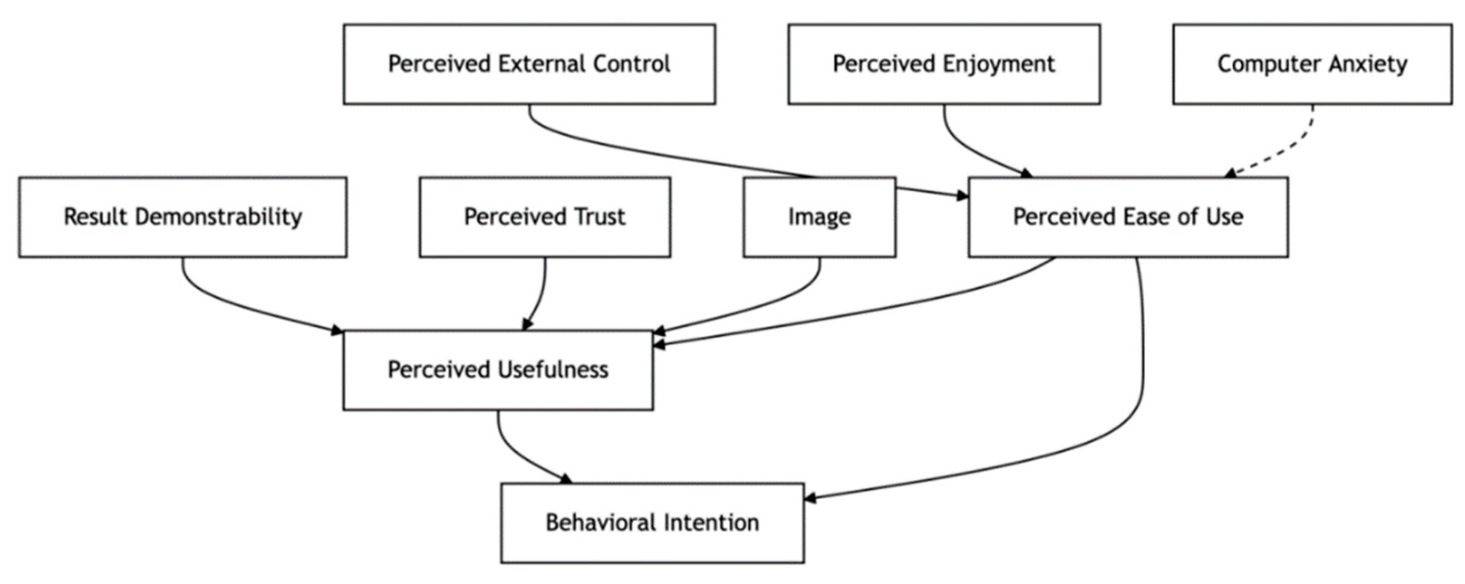
Against this background, this study designs variables within the PU (Perceived Usefulness) dimension focusing on three types of benefits: Result Demonstrability (RD), Image (IMG), and Perceived Trust (PT). First, the RD variable primarily addresses users’ perceived utility of autonomous driving technology in improving travel efficiency, reducing traffic accidents, and enhancing environmental quality. Previous studies have indicated that autonomous driving systems can improve traffic efficiency and save travel time through intelligent route planning and vehicle-to-everything (V2X) functions [49]. In addition, autonomous driving systems can effectively reduce empty trips and optimize route selection through intelligent scheduling, thereby significantly contributing to energy conservation, emission reduction, and the realization of green travel goals. Consequently, environmental factors have become an important dimension influencing perceived usefulness [38,50]. Second, the IMG variable reflects users’ perception of the symbolic meaning of autonomous driving technology as a marker of technological progress. Related studies have shown that some users view the adoption of autonomous driving as a way of keeping up with technology and participating in the future of mobility [51]. This sense of status recognition, when incorporated into an extended TAM model, serves as an important socio-psychological mechanism affecting perceived usefulness and behavioral intention. Third, the PT variable emphasizes users’ concerns about technological legitimacy, data privacy protection, and ethical controllability—dimensions that have become increasingly salient in countries like China, where autonomous driving technology is being rapidly deployed. Previous research has shown that when evaluating whether a technology is worth adopting, users not only consider whether it is “useful” but also whether it is compliant, controllable, and respectful of privacy. This makes ethical and legal norms an essential component in constructing perceived usefulness [24,52].

In the PEOU (Perceived Ease of Use) dimension, this study constructs a variable system from three perspectives: Perceived External Control (PEC), Perceived Enjoyment (ENJ), and Computer Anxiety (CANX). First, PEC emphasises users’ perceived ease of use within their operational environment, such as whether there is adequate policy and regulatory support, well-developed road infrastructure, and clear, accessible user guidance. Empirical studies have also confirmed that this factor is highly applicable in research on autonomous driving acceptance [34,53]. Second, ENJ focuses on users’ sensory and emotional experiences during use, such as whether autonomous driving offers greater comfort, entertainment facilities, or the ability to free one’s hands and experience enjoyment. Such motivations are receiving growing attention in the transportation sector [54,55]. Third, the CANX variable addresses users’ trust in the operational stability and emergency handling capabilities of autonomous driving systems, particularly concerns about system failures or being forced to take control in uncertain situations. Xu has pointed out that the safer autonomous vehicles are, the stronger users’ overall willingness to accept them [56], and Dong’s research also indicates that when vehicles operate under higher levels of regulatory oversight, respondents’ willingness to accept autonomous driving increases [53].

In the Behavioural Intention (BI) dimension, this study designs three categories of measurement items, focusing respectively on users’ usage tendency, choice priority, and willingness to engage in word-of-mouth promotion. The BI measurement is not only used to determine whether users are willing to incorporate autonomous driving into their daily travel routines, but also whether, when choosing among different transportation options, they would prioritise autonomous driving solutions, and whether they are willing to actively recommend this technology to others. In an empirical study comparing the acceptance of autonomous driving between Chinese military personnel and civilians, Wan and Peng found a highly significant positive relationship between perceived usefulness (PU) and behavioral intention (BI) [21]. Perceived ease of use (PEOU), on the other hand, tends to influence BI indirectly through PU, while users’ recommendation willingness often reflects their overall recognition of the technology, making it a strong predictor and a key factor in social diffusion [21].

In summary, the measurement variables in this study are constructed strictly in accordance with the logical pathways of the TAM model, while incorporating social value, ethical perception, and emotional variables unique to the autonomous driving context. This ensures that the variable system not only maintains the theoretical consistency of the model but also fully addresses the complex needs arising in practical application scenarios. By systematically measuring the three major dimensions—PU, PEOU, and BI—this study can comprehensively reveal Chinese consumers’ acceptance logic toward autonomous driving technology, providing both theoretical support and practical insights for relevant policy-making and technology promotion.

3.2. Build TAM Model Based on the Above Parameters

Figure 1. Technology Acceptance Model Framework.

Figure 1. Technology Acceptance Model Framework.

3.3. Accordingly, the Following Hypotheses are Proposed

Hypothesis 1: 

If autonomous driving technology can improve my travel efficiency and convenience, I will be more willing to choose to use autonomous driving technology.

Hypothesis 2: 

If autonomous driving technology can reduce the occurrence of traffic accidents, I will be more willing to accept this technology.

Hypothesis 3: 

If autonomous driving technology can reduce carbon emissions and improve the environment, I will be more willing to accept this technology.

Hypothesis 4: 

If adopting and using autonomous driving technology allows me to feel aligned with cutting-edge technology, I will be more willing to choose it.

Hypothesis 5: 

If the use of autonomous driving technology reflects my recognition of technological innovation, I will be willing to accept it.

Hypothesis 6: 

If using autonomous driving technology symbolises my support for technological development and social progress, I will be more willing to try and accept this technology.

Hypothesis 7: 

If autonomous driving technology is fully regulated in terms of legal and ethical safeguards, I will be more willing to trust the safety of this technology.

Hypothesis 8: 

If autonomous driving technology can handle ethical dilemmas in accordance with widely accepted ethical frameworks, I will find it easier to accept the use of autonomous driving technology.

Hypothesis 9: 

If autonomous driving technology fully protects users’ privacy rights and takes measures to ensure data security, I will find it easier to accept the technology.

Hypothesis 10: 

If the government provides sufficient policy support and introduces corresponding laws and regulations, I will consider it easier to use autonomous driving technology.

Hypothesis 11: 

If companies and manufacturers related to autonomous driving technology provide detailed and reliable usage guidance and technical support, I will find it easier to get started with using autonomous driving technology.

Hypothesis 12: 

If local infrastructure—such as intelligent traffic signals and dedicated lanes—has been prepared for the application of autonomous driving technology, I will find it easier to accept using autonomous driving for travel.

Hypothesis 13: 

If I can gain more enjoyment from using autonomous driving compared to traditional driving, I will be more willing to accept and use autonomous driving systems.

Hypothesis 14: 

If using autonomous driving technology can provide higher comfort compared to traditional transportation modes, I will be more inclined to choose this technology.

Hypothesis 15: 

If autonomous driving technology can offer more diverse in-car entertainment options, such as in-car cinemas or gaming consoles, I will be willing to try it.

Hypothesis 16: 

If I feel nervous and anxious while using autonomous driving technology due to the need to constantly pay attention to whether I need to take over the vehicle, I may avoid using the technology.

Hypothesis 17: 

If the autonomous driving system cannot respond promptly to emergencies when it malfunctions, I will develop doubts and resistance toward autonomous driving technology.

Hypothesis 18: 

If autonomous driving technology proves to be highly effective in improving travel efficiency, reducing accidents, and enhancing the environment, I will consider it a technology worth accepting and using.

Hypothesis 19: 

If the autonomous driving system is not only technologically advanced but also equipped with clear legal liability allocation and ethical standards, I will regard it as a trustworthy mode of transportation.

Hypothesis 20: 

If autonomous driving technology in practical application can both reflect the development of science and technology and improve travel experiences, I will be more inclined to view it as a technology worthy of large-scale adoption.

Hypothesis 21: 

If I can obtain clear and understandable operational guidance and scenario demonstrations before using autonomous driving technology, I will find it easier to understand and accept how to use the technology.

Hypothesis 22: 

If the autonomous driving system can operate autonomously, steadily, and safely under normal driving conditions without causing me to feel continuously tense or overly alert, I will consider it suitable for daily use.

Hypothesis 23: 

If the deployment of autonomous driving technology receives policy support, is accompanied by cooperative infrastructure, and is supported by public education, I will find it easier to accept the usage scenarios of this technology.

Hypothesis 24: 

If I maintain confidence in the reliability, safety, and user experience of autonomous driving technology, I will be willing to include it in my daily travel choices.

Hypothesis 25: 

If in the future, when facing multiple transportation tools or travel options, there are mature and reliable autonomous driving products that can meet my actual needs, I will prioritise them over traditional options.

Hypothesis 26: 

If I believe that autonomous driving technology has clear advantages in travel experience, ease of use, or social benefits, I will actively recommend it to people around me who are considering trying autonomous driving technology and will be willing to share my actual experiences with it.

4. Data Analysis and Empirical Research

4.1. Questionnaire Design and Data Collection

This study collected and analysed initial data through a questionnaire survey and verified the research hypotheses by constructing a structural equation model. In designing the questionnaire, the research objectives and the meaning of vehicles driven by automated systems were first explained, with examples provided. The questionnaire mainly assessed consumers’ acceptance of vehicles driven by automated systems, gathered respondents’ basic demographic information and their familiarity with autonomous vehicles, and then measured each latent variable. Based on the research model and hypotheses described earlier, five latent variables were set, and each measurement item was rated on a five-point Likert scale, where 1 represented strongly disagree and 5 represented strongly agree. Before the formal survey, the questionnaire was reviewed by experts in artificial intelligence research and statistics. It was distributed online in July 2025 to adult respondents only. A total of 614 valid questionnaires were collected, with 307 responses from Chinese participants and 307 from European participants.

Detailed information about the survey and the basic demographic characteristics of the respondents are as follows:

Table 1. Gender and age composition of Chinese respondents.

Frequency
variable	item	Frequency	Percent(%)
Gender	Male	247	80.46
	Female	60	19.54
Age	18-25	53	17.26
	26-30	114	37.13
	31-40	88	28.66
	41-50	52	16.94
Total		307	100.0

Table 1. Gender and age composition of Chinese respondents.

Frequency
variable	item	Frequency	Percent(%)
Gender	Male	247	80.46
	Female	60	19.54
Age	18-25	53	17.26
	26-30	114	37.13
	31-40	88	28.66
	41-50	52	16.94
Total		307	100.0

The table above shows that among Chinese respondents, males accounted for the highest proportion at 80.46%, while females accounted for 19.54%, indicating that the majority of the sample in this survey was male. Regarding age, those aged 26-30 accounted for the highest proportion at 37.13%, followed by those aged 31-40 at 28.66%, and those aged 41-50 accounted for the lowest proportion at 16.94%. Therefore, the sample age in this survey was primarily concentrated between 26 and 40.

Table 2. Gender and age composition of European respondents.

Frequency
variable	item	Frequency	Percent(%)
Gender	Male	250	81.43
	Female	57	18.57
Age	18-25	55	17.92
	26-30	120	39.09
	31-40	86	28.01
	41-50	46	14.98
Total		307	100.0

Table 2. Gender and age composition of European respondents.

Frequency
variable	item	Frequency	Percent(%)
Gender	Male	250	81.43
	Female	57	18.57
Age	18-25	55	17.92
	26-30	120	39.09
	31-40	86	28.01
	41-50	46	14.98
Total		307	100.0

The table above shows that among European respondents, males accounted for the highest proportion at 81.43%, while females accounted for 18.57%, indicating that the majority of the sample in this survey was male. Regarding age, those aged 26-30 accounted for the highest proportion at 39.09%, followed by those aged 31-40 at 28.01%, and those aged 41-50 at the lowest at 14.98%. Therefore, the sample age group in this survey was primarily between 26 and 40.

4.2. Descriptive Analysis

As shown in the table above, the score distribution for each dimension in the two regions is as follows. For Chinese users, the mean score for RD across all samples was 3.089 with a standard deviation of 0.996. The mean score for IMG was 2.948 with a standard deviation of 1.029. The mean score for PT was 3.213 with a standard deviation of 0.929. The mean score for PEC was 3.12 with a standard deviation of 0.981. The mean score for ENJ was 3.22 with a standard deviation of 0.979. The mean score for CANX was 3.14 with a standard deviation of 1.077. The mean score for PU was 3.111 with a standard deviation of 1.005. The mean score for PEOU was 3.137 with a standard deviation of 0.999. The mean score for BI was 3.305 with a standard deviation of 0.921. For European users, the mean score for RD across all samples was 3.098 with a standard deviation of 0.98. The mean score for IMG was 2.936 with a standard deviation of 0.959. The mean score for PT was 3.176 with a standard deviation of 0.903. The mean score for PEC was 3.158 with a standard deviation of 0.948. The mean score for ENJ was 3.214 with a standard deviation of 0.875. The mean score for CANX was 3.166 with a standard deviation of 1.032. The mean score for PU was 3.121 with a standard deviation of 0.927. The mean score for PEOU was 3.138 with a standard deviation of 0.967. The mean score for BI was 3.244 with a standard deviation of 0.895. As can also be seen from the table, the absolute values of skewness for all variables are less than 3, and the absolute values of kurtosis are less than 10. This indicates that all key variables involved in the analysis follow a normal distribution, which provides the necessary conditions for the subsequent analysis.

Table 3. Descriptive analysis of variables (Mean, Std. Deviation, Kurtosis, Skewness).

Descriptive Analysis
variable	N	Mean	Std. Deviation	Kurtosis	Skewness
Chinese respondents RD	307	3.089	0.996	-0.674	-0.246
Chinese respondents IMG	307	2.948	1.029	-0.855	-0.017
Chinese respondents PT	307	3.213	0.929	-0.455	-0.26
Chinese respondents PEC	307	3.120	0.981	-0.666	-0.293
Chinese respondents ENJ	307	3.220	0.979	-0.534	-0.454
Chinese respondents CANX	307	3.140	1.077	-0.686	-0.371
Chinese respondents PU	307	3.111	1.005	-0.835	-0.26
Chinese respondents PEOU	307	3.137	0.999	-0.58	-0.351
Chinese respondents BI	307	3.305	0.921	-0.893	-0.034
European respondents RD	307	3.098	0.98	-0.814	-0.286
European respondents IMG	307	2.936	0.959	-0.939	-0.08
European respondents PT	307	3.176	0.903	-0.602	-0.297
European respondents PEC	307	3.158	0.948	-0.758	-0.279
European respondents ENJ	307	3.214	0.875	-0.26	-0.472
European respondents CANX	307	3.166	1.032	-0.774	-0.295
European respondents PU	307	3.121	0.927	-0.79	-0.319
European respondents PEOU	307	3.138	0.967	-0.702	-0.315
European respondents BI	307	3.244	0.895	-0.686	-0.034

Table 3. Descriptive analysis of variables (Mean, Std. Deviation, Kurtosis, Skewness).

Descriptive Analysis
variable	N	Mean	Std. Deviation	Kurtosis	Skewness
Chinese respondents RD	307	3.089	0.996	-0.674	-0.246
Chinese respondents IMG	307	2.948	1.029	-0.855	-0.017
Chinese respondents PT	307	3.213	0.929	-0.455	-0.26
Chinese respondents PEC	307	3.120	0.981	-0.666	-0.293
Chinese respondents ENJ	307	3.220	0.979	-0.534	-0.454
Chinese respondents CANX	307	3.140	1.077	-0.686	-0.371
Chinese respondents PU	307	3.111	1.005	-0.835	-0.26
Chinese respondents PEOU	307	3.137	0.999	-0.58	-0.351
Chinese respondents BI	307	3.305	0.921	-0.893	-0.034
European respondents RD	307	3.098	0.98	-0.814	-0.286
European respondents IMG	307	2.936	0.959	-0.939	-0.08
European respondents PT	307	3.176	0.903	-0.602	-0.297
European respondents PEC	307	3.158	0.948	-0.758	-0.279
European respondents ENJ	307	3.214	0.875	-0.26	-0.472
European respondents CANX	307	3.166	1.032	-0.774	-0.295
European respondents PU	307	3.121	0.927	-0.79	-0.319
European respondents PEOU	307	3.138	0.967	-0.702	-0.315
European respondents BI	307	3.244	0.895	-0.686	-0.034

4.3. Reliability Statistics

To assess whether the questionnaire meets the reliability standard—namely, whether the results are repeatable—a reliability analysis was conducted after data collection. This was done to demonstrate the questionnaire’s reliability, ensuring that any important findings are not one-time occurrences but can be consistently observed.

Table 4. Reliability Statistics Including Cronbachs Alpha and CITC Values.

Reliability Statistics
Variables	Item	Corrected Item-Total Correlation	Cronbach’s Alpha if Item Deleted	Cronbach’s Alpha
RD	RD1	0.796	0.903	0.921
	RD2	0.794	0.904
	RD3	0.791	0.904
	RD4	0.778	0.906
	RD5	0.801	0.903
	RD6	0.682	0.918
IMG	IMG1	0.787	0.904	0.92
	IMG2	0.791	0.903
	IMG3	0.799	0.902
	IMG4	0.803	0.902
	IMG5	0.787	0.904
	IMG6	0.667	0.919
PT	PT1	0.738	0.887	0.904
	PT2	0.744	0.886
	PT3	0.746	0.886
	PT4	0.74	0.886
	PT5	0.745	0.886
	PT6	0.706	0.891
PEC	PEC1	0.794	0.897	0.916
	PEC2	0.776	0.9
	PEC3	0.766	0.901
	PEC4	0.775	0.9
	PEC5	0.805	0.895
	PEC6	0.664	0.914
ENJ	ENJ1	0.8	0.895	0.916
	ENJ2	0.781	0.898
	ENJ3	0.812	0.893
	ENJ4	0.735	0.904
	ENJ5	0.764	0.9
	ENJ6	0.677	0.912
CANX	CANX1	0.792	0.872	0.903
	CANX2	0.784	0.875
	CANX3	0.761	0.883
	CANX4	0.795	0.871
PU	PU1	0.765	0.898	0.914
	PU2	0.782	0.895
	PU3	0.78	0.896
	PU4	0.769	0.897
	PU5	0.774	0.896
	PU6	0.681	0.909
PEOU	PEOU1	0.757	0.9	0.915
	PEOU2	0.796	0.895
	PEOU3	0.772	0.898
	PEOU4	0.784	0.897
	PEOU5	0.799	0.894
	PEOU6	0.656	0.914
BI	BI1	0.725	0.883	0.9
	BI2	0.751	0.879
	BI3	0.75	0.879
	BI4	0.722	0.884
	BI5	0.735	0.882
	BI6	0.687	0.889

Table 4. Reliability Statistics Including Cronbachs Alpha and CITC Values.

Reliability Statistics
Variables	Item	Corrected Item-Total Correlation	Cronbach’s Alpha if Item Deleted	Cronbach’s Alpha
RD	RD1	0.796	0.903	0.921
	RD2	0.794	0.904
	RD3	0.791	0.904
	RD4	0.778	0.906
	RD5	0.801	0.903
	RD6	0.682	0.918
IMG	IMG1	0.787	0.904	0.92
	IMG2	0.791	0.903
	IMG3	0.799	0.902
	IMG4	0.803	0.902
	IMG5	0.787	0.904
	IMG6	0.667	0.919
PT	PT1	0.738	0.887	0.904
	PT2	0.744	0.886
	PT3	0.746	0.886
	PT4	0.74	0.886
	PT5	0.745	0.886
	PT6	0.706	0.891
PEC	PEC1	0.794	0.897	0.916
	PEC2	0.776	0.9
	PEC3	0.766	0.901
	PEC4	0.775	0.9
	PEC5	0.805	0.895
	PEC6	0.664	0.914
ENJ	ENJ1	0.8	0.895	0.916
	ENJ2	0.781	0.898
	ENJ3	0.812	0.893
	ENJ4	0.735	0.904
	ENJ5	0.764	0.9
	ENJ6	0.677	0.912
CANX	CANX1	0.792	0.872	0.903
	CANX2	0.784	0.875
	CANX3	0.761	0.883
	CANX4	0.795	0.871
PU	PU1	0.765	0.898	0.914
	PU2	0.782	0.895
	PU3	0.78	0.896
	PU4	0.769	0.897
	PU5	0.774	0.896
	PU6	0.681	0.909
PEOU	PEOU1	0.757	0.9	0.915
	PEOU2	0.796	0.895
	PEOU3	0.772	0.898
	PEOU4	0.784	0.897
	PEOU5	0.799	0.894
	PEOU6	0.656	0.914
BI	BI1	0.725	0.883	0.9
	BI2	0.751	0.879
	BI3	0.75	0.879
	BI4	0.722	0.884
	BI5	0.735	0.882
	BI6	0.687	0.889

In this study, Cronbach’s alpha coefficient was used to evaluate the internal consistency reliability of the questionnaire, which measures the consistency among the questionnaire items. When the Cronbach’s alpha coefficient of a scale is higher than 0.6, the internal consistency reliability is considered acceptable; when it exceeds 0.7, the internal consistency is regarded as good. As shown in the table above, the Cronbach’s alpha coefficients for all dimensions are greater than 0.6, and for all dimensions designed in this study, they are above 0.7, indicating good internal consistency. Therefore, the reliability of the questionnaire results is high, making further analysis feasible.

The Cronbach’s alpha if item deleted refers to the reliability coefficient when any particular item is removed. If this coefficient does not show a significant increase, it indicates that the item should not be deleted and should be retained in the subsequent analysis. As shown in the table above, the “alpha if item deleted” values for all items are lower than the alpha coefficient of their respective dimensions, indicating that no items need to be removed. The “CITC value” (Corrected Item-Total Correlation) measures the correlation between an individual item and all other items within the same scale. If the CITC value of an item is greater than 0.4, it suggests that the item has a good correlation with the overall dimension. As shown in the table above, all CITC values exceed 0.4, which demonstrates that each item has a certain degree of correlation with the overall dimension.

4.4. Exploratory Factor Analysis

After confirming that the questionnaire’s reliability meets the standard, the next step is to assess its validity. Validity refers to the effectiveness of the questionnaire, that is, the extent to which the measurement tool can measure the intended construct. This study focuses on structural validity, which refers to the degree of alignment between the questionnaire’s structure and the expected theoretical framework. A common method to examine structural validity is factor analysis, which can be divided into two types: exploratory factor analysis (EFA) and confirmatory factor analysis (CFA). These two methods differ in testing approaches and analytical tools. In this study, exploratory factor analysis is employed to assess structural validity. The detailed analysis is as follows:

Table 5. KMO and Bartlett’s test result.

KMO & Bartlett
KMO		0.939
Bartlett	Approx. Chi-Square	11297.166
	df	1326
	Sig.	0.000

Table 5. KMO and Bartlett’s test result.

KMO & Bartlett
KMO		0.939
Bartlett	Approx. Chi-Square	11297.166
	df	1326
	Sig.	0.000

Before conducting validity analysis using exploratory factor analysis, it is necessary to test whether the collected data are suitable for factor analysis. The tests used are the KMO measure and Bartlett’s test of sphericity. As shown in the table above, the KMO value is 0.939, which is greater than 0.6 and meets the prerequisite standard for factor analysis, indicating that the collected data can be used for factor analysis. At the same time, the p-value of Bartlett’s test of sphericity is less than 0.05, further confirming that the collected questionnaire data are suitable for factor analysis.

Table 6. Total Variance Explained from Exploratory Factor Analysis.

Total Variance Explained
Component	Initial Eigenvalues			Extraction Sums of Squared Loadings			Rotation Sums of Squared Loadings
	Total	% of Variance	Cumulative %	Total	% of Variance	Cumulative %	Total	% of Variance	Cumulative %
1	16.603	31.929	31.929	16.603	31.929	31.929	4.443	8.544	8.544
2	3.166	6.089	38.019	3.166	6.089	38.019	4.367	8.398	16.943
3	3.145	6.048	44.067	3.145	6.048	44.067	4.365	8.395	25.338
4	2.941	5.656	49.723	2.941	5.656	49.723	4.356	8.378	33.716
5	2.697	5.187	54.91	2.697	5.187	54.91	4.353	8.371	42.087
6	2.546	4.895	59.805	2.546	4.895	59.805	4.237	8.149	50.236
7	2.256	4.338	64.143	2.256	4.338	64.143	4.221	8.118	58.354
8	2.012	3.87	68.013	2.012	3.87	68.013	3.754	7.219	65.573
9	1.746	3.358	71.371	1.746	3.358	71.371	3.015	5.798	71.371
10	0.702	1.349	72.721	-	-	-	-	-	-
11	0.616	1.185	73.906	-	-	-	-	-	-
12	0.593	1.141	75.046	-	-	-	-	-	-
13	0.579	1.113	76.159	-	-	-	-	-	-
14	0.545	1.049	77.208	-	-	-	-	-	-
15	0.525	1.009	78.217	-	-	-	-	-	-
16	0.517	0.994	79.211	-	-	-	-	-	-
17	0.499	0.96	80.171	-	-	-	-	-	-
18	0.47	0.904	81.075	-	-	-	-	-	-
19	0.464	0.893	81.968	-	-	-	-	-	-
20	0.445	0.856	82.824	-	-	-	-	-	-
21	0.438	0.843	83.667	-	-	-	-	-	-
22	0.421	0.81	84.477	-	-	-	-	-	-
23	0.411	0.79	85.267	-	-	-	-	-	-
24	0.397	0.764	86.032	-	-	-	-	-	-
25	0.39	0.749	86.781	-	-	-	-	-	-
26	0.379	0.729	87.51	-	-	-	-	-	-
27	0.374	0.719	88.229	-	-	-	-	-	-
28	0.357	0.687	88.916	-	-	-	-	-	-
29	0.351	0.675	89.591	-	-	-	-	-	-
30	0.341	0.656	90.247	-	-	-	-	-	-
31	0.331	0.637	90.883	-	-	-	-	-	-
32	0.321	0.617	91.5	-	-	-	-	-	-
33	0.317	0.61	92.11	-	-	-	-	-	-
34	0.304	0.585	92.695	-	-	-	-	-	-
35	0.284	0.547	93.242	-	-	-	-	-	-
36	0.273	0.525	93.767	-	-	-	-	-	-
37	0.269	0.517	94.284	-	-	-	-	-	-
38	0.265	0.51	94.794	-	-	-	-	-	-
39	0.25	0.48	95.274	-	-	-	-	-	-
40	0.236	0.454	95.728	-	-	-	-	-	-
41	0.233	0.447	96.175	-	-	-	-	-	-
42	0.223	0.43	96.605	-	-	-	-	-	-
43	0.221	0.426	97.031	-	-	-	-	-	-
44	0.203	0.39	97.42	-	-	-	-	-	-
45	0.2	0.385	97.805	-	-	-	-	-	-
46	0.19	0.365	98.17	-	-	-	-	-	-
47	0.182	0.349	98.519	-	-	-	-	-	-
48	0.176	0.339	98.858	-	-	-	-	-	-
49	0.167	0.32	99.179	-	-	-	-	-	-
50	0.162	0.311	99.489	-	-	-	-	-	-
51	0.137	0.264	99.754	-	-	-	-	-	-
52	0.128	0.246	100	-	-	-	-	-	-

Table 6. Total Variance Explained from Exploratory Factor Analysis.

Total Variance Explained
Component	Initial Eigenvalues			Extraction Sums of Squared Loadings			Rotation Sums of Squared Loadings
	Total	% of Variance	Cumulative %	Total	% of Variance	Cumulative %	Total	% of Variance	Cumulative %
1	16.603	31.929	31.929	16.603	31.929	31.929	4.443	8.544	8.544
2	3.166	6.089	38.019	3.166	6.089	38.019	4.367	8.398	16.943
3	3.145	6.048	44.067	3.145	6.048	44.067	4.365	8.395	25.338
4	2.941	5.656	49.723	2.941	5.656	49.723	4.356	8.378	33.716
5	2.697	5.187	54.91	2.697	5.187	54.91	4.353	8.371	42.087
6	2.546	4.895	59.805	2.546	4.895	59.805	4.237	8.149	50.236
7	2.256	4.338	64.143	2.256	4.338	64.143	4.221	8.118	58.354
8	2.012	3.87	68.013	2.012	3.87	68.013	3.754	7.219	65.573
9	1.746	3.358	71.371	1.746	3.358	71.371	3.015	5.798	71.371
10	0.702	1.349	72.721	-	-	-	-	-	-
11	0.616	1.185	73.906	-	-	-	-	-	-
12	0.593	1.141	75.046	-	-	-	-	-	-
13	0.579	1.113	76.159	-	-	-	-	-	-
14	0.545	1.049	77.208	-	-	-	-	-	-
15	0.525	1.009	78.217	-	-	-	-	-	-
16	0.517	0.994	79.211	-	-	-	-	-	-
17	0.499	0.96	80.171	-	-	-	-	-	-
18	0.47	0.904	81.075	-	-	-	-	-	-
19	0.464	0.893	81.968	-	-	-	-	-	-
20	0.445	0.856	82.824	-	-	-	-	-	-
21	0.438	0.843	83.667	-	-	-	-	-	-
22	0.421	0.81	84.477	-	-	-	-	-	-
23	0.411	0.79	85.267	-	-	-	-	-	-
24	0.397	0.764	86.032	-	-	-	-	-	-
25	0.39	0.749	86.781	-	-	-	-	-	-
26	0.379	0.729	87.51	-	-	-	-	-	-
27	0.374	0.719	88.229	-	-	-	-	-	-
28	0.357	0.687	88.916	-	-	-	-	-	-
29	0.351	0.675	89.591	-	-	-	-	-	-
30	0.341	0.656	90.247	-	-	-	-	-	-
31	0.331	0.637	90.883	-	-	-	-	-	-
32	0.321	0.617	91.5	-	-	-	-	-	-
33	0.317	0.61	92.11	-	-	-	-	-	-
34	0.304	0.585	92.695	-	-	-	-	-	-
35	0.284	0.547	93.242	-	-	-	-	-	-
36	0.273	0.525	93.767	-	-	-	-	-	-
37	0.269	0.517	94.284	-	-	-	-	-	-
38	0.265	0.51	94.794	-	-	-	-	-	-
39	0.25	0.48	95.274	-	-	-	-	-	-
40	0.236	0.454	95.728	-	-	-	-	-	-
41	0.233	0.447	96.175	-	-	-	-	-	-
42	0.223	0.43	96.605	-	-	-	-	-	-
43	0.221	0.426	97.031	-	-	-	-	-	-
44	0.203	0.39	97.42	-	-	-	-	-	-
45	0.2	0.385	97.805	-	-	-	-	-	-
46	0.19	0.365	98.17	-	-	-	-	-	-
47	0.182	0.349	98.519	-	-	-	-	-	-
48	0.176	0.339	98.858	-	-	-	-	-	-
49	0.167	0.32	99.179	-	-	-	-	-	-
50	0.162	0.311	99.489	-	-	-	-	-	-
51	0.137	0.264	99.754	-	-	-	-	-	-
52	0.128	0.246	100	-	-	-	-	-	-

After passing the KMO and Bartlett tests, it is necessary to further examine the details of factor extraction and the specific values of each factor on the indicators. As shown in the table above, the factor analysis extracted a total of nine factors, with the extraction standard being eigenvalues greater than 1 (fixed to extract the same number of factors as the questionnaire dimensions). The rotated variance explained by these nine factors is 8.544%, 8.398%, 8.395%, 8.378%, 8.371%, 8.149%, 8.118%, 7.219%, and 5.798%, respectively, and the rotated cumulative variance explained is 71.371%. In other words, the number of factors extracted from the scale matches the number of dimensions in the questionnaire, indicating a certain degree of consistency between the questionnaire design structure and the data results. However, it is still unclear whether the results of each question correctly correspond to its intended factor (questions in the same dimension should correspond to the same factor). To verify whether each question corresponds to the correct factor, the varimax rotation method was applied, and the results are as follows:

Table 7. Factor loadings and communalities after varimax rotation.

Rotated Component Matrixa
	Component									Extraction
	1	2	3	4	5	6	7	8	9
RD1	0.216	0.758	0.11	0.17	0.108	0.126	0.121	0.189	0.103	0.751
RD2	0.123	0.799	0.166	0.119	0.088	0.071	0.113	0.138	0.059	0.743
RD3	0.19	0.786	0.104	0.164	0.058	0.134	0.107	0.101	0.086	0.742
RD4	0.217	0.797	0.093	0.041	0.034	0.09	0.141	0.102	0.066	0.737
RD5	0.144	0.791	0.145	0.14	0.097	0.143	0.165	0.081	0.067	0.755
RD6	0.042	0.767	0.085	0.051	0.141	0.083	0.028	0.096	0.038	0.639
IMG1	0.779	0.182	0.073	0.1	0.117	0.13	0.111	0.151	0.122	0.737
IMG2	0.798	0.134	0.074	0.136	0.095	0.124	0.136	0.113	0.091	0.743
IMG3	0.775	0.164	0.107	0.097	0.133	0.13	0.167	0.154	0.109	0.747
IMG4	0.797	0.179	0.076	0.147	0.074	0.162	0.112	0.127	0.072	0.76
IMG5	0.797	0.137	0.075	0.132	0.104	0.106	0.16	0.093	0.071	0.739
IMG6	0.728	0.1	0.105	0.034	0.095	0.013	0.092	0.126	0.072	0.591
PT1	0.038	0.108	0.135	0.133	0.156	0.755	0.098	0.121	0.12	0.683
PT2	0.115	0.078	0.133	0.104	0.039	0.799	0.056	0.113	0.014	0.705
PT3	0.158	0.06	0.086	0.101	0.108	0.772	0.049	0.165	0.131	0.701
PT4	0.13	0.129	0.092	0.061	0.165	0.758	0.122	0.133	0.074	0.685
PT5	0.09	0.158	0.108	0.142	0.07	0.771	0.109	0.103	0.059	0.69
PT6	0.081	0.079	0.108	0.117	0.054	0.749	0.096	0.091	0.144	0.641
PEC1	0.078	0.143	0.805	0.101	0.079	0.158	0.086	0.161	0.037	0.751
PEC2	0.135	0.143	0.77	0.134	0.082	0.116	0.162	0.123	0.084	0.718
PEC3	0.099	0.118	0.775	0.128	0.05	0.134	0.137	0.156	0.056	0.707
PEC4	0.121	0.128	0.787	0.116	0.137	0.1	0.091	0.133	0.08	0.725
PEC5	0.085	0.111	0.828	0.075	0.106	0.07	0.167	0.117	0.055	0.771
PEC6	0.002	0.044	0.731	0.161	0.022	0.101	0.099	0.078	0.109	0.601
ENJ1	0.169	0.087	0.162	0.8	0.144	0.105	0.093	0.078	0.108	0.761
ENJ2	0.034	0.127	0.114	0.795	0.087	0.164	0.084	0.171	0.069	0.738
ENJ3	0.135	0.122	0.095	0.842	0.072	0.063	0.091	0.117	0.075	0.787
ENJ4	0.08	0.127	0.159	0.749	0.123	0.084	0.017	0.178	0.105	0.674
ENJ5	0.152	0.124	0.132	0.756	0.174	0.14	0.092	0.12	0.093	0.708
ENJ6	0.067	0.061	0.082	0.713	0.099	0.133	0.112	0.12	0.142	0.599
CANX1	0.133	0.066	0.039	0.162	0.101	0.167	0.157	0.166	0.805	0.788
CANX2	0.093	0.134	0.154	0.077	0.172	0.15	0.104	0.156	0.806	0.793
CANX3	0.119	0.128	0.153	0.189	0.069	0.086	0.182	0.169	0.769	0.755
CANX4	0.173	0.06	0.079	0.164	0.142	0.142	0.142	0.137	0.803	0.791
PU1	0.134	0.126	0.143	0.048	0.1	0.017	0.764	0.208	0.157	0.719
PU2	0.085	0.203	0.128	0.096	0.132	0.165	0.753	0.205	0.123	0.742
PU3	0.074	0.081	0.214	0.086	0.163	0.076	0.777	0.129	0.149	0.74
PU4	0.112	0.092	0.106	0.098	0.115	0.068	0.798	0.107	0.121	0.723
PU5	0.211	0.086	0.125	0.1	0.153	0.046	0.793	0.123	0.007	0.747
PU6	0.184	0.103	0.083	0.084	0.095	0.222	0.717	0.014	0.072	0.636
PEOU1	0.195	0.159	0.097	0.17	0.763	0.053	0.056	0.153	0.065	0.717
PEOU2	0.133	0.074	0.048	0.126	0.818	0.104	0.119	0.137	0.03	0.755
PEOU3	0.089	0.102	0.028	0.094	0.789	0.082	0.135	0.174	0.121	0.72
PEOU4	0.126	0.068	0.084	0.076	0.819	0.11	0.122	0.078	0.072	0.742
PEOU5	0.056	0.094	0.086	0.083	0.827	0.071	0.135	0.128	0.07	0.755
PEOU6	0.015	0.027	0.115	0.122	0.714	0.147	0.12	0.029	0.117	0.59
BI1	0.185	0.168	0.113	0.237	0.118	0.19	0.127	0.679	0.102	0.668
BI2	0.197	0.087	0.13	0.148	0.142	0.148	0.148	0.73	0.159	0.708
BI3	0.163	0.125	0.128	0.193	0.173	0.174	0.156	0.713	0.103	0.7
BI4	0.14	0.098	0.192	0.106	0.131	0.108	0.195	0.727	0.094	0.683
BI5	0.114	0.229	0.156	0.11	0.166	0.136	0.135	0.712	0.12	0.687
BI6	0.116	0.131	0.245	0.191	0.122	0.168	0.103	0.629	0.218	0.624
Note: Varimax

Table 7. Factor loadings and communalities after varimax rotation.

Rotated Component Matrixa
	Component									Extraction
	1	2	3	4	5	6	7	8	9
RD1	0.216	0.758	0.11	0.17	0.108	0.126	0.121	0.189	0.103	0.751
RD2	0.123	0.799	0.166	0.119	0.088	0.071	0.113	0.138	0.059	0.743
RD3	0.19	0.786	0.104	0.164	0.058	0.134	0.107	0.101	0.086	0.742
RD4	0.217	0.797	0.093	0.041	0.034	0.09	0.141	0.102	0.066	0.737
RD5	0.144	0.791	0.145	0.14	0.097	0.143	0.165	0.081	0.067	0.755
RD6	0.042	0.767	0.085	0.051	0.141	0.083	0.028	0.096	0.038	0.639
IMG1	0.779	0.182	0.073	0.1	0.117	0.13	0.111	0.151	0.122	0.737
IMG2	0.798	0.134	0.074	0.136	0.095	0.124	0.136	0.113	0.091	0.743
IMG3	0.775	0.164	0.107	0.097	0.133	0.13	0.167	0.154	0.109	0.747
IMG4	0.797	0.179	0.076	0.147	0.074	0.162	0.112	0.127	0.072	0.76
IMG5	0.797	0.137	0.075	0.132	0.104	0.106	0.16	0.093	0.071	0.739
IMG6	0.728	0.1	0.105	0.034	0.095	0.013	0.092	0.126	0.072	0.591
PT1	0.038	0.108	0.135	0.133	0.156	0.755	0.098	0.121	0.12	0.683
PT2	0.115	0.078	0.133	0.104	0.039	0.799	0.056	0.113	0.014	0.705
PT3	0.158	0.06	0.086	0.101	0.108	0.772	0.049	0.165	0.131	0.701
PT4	0.13	0.129	0.092	0.061	0.165	0.758	0.122	0.133	0.074	0.685
PT5	0.09	0.158	0.108	0.142	0.07	0.771	0.109	0.103	0.059	0.69
PT6	0.081	0.079	0.108	0.117	0.054	0.749	0.096	0.091	0.144	0.641
PEC1	0.078	0.143	0.805	0.101	0.079	0.158	0.086	0.161	0.037	0.751
PEC2	0.135	0.143	0.77	0.134	0.082	0.116	0.162	0.123	0.084	0.718
PEC3	0.099	0.118	0.775	0.128	0.05	0.134	0.137	0.156	0.056	0.707
PEC4	0.121	0.128	0.787	0.116	0.137	0.1	0.091	0.133	0.08	0.725
PEC5	0.085	0.111	0.828	0.075	0.106	0.07	0.167	0.117	0.055	0.771
PEC6	0.002	0.044	0.731	0.161	0.022	0.101	0.099	0.078	0.109	0.601
ENJ1	0.169	0.087	0.162	0.8	0.144	0.105	0.093	0.078	0.108	0.761
ENJ2	0.034	0.127	0.114	0.795	0.087	0.164	0.084	0.171	0.069	0.738
ENJ3	0.135	0.122	0.095	0.842	0.072	0.063	0.091	0.117	0.075	0.787
ENJ4	0.08	0.127	0.159	0.749	0.123	0.084	0.017	0.178	0.105	0.674
ENJ5	0.152	0.124	0.132	0.756	0.174	0.14	0.092	0.12	0.093	0.708
ENJ6	0.067	0.061	0.082	0.713	0.099	0.133	0.112	0.12	0.142	0.599
CANX1	0.133	0.066	0.039	0.162	0.101	0.167	0.157	0.166	0.805	0.788
CANX2	0.093	0.134	0.154	0.077	0.172	0.15	0.104	0.156	0.806	0.793
CANX3	0.119	0.128	0.153	0.189	0.069	0.086	0.182	0.169	0.769	0.755
CANX4	0.173	0.06	0.079	0.164	0.142	0.142	0.142	0.137	0.803	0.791
PU1	0.134	0.126	0.143	0.048	0.1	0.017	0.764	0.208	0.157	0.719
PU2	0.085	0.203	0.128	0.096	0.132	0.165	0.753	0.205	0.123	0.742
PU3	0.074	0.081	0.214	0.086	0.163	0.076	0.777	0.129	0.149	0.74
PU4	0.112	0.092	0.106	0.098	0.115	0.068	0.798	0.107	0.121	0.723
PU5	0.211	0.086	0.125	0.1	0.153	0.046	0.793	0.123	0.007	0.747
PU6	0.184	0.103	0.083	0.084	0.095	0.222	0.717	0.014	0.072	0.636
PEOU1	0.195	0.159	0.097	0.17	0.763	0.053	0.056	0.153	0.065	0.717
PEOU2	0.133	0.074	0.048	0.126	0.818	0.104	0.119	0.137	0.03	0.755
PEOU3	0.089	0.102	0.028	0.094	0.789	0.082	0.135	0.174	0.121	0.72
PEOU4	0.126	0.068	0.084	0.076	0.819	0.11	0.122	0.078	0.072	0.742
PEOU5	0.056	0.094	0.086	0.083	0.827	0.071	0.135	0.128	0.07	0.755
PEOU6	0.015	0.027	0.115	0.122	0.714	0.147	0.12	0.029	0.117	0.59
BI1	0.185	0.168	0.113	0.237	0.118	0.19	0.127	0.679	0.102	0.668
BI2	0.197	0.087	0.13	0.148	0.142	0.148	0.148	0.73	0.159	0.708
BI3	0.163	0.125	0.128	0.193	0.173	0.174	0.156	0.713	0.103	0.7
BI4	0.14	0.098	0.192	0.106	0.131	0.108	0.195	0.727	0.094	0.683
BI5	0.114	0.229	0.156	0.11	0.166	0.136	0.135	0.712	0.12	0.687
BI6	0.116	0.131	0.245	0.191	0.122	0.168	0.103	0.629	0.218	0.624
Note: Varimax

To examine the correspondence between items and factors, the varimax rotation method was used to rotate the factor analysis results to identify their relationships. The table above presents the extracted communalities for all items, as well as the factor loading matrix showing the correspondence between factors and items. Specifically, the communalities for all research items are above 0.4, indicating that the correlation between the items and the extracted factors meets the required standard and that the factors can effectively extract information from the items. When the communalities meet the standard, it ensures that factors can capture the information of the analysed items. The next step is to analyse whether the correspondence between factors and items matches the theoretical expectations. The results show that the correspondence between items and factors aligns with the expected theoretical structure, indicating that the questionnaire has good structural validity.

4.5. Confirmatory Factor Analysis

After conducting the exploratory factor analysis, we performed confirmatory factor analysis based on the EFA results to test convergent validity and discriminant validity. By calculating the standardized factor loadings for each item, we obtained the AVE (Average Variance Extracted) and CR (Composite Reliability) values for each construct. If the AVE value of a construct is greater than 0.5 and the CR value is greater than 0.7, the convergent validity of the construct meets the required standard. The specific results are as follows:

Figure 2. Confirmatory factor analysis path diagram.

Figure 2. Confirmatory factor analysis path diagram.

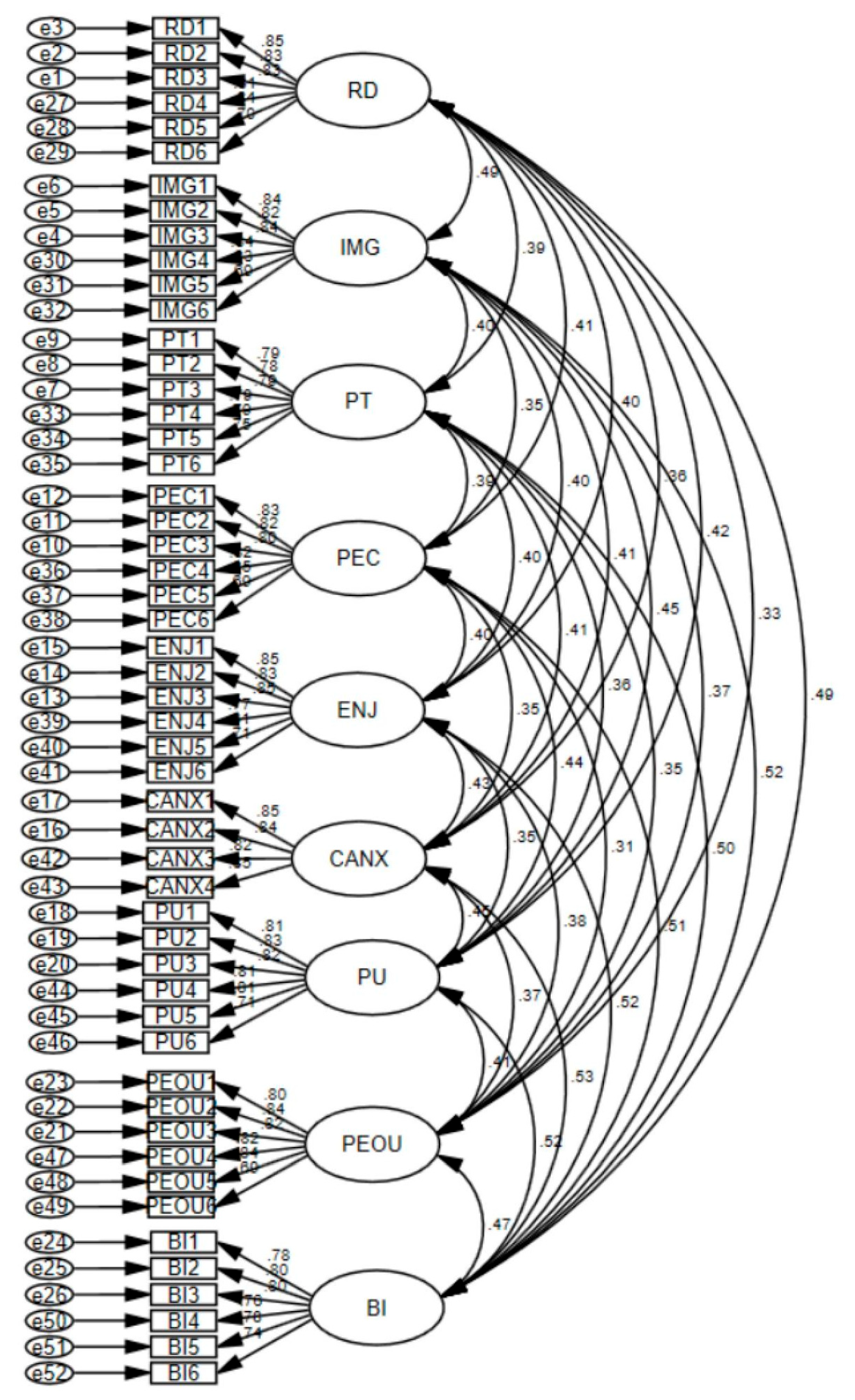
Table 8. Model Fit Indices for Confirmatory Factor Analysis.

Model Fit
Indicator category	The name of the metric	Adaptation criteria	Test results	Acceptable
Absolute fit parameters	GFI	>0.8	0.866	accept
	AGFI	>0.8	0.851	accept
	RMSEA	<0.08	0.015	accept
Value-added suitability parameters	NFI	>0.8	0.89	accept
	IFI	>0.8	0.992	accept
	CFI	>0.8	0.992	accept
	RFI	>0.8	0.882	accept
Simple fit parameters	CMIN/df	<3	1.072	accept
	PGFI	>0.5	0.778	accept

Table 8. Model Fit Indices for Confirmatory Factor Analysis.

Model Fit
Indicator category	The name of the metric	Adaptation criteria	Test results	Acceptable
Absolute fit parameters	GFI	>0.8	0.866	accept
	AGFI	>0.8	0.851	accept
	RMSEA	<0.08	0.015	accept
Value-added suitability parameters	NFI	>0.8	0.89	accept
	IFI	>0.8	0.992	accept
	CFI	>0.8	0.992	accept
	RFI	>0.8	0.882	accept
Simple fit parameters	CMIN/df	<3	1.072	accept
	PGFI	>0.5	0.778	accept

After importing the raw data for analysis, we obtained a series of results. The model fit indices in the table above show that most of the indices meet the acceptable standards. This indicates that the model fits well and that the data we collected can be used for this model. Therefore, the indicators derived from the analysis are reliable for reference.

Table 9. Standardized Factor Loadings from Confirmatory Factor Analysis.

Factor loading coefficient
Factor	Manifest variables	Estimate	S.E.	CR	p	Std. Estimate
RD	RD1	1	-	-	-	0.847
RD	RD2	0.914	0.051	18.05	0.000	0.832
RD	RD3	0.94	0.052	18.013	0.000	0.831
RD	RD4	0.959	0.055	17.372	0.000	0.812
RD	RD5	1.017	0.055	18.431	0.000	0.843
RD	RD6	0.754	0.054	14.077	0.000	0.705
IMG	IMG1	1	-	-	-	0.835
IMG	IMG2	1.007	0.058	17.426	0.000	0.824
IMG	IMG3	0.993	0.055	18.099	0.000	0.844
IMG	IMG4	1.015	0.056	18.028	0.000	0.842
IMG	IMG5	0.953	0.054	17.512	0.000	0.827
IMG	IMG6	0.759	0.056	13.551	0.000	0.692
PT	PT1	1	-	-	-	0.788
PT	PT2	0.975	0.066	14.69	0.000	0.784
PT	PT3	0.963	0.064	14.924	0.000	0.794
PT	PT4	0.96	0.065	14.778	0.000	0.788
PT	PT5	1.011	0.068	14.829	0.000	0.79
PT	PT6	0.864	0.062	13.842	0.000	0.747
PEC	PEC1	1	-	-	-	0.835
PEC	PEC2	1.015	0.059	17.286	0.000	0.823
PEC	PEC3	0.991	0.059	16.711	0.000	0.805
PEC	PEC4	1.004	0.059	17.046	0.000	0.815
PEC	PEC5	1.084	0.059	18.226	0.000	0.852
PEC	PEC6	0.773	0.057	13.483	0.000	0.691
ENJ	ENJ1	1	-	-	-	0.846
ENJ	ENJ2	0.959	0.054	17.739	0.000	0.827
ENJ	ENJ3	1.037	0.056	18.667	0.000	0.853
ENJ	ENJ4	0.879	0.055	15.926	0.000	0.771
ENJ	ENJ5	0.943	0.055	17.14	0.000	0.809
ENJ	ENJ6	0.743	0.053	14.098	0.000	0.708
CANX	CANX1	1	-	-	-	0.846
CANX	CANX2	0.971	0.055	17.632	0.000	0.836
CANX	CANX3	0.914	0.054	16.978	0.000	0.815
CANX	CANX4	0.967	0.054	18.07	0.000	0.85
PU	PU1	1	-	-	-	0.809
PU	PU2	0.99	0.059	16.723	0.000	0.833
PU	PU3	0.968	0.059	16.451	0.000	0.823
PU	PU4	0.966	0.06	15.975	0.000	0.806
PU	PU5	0.922	0.057	16.159	0.000	0.812
PU	PU6	0.768	0.056	13.632	0.000	0.715
PEOU	PEOU1	1	-	-	-	0.801
PEOU	PEOU2	1.065	0.064	16.72	0.000	0.84
PEOU	PEOU3	0.983	0.061	16.131	0.000	0.818
PEOU	PEOU4	1.042	0.064	16.154	0.000	0.819
PEOU	PEOU5	1.07	0.064	16.803	0.000	0.843
PEOU	PEOU6	0.778	0.06	12.875	0.000	0.687
BI	BI1	1	-	-	-	0.777
BI	BI2	1.045	0.071	14.772	0.000	0.796
BI	BI3	1.024	0.069	14.849	0.000	0.8
BI	BI4	0.97	0.069	14.025	0.000	0.763
BI	BI5	0.983	0.068	14.419	0.000	0.78
BI	BI6	0.978	0.072	13.497	0.000	0.738
Note: The horizontal bar ‘-‘ indicates that the item is a reference item.

Table 9. Standardized Factor Loadings from Confirmatory Factor Analysis.

Factor loading coefficient
Factor	Manifest variables	Estimate	S.E.	CR	p	Std. Estimate
RD	RD1	1	-	-	-	0.847
RD	RD2	0.914	0.051	18.05	0.000	0.832
RD	RD3	0.94	0.052	18.013	0.000	0.831
RD	RD4	0.959	0.055	17.372	0.000	0.812
RD	RD5	1.017	0.055	18.431	0.000	0.843
RD	RD6	0.754	0.054	14.077	0.000	0.705
IMG	IMG1	1	-	-	-	0.835
IMG	IMG2	1.007	0.058	17.426	0.000	0.824
IMG	IMG3	0.993	0.055	18.099	0.000	0.844
IMG	IMG4	1.015	0.056	18.028	0.000	0.842
IMG	IMG5	0.953	0.054	17.512	0.000	0.827
IMG	IMG6	0.759	0.056	13.551	0.000	0.692
PT	PT1	1	-	-	-	0.788
PT	PT2	0.975	0.066	14.69	0.000	0.784
PT	PT3	0.963	0.064	14.924	0.000	0.794
PT	PT4	0.96	0.065	14.778	0.000	0.788
PT	PT5	1.011	0.068	14.829	0.000	0.79
PT	PT6	0.864	0.062	13.842	0.000	0.747
PEC	PEC1	1	-	-	-	0.835
PEC	PEC2	1.015	0.059	17.286	0.000	0.823
PEC	PEC3	0.991	0.059	16.711	0.000	0.805
PEC	PEC4	1.004	0.059	17.046	0.000	0.815
PEC	PEC5	1.084	0.059	18.226	0.000	0.852
PEC	PEC6	0.773	0.057	13.483	0.000	0.691
ENJ	ENJ1	1	-	-	-	0.846
ENJ	ENJ2	0.959	0.054	17.739	0.000	0.827
ENJ	ENJ3	1.037	0.056	18.667	0.000	0.853
ENJ	ENJ4	0.879	0.055	15.926	0.000	0.771
ENJ	ENJ5	0.943	0.055	17.14	0.000	0.809
ENJ	ENJ6	0.743	0.053	14.098	0.000	0.708
CANX	CANX1	1	-	-	-	0.846
CANX	CANX2	0.971	0.055	17.632	0.000	0.836
CANX	CANX3	0.914	0.054	16.978	0.000	0.815
CANX	CANX4	0.967	0.054	18.07	0.000	0.85
PU	PU1	1	-	-	-	0.809
PU	PU2	0.99	0.059	16.723	0.000	0.833
PU	PU3	0.968	0.059	16.451	0.000	0.823
PU	PU4	0.966	0.06	15.975	0.000	0.806
PU	PU5	0.922	0.057	16.159	0.000	0.812
PU	PU6	0.768	0.056	13.632	0.000	0.715
PEOU	PEOU1	1	-	-	-	0.801
PEOU	PEOU2	1.065	0.064	16.72	0.000	0.84
PEOU	PEOU3	0.983	0.061	16.131	0.000	0.818
PEOU	PEOU4	1.042	0.064	16.154	0.000	0.819
PEOU	PEOU5	1.07	0.064	16.803	0.000	0.843
PEOU	PEOU6	0.778	0.06	12.875	0.000	0.687
BI	BI1	1	-	-	-	0.777
BI	BI2	1.045	0.071	14.772	0.000	0.796
BI	BI3	1.024	0.069	14.849	0.000	0.8
BI	BI4	0.97	0.069	14.025	0.000	0.763
BI	BI5	0.983	0.068	14.419	0.000	0.78
BI	BI6	0.978	0.072	13.497	0.000	0.738
Note: The horizontal bar ‘-‘ indicates that the item is a reference item.

In terms of measurement relationships, the absolute values of all standardized factor loadings were greater than 0.6 and statistically significant. This means the measurement relationships are strong.

Table 10. AVE and CR Values for Constructs.

Model AVE and CR index results
Factor	AVE	CR
RD	0.661	0.921
IMG	0.660	0.921
PT	0.611	0.904
PEC	0.648	0.917
ENJ	0.646	0.916
CANX	0.701	0.903
PU	0.641	0.914
PEOU	0.645	0.916
BI	0.602	0.901

Table 10. AVE and CR Values for Constructs.

Model AVE and CR index results
Factor	AVE	CR
RD	0.661	0.921
IMG	0.660	0.921
PT	0.611	0.904
PEC	0.648	0.917
ENJ	0.646	0.916
CANX	0.701	0.903
PU	0.641	0.914
PEOU	0.645	0.916
BI	0.602	0.901

As shown in the table above, the AVE values of the nine constructs were 0.661, 0.660, 0.611, 0.648, 0.646, 0.701, 0.641, 0.645, and 0.602. The CR values were 0.921, 0.921, 0.904, 0.917, 0.916, 0.903, 0.914, 0.916, and 0.901. All met the required standards. At the same time, the factor loadings of each item on its corresponding construct were greater than 0.6, showing a strong correspondence between items and constructs. This result indicates that the convergent validity within each construct meets the standard.

After confirming that convergent validity meets the standard, we analysed discriminant validity. The criterion for discriminant validity is that the square root of the AVE on the diagonal should be greater than the Pearson correlation coefficients between constructs.

As shown in the table below, the square root of the AVE for each construct was greater than its correlations with other constructs. This indicates that the discriminant validity of each construct meets the standard. The detailed data are shown in the table below:

Table 11. Discriminant Validity Analysis.

Discriminant validity: Pearson correlation and square root of AVE
	RD	IMG	PT	PEC	ENJ	CANX	PU	PEOU	BI
RD	0.813
IMG	0.446	0.812
PT	0.35	0.355	0.782
PEC	0.37	0.315	0.358	0.805
ENJ	0.365	0.361	0.366	0.379	0.804
CANX	0.324	0.373	0.375	0.328	0.396	0.837
PU	0.379	0.411	0.334	0.399	0.321	0.408	0.801
PEOU	0.308	0.34	0.322	0.285	0.357	0.341	0.376	0.803
BI	0.446	0.467	0.456	0.467	0.479	0.485	0.471	0.429	0.776

Note: The diagonal numbers represent the square root of AVE.

Table 11. Discriminant Validity Analysis.

Discriminant validity: Pearson correlation and square root of AVE
	RD	IMG	PT	PEC	ENJ	CANX	PU	PEOU	BI
RD	0.813
IMG	0.446	0.812
PT	0.35	0.355	0.782
PEC	0.37	0.315	0.358	0.805
ENJ	0.365	0.361	0.366	0.379	0.804
CANX	0.324	0.373	0.375	0.328	0.396	0.837
PU	0.379	0.411	0.334	0.399	0.321	0.408	0.801
PEOU	0.308	0.34	0.322	0.285	0.357	0.341	0.376	0.803
BI	0.446	0.467	0.456	0.467	0.479	0.485	0.471	0.429	0.776

Note: The diagonal numbers represent the square root of AVE.

From the table above:

For RD, the square root of its AVE is 0.813, which is greater than the maximum absolute value of the inter-factor correlation coefficient, 0.446, indicating good discriminant validity.

For IMG, the square root of its AVE is 0.812, greater than the maximum absolute value of the inter-factor correlation coefficient, 0.467, indicating good discriminant validity.

For PT, the square root of its AVE is 0.782, greater than the maximum absolute value of the inter-factor correlation coefficient, 0.456, indicating good discriminant validity.

For PEC, the square root of its AVE is 0.805, greater than the maximum absolute value of the inter-factor correlation coefficient, 0.467, indicating good discriminant validity.

For ENJ, the square root of its AVE is 0.804, greater than the maximum absolute value of the inter-factor correlation coefficient, 0.479, indicating good discriminant validity.

For CANX, the square root of its AVE is 0.837, greater than the maximum absolute value of the inter-factor correlation coefficient, 0.485, indicating good discriminant validity.

For PU, the square root of its AVE is 0.801, greater than the maximum absolute value of the inter-factor correlation coefficient, 0.471, indicating good discriminant validity.

For PEOU, the square root of its AVE is 0.803, greater than the maximum absolute value of the inter-factor correlation coefficient, 0.429, indicating good discriminant validity.

For BI, the square root of its AVE is 0.776, greater than the maximum absolute value of the inter-factor correlation coefficient, 0.485, indicating good discriminant validity.

4.6. Correlation Analysis

Before conducting the correlation analysis, the mean scores of all items belonging to the same construct were used as the indicator for that construct. In SPSS, each construct’s indicator was entered into the variable box for analysis. The results are as follows:

Table 12. Correlation Matrix of Variables.

Pearson Correlation
	RD	IMG	PT	PEC	ENJ	CANX	PU	PEOU	BI
RD	1
IMG	0.446**	1
PT	0.350**	0.355**	1
PEC	0.370**	0.316**	0.359**	1
ENJ	0.365**	0.361**	0.366**	0.378**	1
CANX	0.324**	0.373**	0.374**	0.328**	0.396**	1
PU	0.379**	0.411**	0.334**	0.399**	0.321**	0.408**	1
PEOU	0.308**	0.340**	0.322**	0.285**	0.357**	0.342**	0.377**	1
BI	0.446**	0.467**	0.456**	0.466**	0.479**	0.485**	0.470**	0.429**	1

* p<0.05 ** p<0.01.

Table 12. Correlation Matrix of Variables.

Pearson Correlation
	RD	IMG	PT	PEC	ENJ	CANX	PU	PEOU	BI
RD	1
IMG	0.446**	1
PT	0.350**	0.355**	1
PEC	0.370**	0.316**	0.359**	1
ENJ	0.365**	0.361**	0.366**	0.378**	1
CANX	0.324**	0.373**	0.374**	0.328**	0.396**	1
PU	0.379**	0.411**	0.334**	0.399**	0.321**	0.408**	1
PEOU	0.308**	0.340**	0.322**	0.285**	0.357**	0.342**	0.377**	1
BI	0.446**	0.467**	0.456**	0.466**	0.479**	0.485**	0.470**	0.429**	1

* p<0.05 ** p<0.01.

In summary, the correlations between variables are significant, meeting the prerequisite for analysing influence relationships, so further structural equation modeling can be conducted to verify these relationships.

4.7. AMOS Structural Equation Modeling (Path Analysis and Mediation Analysis)

AMOS 23 software was used to perform SEM analysis. In some studies, it is necessary to handle relationships involving multiple causes and multiple outcomes or to address variables that cannot be directly observed (latent variables), which traditional statistical methods such as correlation or regression cannot adequately resolve. In such cases, SEM is required. First, the theoretical model was used to create a model diagram, as shown below:

Figure 3. Structural Equation Model (SEM) path diagram.

Figure 3. Structural Equation Model (SEM) path diagram.

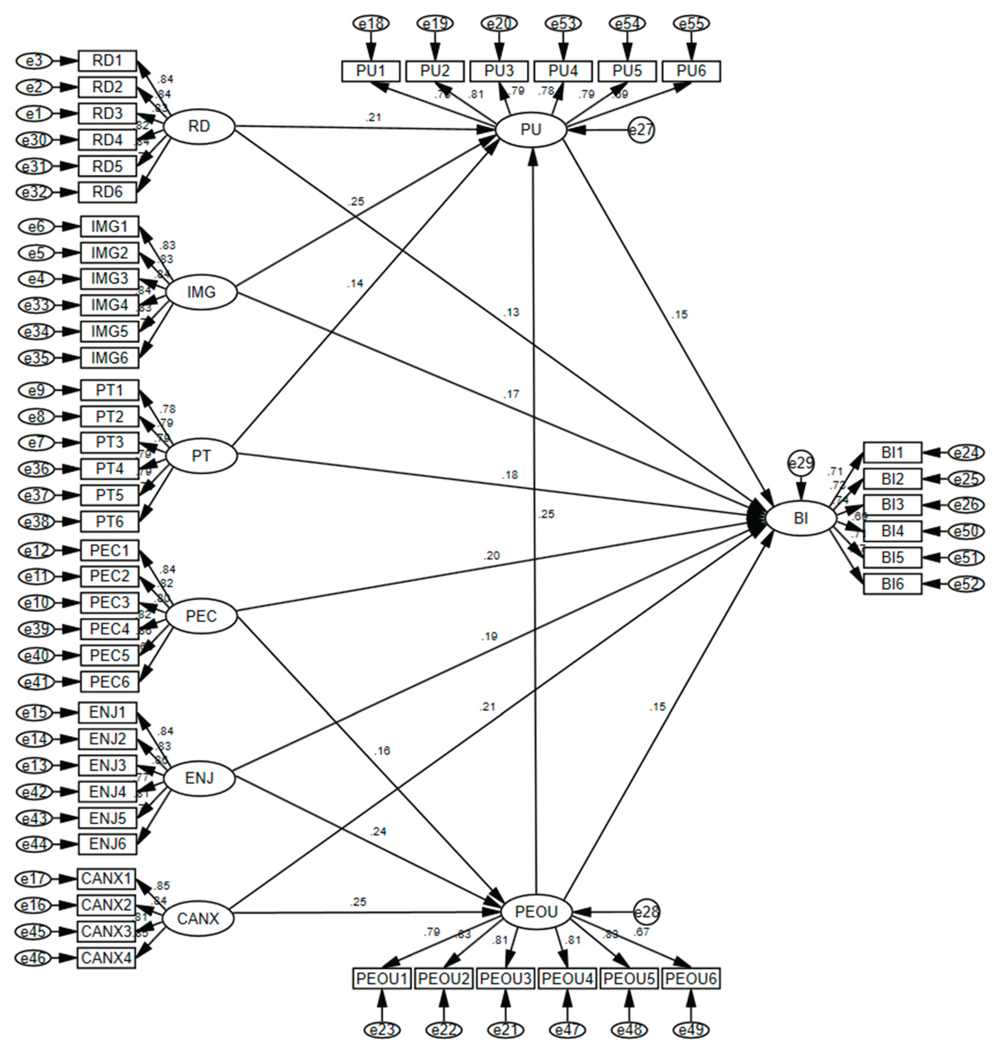
Table 13. Model fit indices and their evaluation.

Model Fit
Indicator category	The name of the metric	Adaptation criteria	Test results	Acceptable
Absolute fit parameters	GFI	>0.8	0.810	accept
	AGFI	>0.8	0.792	accept
	RMSEA	<0.08	0.036	accept
Value-added suitability parameters	NFI	>0.8	0.854	accept
	IFI	>0.8	0.954	accept
	CFI	>0.8	0.954	accept
	RFI	>0.8	0.846	accept
Simple fit parameters	CMIN/df	<5	1.394	accept
	PGFI	>0.5	0.740	accept

Table 13. Model fit indices and their evaluation.

Model Fit
Indicator category	The name of the metric	Adaptation criteria	Test results	Acceptable
Absolute fit parameters	GFI	>0.8	0.810	accept
	AGFI	>0.8	0.792	accept
	RMSEA	<0.08	0.036	accept
Value-added suitability parameters	NFI	>0.8	0.854	accept
	IFI	>0.8	0.954	accept
	CFI	>0.8	0.954	accept
	RFI	>0.8	0.846	accept
Simple fit parameters	CMIN/df	<5	1.394	accept
	PGFI	>0.5	0.740	accept

After importing the raw data for analysis, we obtained a series of results. First, the model fit indices shown in the above table indicate that most of them meet the acceptable standards, suggesting that the model fits well. This means the collected data can be used with this model to estimate the influence relationships among variables, and the results are reliable for reference. Once the model fit was confirmed, the next step was to analyse the influence relationships between variables in detail, as follows:

Table 14. Structural Equation Modeling results table.

SEM Analysis Results
Path	Std.Estimate	Estimate	S.E.	C.R.	P
PEC→PEOU	0.158	0.151	0.056	2.678	0.007
ENJ→PEOU	0.244	0.219	0.054	4.09	***
CANX→PEOU	0.245	0.217	0.053	4.06	***
RD→PU	0.211	0.199	0.055	3.584	***
IMG→PU	0.246	0.224	0.054	4.165	***
PT→PU	0.141	0.148	0.061	2.407	0.016
PEOU→PU	0.252	0.255	0.061	4.209	***
PEOU→BI	0.148	0.116	0.05	2.315	0.021
PU→BI	0.148	0.114	0.049	2.31	0.021
RD→BI	0.133	0.097	0.042	2.307	0.021
IMG→BI	0.166	0.116	0.041	2.831	0.005
PT→BI	0.177	0.143	0.047	3.063	0.002
PEC→BI	0.202	0.151	0.043	3.49	***
ENJ→BI	0.192	0.135	0.041	3.272	0.001
CANX→BI	0.211	0.146	0.041	3.54	***

Table 14. Structural Equation Modeling results table.

SEM Analysis Results
Path	Std.Estimate	Estimate	S.E.	C.R.	P
PEC→PEOU	0.158	0.151	0.056	2.678	0.007
ENJ→PEOU	0.244	0.219	0.054	4.09	***
CANX→PEOU	0.245	0.217	0.053	4.06	***
RD→PU	0.211	0.199	0.055	3.584	***
IMG→PU	0.246	0.224	0.054	4.165	***
PT→PU	0.141	0.148	0.061	2.407	0.016
PEOU→PU	0.252	0.255	0.061	4.209	***
PEOU→BI	0.148	0.116	0.05	2.315	0.021
PU→BI	0.148	0.114	0.049	2.31	0.021
RD→BI	0.133	0.097	0.042	2.307	0.021
IMG→BI	0.166	0.116	0.041	2.831	0.005
PT→BI	0.177	0.143	0.047	3.063	0.002
PEC→BI	0.202	0.151	0.043	3.49	***
ENJ→BI	0.192	0.135	0.041	3.272	0.001
CANX→BI	0.211	0.146	0.041	3.54	***

The above table presents the specific conditions of different paths in the model, including the standardized and unstandardized path coefficients, standard errors, Z-values, and the significance (P-values) of each path. Based on these, the influence relationships among variables can be analysed as follows:

For the path “PEC → PEOU,” the standardized path coefficient is 0.158, reaching the significance level (P<0.05), indicating a significant positive effect.

For the path “ENJ → PEOU,” the standardized path coefficient is 0.244, reaching the significance level (P<0.05), indicating a significant positive effect.

For the path “CANX → PEOU,” the standardized path coefficient is 0.245, reaching the significance level (P<0.05), indicating a significant positive effect.

For the path “RD → PU,” the standardized path coefficient is 0.211, reaching the significance level (P<0.05), indicating a significant positive effect.

For the path “IMG → PU,” the standardized path coefficient is 0.246, reaching the significance level (P<0.05), indicating a significant positive effect.

For the path “PT → PU,” the standardized path coefficient is 0.141, reaching the significance level (P<0.05), indicating a significant positive effect.

For the path “PEOU → PU,” the standardized path coefficient is 0.252, reaching the significance level (P<0.05), indicating a significant positive effect.

For the path “PEOU → BI,” the standardized path coefficient is 0.148, reaching the significance level (P<0.05), indicating a significant positive effect.

For the path “PU → BI,” the standardized path coefficient is 0.148, reaching the significance level (P<0.05), indicating a significant positive effect.

For the path “RD → BI,” the standardized path coefficient is 0.133, reaching the significance level (P<0.05), indicating a significant positive effect.

For the path “IMG → BI,” the standardized path coefficient is 0.166, reaching the significance level (P<0.05), indicating a significant positive effect.

For the path “PT → BI,” the standardized path coefficient is 0.177, reaching the significance level (P<0.05), indicating a significant positive effect.

For the path “PEC → BI,” the standardized path coefficient is 0.202, reaching the significance level (P<0.05), indicating a significant positive effect.

For the path “ENJ → BI,” the standardized path coefficient is 0.192, reaching the significance level (P<0.05), indicating a significant positive effect.

For the path “CANX → BI,” the standardized path coefficient is 0.211, reaching the significance level (P<0.05), indicating a significant positive effect.

4.8. Mediation Effect Test

After the path analysis, it is not possible to directly conclude whether a mediation effect exists. Typically, a more robust analysis method is needed, namely the bootstrap self-sampling method. Next, the bootstrap method will be applied to perform mediation analysis, calculating the 95% confidence interval of a*b to determine the significance of the product term (whether the confidence interval contains zero), thereby determining whether the mediation effect exists.

Table 15. Bootstrap mediation effect results table.

Simple mediating effect test
Path	Effect	Estimate	Lower	Upper	P
RD→PU→BI	Direct effects	0.133	0.004	0.27	0.038
	Indirect effects	0.031	0.005	0.078	0.014
	Total effect	0.164	0.035	0.293	0.011
IMG→PU→BI	Direct effects	0.166	0.011	0.3	0.034
	Indirect effects	0.036	0.008	0.088	0.011
	Total effect	0.202	0.064	0.336	0.006
PT→PU→BI	Direct effects	0.177	0.04	0.31	0.013
	Indirect effects	0.021	0.002	0.058	0.025
	Total effect	0.198	0.063	0.332	0.003
PEC→PEOU→BI	Direct effects	0.202	0.067	0.334	0.004
	Indirect effects	0.023	0.002	0.071	0.027
	Total effect	0.225	0.093	0.354	0.001
ENJ→PEOU→BI	Direct effects	0.192	0.058	0.32	0.009
	Indirect effects	0.036	0.006	0.088	0.016
	Total effect	0.228	0.097	0.359	0.002
CANX→PEOU→BI	Direct effects	0.211	0.072	0.343	0.002
	Indirect effects	0.036	0.006	0.081	0.016
	Total effect	0.248	0.108	0.385	0.001

Table 15. Bootstrap mediation effect results table.

Simple mediating effect test
Path	Effect	Estimate	Lower	Upper	P
RD→PU→BI	Direct effects	0.133	0.004	0.27	0.038
	Indirect effects	0.031	0.005	0.078	0.014
	Total effect	0.164	0.035	0.293	0.011
IMG→PU→BI	Direct effects	0.166	0.011	0.3	0.034
	Indirect effects	0.036	0.008	0.088	0.011
	Total effect	0.202	0.064	0.336	0.006
PT→PU→BI	Direct effects	0.177	0.04	0.31	0.013
	Indirect effects	0.021	0.002	0.058	0.025
	Total effect	0.198	0.063	0.332	0.003
PEC→PEOU→BI	Direct effects	0.202	0.067	0.334	0.004
	Indirect effects	0.023	0.002	0.071	0.027
	Total effect	0.225	0.093	0.354	0.001
ENJ→PEOU→BI	Direct effects	0.192	0.058	0.32	0.009
	Indirect effects	0.036	0.006	0.088	0.016
	Total effect	0.228	0.097	0.359	0.002
CANX→PEOU→BI	Direct effects	0.211	0.072	0.343	0.002
	Indirect effects	0.036	0.006	0.081	0.016
	Total effect	0.248	0.108	0.385	0.001

From the table above,

In the mediation path “RD→PU→BI,” the mediation effect value is 0.031, with a bootstrap confidence interval of 0.005–0.078; since the interval does not include zero, the mediation effect is significant.

In the mediation path “IMG→PU→BI,” the mediation effect value is 0.036, with a bootstrap confidence interval of 0.008–0.088; since the interval does not include zero, the mediation effect is significant.

In the mediation path “PT→PU→BI,” the mediation effect value is 0.021, with a bootstrap confidence interval of 0.002–0.058; since the interval does not include zero, the mediation effect is significant.

In the mediation path “PEC→PEOU→BI,” the mediation effect value is 0.023, with a bootstrap confidence interval of 0.002–0.071; since the interval does not include zero, the mediation effect is significant.

In the mediation path “ENJ→PEOU→BI,” the mediation effect value is 0.036, with a bootstrap confidence interval of 0.006–0.088; since the interval does not include zero, the mediation effect is significant.

In the mediation path “CANX→PEOU→BI,” the mediation effect value is 0.036, with a bootstrap confidence interval of 0.006–0.081; since the interval does not include zero, the mediation effect is significant.

Table 16. Bootstrap mediation effect results table.

Chain mediation effect test
Path	Effect	Estimate	Lower	Upper	P
PEC→PEOU→PU→BI	Direct effects	0.202	0.067	0.334	0.004
	Indirect effects	0.006	0.001	0.021	0.02
	Total effect	0.208	0.073	0.341	0.004
ENJ→PEOU→PU→BI	Direct effects	0.192	0.058	0.32	0.009
	Indirect effects	0.009	0.002	0.027	0.007
	Total effect	0.201	0.066	0.333	0.006
CANX→PEOU→PU→BI	Direct effects	0.211	0.072	0.343	0.002
	Indirect effects	0.009	0.002	0.028	0.008
	Total effect	0.22	0.083	0.351	0.002

Table 16. Bootstrap mediation effect results table.

Chain mediation effect test
Path	Effect	Estimate	Lower	Upper	P
PEC→PEOU→PU→BI	Direct effects	0.202	0.067	0.334	0.004
	Indirect effects	0.006	0.001	0.021	0.02
	Total effect	0.208	0.073	0.341	0.004
ENJ→PEOU→PU→BI	Direct effects	0.192	0.058	0.32	0.009
	Indirect effects	0.009	0.002	0.027	0.007
	Total effect	0.201	0.066	0.333	0.006
CANX→PEOU→PU→BI	Direct effects	0.211	0.072	0.343	0.002
	Indirect effects	0.009	0.002	0.028	0.008
	Total effect	0.22	0.083	0.351	0.002

From the table above,

In the chain mediation path “PEC→PEOU→PU→BI,” the chain mediation effect value is 0.006, with a bootstrap confidence interval of 0.001–0.021; since the interval does not include zero, the chain mediation effect is significant.

In the chain mediation path “ENJ→PEOU→PU→BI,” the chain mediation effect value is 0.009, with a bootstrap confidence interval of 0.002–0.027; since the interval does not include zero, the chain mediation effect is significant.

In the chain mediation path “CANX→PEOU→PU→BI,” the chain mediation effect value is 0.009, with a bootstrap confidence interval of 0.002–0.028; since the interval does not include zero, the chain mediation effect is significant.

5. Conclusions and Discussions

5.1. Conclusions of the Research

Based on the classical Technology Acceptance Model (TAM) and its extended pathways, this study constructed a structural equation model incorporating multiple dimensions of external variables, comprehensively analysing the key factors and mechanisms influencing the acceptance intention of users in China and Europe toward a given technology. Empirical data validation revealed that Perceived Usefulness (PU) and Perceived Ease of Use (PEOU) remain the core variables affecting users’ Behavioral Intention (BI). Both variables exhibited significant positive effects across different cultural contexts, indicating that the classical TAM framework possesses strong theoretical adaptability in cross-cultural settings. Notably, PEOU influences BI not only through a direct path but also indirectly by enhancing PU, further confirming the interactive effects and hierarchical transmission mechanisms between cognitive variables.

To enhance the explanatory power of the model, six external perception variables were introduced into the original framework: *Result Demonstrability* (RD), *Image* (IMG), *Perceived Trust* (PT), *Perceived External Control* (PEC), *Perceived Enjoyment* (ENJ), and *Computer Anxiety* (CANX). The findings show that all these variables significantly affect BI through mediation paths, demonstrating the effectiveness of the extended model in explaining user behavioral motivations. PEC, ENJ, and CANX stand out in particular, as they not only significantly influence PEOU but also exert a direct effect on BI, indicating that users’ sense of control, enjoyment of use, and sensitivity to privacy risks are critical in the technology adoption process. Meanwhile, RD, IMG, and PT mainly affect BI indirectly through PU, highlighting the bridging role of perceived utility in users’ cognitive structures.

Furthermore, mediation and chain mediation effects were tested using the Bootstrap method, which clarified the transmission paths of external variables in the formation of user behavioral intention. The study found that several chain mediation paths—including “PEC→PEOU→PU→BI,” “ENJ→PEOU→PU→BI,” and “CANX→PEOU→PU→BI”—exert significant positive effects, indicating that behavioral intention is jointly shaped by multi-stage cognitive processes. This result supplements the relatively linear and unidirectional limitations of the traditional TAM from a dynamic mechanism perspective, thereby expanding the theoretical complexity of the model.

Based on the path coefficients of the structural equation model and the results of hypothesis testing, all 25 research hypotheses proposed in this study received strong support in both theoretical construction and empirical analysis. The paths associated with Perceived Usefulness (H1–H3, H13–H14) reflect users’ strong recognition of the functional benefits of technology in improving efficiency, reducing accidents, and enhancing environmental quality. Variables related to Perceived Trust (H7–H8) significantly influence PU and BI through reliability expectations, confirming the critical role of trust mechanisms such as legal norms, ethical frameworks, and data security. Perceived External Control (H9–H11) exerts a positive influence on both PEOU and BI, underscoring the importance of policy support, infrastructure, and corporate initiatives. The significant paths between Perceived Enjoyment (H12–H14) and both PEOU and BI indicate that enjoyable experiences have become an important cognitive dimension affecting user acceptance of intelligent transportation technologies. Computer Anxiety (H15–H16) shows significant negative paths that inhibit user willingness to adopt, confirming user sensitivity to uncertainty and lack of control. Other operational hypotheses associated with PU and PEOU (H17–H22) also receive path support, demonstrating that clear guidance, stable operation, and policy coordination in the technology significantly improve overall user acceptance. Finally, the hypotheses under the BI dimension (H23–H25) integrate users’ future adoption intentions, recommendation behaviors, and subjective evaluations of the technology’s superiority, further strengthening the model’s explanatory power for behavioral tendencies. Overall, the path structure among variables not only aligns with the logic of technology acceptance but also statistically illustrates the joint driving mechanism of cognitive, emotional, and institutional variables on user behavior.

In addition, the study found that Chinese and European users showed largely consistent perceptions for most variables, suggesting a strong cross-cultural commonality in the cognitive mechanisms underlying technology acceptance. However, for key indicators such as Behavioral Intention (BI), the average score of Chinese users was slightly higher than that of European users, possibly reflecting greater openness to emerging technologies and stronger trust in technology under policy support in China. This cultural difference suggests that in global technology promotion, strategies should be tailored to local conditions, taking into account cultural environments, cognitive preferences, and policy contexts to enhance adaptability. Finally, from the perspective of model evaluation, the structural equation model constructed in this study demonstrated good fit (e.g., CFI = 0.954, RMSEA = 0.036), and the reliability, convergent validity, and discriminant validity of all measurement dimensions met both theoretical and statistical standards, indicating a reasonable model structure, high data quality, and robust, interpretable results. The research not only verifies the robustness of the TAM in cross-cultural contexts but also, through the integration of external variables and the decomposition of path mechanisms, provides a more systematic theoretical perspective and practical foundation for understanding the formation of user behavioral intentions.

5.2. Theoretical Significance

This study adopts the classical Technology Acceptance Model (TAM) as its theoretical framework and, drawing on the realities of autonomous driving development in China and Europe, constructs a public acceptance model that integrates multidimensional variables such as technological cognition, institutional trust, and social value recognition. This enriches the explanatory pathways of TAM in high-risk and emerging technology contexts. By introducing TAM into the field of autonomous driving—a complex, emerging technology that combines artificial intelligence, algorithmic control, ethical decision-making, and legal responsibility—this study empirically tests whether Perceived Usefulness (PU) and Perceived Ease of Use (PEOU) remain the fundamental drivers of adoption behavior, while further verifying TAM’s extensibility and practical adaptability. The research trajectory from “functional benefits” toward “institutional recognition” and “ethical alignment” expands the theoretical boundaries of TAM.

The extended variables introduced in this study—Result Demonstrability (RD), Image (IMG), Perceived Trust (PT), Perceived External Control (PEC), Perceived Enjoyment (ENJ), and Computer Anxiety (CANX)—demonstrate that, when facing a high-complexity, high-perceived-risk technology such as autonomous driving, users’ decision-making foundations are no longer solely based on functional judgments. Instead, they also include comprehensive evaluations of institutional context, ethical expectations, and technological trust. This cognition–emotion–institution coupling provides empirical grounding for extending TAM from a “tool-rationality perspective” to a “social–cultural–emotional–value cognition synergy perspective,” responding to current theoretical calls in emerging technology acceptance research regarding “bounded rationality,” “contextual relevance,” and “institutional moderation”.

In addition, this study focuses on China and Europe—two regions with significant differences in institutional contexts, technological development status, and cultural traditions—and constructs a cross-cultural comparative pathway based on a unified measurement scale. By comparing public acceptance of autonomous driving technology in these different institutional and cultural contexts, it empirically verifies the moderating effects of institutional trust, policy orientation, and ethical cognition in technology adoption. This structural comparison not only enhances TAM’s cross-cultural adaptability but also provides theoretical support for future explorations of the dynamic interaction between global technology diffusion and local cognition. It fills the gap in current autonomous driving acceptance research where structured China–Europe comparisons are scarce, and it verifies the similarities and differences in the performance of technological cognition variables across cultures. The parameter structure, measurement tools, and analytical model developed here demonstrate strong adaptability, offering theoretical references and operational paradigms for subsequent public acceptance studies in other high-technology fields such as AI-assisted medical diagnosis, unmanned delivery, and intelligent algorithm platforms.

In summary, the main theoretical contributions of this study are:(1) Introducing TAM for the first time in a systematic way into the autonomous driving context, integrating it with variables related to institutions, emotions, and social recognition to construct an acceptance pathway model. (2) Enhancing the practical adaptability of TAM in complex technological environments through standardized variable substitution and model modification. (3) Expanding the cross-cultural theoretical explanatory scope of TAM through a comparative approach.These theoretical contributions lay a solid foundation for future research on the social embedding of emerging technologies such as autonomous driving and provide a structural analytical framework for understanding the evolution mechanisms of public attitudes toward technology.

5.3. Limitations and Future Directions

Although this study has made certain explorations in theoretical modeling and empirical analysis, it still has the following limitations that require further improvement in future research. First, in terms of sample composition and acquisition methods, although the study covered representative respondents from both China and Europe, limitations in research resources and online dissemination channels led to a certain degree of imbalance in sample distribution. The data were collected through a questionnaire survey, and although the respondents represented populations from both China and Europe, restrictions in survey timing and resource allocation resulted in an incomplete balance of sample distribution. In addition, the proportions of age and gender were relatively concentrated, which may have affected the generalizability of the conclusions and influenced the results of cross-cultural comparisons.

Second, regarding variable construction and design, although this study strived to align each parameter precisely with the issue of autonomous driving acceptance, there remains a certain degree of abstraction and insufficient explanatory power. For example, parameters such as institutional trust or legal–ethical relevance were theoretically integrated into “facilitating conditions” or “perceived external control,” but in the actual questionnaire, respondents may not have clearly distinguished between dimensions such as “institutional safeguards,” “technological transparency,” and “data security,” leading to potential semantic bias in measurement results.

Third, the research findings have certain temporal limitations. Since autonomous driving technology is still in a stage of rapid global development intertwined with social controversy, public perceptions are not yet stable and are easily influenced by factors such as media coverage, policy directions, and accident-related public opinion. The data collection phase of this study coincided with the promotion of autonomous driving pilot programs in multiple Chinese and European cities, while related accidents were also widely reported during the same period. As a result, respondents may have combined rational judgments with emotional reactions when answering, which could affect the stability of the data. Repeated testing at different stages in the future may lead to different conclusions.

In summary, although this study has made breakthroughs in theoretical construction and cross-cultural empirical research, it is still subject to multiple limitations in terms of sample representativeness, parameter accuracy, and the influence of non-rational factors. Subsequent research should explore public acceptance of autonomous driving among broader populations, with more diverse theoretical perspectives and more dynamic methodological frameworks.

Based on the above limitations, future research can be expanded in the following directions. First, it is recommended to further broaden the sample coverage by increasing the proportion of respondents from different countries, cities, and social backgrounds, particularly by incorporating more representative user groups such as older adults and women. This would enrich respondent profiles and enhance the explanatory power and generalizability of the findings across diverse groups.

Second, future research is encouraged to adopt a longitudinal tracking design to observe the evolution of public acceptance across different stages of technological development through time-series analysis. By incorporating typical events (e.g., major accidents, policy shifts, or technological upgrades), researchers can conduct causal pathway analyses to explore the dynamic mechanisms underlying public attitudes. Monitoring the temporal evolution of acceptance can help identify critical turning points during technology maturation, before and after major incidents, and in moments of policy change.

Third, future studies could integrate experimental simulations with real-world experiences, allowing respondents to personally engage with autonomous driving systems in a controlled environment. By examining behavioral observations, electroencephalography (EEG) signals, heart rate responses, and other physiological measures, researchers can gain deeper insights into the cognitive and emotional mechanisms underlying user acceptance, thereby advancing autonomous driving acceptance research from the “perceptual level” to the “behavioral level” and the “decision-making mechanism level”.

Finally, the cultural dimension remains an important area for future exploration. Although this study conducted cross-cultural analysis through a China–Europe comparison, the measurement of cultural values remained at a relatively surface level, treating regional cultural differences merely as observational variables. Future research could further investigate how different cultural contexts—such as regional culture, occupational culture, and technology-community culture—affect acceptance levels of autonomous driving, thereby constructing a more nuanced cultural explanatory framework.

References

- General Office of the State Council. (2024, November 1). Notice on the latest regulations for optimizing the business environment. Central People’s Government of the People’s Republic of China. https://www.gov.cn/yaowen/liebiao/202411/content_6986907.htm.
- CPCA auto market news. (n.d.). China Passenger Car Association. http://www.cpcaauto.com/newslist.php?types=csjd&id=3553.
- State Council, PRC. (2025, January 15). Illustrated interpretation of measures to optimize the business environment. Central People’s Government of the People’s Republic of China. https://www.gov.cn/zhengce/jiedu/tujie/202501/content_6999527.htm.
- IEA (2024), Global EV Outlook 2024, IEA, Paris https://www.iea.org/reports/global-ev-outlook-2024, Licence: CC BY 4.0.
- Autovista Group. (2025). Which brand sold the most EVs in Europe in 2024?. Autovista24. https://autovista24.autovistagroup.com/news/which-brand-sold-the-most-evs-in-europe-in-2024/.
- European Commission. (2024). Sustainable and Smart Mobility Strategy – putting European transport on track for the future. Directorate-General for Mobility and Transport. https://transport.ec.europa.eu/transport-themes/mobility-strategy_en.
- European Parliament. (2022). EU ban on sale of new petrol and diesel cars from 2035 explained. https://www.europarl.europa.eu/topics/en/article/20221019STO44572/eu-ban-on-sale-of-new-petrol-and-diesel-cars-from-2035-explained.
- McCauley, R. Why autonomous and electric vehicles are inextricably linked. GovTech. https://www.govtech.com/fs/why-autonomous-and-electric-vehicles-inextricably-linked.html.
- Zhang, Y. (2025, April 2). Xiaomi auto denies claims spontaneous combustion caused fire in fatal SU7 car crash. Yicai Global. https://www.yicaiglobal.com/news/xiaomi-auto-denies-claims-spontaneous-combustion-caused-fire-in-fatal-su7-car-crash.
- Ren, D. (2025, April 1). Xiaomi to cooperate with police after fatal crash involving SU7 EV’s self-driving feature. South China Morning Post. https://www.scmp.com/business/china-business/article/3304794/xiaomi-cooperate-police-after-fatal-crash-involving-su7-evs-self-driving-feature.
- China News Service. (2025, April 1). [Five questions about Xiaomi SU7 explosion accident]. China News Network. https://www.chinanews.com.cn/cj/2025/04-01/10393099.shtml.
- Wang, M. A. (2024). Research on influencing factors of continuous intention of autonomous driving technology [Master’s thesis, Beijing University of Posts and Telecommunications]. CNKI. [CrossRef]
- Alqahtani, T. Recent Trends in the Public Acceptance of Autonomous Vehicles: A Review. Vehicles 2025, 7, 45. [Google Scholar] [CrossRef]
- Cui, L.Y. & Bu, W.J. Autonomous driving: China leads global acceptance. China Strategic Emerging Industry 2018, 78–79. [Google Scholar] [CrossRef]
- J.D. Power & Global Times. (2021, May). China consumer autonomous vehicle confidence index survey. J.D. Power China. from https://china.jdpower.com/sites/china/files/file/2021-05/中国消费者自动驾驶信心指数调查_JDPower(君迪)与《环球时报》联合发布_202105.pdf.
- BUSINESS SWEDEN. (2024). HOW CHINA IS SHAPING THE AUTONOMOUS DRIVING INDUSTRY— A study on trends and driving forces reshaping the world’s largest automotive market. Trafikanalys (Trafa). from https://www.trafa.se/globalassets/rapporter/underlagsrapporter/2025/study-on-chinas-autonomous-vehicles-and-auto-driving-system.pdf.
- Xinhua News Agency. (2023). Over 40% of new passenger cars in China equipped with combined driving assistance functions. The State Council of the People’s Republic of China. https://www.gov.cn/lianbo/bumen/202309/content_6905530.htm.
- Wei, X.X. , & Zhong, S.Q. Understanding the Acceptance Intentions of Automated Vehicles Based on TAM and Cognitive Theory. CHINA TRANSPORTATION REVIEW 2019, 41, 79–84. [Google Scholar]
- Tang, L. , Qing, S. D., Xu, Z. G., & Zhou, H. Q. Research review on public acceptance of autonomous driving. Journal of Traffic and Transportation Engineering 2020, 20, 131–146. [Google Scholar] [CrossRef]
- QIN, H. , ZHANG, R., & WANG, P. The Differences in User Acceptability of Autonomous Vehicles between China and the United States. Science Technology and Engineering 2021, 21, 6487–6493. [Google Scholar]
- Wan, D. , & Peng, L. Autonomous Vehicle Acceptance in China: TAM-Based Comparison of Civilian and Military Contexts. World Electric Vehicle Journal 2025, 16, 2. [Google Scholar] [CrossRef]
- National Development and Reform Commission (NDRC). (2020). Intelligent vehicle innovation and development strategy. National Development and Reform Commission. Retrieved July 1, 2025, from https://www.ndrc.gov.cn/xxgk/zcfb/tz/202002/P020200224573058971435.pdf.
- Ministry of Transport of the People’s Republic of China. (2020). Guiding opinions on promoting the development and application of road traffic autonomous driving technology (Document No. Jiao Ke Ji Fa [2020] No. 124). Central People’s Government of the People’s Republic of China. Retrieved July 2, 2025, from https://www.gov.cn/zhengce/zhengceku/2020-12/30/content_5575422.htm.
- Schoettle, B. , & Sivak, M. (2014). Public opinion about self-driving vehicles in China, India, Japan, the US, the UK, and Australia. Ann Arbor, MI: The University of Michigan.
- Nordhoff, S. , de Winter, J, , Kyriakidis, M., van Arem, B., & Happee, R. Acceptance of driverless vehicles: Results from a large cross-national questionnaire study. Journal of Advanced Transportation 2018, 2018, 5382192. [Google Scholar] [CrossRef]
- Anania, E. C. , Rice, S, Walters, N. W., Pierce, M., Winter, S. R., & Milner, M. N. The effects of positive and negative information on consumers’ willingness to ride in a driverless vehicle. Transport Policy 2018, 72, 218–224. [Google Scholar] [CrossRef]
- Hudson, J. , Orviska, M, & Hunady, J. People’s attitudes to autonomous vehicles. Transportation Research Part A: Policy and Practice 2019, 121, 164–176. [Google Scholar]
- dos Santos, F. L. M. , Duboz, A, Grosso, M., Raposo, M. A., Krause, J., Mourtzouchou, A., Balahur, A., & Ciuffo, B. An acceptance divergence? Media, citizens and policy perspectives on autonomous cars in the European Union. Transportation Research Part A: Policy and Practice 2022, 158, 224–238. [Google Scholar] [CrossRef] [PubMed]
- European Commission. (2018). On the road to automated mobility: An EU strategy for mobility of the future (COM(2018)0283). Brussels: European Commission.
- European Parliament. (2019). Resolution on autonomous driving in European transport (2018/2089(INI)). Official Journal of the European Union, C 411/1–20.
- European Parliament. (2019, ). Self-driving cars in the EU: From science fiction to reality. European Parliament News. Retrieved July 2, 2025, from https://www.europarl.europa.eu/topics/en/article/20190110STO23102/self-driving-cars-in-the-eu-from-science-fiction-to-reality.
- Salonen, A. O. Passenger’s subjective traffic safety, in-vehicle security and emergency management in the driverless shuttle bus in Finland. Transport Policy 2018, 61, 106–110. [Google Scholar] [CrossRef]
- Burke, F. (2021). Do you trust automated cars? If not, you’re not alone. Horizon: The EU Research & Innovation Magazine. Retrieved , 2025, from https://projects.research-and-innovation.ec.europa.eu/en/horizon-magazine/do-you-trust-automated-cars-if-not-youre-not-alone.
- Hajjafari, H. (2018). Exploring the effects of socio-demographic and built environmental factors on the public adoption of shared and private autonomous vehicles: A case study of Dallas-Fort Worth metropolitan area [Doctoral dissertation, University of Texas at Arlington]. Public Affairs Dissertations. https://mavmatrix.uta.edu/publicaffairs_dissertations/171/.
- Adnan, N. , Nordin, SM., bin Baharuddin, M. A., & Ali, M. How trust can drive forward the user acceptance to the technology? In-vehicle technology for autonomous vehicle. Transportation Research Part A: Policy and Practice 2018, 118, 819–836. [Google Scholar] [CrossRef]
- European Parliamentary Research Service. (2018). A common EU approach to liability rules and insurance for connected and autonomous vehicles (EPRS Study, PE 615.635). European Parliament.
- Zhu, J. W. Risks and Challenges of China’s New Energy Vehicles Going Overseas under the EU’s New Automotive Industry Regulations. E-Commerce Letters 2025, 14, 1848–1854. [Google Scholar] [CrossRef]
- European Parliamentary Research Service. (2021). Sustainable and smart mobility strategy. European Parliament. Retrieved July 3, from https://www.europarl.europa.eu/RegData/etudes/BRIE/2021/659455/EPRS_BRI(2021)659455_EN.pdf.
- European Commission. Net-Zero Industry Act: Accelerating the transition to climate neutrality. European Commission. Retrieved July 2 2023, 2025, from https://single-market-economy.ec.europa.eu/industry/sustainability/net-zero-industry-act_en.
- Pangarkar, T. (2025). Autonomous Vehicles Statistics 2025 By Type, Technology, Driving. Market.us News. Retrieved , from https://www.news.market.us/autonomous-vehicles-statistics.
- Davis, F. D. Perceived Usefulness, Perceived Ease of Use, and User Acceptance of Information Technology. MIS Quarterly 1989, 13, 319–340. [Google Scholar] [CrossRef]
- Wu, Z. , Zhou, H, Xi, H., & Wu, N. Analysing public acceptance of autonomous buses based on an extended TAM model. IET Intelligent Transport Systems 2021, 15, 1318–1330. [Google Scholar] [CrossRef]
- Geldmacher, W. , Just, V., Kopia, J., & Kompalla, A. (2017). Development of a modified technology acceptance model for an innovative car sharing concept with self-driving cars. BASIQ 2017 - New Trends in sustainable Business and ConsumptionAt: Graz, AustriaVolume: 1. https://www.researchgate.net/publication/317339694_Development_of_a_modified_technology_acceptance_model_for_an_innovative_car_sharing_concept_with_self-driving_cars.
- Hutchins, N. , & Hook, L. (2017). Technology acceptance model for safety critical autonomous transportation systems. 2017 IEEE/AIAA 36th Digital Avionics Systems Conference (DASC), 1-5. [CrossRef]
- Fiorini, P. de C, Seles, B. M. R. P., Jabbour, C. J. C., Mariano, E. B., & Jabbour, A. B. L. de S. Management theory and big data literature: From a review to a research agenda. International Journal of Information Management 2018, 43, 112–129. [Google Scholar] [CrossRef]
- Aljarrah, E. , Elrehail, H, & Aababneh, B. E-voting in Jordan: Assessing readiness and developing a system. Computers in Human Behavior 2016, 63, 860–867. [Google Scholar] [CrossRef]
- Ajzen, I. The theory of planned behavior. Organizational Behavior and Human Decision Processes 1991, 50, 179–211. [Google Scholar] [CrossRef]
- Venkatesh, V. , Morris, MG., Davis, G. B., & Davis, F. D. User Acceptance of Information Technology: Toward a Unified View. MIS Quarterly 2003, 27, 425–478. [Google Scholar] [CrossRef]
- Yap, M. D. , Correia, G, & van Arem, B. Valuation of travel attributes for using automated vehicles as egress transport of multimodal train trips. Transportation Research Procedia 2015, 10, 462–471. [Google Scholar]
- gini, M. (2022, ). Environmental pros and cons of self-driving cars. Earth.Org. Retrieved July 1, 2025, from https://earth.org/pros-and-cons-of-self-driving-cars/.
- Mu, J. , Zhou, L., & Yang, C. Research on the Behavior Influence Mechanism of Users’ Continuous Usage of Autonomous Driving Systems Based on the Extended Technology Acceptance Model and External Factors. Sustainability 2024, 16, 9696. [Google Scholar] [CrossRef]
- Ro, Y. Ha, Y. A factor analysis of consumer expectations for autonomous cars. Journal of Computer Information Systems 2019, 59, 52–60. [Google Scholar] [CrossRef]
- Dong, X. , DiScenna, M. , & Guerra, E. Transit user perceptions of driverless buses. Transportation 2017, 46, 35–50. [Google Scholar]
- Deichmann, J. Ebel, E., Heineke, K., Heuss, R., Kellner, M., & Steiner, F. (2023). Autonomous driving’s future: Convenient and connected. McKinsey & Company. Retrieved July 5, 2025, from https://www.mckinsey.com/industries/automotive-and-assembly/our-insights/autonomous-drivings-future-convenient-and-connected.
- Rogers, S. (2018). The autonomous car is the next entertainment frontier. Forbes. Retrieved July 4, 2025, from https://www.forbes.com/sites/solrogers/2018/12/12/the-autonomous-car-is-the-next-entertainment-frontier/.
- Xu, Z. , Zhang, K, Min, H., Wang, Z., Zhao, X., & Liu, P. What drives people to accept automated vehicles? Findings from a field experiment. Transportation Research Part C: Emerging Technologies 2018, 95, 320–334. [Google Scholar] [CrossRef]
Disclaimer/Publisher’s Note: The statements, opinions and data contained in all publications are solely those of the individual author(s) and contributor(s) and not of MDPI and/or the editor(s). MDPI and/or the editor(s) disclaim responsibility for any injury to people or property resulting from any ideas, methods, instructions or products referred to in the content. |
© 2025 by the authors. Licensee MDPI, Basel, Switzerland. This article is an open access article distributed under the terms and conditions of the Creative Commons Attribution (CC BY) license (http://creativecommons.org/licenses/by/4.0/).
Copyright: This open access article is published under a Creative Commons CC BY 4.0 license, which permit the free download, distribution, and reuse, provided that the author and preprint are cited in any reuse.