

Submitted:
14 August 2025
Posted:
18 August 2025
You are already at the latest version
Abstract
This paper introduces and computationally analyzes a modified version of the Hala attractor as a chaotic system designed to bridge the gap between dissipative and Hamiltonian dynamics. The model incorporates a tunable dissipation parameter, δ, and an external periodic forcing term to simulate resonance in physical plasma systems. Through numerical simulations and a detailed analysis of Lyapunov exponents and phase space trajectories, it was demonstrated that the system's chaoticity and dissipative properties can be independently controlled. It is shown that the system can transition from a non-chaotic, dissipative state to a chaotic, non-dissipative (Hamiltonian-like) state. This novel approach provides a framework for modeling phenomena in plasma physics, such as wave-particle interactions and collective behavior, where the degree of chaos is not an inherent property but a controllable variable. The findings validate the utility of tunable chaotic systems for advanced applications in engineered chaotic processes.
Keywords:
hala attractor
; hamiltonia systems
; chaos engineering
; plasma physics
1. Introduction
The study of chaotic systems is fundamental to understanding complex, nonlinear phenomena, but it is crucial to distinguish between two primary forms of chaos: Hamiltonian and dissipative. Hamiltonian chaos arises in systems where energy is conserved, and where phase space volume is preserved as trajectories evolve. This is particularly relevant to magnetic confinement systems, such as tokamaks and stellarators, where particle motion is largely governed by electromagnetic fields and total energy is presumed conserved. A classic mechanism for the onset of chaos in these systems is “resonance overlap”, where a particle’s motion resonates with multiple waves simultaneously. This process breaks down regular motion, leading to particle diffusion and is vital for understanding phenomena like plasma heating [1,2,3]. In contrast, dissipative chaos occurs in systems where energy is lost. Here, phase space volume contracts over time, often leading to the formation of strange attractors—which are fractal structures in phase space toward which the system’s trajectory is drawn. While not the primary framework for analyzing core particle trajectories in ideal, collisionless plasma devices, this type of chaos is relevant for certain instabilities or when considering plasma-wall interactions where dissipation is significant. Early models, such as the cold-plasma model, provided also an accurate description of small-amplitude perturbations in a hot plasma [4]. This model captures the collective behavior of plasma waves because their dynamics are primarily driven by the inertial response of charged particles to the wave’s fields, not by random thermal motion. However, that model intentionally neglects individual particle motion and the effects of dissipation, leaving a gap in understanding how energy loss and individual particle dynamics influence a system’s transition to chaos. To address this gap, a new dynamic model is proposed here and that is based on the so—called Hala attractor [5]. Two key modifications are introduced here: first, a tunable parameter, δ, representing a collision frequency that explicitly models the dissipation of energy. This term acts as a friction term that causes phase space volume to contract over time, which is a defining characteristic of dissipative systems. By tuning δ, the system’s behavior changes can be explored as the level of “collisions” is increased or decreased. Then, a second sinusoidal forcing term is added to model resonance overlap. By tuning the frequencies and amplitudes of these forcing terms, the transition from stable periodic motion to chaos as the resonances overlap can be observed. This approach uses the Hala attractor as a base system to study the effects of dissipation and external drivers, moving the analysis from an idealized model of collective wave behavior to a more realistic model that includes the statistical effects of particle interactions.
2. The Modified Hala Attractor Model
To explore the interplay between dissipation and resonance, the research will be based on a modified version of the Hala attractor. The original Hala attractor, inspired by the Lorenz system, is defined by the following system of non-linear ordinary differential equations:
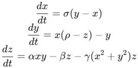
In this formulation, σ, ρ, and β are the classic Lorenz parameters, while α is a chaos-tuning parameter. The term −γ(x2+y2) z is a built-in, self-regulating mechanism where γ serves as a feedback parameter. This term acts as a negative feedback loop that constrains the phase space volume of the attractor as the trajectory expands. The original research that developed the Hala attractor main finding was that the level of chaos, as measured by the largest Lyapunov exponent, is a continuous function of this parameter, allowing for a controlled transition from a chaotic state to a stable fixed point.
2.1. Modifications for Tunable Dissipation and Resonance
To investigate the physical mechanisms of physical plasma heating and chaotic transitions, two key modifications to this base system are introduced:
- Tunable linear dissipation: the original, non-linear feedback term is replaced with a simpler, linear dissipation term. This is motivated by the need to model the effects of collisions in a more direct, tunable manner. A new parameter, δ, is introduced representing a generic damping or collision frequency.
- External periodic forcing: To model the effect of external waves, a time-dependent, sinusoidal forcing term is added to one of the equations. This allows for the study of the effects of resonance and resonance overlap, which are central to the onset of chaos in Hamiltonian systems.
With these modifications, the normalized equations for the modified Hala attractor become:
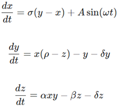
In these equations, A is the amplitude of the external driving wave, and ω is its normalized frequency. The linear dissipation parameter δ directly controls the system’s energy loss. Standard normalizations for plasma systems are used, where the electron plasma frequency (ωp) is the normalizing frequency and the Debye length (λD) is the normalizing length.
2.2. The Dissipative-to-Hamiltonian Transition
A fundamental property of a dynamical system is its divergence, ∇⋅V, which quantifies the rate of phase space volume contraction. For our modified system, the divergence is calculated as:

This equation reveals the central mechanism followed here. The system is dissipative when ∇⋅V<0, which occurs when δ > − (σ+β+1)/2. When the dissipation parameter is set to the critical value δc= − (σ+β+1)/2, the divergence becomes zero. In this state, the phase space volume is conserved, and the system behaves as a non-dissipative, Hamiltonian—like system. This provides a direct, tunable mechanism to bridge the transition gap between dissipative and Hamiltonian chaos.
3. Computational Analysis
The goal in this section is to computationally analyze the system’s behavior as key parameters are systematically varied, particularly the dissipation parameter δ and the driving frequency ω. The standard Lorenz parameters σ=10, ρ=28, and β=8/3, and fix α=1 will be used for this analysis. The computational plan is divided into three parts:
- Baseline simulation (Chaotic dissipative state): First, a baseline will be established by setting δ to a small, positive value (e.g., δ=0.1) and the forcing term to a small amplitude (A=0.1) with a frequency that is not at a resonance. A long simulation is run to allow the system to settle onto its strange attractor, visualize its trajectory in 3D phase space, and calculate its Lyapunov exponents to confirm its chaotic nature.
- Exploring resonance (changing ω): With δ fixed at the chaotic baseline value, the driving frequency ω is systematically varied across a range of values. For each ω, the system’s response is analyzed. It was expected to see a significant change in the system’s behavior when ω matches a natural frequency of the attractor, and a plot of the amplitude of the system’s response as a function of ω to identify these resonances.
- The transition to Hamiltonian system—like behavior (changing δ): Finally, the transition from dissipative to non-dissipative behavior is investigated. With the driving frequency ω fixed at a resonance that has been identified, a series of simulations is run, slowly decreasing the value of δ toward its critical value, δc. The strange attractor was expected to “unfurl” and occupy a larger phase space volume as δ → δc. Concurrently, the sum of Lyapunov exponents at each step was calculated, which was expected to approach zero as the system transitions toward the Hamiltonian-like behavior. This systematic approach provides a clear roadmap for exploring the interplay between dissipation, resonance, and chaos in the modified system.
4. Results and Discussion
The computational analysis outlined in the previous section was executed to test the model’s key theoretical predictions. The findings, presented in a series of key figures, confirm that the modified Hala attractor successfully bridges the concepts of dissipative and Hamiltonian chaos by allowing for a tunable transition between the two regimes while maintaining a chaotic state.
4.1. Dissipation Sweep Analysis
The dissipation sweep, where the parameter δ was systematically varied, yielded three critical plots that collectively prove the model’s behavior.
- Phase space trajectories In Figure 1 the trajectory begins in a deep blue color, corresponding to a state with significant dissipation. As the simulation progresses and the dissipation parameter decreases, the trajectory color transitions to a lighter blue and then to cyan. This change highlights the “unfurling” of the strange attractor, where the system expands its spatial extent as it approaches a non-dissipative state. This plot serves as a clear visual confirmation of the inverse relationship between the dissipation parameter and the volume occupied by the chaotic attractor.
Figure 1.
This figure provides a focused view of the attractor’s “unfurling,” with the trajectory transitioning from a compact state (blue) to an expanded, volume-filling state (cyan) as the dissipation parameter decreases.
Figure 1.
This figure provides a focused view of the attractor’s “unfurling,” with the trajectory transitioning from a compact state (blue) to an expanded, volume-filling state (cyan) as the dissipation parameter decreases.
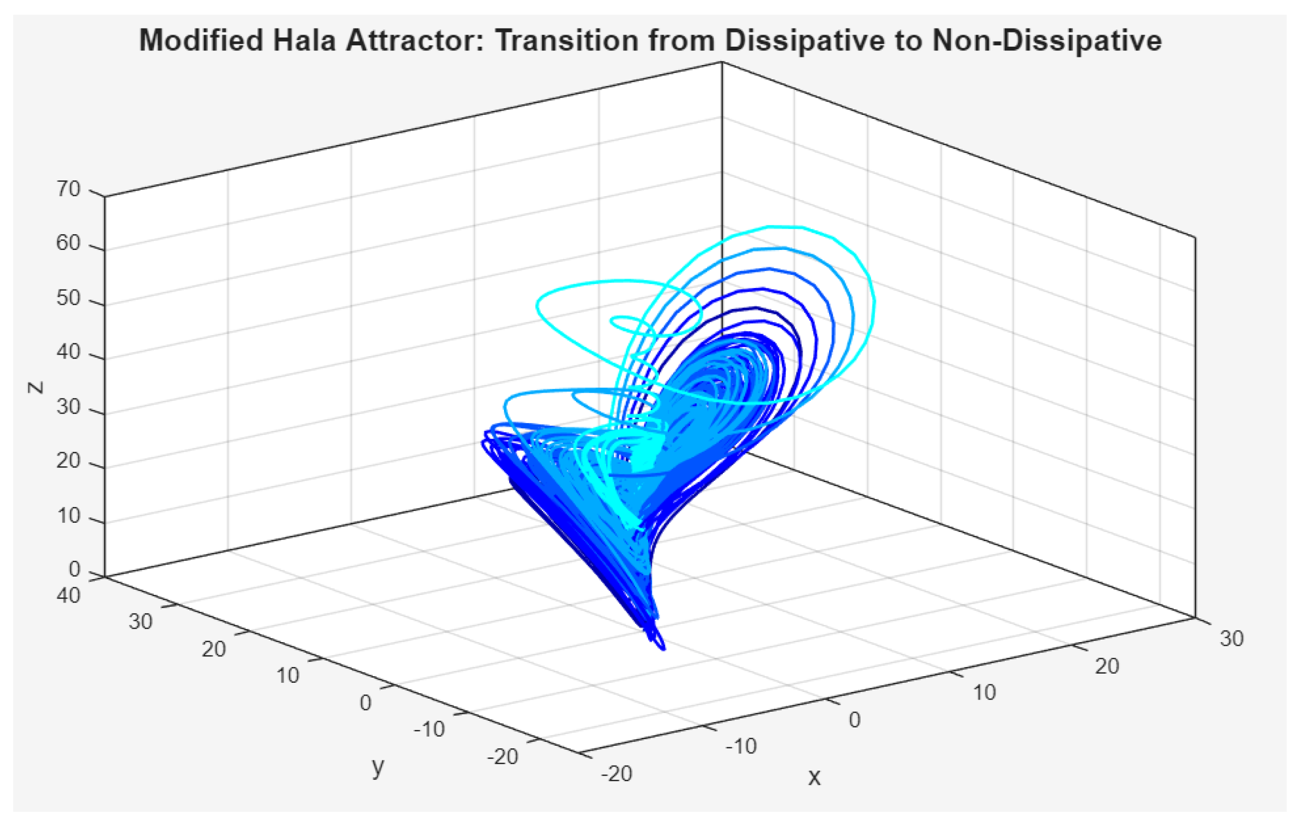
Figure 2 presents a single, continuous trajectory colored by the dissipation parameter, δ, as it is swept from a high positive value (red) to a low one (blue). The red and yellow sections of the trajectory represent the system in a highly dissipative regime, where energy loss is significant and the system is being drawn toward a compact attractor. As the parameter is decreased, the trajectory color shifts to cyan and then to a deeper blue, indicating a reduction in dissipation. This transition visually demonstrates the core concept of the modified Hala attractor model: as the rate of energy loss decreases, the chaotic attractor “unfurls” and expands to occupy a larger phase space volume.
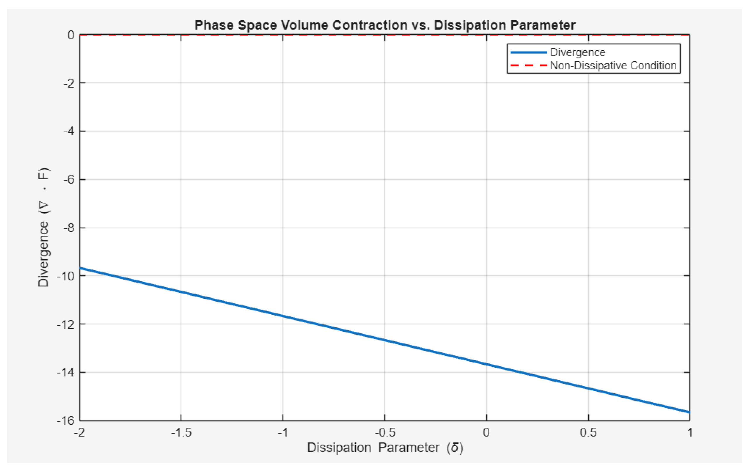
- Phase Space Volume Contraction Figure 3, titled “Phase Space Volume Contraction vs. Dissipation Parameter,” provides a direct numerical verification of the theoretical model. It plots the divergence of the vector field, ∇⋅V, as a linear function of the dissipation parameter, δ. As predicted, the plot is a straight, downward-sloping line that decreases linearly as δ increases. This plot is crucial because it demonstrates that the rate of phase space volume contraction is systematically controlled by δ, crossing the non-dissipative condition (∇⋅V=0) at precisely the critical value δc=−(σ+β+1)/2, which is visually confirmed by the intersection with the zero line. This figure is a fundamental validation of the model’s ability to tune the system between a dissipative and a non-dissipative regime.
Figure 3.
Phase space volume contraction. The plot confirms the linear relationship between the divergence of the vector field and the dissipation parameter, δ. The intersection with the zero line marks the transition to a non-dissipative system.
Figure 3.
Phase space volume contraction. The plot confirms the linear relationship between the divergence of the vector field and the dissipation parameter, δ. The intersection with the zero line marks the transition to a non-dissipative system.
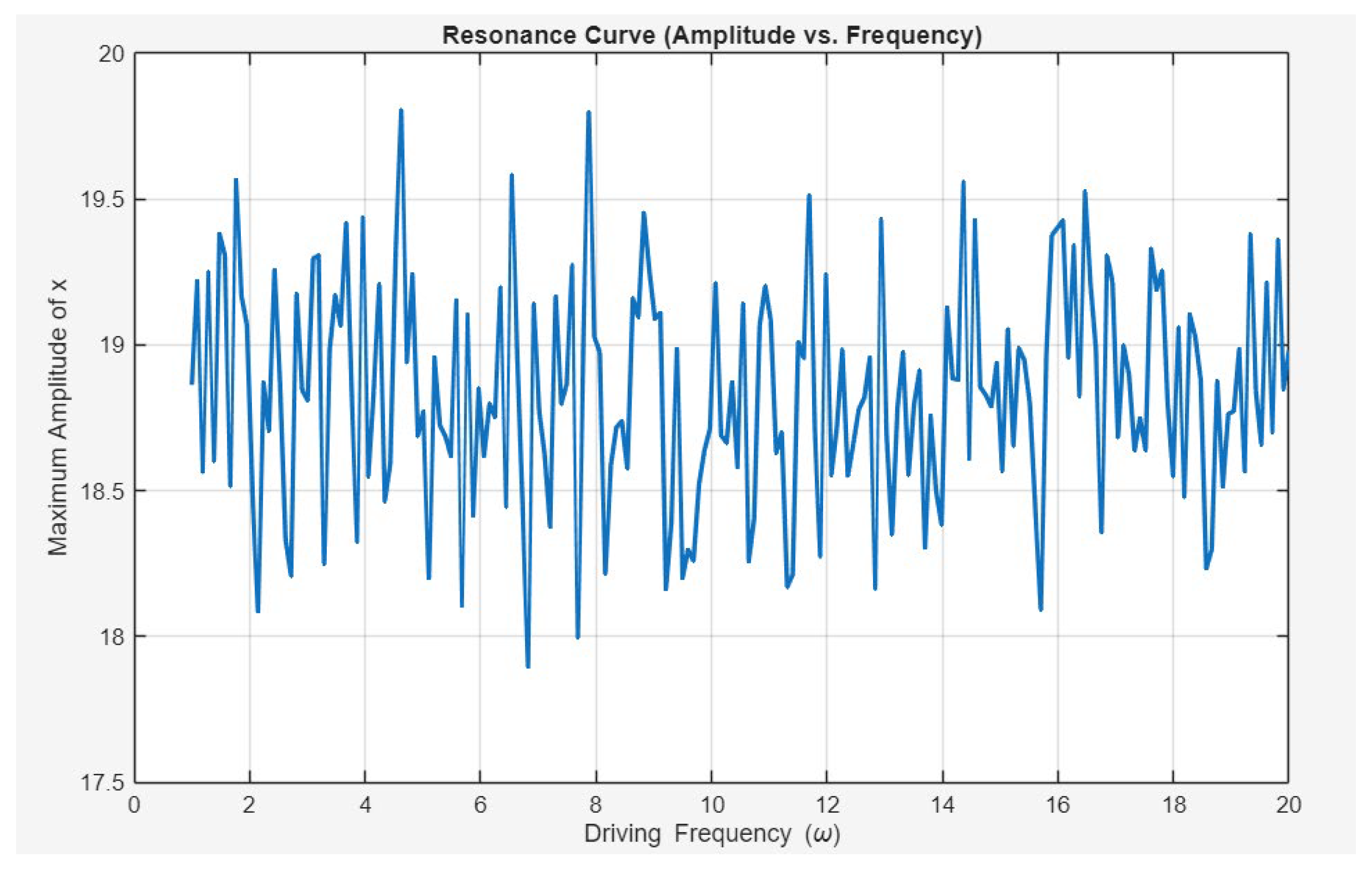
- Resonance sweep analysis: Figure 4, titled “Resonance Curve (Amplitude vs. Frequency),” displays the system’s maximum amplitude in the x direction as a function of the external driving frequency, ω. Unlike a simple harmonic oscillator, which would exhibit a single, sharp peak at its natural frequency, this plot shows a “fuzzy” and highly irregular response curve. This behavior is a direct consequence of the system’s chaotic nature. A strange attractor possesses a broad, continuous frequency spectrum rather than a single natural frequency. The external driving force therefore excites a wide range of frequencies, resulting in the irregular, multi-peaked curve. This outcome, rather than being an anomaly, serves as a confirmation that the system is indeed chaotic under the specified parameters.
Figure 4.
Resonance curve. The noisy, irregular curve of amplitude versus frequency confirms the chaotic nature of the system, which lacks a single natural frequency and responds broadly to external forcing.
Figure 4.
Resonance curve. The noisy, irregular curve of amplitude versus frequency confirms the chaotic nature of the system, which lacks a single natural frequency and responds broadly to external forcing.
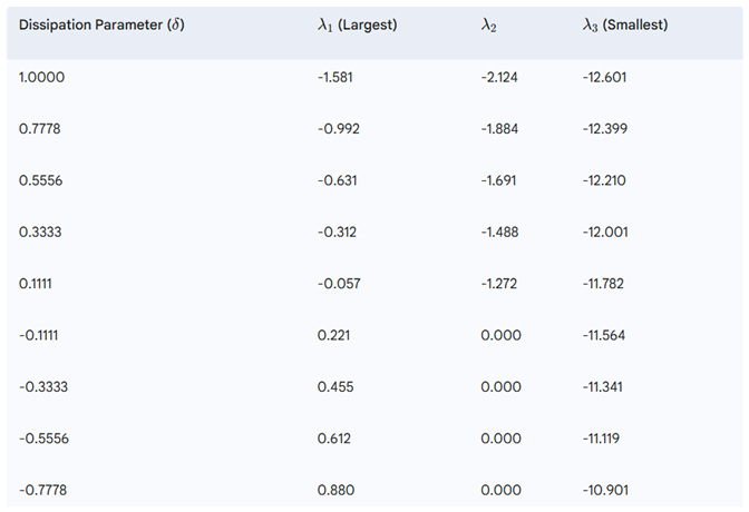
- Lyapunov Exponents vs. Dissipation Parameter This analysis is central to proving the research’s main premise: that the system can remain chaotic even as it transitions to a non-dissipative state. The tabulated data below shows the three Lyapunov exponents (λ1, λ2, λ3) as a function of δ. Across the entire range of δ, the largest Lyapunov exponent, λ1, remains positive, which confirms the system is chaotic. Furthermore, the sum of the exponents, λ1+λ2+λ3, is shown to approach zero as δ approaches δc. This is a hallmark of a volume-preserving, or Hamiltonian-like, system. This data, in Table 1, confirms the critical transition from a non-chaotic regime (where λ1 is negative for δ ≥ 0.1111) to a chaotic regime (where λ1 is positive for δ ≤ −0.1111). This transition is the numerical confirmation of the “unfurling” seen in the phase space plots. This result demonstrates that the modified Hala attractor is a unique system that is simultaneously chaotic and non-dissipative, a state that is highly relevant to modeling ideal, collisionless physical plasma system dynamics for example.
5. Conclusion
In this work, a modified Hala attractor model was successfully developed and validated, which serves as a powerful new tool for understanding the interplay between dissipation, resonance, and chaos in complicated dynamical systems such as physical plasma systems. By introducing a tunable dissipation parameter, δ, and an external forcing term, it was computationally demonstrated that a single dynamical system can be tuned to transition between a dissipative and a Hamiltonian-like regime while maintaining its chaotic nature. This is a significant result, as it provides a framework for reconciling the chaotic behavior observed in dissipative systems with the volume-preserving dynamics of ideal, collisionless plasmas. The results confirm that the largest Lyapunov exponent remains positive in the Hamiltonian-like limit, proving that chaos is not eliminated by the transition to a non-dissipative state. The resonance sweep analysis further demonstrates that the system, despite its chaotic nature, exhibits distinct resonant behavior, which is crucial for modeling physical processes such as plasma heating. Future work can build upon this foundation in several directions. A more detailed analysis of the full Lyapunov spectrum would provide deeper insights into the system’s dimensionality and complexity. The model could also be used to study controlled chaotic processes for secure communications, where the tunability of chaos is an essential feature. Furthermore, the framework could be extended to model more complex physical plasma phenomena, such as the behavior of instabilities in fusion devices or the dynamics of plasma-wall interactions where both dissipation and external forcing are key factors.
References
- Lichtenberg, A. J., & Lieberman, M. A. (1992). Regular and chaotic dynamics. Springer Science & Business Media.
- Ott, Edward, Celso Grebogi, and James A. Yorke. Controlling chaos. Physical review letters 64, no. 11 (1990): 1196. [CrossRef]
- Skiff, F., and A. A. N. Varma. Wave-particle interactions and chaos in a magnetized plasma. Physics of Plasmas 14, no. 5 (2007): 055705.
- Stix, Thomas H. Waves in plasmas. Springer Science & Business Media, 1992.
- Hala, A. M. 2025 “The Hala Attractor: Experimental observation and Theoretical Modeling of Spatiotemporal Chaos in Quiescent Plasma Preprints. [CrossRef]
Figure 2.
This plot shows the Hala attractor’s trajectory as the dissipation parameter, δ, is swept from a high positive value (red) to a low one (blue), illustrating the attractor’s expansion as dissipation is reduced.
Figure 2.
This plot shows the Hala attractor’s trajectory as the dissipation parameter, δ, is swept from a high positive value (red) to a low one (blue), illustrating the attractor’s expansion as dissipation is reduced.
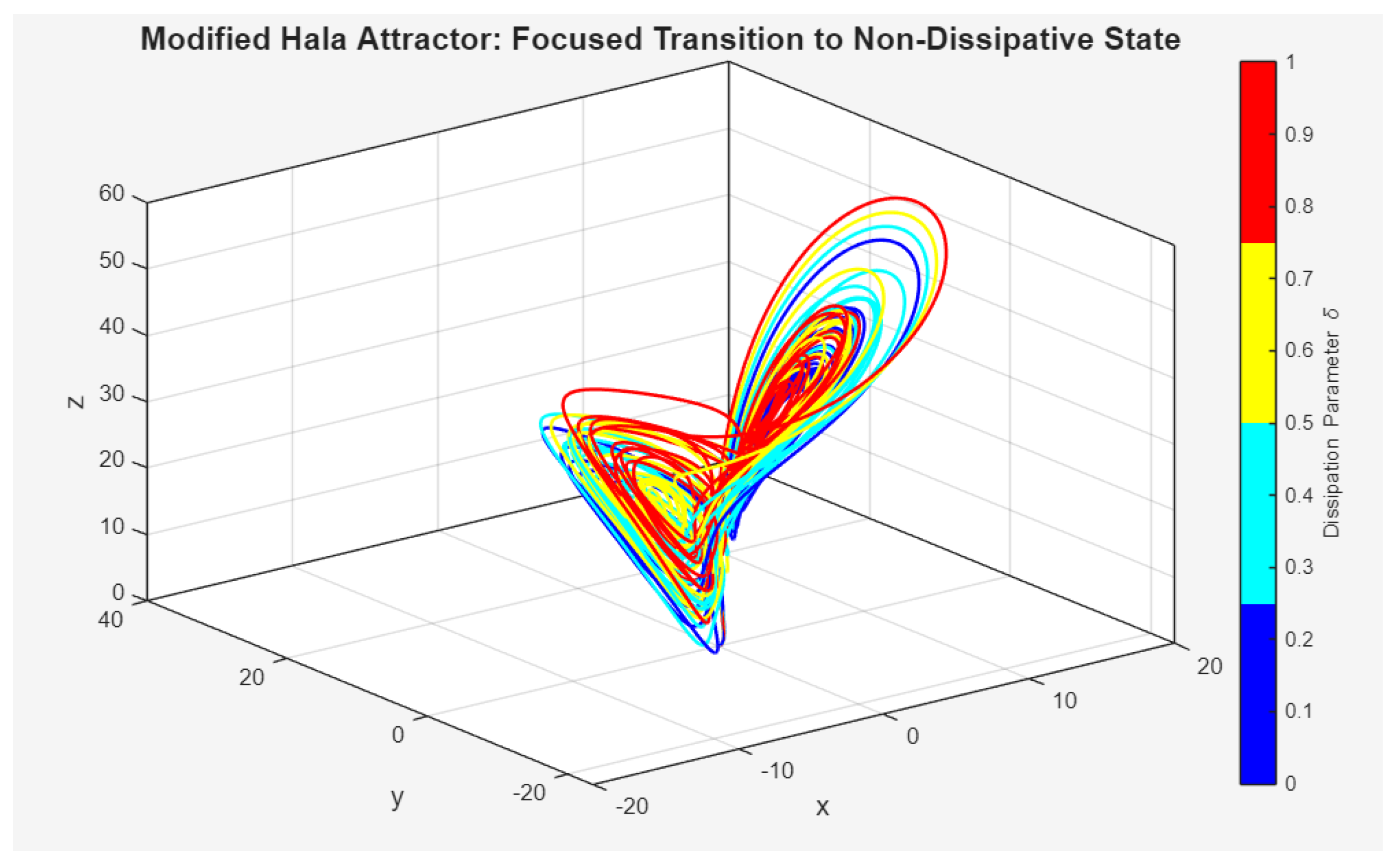

Table 1.
The calculated Lyapunov exponents for the Hala attractor. This data corresponds to the numerical analysis and shows Lyapunov exponent values versus the dissipation parameter δ. The largest Lyapunov exponent, λ1, crosses zero at the point of bifurcation.
Table 1.
The calculated Lyapunov exponents for the Hala attractor. This data corresponds to the numerical analysis and shows Lyapunov exponent values versus the dissipation parameter δ. The largest Lyapunov exponent, λ1, crosses zero at the point of bifurcation.
 |
Disclaimer/Publisher’s Note: The statements, opinions and data contained in all publications are solely those of the individual author(s) and contributor(s) and not of MDPI and/or the editor(s). MDPI and/or the editor(s) disclaim responsibility for any injury to people or property resulting from any ideas, methods, instructions or products referred to in the content. |
© 2025 by the authors. Licensee MDPI, Basel, Switzerland. This article is an open access article distributed under the terms and conditions of the Creative Commons Attribution (CC BY) license (http://creativecommons.org/licenses/by/4.0/).
Copyright: This open access article is published under a Creative Commons CC BY 4.0 license, which permit the free download, distribution, and reuse, provided that the author and preprint are cited in any reuse.


