
Submitted:
15 August 2025
Posted:
15 August 2025
You are already at the latest version
Abstract
Tubulin is one of the major structural proteins that exists either as free forms or as microtubules. These microtubules have unique characteristics, termed as ‘exquisite dynamic behavior’, that is associated with the polymerization and depolymerization of the microtubules or the tubulin units. In cancer cells, the tubulin-mediated dynamicity is lost owing to the elevated expression and functioning of microtubules. These lead to uncontrolled cancer cell proliferation, evading controlled cell cycle checks, survival, and resistance to existing cancer chemotherapy. Considering this, the tubulins/microtubules are validated drug targets in cancer. The agents targeting the microtubules are called microtubule-targeting agents (MTAs). These agents are further subclassified into three groups and act at 7 druggable sites identified so far. However, the majority of inhibitors approved are phytochemicals and are semisynthetic-derived, which are associated with poor pharmacokinetics and toxicities that hamper their clinical use. The rapidly growing cancer cases globally demands rapid drug discovery. One of the rapid and recommended ways for drug discovery is drug repurposing or repositioning. To achieve this, we employed machine learning (ML)-driven, integrated with in silico-based high-throughput virtual screening of 4500 FDA-approved compounds to identify new tubulin inhibitors interacting with the Colchicine Binding Site (CBS) with anticancer potential. The virtual screening workflow was supported by structure-based drug design approaches including three stages of molecular docking, MM-GBSA binding free energy calculations and molecular dynamics (MD) simulations, leading to a refined library of potential tubulin inhibitors. The best hit compounds were tested biochemically to verify tubulin inhibition, as well as tested against a panel of cancer cell lines, whereby Omeprazole and Podofilox demonstrated promising results. The outcomes of this work may lay a solid foundation for further drug development projects, targeting tubulin and cancer via drug repurposing.
Keywords:
machine learning
; drug discovery
; drug repurposing
; structure-based drug design
; virtual Screening
; tubulin polymerization
1. Introduction
Tubulin is one of the major structural proteins that exists either as in free form or as microtubules.[1] Morphologically, tubulin exists in two major isoforms, α- and β-tubulin.[2] These isoforms of tubulin polymerise in a head-to-tail fashion to form protofilaments. The formed protofilaments, when reach thirteen in number, further polymerise to cylindrical structures called ‘microtubules’.[3,4] These microtubules thus formed have a positive and negative end, wherein the positive end exposes the β form of tubulin while the negative end comprises α-tubulin.[5] These microtubules, so formed, have unique characteristics, termed as ‘exquisite dynamic behavior’ that is associated with the polymerization and depolymerization of the microtubules or the tubulin units.[6] This is vital in maintaining the cell shape and assists in the process of cell division, particularly karyokinesis, where it is involved in the formation of the mitotic spindle. Tubulin protein has cytoskeleton and mitotic spindle-forming properties that are essential for cellular transport and division. This dynamic behaviour is catalysed by the guanosine triphosphate (GTP) hydrolysis, followed by the guanosine diphosphate GDP/GTP exchange cycles. The GTP bound to the α-tubulin subunit is referred to as ‘N-site’ while the GTP bound to the β-tubulin is called ‘E-site’.[7] Among these two sites, the N site is stable and does not undergo hydrolysis or the exchange cycle, whereas the E site is unstable and undergoes hydrolysis and exchange with free GDP.[8,9] Thus, considering this, the N-site (GTP bound) promotes the growth of microtubules, and the E-site (GDP bound) does not undergo polymerization. Any hindrance or negative signaling in the N-site (also referred to as the GTP-bound tubulin cap) allows the microtubules to enter the depolymerization phase. The brief illustration of this dynamicity and outcome is reflected in Figure 1.
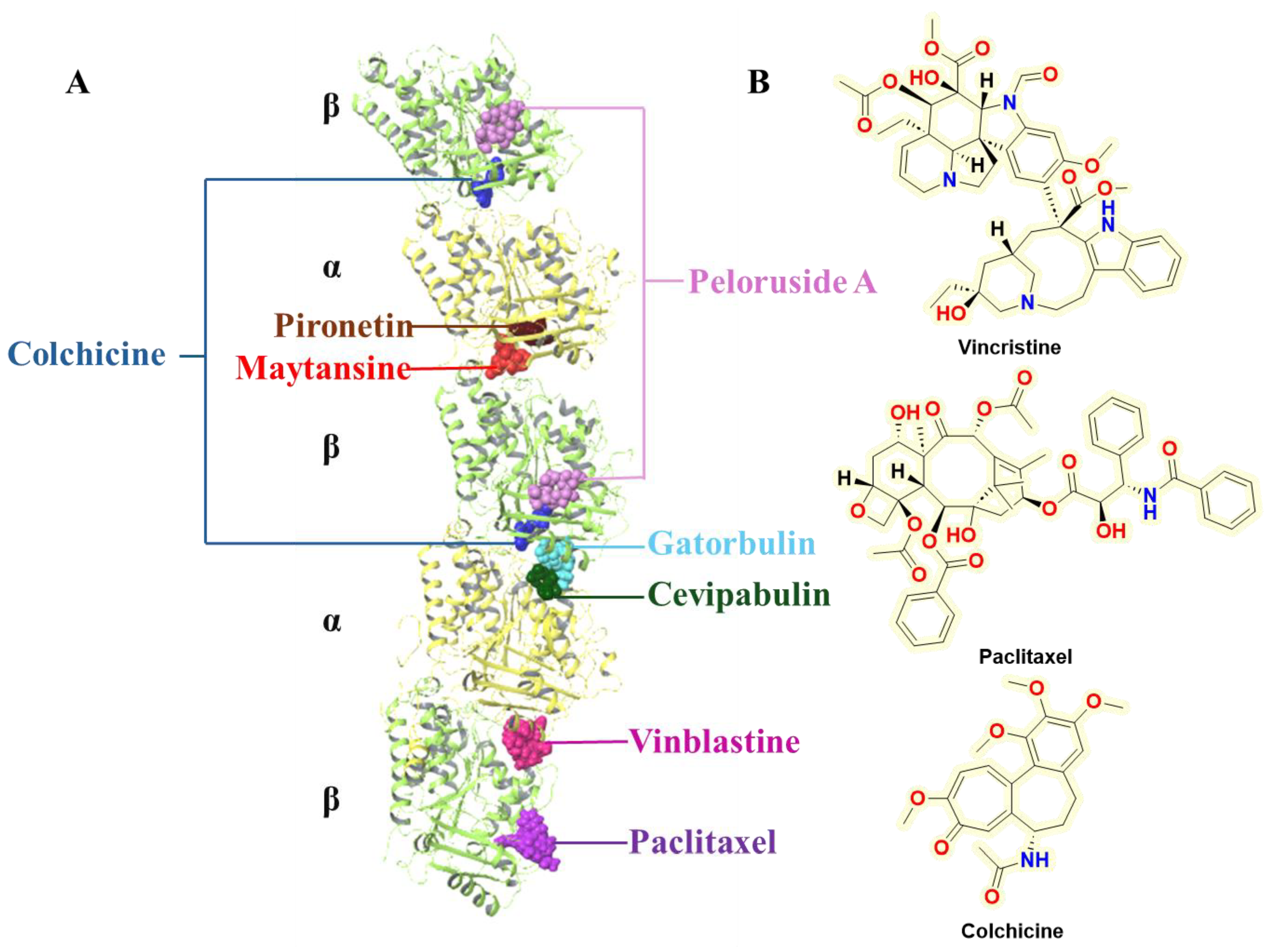
In cancer cells, which are metabolically more active, this dynamicity is lost owing to the elevated expression and functioning of microtubules.[10,11] These lead to uncontrolled cancer cell proliferation, evading controlled cell cycle checks, survival, and resistance to existing cancer chemotherapy.[12] Considering that tubulin and microtubules are considered one of the major anticancer drug targets. To control the unrestrained dynamicity of the microtubules, numerous inhibitor classes for microtubules have been proposed. The agents targeting the microtubules and involved in altering the dynamicity are called microtubule-targeting agents (MTAs). These agents are further subclassified into three groups: (i) microtubule-stabilizing agents (MSAs), which promote polymerization stabilization. MSAs act towards taxanes and laulimalide/peloruside-A binding site.[13] Key inhibitors include Paclitaxel, Docetaxel, Epothilones including Ixabepilone, Patupilone, Laulimalide, and Peloruside; (ii) microtubule-destabilizing agents (MDAs) are associated with the polymerization inhibition and promote depolymerization.[14] MDAs interact with the five distinct binding sites, including the vinca domain, the colchicine domain, the pironetin site, the maytansine site, and the most recently discovered seventh site, known as the gatorbulin-1 site.[5,15] This site represents a dual behavior (MTs destabilizing or tubulin degraders) depending on the compounds binding to it. To exemplify, cevipabulin binds to the vinca site as a microtubule destabilizer and to the seventh site as a tubulin degrader.[16] The key drugs in this category include vinblastine, colchicine, nocodazole, tivantinib, pironetin, maytansine, gatorbulin-1 (GB1), cevipabulin (also known as TTI-237), and (iii) microtubule-targeting degraders (MTGs), which are associated with the microtubule denaturation leading to its degradation.[17] The drugs in this category include withaferin-A,[18] T0070907,[5] 3-(3-phenoxybenzyl)amino-β-carboline(PAC),[5] and cevipabulin, [19]which exhibit tubulin-degrading properties. 2D chemical structures of these inhibitors are presented in Figure 2A.
All these drugs, though have different mechanisms, lead to cancer cell death by causing microtubule abnormalities and affecting the cell cycle. The reported molecules are known to bind to seven distinct druggable sites (Figure 2B) present in microtubules.[5] This includes the major sites: taxane (paclitaxel and docetaxel), vinca (vinca alkaloids such as vincristine and vinblastine), and colchicine binding site (colchicine and combretastatin A-4), and lesser-explored sites that include maytansine, peloruside-A (laulimalide), and gatorbulin site.[20,21] Among these reported sites, the colchicine binding site (CBS) was the first site identified in the tubulin that was explored both for cancer and non-cancer diseases and disorders.[15,22,23] This site is also important because the inhibitors binding to this site have unique mechanisms that inhibit the tubulin assembly. Furthermore, it possesses a deep hydrophobic pocket located at the interface of α- and β-tubulin and making it a favorable druggable site for small molecules binding.[24,25,26] Unlike taxane and vinca sites, CBS inhibitors acts on rapidly dividing cancer cells. The CBS moreover involves unique mechanism of inhibiting polymerization, thus overcoming resistance mechanisms associated with β-tubulin overexpression or drug efflux mediated by the P-glycoprotein. In addition to the anticancer effect, the inhibition of CBS site is also associated with anti-inflammatory and anti-angiogenic properties that further synergizes the anticancer effects.[27,28]
As the majority of inhibitors are phytochemicals or semisynthetic derivatives, they are associated with poor pharmacokinetics and toxicities that hamper their clinical use.[12,16] While the research is ongoing to identify and develop safer and more effective molecules targeting CBS, the rapidly growing cancer cases globally demand rapid drug discovery. Cancer evolves more rapidly owing to drug resistance, inadequate pharmacokinetics, and toxicities of existing chemotherapeutic agents.[4,29] This puts a global burden on the pace of current anticancer discovery and raises a quest for the utmost need for drug discovery and anticancer drug development. One of the rapid and recommended ways for drug discovery is drug repurposing or repositioning.[30] Traditional approaches in developing novel drugs are limited by high cost and time, and have been largely surpassed by designing some efficient computational workflows for drug design, including structure-based drug design (SBDD) and ligand-based drug design (LBDD),[31] considering in silico drug repurposing. The main advantage of the in-silico drug design is to implement the drug discovery research projects to discover new compounds with the potential to be transformed into new therapeutic agents in less time and at a lower cost than the traditional drug discovery approach. There are several significant methods in the in-silico drug design approach, including homology modelling, molecular docking, high-throughput virtual screening, quantitative structure activity relationship (QSAR), 3D pharmacophore mapping, and molecular dynamics (MD) simulations [15,32]. Moreover, recent integration of artificial intelligence (AI)[33] and machine learning (ML) [34] in these workflows have significantly accelerated the drug discovery pipeline. By leveraging vast commercially available huge chemical libraries and screening large number of molecules virtually, AI and ML allow exploration of chemical space at a scale and speed, outperforming traditional experimental approaches.[35]
To achieve plausible CBS inhibitors with anticancer potential, we performed an ML-driven computational drug repurposing study, using 4500 USFDA-approved drugs.[36] The ML workflow was combined with the computer-assisted drug design (CADD) strategy to identify promising tubulin inhibitors with anticancer activities. Structure-based drug design refinements such as molecular docking, MM-GBSA binding free energy calculations, and molecular dynamics (MD) simulations allowed us to identify three promising hit molecules, i.e., podofilox, omeprazole, and sulfadoxine, which inhibit the CBS site of tubulin and could be further developed as anticancer agents. The identified hits were biologically corroborated by performing a tubulin polymerization assay, understanding the cytoskeletal disruption, and their anticancer potential was established in a panel of cancer cell lines, and the impact on cell cycle analysis and apoptosis was assessed.
2. Materials and Methods
2.1. Machine Learning Workflow
2.1.1. Data Acquisition and Filtration
A total of 907 tubulin inhibitors with the reported IC50 values in the range of 0.25 to 400 μM were retrieved from the ChEMBL35 database [37], ID = CHEMBL2094134 for tubulin https://www.ebi.ac.uk/chembl/explore/target/CHEMBL2094134. The 907 compounds’ dataset was filtered to 501 compounds, based on meeting two criteria: (a) all assays are binding assays, (b) all compounds have undergone similar assay methodology. i.e., the inhibition of bovine brain tubulin polymerization by spectrophotometry. The 501 compounds were further finetuned to 379 compounds after implementing ‘Ligand Preparation’ using the LigPrep [38] module of Maestro, Schrodinger [39] (discussed below). In addition to generating a low-energy optimal 3D structure from SMILES (as discussed in the ‘Ligand preparation section below), the ML dataset involved the removal of duplicates and salts. Based on the distribution of IC50 values associated with the compound dataset, two thresholds for classifying compounds were defined. Specifically, compounds with IC50 ≤ 3.0 μM (pIC50 ≥ 5.5) were labelled as active, whereas compounds with IC50 ≥ 12 μM (pIC50 ≤ 4.9) were labelled as inactive. The compounds in the mid-range (often called the gray range in ML) of IC50 values, i.e., from 3.0 to 12 μM (4.9 to 5.5 pIC50), were removed from the dataset so that robust ML models can be developed. Eventually, a total of 289 compounds were defined as the internal ML dataset comprising 161 active and 118 inactive compounds.
2.1.2. Decoys Generation
The balance of data sets is critical for developing a solid predictive model. The performance of the ML model is highly influenced by data imbalance between classes. To balance the data set of 289 compounds, 157 decoy compounds were generated by computing their molecular properties based on the reported tubulin inhibitors using the DUDE online database [40] (http://dude.docking.org/).
2.1.3. Model Development and Evaluation
The dataset containing 279 known tubulin inhibitors with experimental pIC50 values, categorized into actives (pIC₅₀ ≥ 5.5) and inactives (pIC₅₀ ≤ 4.9). An independent external set of 157 decoy compounds (pIC₅₀ ≤ 4.9) was used exclusively for external validation. Model generation was performed using the AutoQSAR[41] module of Maestro, Schrödinger 2024-2 version.[39] By default, all available descriptor classes were included in model building, comprising binary fingerprints such as radial, linear, dendritic, and molprint2D, and numerical descriptors including topographical, physicochemical, and ligand-based filter (Ligfilter) properties. The internal dataset of 279 inhibitors was randomly split into a training set (75%) and an internal test set (25%). Training data were used to construct Bayesian classification (Bayes) and recursive partitioning (RP) models, applying AutoQSAR’s internal k-fold cross-validation for hyperparameter optimization. Internal test set performance was assessed using statistical parameters including coefficient of determination (R²), cross-validated coefficient (Q²), root-mean-square error (RMSE), and Matthews correlation coefficient (MCC). Final model performance was further evaluated against the external decoy set to assess predictive generalization. The best-performing model was subsequently employed for virtual screening of the USFDA chemical library to identify novel tubulin inhibitor candidates.
2.2. Protein Preparation and Optimization
The X-ray crystal structure of the target tubulin protein in complex with the bound inhibitor, G8K ([2-(1H-indol-4-yl)-1H-imidazol-4-yl](3,4,5-trimethoxyphenyl) methanone) (PDB ID: 6O5M)[42] was retrieved from the Protein Data Bank [43]. The protein preparation wizard [44] , as implemented in Maestro, Schrödinger [39], was used to prepare the co-crystallized structure. The Prime module of Schrödinger was used to add/optimize H-bonds, missing side chain atoms and loops to the X-ray structure, followed by assigning protonation states and generating tautomeric forms for Asp, Glu, Arg, Lys and His at pH 7.0 ± 2.0. The PROPKA module of Schrödinger was used for H-bond refinement of the protein structure at pH 7.0, which involved addressing any overlapping hydrogen atoms. Water molecules with fewer than two hydrogen bonds to non-waters were deleted. With the purpose of fixing molecular overlaps and strains, geometry refinements of the protein structure was performed using the OPLS4 force field in a restrained minimizations until the average root mean square deviation (RMSD) of the protein heavy atoms converges to 0.3 Å.
2.3. Ligand Preparation
The co-crystallized inhibitor G8K and the selected database comprising 4500 drug molecules were prepared using the LigPrep module as implemented in Maestro, Schrödinger. The OPLS4 force field was employed to perform energy minimization on the ligands. Epik, a tool for predicting pKa values (acid dissociation constants), was employed to assign possible tautomeric and ionization states at pH 7.00 ± 2.00.
2.4. Receptor Grid Generation
The prepared protein structure of tubulin in complex with G8K (PDB ID: 6O5M) was used for generating a receptor grid for the docking of 4500 compounds into the colchicine binding site (CBS) of tubulin. A cubic receptor grid was generated with respect to the centroid of the co-crystallized ligand G8K in the substrate binding site, with a side length of 20 Å [45,46]. No constraints were applied in the generation of the receptor grid. The default parameters of the 1.0 scaling factor for van der Waals radius of nonpolar parts of the receptor atoms and 0.25 partial charge cutoff were used.
2.5. Molecular Docking
Docking experiments were performed by using the Glide [45,46] module of Schrödinger [39], employing the 4500 FDA-approved compounds. Docking was carried out under default settings, using the high-throughput virtual screening (HTVS) mode, standard precision (SP) mode, and the extra precision (XP) mode, allowing flexible ligand sampling, also involving nitrogen inversions and ring conformations of the ligands. The default parameters of the 0.80 scaling factor for van der Waals radii of nonpolar ligand atoms and 0.15 partial charge cutoff were used. We performed post-docking minimization by including 5 poses per ligand during HTVS and SP docking, and 10 poses per ligand during XP docking. During XP docking, the threshold for rejecting minimized poses was set to 0.50 kcal/mol. No constraints were applied to the ligand docking. The Epik state penalties were added to the docking score, and the default Glide scoring function was used to select the top-ranked docking pose for each ligand from each docking protocol.
2.6. Binding Free Energy Calculations
Molecular mechanics with generalized Born and surface area solvation (MM-GBSA) is a method to predict the binding free energy of a ligand bound to a protein, and it can quantitatively characterize the binding details of ligand–receptor systems [47]. MM-GBSA has been widely used in protein–ligand binding, protein–protein interactions, and protein folding. The Prime module in Schrödinger suite 2024-2[39] was used to compute MM-GBSA free energy of binding (ΔG Bind) for the crystallographic and docking poses, with respect to the tubulin protein, using the following equation:
where EComplex, ELigand, and EReceptor represent the energies calculated in the Prime MMGBSA module for the optimized complex (complex), optimized free ligand (ligand), and optimized free receptor (receptor), respectively. The OPLS4 force field[48,49] and VSGB (Variable Dielectric Surface Generalized Born) solvation model were used in the binding free energies calculations, featuring minimization of protein–ligand complexes as the sampling method. The binding free energies (ΔG Bind) and the Coulomb energy (ΔG Coulomb) of each ligand were highlighted in this study.
ΔG Bind = EComplex – ELigand – EReceptor
2.7. Molecular Dynamics Simulations and Clustering
Being an imperative step in any computational modeling project, classical MD simulations were performed using the Desmond program [50,51] in Schrödinger suite 2024-2 [39], starting from the crystallographic pose of the existing inhibitor (G8K) or the top-ranked docking poses of hit compounds in the colchicine binding site of the tubulin. In the system builder panel as implemented in Maestro, Schrödinger, each protein–ligand complex was solvated in the transferable interatomic potential with three-point water model (TIP3P) [52] with an orthorhombic box solvent model with periodic boundary conditions, placed in such a way that the walls were at a minimum 10 Å distance from every atom in the system. Appropriate Na+ ions were added to neutralize the overall charge of each system. A salt concentration of 0.15 M NaCl was added to the simulation box to create physiological conditions. The default Desmond protocol in the NPT ensemble was used for minimization and relaxation of each system [53,54,55]. The OPLS4 force field was applied during all simulations. Each simulation was run for a total of 200 ns with a recording interval of 200 ps. The approximate number of frames and energy were set to 1000 and 20, respectively. The temperature and pressure of the system were kept constant at 300 K and 1.01325 bar atmospheric pressure, respectively.
After the completion of MD simulations, the simulation trajectories were analyzed for root-mean-square deviations (RMSD), protein–ligand interactions, and root-mean-square fluctuations (RMSF) of both protein and ligands, using the simulation interaction diagram module of the Schrödinger suite. Using the “Desmond Trajectory Clustering” module,[51] the obtained trajectories were clustered, setting up a frequency value of 10 (every 10th ns) and up to a maximum of 2 clusters. With regard to the MD simulations of co-crystallized complex, the obtained cluster resembling the crystallographic pose was used as a representative structure, while with respect to the MD simulations of docked complexes (hit molecules), the most populated cluster was used as a representative structure.
2.8. Biological Investigations
2.8.1. Tubulin Polymerisation Assay
The tubulin polymerization assay was performed using the tubulin polymerization HTS assay kit (BK004P) purchased from Cytoskeleton Inc. The tubulin, as per the kit specification, is derived from Porcine with >97% purity. The assay relies on the principle that under optimal reaction conditions and temperature, the tubulin polymerizes into microtubules, which leads to either a change in turbidity (in our case) or fluorescence that is further measured spectrophotometrically. The increase in the turbidity is associated with the polymerization, whereas the decrease indicates the depolymerization. We performed the assay according to the manufacturer’s protocol with some modifications. In brief, all the supplied materials in the kit were diluted as per the protocol and kept on ice during the experiment. G-PEM buffer was prepared by warming 990 µL of General Tubulin Buffer and supplemented with 10 µL 100 mM GTP (80 mM PIPES, pH 6.9, 2 mM MgCl₂, 0.5 mM EGTA, 1 mM GTP). The reaction was initiated by adding 10 µL of 10× compound per well (Final concentration: 5 µM) and was incubated for 2 min at 37 °C. To this, 100 µL of 4 mg/mL tubulin (from 4 °C) was added to the wells. Upon addition, we immediately started the kinetic reaction. The hits in comparison to the supplied paclitaxel were tested at a concentration of 5 µM in kinetic mode, run at 37 ℃ for 60 minutes in the FlexStation 3 Multi-Mode Microplate Reader at absorbance set to 340 nm. In addition, the percentage inhibition of microtubule formation at each concentration was also calculated at the intervention concentrations of 5 µM.
2.8.2. Cell Culture and Cytotoxicity MeasurementsCell Growth and Maintenance
The cancer cells (SK-MEL-28, A549, PC-3, MCF-7, MDAMB-231, HCT-116) were procured from the Institute of Cancer Therapeutics, University of Bradford, in-house repository. The cells were grown under sterile conditions using RPMI media supplemented with 5% fetal bovine serum (FBS) and 5% glutamine in the bio-incubator with 5% CO2 concentration and 75% RH at 37 ℃. Upon attaining 80% confluency, the present media and cells were washed once with 1X PBS and supplemented with trypsin (5%) to T-75 flasks and incubated for 5 minutes for trypsinization. The trypsinized cells were split at this moment or were grown in either Sarstedt 96 or 6-well plates for performing the required experiments. These were further grown as per the mentioned conditions and periodically trypsinized, or a media change was done to maintain their morphology and health.
Resazurin Assay
Resazurin assay was conducted to evaluate the metabolic activity (live or dead) of the cancer cells upon the treatment with the leads. The assay relies on the ability of living cells to reduce the resazurin dye (non-fluorescent) into resorufin (fluorescent) by the catalytic activity of the mitochondrial reductase. The formation of resorufin is quantified spectrophotometrically, and an account of live cells left upon treatment is made with the untreated cells. In brief, we seeded approximately 8000 cells in each well of a 96-well plate using 200 µL complete media per well. The cells were grown under standard conditions overnight, and upon confluency, treatment was made with the identified hits at concentrations of 1, 5, and 25 µM in comparison to the positive controls, paclitaxel and colchicine, employed during the assay. The cells with the treatment of interventions and positive controls were incubated for 48h before analysing them using the resazurin assay. The media from each well was completely removed and was replenished with the resazurin dye (prepared using a 2 mg/mL solution of resazurin with 1X PBS). This was kept in the dark and diluted 1:10 with the media before use. Each well was replenished with 200 µL resazurin solution, and the plate was kept in an incubator for 4-5 h. After the stipulated time, the plates were removed, and 100 µL solution from each plate was aspirated into a black plate with a clear bottom. These plates were read spectrophotometrically read at fluorescence of λEx of 545 nm and λEm of 595 nm. The values obtained were further normalised with the untreated control, and the percentage inhibition at each concentration was calculated, which was further used to calculate the half maximal inhibitory concentration (IC50) of the identified leads with respect to the positive control.
Confocal Analysis to Quantify the Tubulin Disruption
We indirectly analysed the tubulin disruption by studying the F-actin-stained cytoskeletal network using CellMask™ Green Actin Tracking Stain from ThermoFisher (#A57243). This dye is sensitive and indicates a downstream readout of the microtubule perturbation. Changes in F-actin architecture are measured to foresee how the microtubule disruption rewires the cytoskeletal system in the cells where microtubules and actin are integral parts. The assay was performed in accordance with the manufacturer’s protocol, whereby the HCT-116 cells were treated (on coverslip) with the interventions at a 5 µM concentration for 24 hours. After the stipulated durations, the media was removed and the coverslips with cells were washed with IX PBS, and were stained with F-actin dye and DAPI, fixed using mounting media, and analysed using a fluorescence microscope using green and blue channels. A brief overview of the undertaken work is represented in Scheme 1.
3. Results and Discussion
3.1. Machine Learning Model Development
The AutoQSAR-based machine learning workflow[41] in Maestro, Schrödinger[39] was employed to develop predictive classification models for tubulin inhibitors. The curated dataset consisted of 279 compounds with experimentally determined pIC₅₀ values, categorized as actives (pIC₅₀ ≥ 5.5) and inactives (pIC₅₀ ≤ 4.9). An independent external validation set comprising 157 decoy compounds (pIC₅₀ ≤ 4.9) was reserved exclusively for final model testing. By default, AutoQSAR utilizes a comprehensive set of descriptors, including binary fingerprints (radial, linear, dendritic, and molprint2D) as well as numerical descriptors, including topographical, physicochemical, and Ligfilter properties.
Multiple models were generated using different algorithm–descriptor combinations. Among these, Bayesian classification (Bayes) and Recursive Partitioning (RP) models consistently achieved top ranks. In particular, Bayes models employing dendritic and linear fingerprints (i.e., bayes_dendritic_1 with a model score of 0.9389, and bayes_linear_20 with a 0.9337 model score) displayed the highest internal validation scores, with strong R² and Q² values, low RMSE, and balanced classification metrics, as mentioned in Table 1. RP models such as rp_30 and rp_41 also performed competitively, demonstrating robust predictive ability across the descriptor set, showing model scores of 0.9158 and 0.9133, respectively.
The model score is a composite metric that combines multiple measures of model quality into a single value between 0 and 1, facilitating the direct comparison of models built using different descriptor sets and algorithms. For classification tasks, the score integrates internal cross-validated accuracy, area under the ROC curve (AUC), enrichment factors, and class-specific error rates, with greater weight given to predictive power and robustness across validation folds. For regression tasks, the score combines the coefficient of determination (R²), cross-validated coefficient (Q²), root-mean-square error (RMSE), and error consistency. Each metric is normalized and weighted before aggregation, ensuring that the final model score reflects both predictive accuracy and stability rather than a single performance statistic. The performance of the best individual ML model, each from Bayes classification and recursive partitioning is enlisted in Table 2 and Table 3, respectively, as well as discussed below.
- Bayesian classification (Bayes)
Bayesian classification is a probabilistic approach grounded in Bayes’ theorem, estimating the posterior probability of class membership given the observed descriptors. AutoQSAR’s Bayes implementation assumes conditional independence among descriptors, which allows efficient handling of high-dimensional feature spaces. In this study, Bayes models integrated both structural fingerprints and numerical descriptors, facilitating the capture of chemical substructure patterns along with the physicochemical properties. The algorithm outputs a probability score for each class (active or inactive), with final classification determined by the higher posterior probability. The robustness of this method with respect to diverse data and the ability to generalize from limited samples make it particularly well-suited for virtual screening tasks involving structurally diverse datasets.
- Recursive partitioning (RP)
Recursive Partitioning is a decision-tree-based algorithm that sequentially divides the dataset into progressively purer subsets according to descriptor thresholds that maximize class separation. Each split is determined by the descriptor value that generates a significant improvement in classification purity, and this process continues until stopping criteria are met. The resulting model can be visualized as a hierarchy of decision rules, making RP inherently interpretable. Its capacity to handle complex, non-linear interactions among descriptors is advantageous for modeling structure – activity relationships in datasets where multiple features collectively influence biological activity.
Internal evaluation was performed using a stratified 75:25 train–test split of the inhibitor dataset, with AutoQSAR applying k-fold cross-validation to the training set for hyperparameter tuning. The internal test results indicated strong generalization within the chemical space represented in the training data, with no signs of overfitting. External validation against the 157 decoy compounds demonstrated high specificity, indicating the models’ ability to accurately recognize inactive compounds and minimize false positives—an essential criterion for virtual screening workflows.
Based on combined internal and external validation metrics, we adapted a consensus strategy for predicting the hit molecules, binding at the CBS of the tubulin, further showing tubulin inhibitor and anticancer activities. Consensus model resulting from the top 10 ML models discussed above was used to screen FDA-approved library of 4500 compounds.
3.2. Molecular Docking
After the ML model development and validation, a consensus strategy was used to consider all the top 10 models and identify new tubulin inhibitors. A chemical library comprising 4500 USFDA approved drugs were predicted through the consensus ML model approach, to identify new compounds. Out of the 4500 FDA approved compounds, X compounds predicted to be ‘active’ against tubulin protein, based on possessing similar structural and molecular properties to that of existing tubulin inhibitors, used in ML training. Before performing structure-based virtual screening operation, we first retrieved and interrogated the X-ray structure of tubulin protein bound to a nanomolar potent inhibitor G8K (PDB code: 6O5M) (Figure 3). The binding mode of the co-crystallized ligand G8K (Figure 4) indicates that it forms water bridge/salt bridge interactions with the Arg 198, Lys 350, i.e., positively charged residues, followed by carbonyl oxygen interactions with Asn112 and Ser132, forming the H-bond. His 114 was also found to participate in an H-bond with the Aza group in the co-crystallised ligand. The aromatic ring systems were found to stabilise the molecule via π–π stacking with Phe169 and Tyr203. Additional interaction with Thr179 and Asn347 in the colchicine binding site highlighted G8K is maintaining interactions with both Further, oxygen and hydrogen atoms of water molecule forms hydrogen bond interactions with the amine hydrogen of the Cys239 and carbonyl oxygen of Gly235 helping towards the binding of G8K with the chain B. Thereby, four amino acid residues Thr179, Asn347, Cys239, and Gly235 contribute substantially towards the ligand interaction within the substrate binding site.
After studying the interactions and the binding mode of the co-crystallized inhibitor G8K at the tubulin binding site, the next step was to select and validate the docking program for our structure-based virtual screening study. The validation of docking was done by redocking the co-crystallised ligand within the same binding site (CBS) of tubulin, As shown in Figure 5, the Glide SP docking poses results in a perfect superposition to that of the co-crystallized pose, possessing an RMSD of 1.18 Å, confirming the reliability of our docking method to be used in the next steps.
As illustrated in the virtual screening workflow diagram in Figure 6, ~1800 compounds were subjected to three stages of docking using the Glide program of Schrödinger: (a) Glide HTVS, (b) Glide SP, and (c) Glide SP to refine the virtual screening workflow and prioritize promising compounds. Glide HTVS docking mode allowed prioritization of 698 compounds among 1800 compounds, possessing docking scores of 9.0 kcal/mol and above. Similarly, the 698 filtered compounds were further docked through the Glide SP docking mode, leading to 350 compounds with docking scores of 9.0 kcal/mol and above. The last stage of docking protocol involved the use of Glide XP mode, which facilitated the refinement of the best 38 compounds showing docking scores of 8.0 kcal/mol and above.
In general, the Glide Score provides an empirical and approximate scoring function, irrespective of providing any information on the actual free energy change. Owing to this, the docking scores often fail to portray the full complexity of molecular interactions. To overcome this, we additionally performed the molecular mechanics (MMGBSA) to calculate the ΔG_bind and ΔG_coulomb, which indicate the estimation of the binding free energy and the accompanying electrostatic interactions between the ligand and the target protein. These parameters provide much more accuracy and full complexity of molecular interactions of the ligand within the binding site. Together, these thermodynamic parameters portray much realistic and refined predictions and provide a true estimation of binding affinity. The Glide XP docking scores of the most promising compounds along with their binding energetics illustrated in Table 4, also compared with the reference co-crystallized inhibitor G8K.
The said analysis revealed that Arformoterol, though it had an excellent docking score, had a poor ΔG_bind, suggestive of a potential outlier. Coming to the potent molecules, Omeprazole exhibited a strong binding (-64.16 kcal/mol), and a moderate electrostatic potential (-58.31 kcal/mol) along with a moderate Glide Score. Podofilox was found to be a perfect solid all-rounder, portraying optimal docking and binding scores of -9.908 kcal/mol and -38.61 kcal/mol, respectively. Thus, based on analysis, we selected podofilox, omeprazole, and sulfadoxine for our further analysis.
Initially, we analyzed the binding pattern of the selected compounds with the CBS. We analysed the podofilox binding pattern, the analysis revealed (Figure 7) that the compound engages the CBS site primarily via the hydrogen bonding with Thr179 (A179). The water molecule present was further found to stabilise the interaction via the hydration network mediated with the involvement of Gly235, Val236, Thr237, and Ile368. Hydrogen bonds between the hydrogen atom of the water molecule and the oxygens of the trimethoxyphenyl group of podofilox help its binding with the water molecule. Further, oxygen and hydrogen atoms of the water molecule form hydrogen bond interactions with the amine hydrogen of Cys239 and the carbonyl oxygen of Gly235, helping towards the binding of podofilox with chain B. Additionally, the hydrophobic enclosure made by amino acid residues, primarily Leu253, Ala248, and Ile316, was also found to be important in stabilising the interaction. The negatively charged Asp249 was also found to provide podofilox optimal electrostatic binding (ΔG_coloumb). Podofilox was shown to portray its binding within the CBS cavity via the extensive water network, hydrophobic, and hydrogen bonding interactions.
Next, we analysed the binding pattern of Omeprazole. The analysis revealed (Figure 8) shows one interaction with the hydroxy group of Thr179 with the protonated nitrogen (N⁺H) of omeprazole. The omeprazole is further found to be stabilised by the hydrophobic amino acid residues such as Val181 (A181), Ala180 (A180), Leu253 (B253) and hydrophilic interaction mediated by the polar residues such as Thr312 (B312), Asn347 (B347) and Asn348 (B348), offering stabilization via the dipole-diploe interactions and hydrogen bonding mediated by the water molecule. In addition to this, charged residues Lys350 and Asp249 further contributed to the electrostatic stabilization. although no direct salt bridges are depicted. Furthermore, aromatic amino acid residues (Phe367 and Phe404) hover the binding cavity, raising the possibility of π-π interactions.
We analyzed the binding pattern of sulfadoxine. The analysis revealed (Figure 9) multiple hydrogen bonds, notably with Asn347, Gly235, and Cys239. Additionally, the electrostatic stability was provided by the Asp249 (B:249) and Lys252 and Lys350 based charged residues. Along with this, a water-mediated hydrogen bond was also found to stabilise the ligand in the CBS. The hydrogen bond between the hydrogen atom of the water molecule and the oxygen of the trimethoxyphenyl group of sulfadoxine helps its binding with the water molecule. Further, oxygen and hydrogen atoms of the water molecule form hydrogen bond interactions with the amine hydrogen of Cys239 and the carbonyl oxygen of Gly235, which also helped towards the binding of sulfadoxine with the chain B. Thereby, three amino acid residues, Asn347, Gly235, and Cys239, contribute significantly towards the ligand interaction within the substrate binding site.
Lastly, the suggested binding mode of the docked compound trimethoprim from the docking studies (Figure 10) shows THR179 (T179) is associated with the formation of a hydrogen bond with TMP water-mediated interaction and another interaction with Thr179 in the colchicine binding site. This allows trimethoprim to maintain interactions with both chain A and chain B of the tubulin heterodimer, thus allowing it a strong binding affinity towards the CBS embedded at the interface of both chains. One other water-mediated interaction was observed by the docking studies in which a water molecule exists as an intermediate, helping towards the binding of trimethoprim with the Gly235 and Cys239 of chain B. The Cys239 contributed to the hydrophobic interactions and was involved in stabilisation via van der Waals forces, while Gly235 formed another bond with the TMP. Thus, three amino acid residues Thr179, Gly235, and Cys239 contribute significantly towards the ligand interaction within the substrate binding site. Besides the hydrogen bonds, hydrophobic enclosure formed via Ala248, Leu 253, and Ile368, and aromatic stabilisation via π-π stacking also played a major role. In a nutshell, the conformation pattern of TMP revealed that it sits deeply embedded in CBS, stabilized primarily by the polar and hydrogen bonding interactions.
3.3. Molecular Dynamics (MD) Simulations
From the cumulative molecular docking and MMGBSA analysis, we concluded podofilox, omeprazole, and sulfadoxine to be the best possible hits. However, the molecular docking analysis assumes the protein to be in a rigid state, undergoing no conformation changes, while the molecular mechanics studies provide an idea of an approximate estimation of the binding energy, which, however, does not take into account the excess water and or solvent residues in the binding site. To overcome this research gap, molecular dynamics (MD) simulations are recommended, which take into account the stability of protein–ligand complex over time when both are in perturbations and have constant fluctuation in the conformations. The MD poses thus assist in confirming whether the binding pose is stable over the simulation period or the binding pose revealed through the docking study was unrealistic, and if there was a transitory protein-ligand binding. To study this, we performed the MD simulations of 200 ns on the top hit identified ligands from the pool.
- MD analysis of the co-crystallised inhibitor G8K
To analyse the conformational dynamicity of the receptor and ligand, the co-crystallized inhibitor, and the docked compounds podofilox, omeprazole, and sulfadoxine were subjected to 200 ns MD simulations, starting from their initial co-crystallized/Glide XP docking poses. During the simulation trajectory, the deviation of the protein and ligand atoms from their initial crystallographic poses is illustrated by the Root Mean Square Deviation (RMSD) and it was calculated for the α-carbons of protein and the ligand heavy atoms throughout the simulation. RMSD plot (Figure 11) demonstrates that the co-crystallized inhibitor and the protein exhibit stability over the course of the simulation. The co-crystallised inhibitor, G8K is maintaining an average RMSD of 1.31 Å during the simulation in the tubulin binding site. The suggested binding mode of the G8K from the docking studies represents one hydrogen-bonded protein-ligand interaction mediated by a water molecule and other interactions with Thr179 (Chain A) and Asn347 (Chain B) in the colchicine binding site. Moreover, it was revealed by MD studies that H-bond interactions with the Thr179 (Chain A), Cys239 (Chain B) and Asn347 (Chain B) was maintained during 96.1%, 17.7% and 77.7% of the simulation time. Furthermore, MD studies demonstrated the presence of an additional H-bond interaction between G8K and Asp249 (Chain B). Although this interaction was not visible in the crystallographic binding pose, yet it was observed during 82.4% of the simulation time.
- MD analysis of Podofilox
The suggested binding mode of the compound podofilox from the docking studies shows one hydrogen-bonded protein-ligand interaction mediated by a water molecule and another interaction with Thr179 (Chain A) in the colchicine binding site. Moreover, it was revealed by MD studies that H-bond interactions with the Thr179 (Chain A) and Cys239 (Chain B) was maintained during 42.3% and 56.4% of the simulation time. Furthermore, MD studies demonstrated the presence of an additional H-bond interaction between the docked compound podofilox and amine hydrogen of Asp249 (Chain B). Although this interaction was not seen in the crystallographic binding pose, yet it was observed during 96.5% of the simulation time. Additionally, we observed that in the crystallographic pose, podofilox interacts with Cys239 (Chain B) by forming hydrogen bond with the amine hydrogen of Cys239 (Chain B) while it interacts with the Cys239 (Chain B) by forming hydrogen bond with the thiol hydrogen as revealed by MD studies. RMSD plot (Figure 12) demonstrates that podofilox and the protein exhibit stability over the course of the simulation, but some fluctuations were observed in between 20-23 ns and 125-150 ns indicating that the podofilox is undergoing some major conformational changes and becoming more flexible in the CBS. Thr179 (Chain A), Cys239 (Chain B) and Asp249 (Chain B) are the common amino acid residues forming H-bond interactions with both co-crystallized inhibitor and podofilox. With podofilox, Thr179 (Chain A) was observed maintaining a low percentage of 42.3% as compared to the co-crystallized inhibitor maintaining this interaction during 96.1% of the simulation time. Furthermore, the H-bond interactions between podofilox and amino acid residues, Cys239 (Chain B) and Asp249 (Chain B) was observed maintaining a high percentage of 56.4% and 96.5% as compared to the co-crystallized inhibitor maintaining this interaction during 17.7% and 82.4% of the simulation time.
- MD analysis of Omeprazole
The suggested binding mode of the compound omeprazole from the docking studies shows one interaction with Thr179 (Chain A) in the colchicine binding site. Moreover, it was revealed by MD studies that H-bond interactions with the Thr179 (Chain A) was maintained during 4.8% of the simulation time. Furthermore, MD studies demonstrated the presence of two additional H-bond interactions between the docked compound omeprazole and amino acid residues Asn165 (Chain B) and Leu246 (Chain B). Although theses interactions were not seen in the crystallographic binding pose, yet they were observed during 1% and 2.6% of the simulation time. RMSD plot (Figure 13) demonstrates that omeprazole and the protein exhibit stability over the course of the simulation suggesting that it is not undergoing any major conformational changes representing its stability and favourable binding affinity towards the CBS. Thr179 (Chain A) is the common amino acid residues forming H-bond interactions with both co-crystallized inhibitor and omeprazole. With omeprazole, Thr179 (Chain A) was observed maintaining a low percentage of 4.8% as compared to the co-crystallized inhibitor maintaining this interaction during 96.1% of the simulation time.
- MD analysis of Sulfadoxine
The suggested binding mode of the compound sulfadoxine from the docking studies shows one water mediated interaction with Cys239 (Chain B) and Gly235 (Chain B), and another interaction with Asn347 (Chain B) in the colchicine binding site. Moreover, it was revealed by MD studies that H-bond interactions with the Asn347 (Chain B) and Cys239 (Chain B) was maintained during 96% and 1.3% of the simulation time. Furthermore, MD studies demonstrated the presence of seven additional H-bond interactions between the docked compound sulfadoxine and amino acid residues Asn348 (Chain B), Ser178 (Chain A), Ala180 (Chain A), Lys252 (Chain B), Asn256 (Chain B), Thr312 (Chain B) and Val313 (Chain B). Although theses interactions were not seen in the crystallographic binding pose, yet they were observed during 2.1%, 1%, 2.3%, 2.6%, 67%, 1% and 1% of the simulation time respectively. RMSD plot (Figure 14) demonstrates that sulfadoxine and the protein exhibit stability over the course of the simulation indicating that it is not undergoing any major conformational changes representing its stability and favourable binding affinity towards the CBS. Cys239 (Chain B) and Asn347 (Chain B) are the common amino acid residues forming H-bond interactions with both co-crystallised inhibitor and sulfadoxine. With sulfadoxine, Cys239 (Chain B) was observed maintaining a low percentage of 1.3% as compared to the co-crystallized inhibitor maintaining this interaction during 17.7% of the simulation time. Furthermore, the H-bond interactions between sulfadoxine and Asn347 (Chain B) was observed maintaining a high percentage of 96% as compared to the co-crystallized inhibitor maintaining this interaction during 77.7% of the simulation time.
- MD Simulations of Trimethoprim
The suggested binding mode of the compound trimethoprim from the docking studies shows one hydrogen-bonded protein-ligand interaction mediated by a water molecule and another interaction with Thr179 (Chain A) in the colchicine binding site. Moreover, it was revealed by MD studies that H-bond interaction with the Thr179 (Chain A) was maintained during 41.2% of the simulation time. Furthermore, MD studies demonstrated the presence of four additional H-bond interactions between the docked compound trimethoprim and Val313 (Chain B), Asn347 (Chain B) , Asn348 (Chain B), and Ala180 (Chain A). Although these interactions were not seen in the crystallographic binding pose, yet these were observed during 90.8%, 97.3%, 67.6% and 1.6% of the simulation time. As revealed by the RMSD plot (Figure 15), trimethoprim does not show any major fluctuation over the course of the simulation indicating that it is not undergoing any major conformational changes representing its stability in the CBS. Thr179 (Chain A) and Asn347 (Chain B) are two common amino acid residues forming H-bond interactions with both co-crystallized inhibitor and trimethoprim. With trimethoprim, Thr179 (Chain A) was observed maintaining a low percentage of 41.2% as compared to the co-crystallized inhibitor maintaining this interaction during 96.1% of the simulation time. Furthermore, the H-bond interaction between trimethoprim and Asn347 (Chain B) was observed maintaining a high percentage of 97.3% as compared to the co-crystallized inhibitor maintaining this interaction during 77.7% of the simulation time. Trimethoprim is endorsed by the occurrence of essential protein–ligand interactions, as well as the expansion of the H-bond network to Val313 (Chain B), Asn348 (Chain B) and Ala180 (Chain A) during 90.8%, 67.6% and 1.6% of the simulation time.
3.4. Biological Evaluation
We further aimed to identify the compounds inhibiting the microtubules with anticancer assets. To find the anticancer potential of the leads, we performed the resazurin (Alamar Blue) assay on SK-MEL-28 (Melanoma), A549 (Lung), MDAMB-231 (Breast), MCF-7 (Breast), PC-3 (Prostate), and HCT-116 (Colon) cancer cell lines. The investigational hits were treated at three varying concentrations of 1, 5, and 25 µM in comparison to the positive control, colchicine, and paclitaxel. The percentage survival was converted to inhibition, and the half maximal inhibitory concentration (IC50) was calculated. The outcome, as portrayed in Table 5, revealed that the leads were able to portray some cytotoxicity towards the cancer cells in comparison to the positive control. The identified leads were found to be particularly potent towards the melanoma cells, where the omeprazole and podofilox portrayed an IC50 of 4.32 µM and 4.98 µM in comparison to the Paclitaxel (1.98 µM) and Colchicine (2.43 µM). In addition, the compounds were also found to be active in colorectal cancer cells. Here, omeprazole portrayed an IC50 of 6.22 µM, podofilox of 5.76 µM in comparison to colchicine (4.92 µM). Besides this, compounds were found to possess low to no cytotoxicity towards the other cell lines employed. The analysis thus revealed that omeprazole and podofilox possess significant anticancer potential, particularly towards melanoma and colorectal cell lines.
Next, we analysed the impact of top hits on the tubulin dynamics. The tubulin polymerization assay was conducted at a compound concentration of 5 µM, keeping paclitaxel (PCT) as the positive control. The assay relies on the measurement kinetics (Vmax) of microtubule polymerization over time at an absorbance of 340 nm. The increase in Vmax is associated with the polymerization, while the low Vmax is associated with depolymerization or inhibition of microtubule formation. Our analysis revealed (Figure 16) that podofilox portrayed a low Vmax in comparison to paclitaxel employed as the positive control. In addition, the compounds, sulfadoxine, trimethoprim, and omeprazole, portrayed a higher Vmax in comparison to the positive control. All the compounds were found to stabilize the tubulin polymerization, indicated by a stable Vmax at a later part of the experiment.
The loss of dynamicity in microtubules is also associated with the morphological changes in the actin cytoskeleton. The peculiar changes include the development of prominent stress fibres, followed by the enrichment of cortical actin and reduced filopodia formation via the activation and crosstalk of GEF-H1–mediated RhoA/ROCK pathway. To visualize the changes, we perform F-actin-based staining analysis on the HCT-116 cells previously treated with the lead compounds (5 µM) for 24 h in comparison to the colchicine.
The analysis revealed (Figure 17) that cells were well spread in the control (untreated) well, with prominent actin (cortical) and stress fibres (F-actin dye, green in colour), with normal spreading. with evenly distributed nuclei (analysed by DAPI, blue in colour). The treatment with colchicine led to more circular cells (condensed) with fewer actin fibres, whereby the actin was more rim-like in contrast to forming central bundles in the control. This suggests cytoskeletal rearrangement partially, which could be due to microtubule polymerization by colchicine. The treatment with omeprazole indicated a mixed population. Actin filaments were found to be less organized, whereas the treatment with podofilox suggested severe cytoskeletal collapse owing to their anti-tubulin activities. In addition, the nuclear changes upon treatment with lead hits also support the cytotoxicity of these compounds towards HCT-116 cells.
4. Conclusion
This interdisciplinary study combines drug repurposing, machine learning, structure-based drug design, biochemical and biological evaluation to identify new tubulin inhibitors against cancer. Using curated datasets of 279 known tubulin inhibitors with reported IC50 values, robust ML classification and regression models were developed and validated, facilitating the virtual screening of 4500 FDA-approved drugs. ML model development was importantly integrated with structure-based refinements, which include multi-stage docking, MM-GBSA binding free energy calculations, and 200 ns molecular dynamics (MD) simulations, eventually leading to promising candidates podofilox, omeprazole, and sulfadoxine. Biochemical assays confirmed their tubulin inhibitory activity, while cell-based studies revealed notable anticancer effects, with omeprazole and podofilox showing selective cytotoxicity toward melanoma cells and colorectal cancer cells. The combined computational and experimental validation underlines the potential of these compounds, particularly podofilox and omeprazole, for repurposing as colchicine-binding-site-targeted anticancer agents. Overall, the work highlights AI-driven drug discovery as a rapid, cost-effective strategy to identify viable therapeutic candidates, offering a promising platform for future anticancer drug development against tubulin targets.
Data availability
The structures of the docked complexes, MD trajectory files of G8K, sulfadoxine, trimethoprim, omeprazole and podofilox, and the developed ML models are provided as zipped compressed folders freely accessible at https://zenodo.org/, through DOI: https://doi.org/10.5281/zenodo.16877072
Author contributions
GJ and VJ formulated the study. NN and VJ performed computational tasks. GJ, HE, SS, ARE and VJ were involved in biological evaluation. All authors contributed to writing this manuscript.
Conflict of interest
The authors declare no conflicts of interests.
References
- Nogales, E.; Wolf, S. G.; Downing, K. H. Structure of the Aβ Tubulin Dimer by Electron Crystallography. Nature 1998, 391, 199–203. [Google Scholar] [CrossRef]
- Howard, J.; Hyman, A. A. Dynamics and Mechanics of the Microtubule plus End. Nature 2003, 422, 753–758. [Google Scholar] [CrossRef]
- Brouhard, G. J.; Rice, L. M. The Contribution of Aβ-Tubulin Curvature to Microtubule Dynamics. J. Cell Biol. 2014, 207, 323–334. [Google Scholar] [CrossRef]
- Binarová, P.; Tuszynski, J. Tubulin: Structure, Functions and Roles in Disease. Cells. 2019. [CrossRef] [PubMed]
- Wang, X.; Gigant, B.; Zheng, X.; Chen, Q. Microtubule-Targeting Agents for Cancer Treatment: Seven Binding Sites and Three Strategies. MedComm – Oncol. 2023, 2, e46. [Google Scholar] [CrossRef]
- Esterbauer, H.; Schaur, R. J.; Zollner, H. Chemistry and Biochemistry of 4-Hydroxynonenal, Malonaldehyde and Related Aldehydes. Free Radic. Biol. Med. 1991, 11, 81–128. [Google Scholar] [CrossRef] [PubMed]
- Kristensson, M. A. The Game of Tubulins. Cells. 2021. [CrossRef] [PubMed]
- Bagdadi, N.; Wu, J.; Delaroche, J.; Serre, L.; Delphin, C.; De Andrade, M.; Carcel, M.; Nawabi, H.; Pinson, B.; Vérin, C.; Couté, Y.; Gory-Fauré, S.; Andrieux, A.; Stoppin-Mellet, V.; Arnal, I. Stable GDP-Tubulin Islands Rescue Dynamic Microtubules. J. Cell Biol. 2024, 223, e202307074. [Google Scholar] [CrossRef]
- Manka, S. W.; Moores, C. A. The Role of Tubulin–Tubulin Lattice Contacts in the Mechanism of Microtubule Dynamic Instability. Nat. Struct. Mol. Biol. 2018, 25, 607–615. [Google Scholar] [CrossRef]
- Parker, A. L.; Kavallaris, M.; McCarroll, J. A. Microtubules and Their Role in Cellular Stress in Cancer. Front. Oncol. 2014, 4. [Google Scholar] [CrossRef]
- Dumontet, C.; Jordan, M. A. Microtubule-Binding Agents: A Dynamic Field of Cancer Therapeutics. Nat. Rev. Drug Discov. 2010, 9, 790–803. [Google Scholar] [CrossRef] [PubMed]
- Čermák, V.; Dostál, V.; Jelínek, M.; Libusová, L.; Kovář, J.; Rösel, D.; Brábek, J. Microtubule-Targeting Agents and Their Impact on Cancer Treatment. Eur. J. Cell Biol. 2020, 99, 151075. [Google Scholar] [CrossRef]
- Khrapunovich-Baine, M.; Menon, V.; Yang, C.-P. H.; Northcote, P. T.; Miller, J. H.; Angeletti, R. H.; Fiser, A.; Horwitz, S. B.; Xiao, H. Hallmarks of Molecular Action of Microtubule Stabilizing Agents: EFFECTS OF EPOTHILONE B, IXABEPILONE, PELORUSIDE A, AND LAULIMALIDE ON MICROTUBULE CONFORMATION *. J. Biol. Chem. 2011, 286, 11765–11778. [Google Scholar] [CrossRef] [PubMed]
- Wordeman, L.; Vicente, J. J. Microtubule Targeting Agents in Disease: Classic Drugs, Novel Roles. Cancers. 2021. [CrossRef]
- Liu, W.; Jia, H.; Guan, M.; Cui, M.; Lan, Z.; He, Y.; Guo, Z.; Jiang, R.; Dong, G.; Wang, S. Discovery of Novel Tubulin Inhibitors Targeting the Colchicine Binding Site via Virtual Screening, Structural Optimization and Antitumor Evaluation. Bioorg. Chem. 2022, 118, 105486. [Google Scholar] [CrossRef]
- Khwaja, S.; Kumar, K.; Das, R.; Negi, A. S. Microtubule Associated Proteins as Targets for Anticancer Drug Development. Bioorg. Chem. 2021, 116, 105320. [Google Scholar] [CrossRef] [PubMed]
- Calinescu, A.-A.; Castro, M. G. Microtubule Targeting Agents in Glioma. Transl. Cancer Res. 2016, 5. [Google Scholar] [CrossRef]
- Behl, T.; Sharma, A.; Sharma, L.; Sehgal, A.; Zengin, G.; Brata, R.; Fratila, O.; Bungau, S. Exploring the Multifaceted Therapeutic Potential of Withaferin A and Its Derivatives. Biomedicines. 2020. [CrossRef] [PubMed]
- Ikeda, R.; Kurosawa, M.; Okabayashi, T.; Takei, A.; Yoshiwara, M.; Kumakura, T.; Sakai, N.; Funatsu, O.; Morita, A.; Ikekita, M.; Nakaike, Y.; Konakahara, T. 3-(3-Phenoxybenzyl)Amino-β-Carboline: A Novel Antitumor Drug Targeting α-Tubulin. Bioorg. Med. Chem. Lett. 2011, 21, 4784–4787. [Google Scholar] [CrossRef]
- Zhang, D.; Kanakkanthara, A. Beyond the Paclitaxel and Vinca Alkaloids: Next Generation of Plant-Derived Microtubule-Targeting Agents with Potential Anticancer Activity. Cancers. 2020. [CrossRef]
- Assunção, H. C.; Silva, P. M. A.; Bousbaa, H.; Cidade, H. Recent Advances in Microtubule Targeting Agents for Cancer Therapy. Molecules. 2025. [CrossRef]
- Sargsyan, A.; Sahakyan, H.; Nazaryan, K. Effect of Colchicine Binding Site Inhibitors on the Tubulin Intersubunit Interaction. ACS Omega 2023, 8, 29448–29454. [Google Scholar] [CrossRef] [PubMed]
- Lu, Y.; Chen, J.; Xiao, M.; Li, W.; Miller, D. D. An Overview of Tubulin Inhibitors That Interact with the Colchicine Binding Site. Pharm. Res. 2012, 29, 2943–2971. [Google Scholar] [CrossRef]
- Wu, D.; Li, Y.; Zheng, L.; Xiao, H.; Ouyang, L.; Wang, G.; Sun, Q. Small Molecules Targeting Protein–Protein Interactions for Cancer Therapy. Acta Pharm. Sin. B 2023, 13, 4060–4088. [Google Scholar] [CrossRef] [PubMed]
- Lu, H.; Zhou, Q.; He, J.; Jiang, Z.; Peng, C.; Tong, R.; Shi, J. Recent Advances in the Development of Protein–Protein Interactions Modulators: Mechanisms and Clinical Trials. Signal Transduct. Target. Ther. 2020, 5, 213. [Google Scholar] [CrossRef]
- Field, J. J.; Díaz, J. F.; Miller, J. H. The Binding Sites of Microtubule-Stabilizing Agents. Chem. Biol. 2013, 20, 301–315. [Google Scholar] [CrossRef]
- Horgan, M. J.; Zell, L.; Siewert, B.; Stuppner, H.; Schuster, D.; Temml, V. Identification of Novel β-Tubulin Inhibitors Using a Combined In Silico/In Vitro Approach. J. Chem. Inf. Model. 2023, 63, 6396–6411. [Google Scholar] [CrossRef]
- Wang, J.; Miller, D. D.; Li, W. Molecular Interactions at the Colchicine Binding Site in Tubulin: An X-Ray Crystallography Perspective. Drug Discov. Today 2022, 27, 759–776. [Google Scholar] [CrossRef]
- Cheng, Z.; Lu, X.; Feng, B. A Review of Research Progress of Antitumor Drugs Based on Tubulin Targets. Transl. Cancer Res. 2020, 9. [Google Scholar] [CrossRef] [PubMed]
- Pushpakom, S.; Iorio, F.; Eyers, P. A.; Escott, K. J.; Hopper, S.; Wells, A.; Doig, A.; Guilliams, T.; Latimer, J.; McNamee, C.; Norris, A.; Sanseau, P.; Cavalla, D.; Pirmohamed, M. Drug Repurposing: Progress, Challenges and Recommendations. Nat. Rev. Drug Discov. 2019, 18, 41–58. [Google Scholar] [CrossRef]
- Greenwood, J. R.; Calkins, D.; Sullivan, A. P.; Shelley, J. C. Towards the Comprehensive, Rapid, and Accurate Prediction of the Favorable Tautomeric States of Drug-like Molecules in Aqueous Solution. J. Comput. Aided. Mol. Des. 2010, 24, 591–604. [Google Scholar] [CrossRef]
- Jha, V.; Galati, S.; Volpi, V.; Ciccone, L.; Minutolo, F.; Rizzolio, F.; Granchi, C.; Poli, G.; Tuccinardi, T. Discovery of a New ATP-Citrate Lyase (ACLY) Inhibitor Identified by a Pharmacophore-Based Virtual Screening Study. J. Biomol. Struct. Dyn. 2020, 1–9. [Google Scholar] [CrossRef]
- Bharadwaj, S.; Deepika, K.; Kumar, A.; Jaiswal, S.; Miglani, S.; Singh, D.; Fartyal, P.; Kumar, R.; Singh, S.; Singh, M. P.; Gaidhane, A. M.; Kumar, B.; Jha, V. Exploring the Artificial Intelligence and Its Impact in Pharmaceutical Sciences: Insights Toward the Horizons Where Technology Meets Tradition. Chem. Biol. Drug Des. 2024, 104, e14639. [Google Scholar] [CrossRef] [PubMed]
- Vemula, D.; Jayasurya, P.; Sushmitha, V.; Kumar, Y. N.; Bhandari, V. CADD, AI and ML in Drug Discovery: A Comprehensive Review. Eur. J. Pharm. Sci. 2023, 181, 106324. [Google Scholar] [CrossRef]
- Wang, K.; Huang, Y.; Wang, Y.; You, Q.; Wang, L. Recent Advances from Computer-Aided Drug Design to Artificial Intelligence Drug Design. RSC Med. Chem. 2024, 15, 3978–4000. [Google Scholar] [CrossRef] [PubMed]
- Goel, K. K.; Chahal, S.; Kumar, D.; Jaiswal, S.; Nainwal, N.; Singh, R.; Mahajan, S.; Rawat, P.; Yadav, S.; Fartyal, P.; Ahmad, G.; Jha, V.; Dwivedi, A. R. Repurposing of USFDA-Approved Drugs to Identify Leads for Inhibition of Acetylcholinesterase Enzyme: A Plausible Utility as an Anti-Alzheimer Agent. RSC Med. Chem. 2024, 15, 4138–4152. [Google Scholar] [CrossRef] [PubMed]
- Mendez, D.; Gaulton, A.; Bento, A. P.; Chambers, J.; De Veij, M.; Félix, E.; Magariños, M. P.; Mosquera, J. F.; Mutowo, P.; Nowotka, M.; Gordillo-Marañón, M.; Hunter, F.; Junco, L.; Mugumbate, G.; Rodriguez-Lopez, M.; Atkinson, F.; Bosc, N.; Radoux, C. J.; Segura-Cabrera, A.; Hersey, A.; Leach, A. R. ChEMBL: Towards Direct Deposition of Bioassay Data. Nucleic Acids Res. 2019, 47, D930–D940. [Google Scholar] [CrossRef]
- Schrödinger Release 2024-2: LigPrep, Schrödinger, LLC, New York, NY, 2024.
- Schrödinger Release 2024-2: Maestro, Schrödinger, LLC, New York, NY, 2024.
- Mysinger, M. M.; Carchia, M.; Irwin, J. J.; Shoichet, B. K. Directory of Useful Decoys, Enhanced (DUD-E): Better Ligands and Decoys for Better Benchmarking. J. Med. Chem. 2012, 55, 6582–6594. [Google Scholar] [CrossRef]
- Dixon, S. L.; Duan, J.; Smith, E.; Von Bargen, C. D.; Sherman, W.; Repasky, M. P. Autoqsar: An Automated Machine Learning Tool for Best-Practice Quantitative Structure–Activity Relationship Modeling. Future Med. Chem. 2016, 8, 1825–1839. [Google Scholar] [CrossRef]
- Wang, Q.; Arnst, K. E.; Wang, Y.; Kumar, G.; Ma, D.; White, S. W.; Miller, D. D.; Li, W.; Li, W. Structure-Guided Design, Synthesis, and Biological Evaluation of (2-(1H-Indol-3-Yl)-1H-Imidazol-4-Yl)(3,4,5-Trimethoxyphenyl) Methanone (ABI-231) Analogues Targeting the Colchicine Binding Site in Tubulin. J. Med. Chem. 2019, 62, 6734–6750. [Google Scholar] [CrossRef]
- Berman, H. M.; Westbrook, J.; Feng, Z.; Gilliland, G.; Bhat, T. N.; Weissig, H.; Shindyalov, I. N.; Bourne, P. E. The Protein Data Bank. Nucleic Acids Res. 2000, 28, 235–242. [Google Scholar] [CrossRef] [PubMed]
- Madhavi Sastry, G.; Adzhigirey, M.; Day, T.; Annabhimoju, R.; Sherman, W. Protein and Ligand Preparation: Parameters, Protocols, and Influence on Virtual Screening Enrichments. J. Comput. Aided. Mol. Des. 2013, 27, 221–234. [Google Scholar] [CrossRef] [PubMed]
- Friesner, R. A.; Banks, J. L.; Murphy, R. B.; Halgren, T. A.; Klicic, J. J.; Mainz, D. T.; Repasky, M. P.; Knoll, E. H.; Shelley, M.; Perry, J. K.; Shaw, D. E.; Francis, P.; Shenkin, P. S. Glide: A New Approach for Rapid, Accurate Docking and Scoring. 1. Method and Assessment of Docking Accuracy. J. Med. Chem. 2004, 47, 1739–1749. [Google Scholar] [CrossRef] [PubMed]
- Friesner, R. A.; Murphy, R. B.; Repasky, M. P.; Frye, L. L.; Greenwood, J. R.; Halgren, T. A.; Sanschagrin, P. C.; Mainz, D. T. Extra Precision Glide: Docking and Scoring Incorporating a Model of Hydrophobic Enclosure for Protein−Ligand Complexes. J. Med. Chem. 2006, 49, 6177–6196. [Google Scholar] [CrossRef]
- Massova, I.; Kollman, P. A. Combined Molecular Mechanical and Continuum Solvent Approach (MM-PBSA/GBSA) to Predict Ligand Binding. Perspect. Drug Discov. Des. 2000, 18, 113–135. [Google Scholar] [CrossRef]
- Lu, C.; Wu, C.; Ghoreishi, D.; Chen, W.; Wang, L.; Damm, W.; Ross, G. A.; Dahlgren, M. K.; Russell, E.; Von Bargen, C. D.; Abel, R.; Friesner, R. A.; Harder, E. D. OPLS4: Improving Force Field Accuracy on Challenging Regimes of Chemical Space. J. Chem. Theory Comput. 2021, 17, 4291–4300. [Google Scholar] [CrossRef]
- Jorgensen, W. L.; Tirado-Rives, J. The OPLS [Optimized Potentials for Liquid Simulations] Potential Functions for Proteins, Energy Minimizations for Crystals of Cyclic Peptides and Crambin. J. Am. Chem. Soc. 1988, 110, 1657–1666. [Google Scholar] [CrossRef]
- Bowers, K. J.; Chow, D. E.; Xu, H.; Dror, R. O.; Eastwood, M. P.; Gregersen, B. A.; Klepeis, J. L.; Kolossvary, I.; Moraes, M. A.; Sacerdoti, F. D.; Salmon, J. K.; Shan, Y.; Shaw, D. E. Scalable Algorithms for Molecular Dynamics Simulations on Commodity Clusters. In SC ’06: Proceedings of the 2006 ACM/IEEE Conference on Supercomputing. [CrossRef]
- Schrödinger Release 2024-2: Desmond Molecular Dynamics System, D. E. Schrödinger Release 2024-2: Desmond Molecular Dynamics System, D. E. Shaw Research, New York, NY, 2021. Maestro-Desmond Interoperability Tools, Schrödinger, New York, NY, 2024.
- Jorgensen, W. L.; Chandrasekhar, J.; Madura, J. D.; Impey, R. W.; Klein, M. L. Comparison of Simple Potential Functions for Simulating Liquid Water. J. Chem. Phys. 1983, 79, 926–935. [Google Scholar] [CrossRef]
- Martyna, G. J.; Klein, M. L.; Tuckerman, M. Nosé–Hoover Chains: The Canonical Ensemble via Continuous Dynamics. J. Chem. Phys. 1992, 97, 2635–2643. [Google Scholar] [CrossRef]
- Wentzcovitch, R. M. Invariant Molecular-Dynamics Approach to Structural Phase Transitions. Phys. Rev. B 1991, 44, 2358–2361. [Google Scholar] [CrossRef]
- Nosé, S. A Unified Formulation of the Constant Temperature Molecular Dynamics Methods. J. Chem. Phys. 1984, 81, 511–519. [Google Scholar] [CrossRef]
Figure 1.
The illustrative diagram portrays the tubulin and its subunit, the process of polymerization of tubulin to protofilaments, eventually leading to the compact structure of the microtubule, along with the process of hydrolysis (depolymerization) catalyzed by GTP. The figure further reflects the role of microtubules in karyokinesis, followed by cellular division.
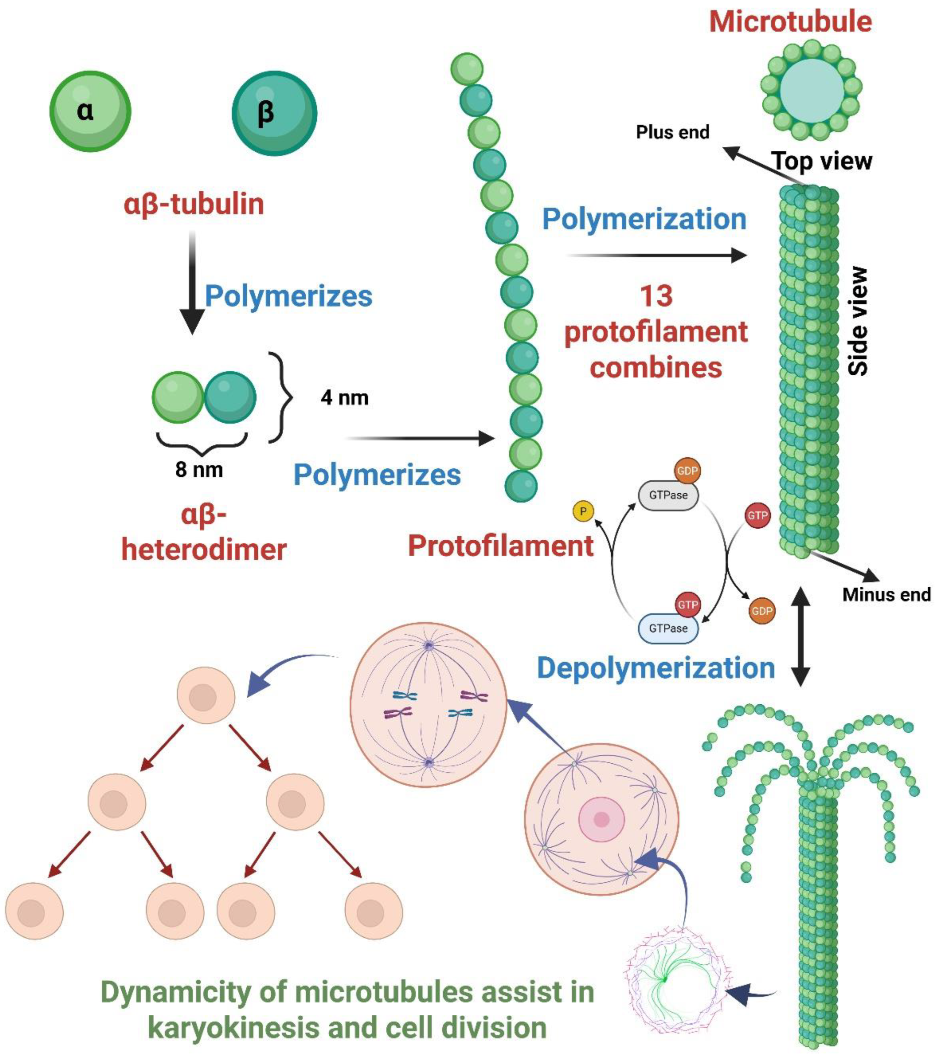
Figure 2.
A. The key druggable binding sites reported in the microtubules; B. Important drugs (approved and investigational) interacting at taxane, vinca, and colchicine binding sites.
Figure 2.
A. The key druggable binding sites reported in the microtubules; B. Important drugs (approved and investigational) interacting at taxane, vinca, and colchicine binding sites.
Scheme 1.
ML-driven computational drug repurposing workflow.
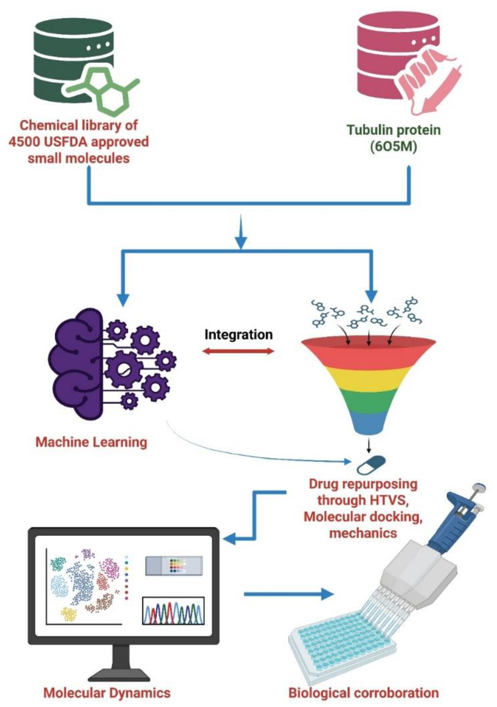
Figure 3.
X-ray crystal of tubulin in complex with the co-crystallized inhibitor G8K (PDB code: 6O5M). Chain A and Chain B of tubulin are coloured in pink and cyan, respectively, while the co-crystallized inhibitor is coloured in orange.
Figure 3.
X-ray crystal of tubulin in complex with the co-crystallized inhibitor G8K (PDB code: 6O5M). Chain A and Chain B of tubulin are coloured in pink and cyan, respectively, while the co-crystallized inhibitor is coloured in orange.
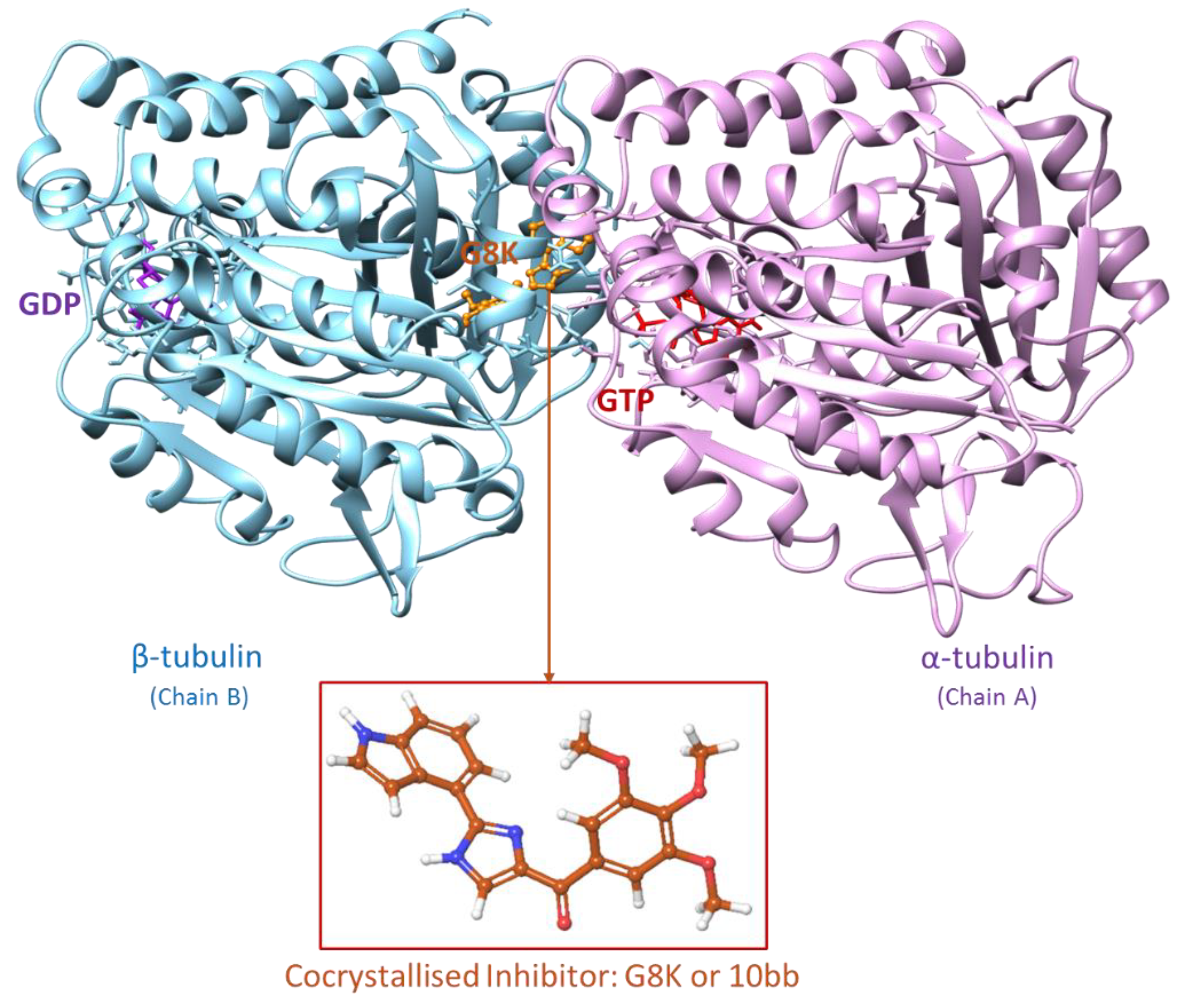
Figure 4.
Colchicine binding site (CBS) view of the tubulin protein, showing intermolecular contacts of the co-crystallized inhibitor G8K. (A) key residues are shown (B) all residues of the binding site are shown. G8K is coloured in orange, while the binding site residues are in blue.
Figure 4.
Colchicine binding site (CBS) view of the tubulin protein, showing intermolecular contacts of the co-crystallized inhibitor G8K. (A) key residues are shown (B) all residues of the binding site are shown. G8K is coloured in orange, while the binding site residues are in blue.
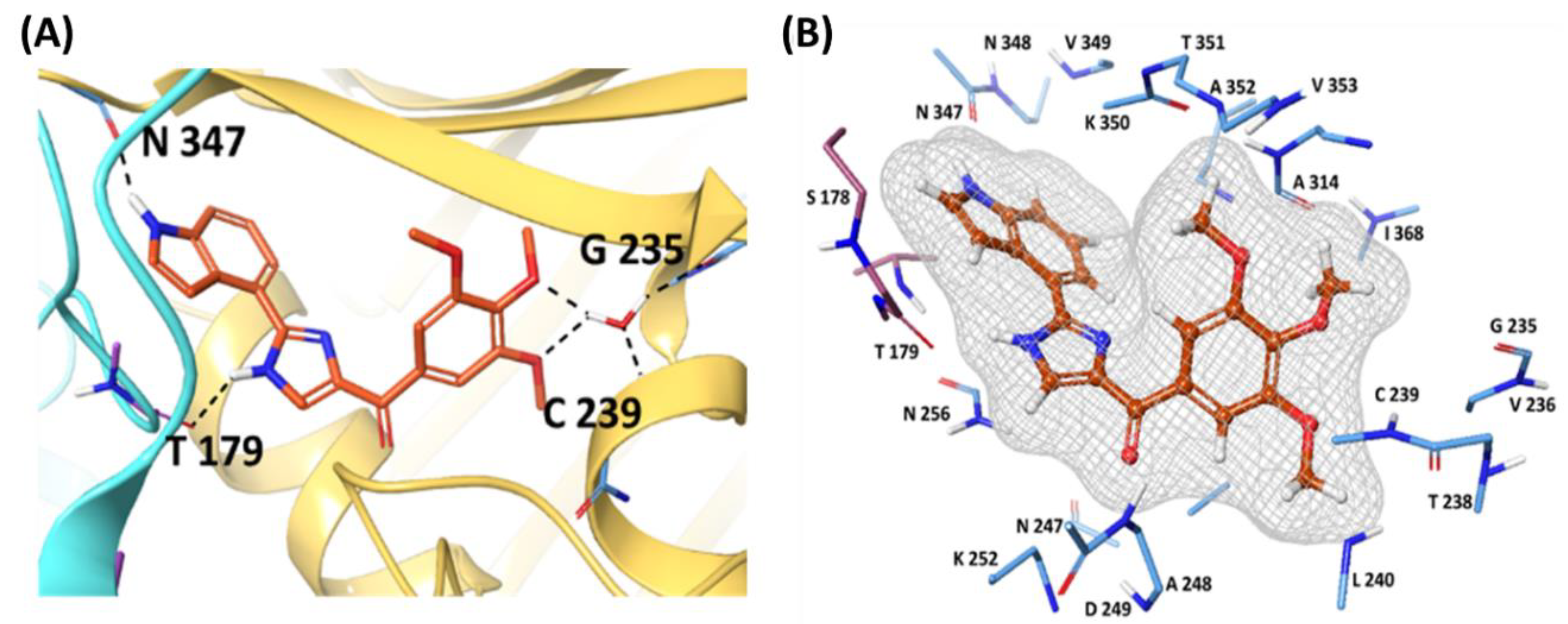
Figure 5.
Redocking study of the co-crystallized inhibitor G8K of tubulin. (A) The co-crystallized inhibitor pose is shown in orange. (B) The docking pose (Glide XP) is shown in green, perfectly superposed with the co-crystallized pose.
Figure 5.
Redocking study of the co-crystallized inhibitor G8K of tubulin. (A) The co-crystallized inhibitor pose is shown in orange. (B) The docking pose (Glide XP) is shown in green, perfectly superposed with the co-crystallized pose.
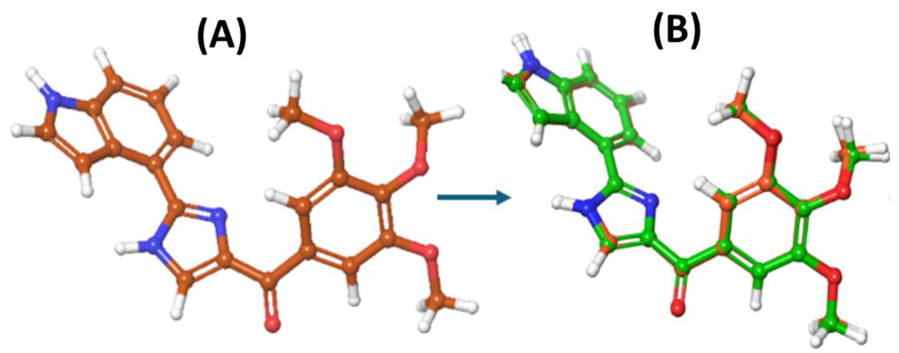
Figure 6.
Structure-based virtual screening workflow.
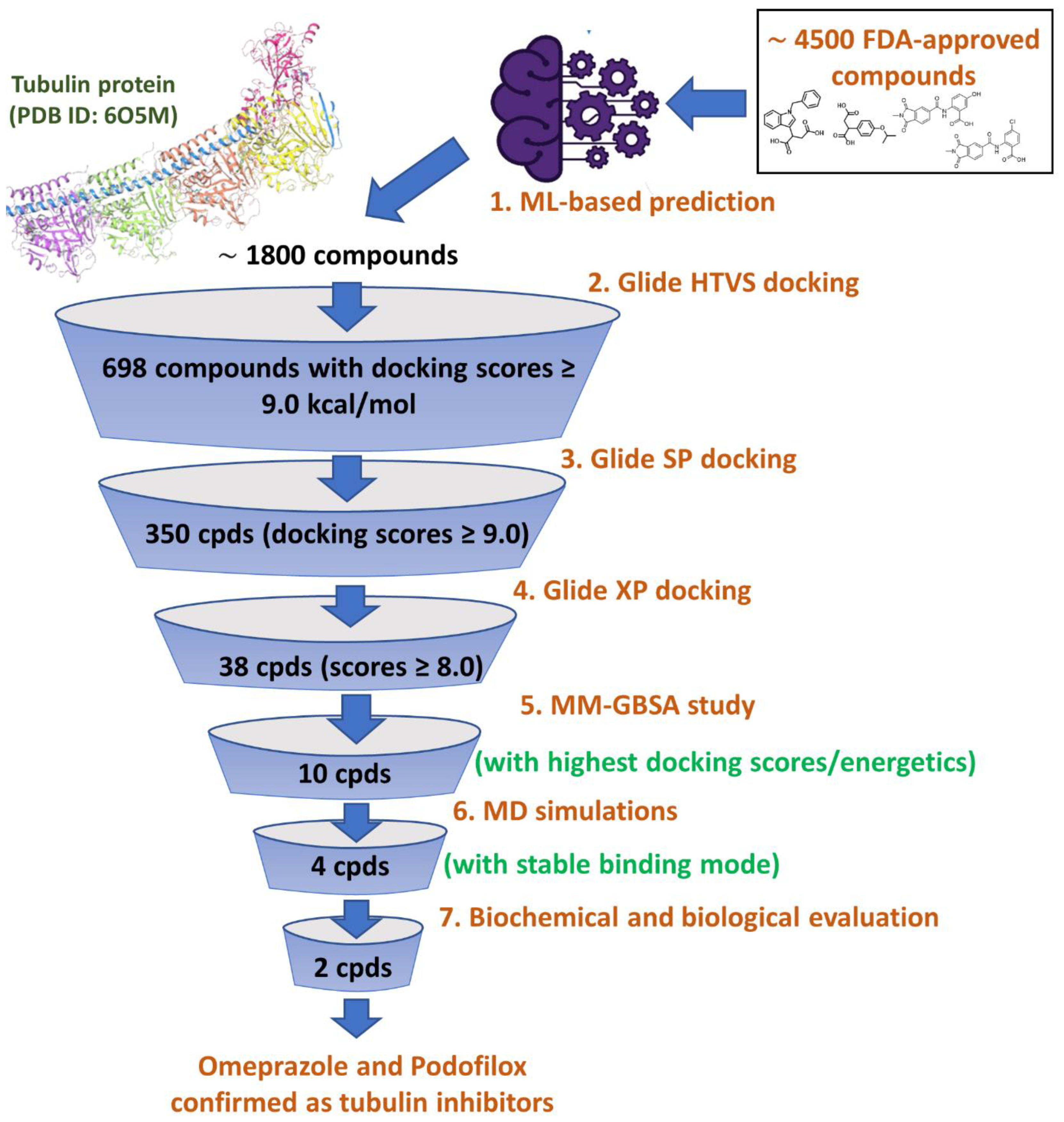
Figure 7.
Binding mode of Podofilox (green) representing 3D (A) and 2D (B) interactions in the colchicine binding site (CBS) of tubulin. .
Figure 7.
Binding mode of Podofilox (green) representing 3D (A) and 2D (B) interactions in the colchicine binding site (CBS) of tubulin. .
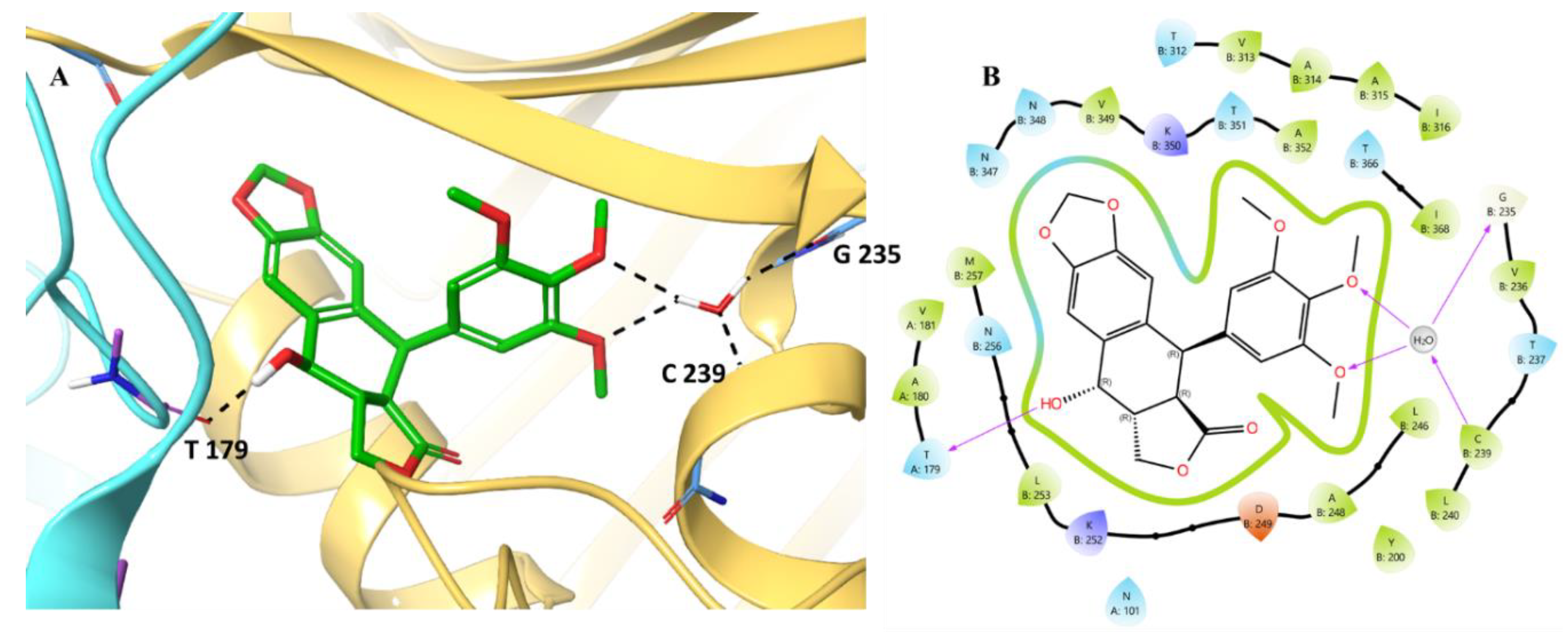
Figure 8.
Binding mode of Omeprazole (pink) representing 3D (A) and 2D (B) interactions in the colchicine binding site of tubulin. .
Figure 8.
Binding mode of Omeprazole (pink) representing 3D (A) and 2D (B) interactions in the colchicine binding site of tubulin. .
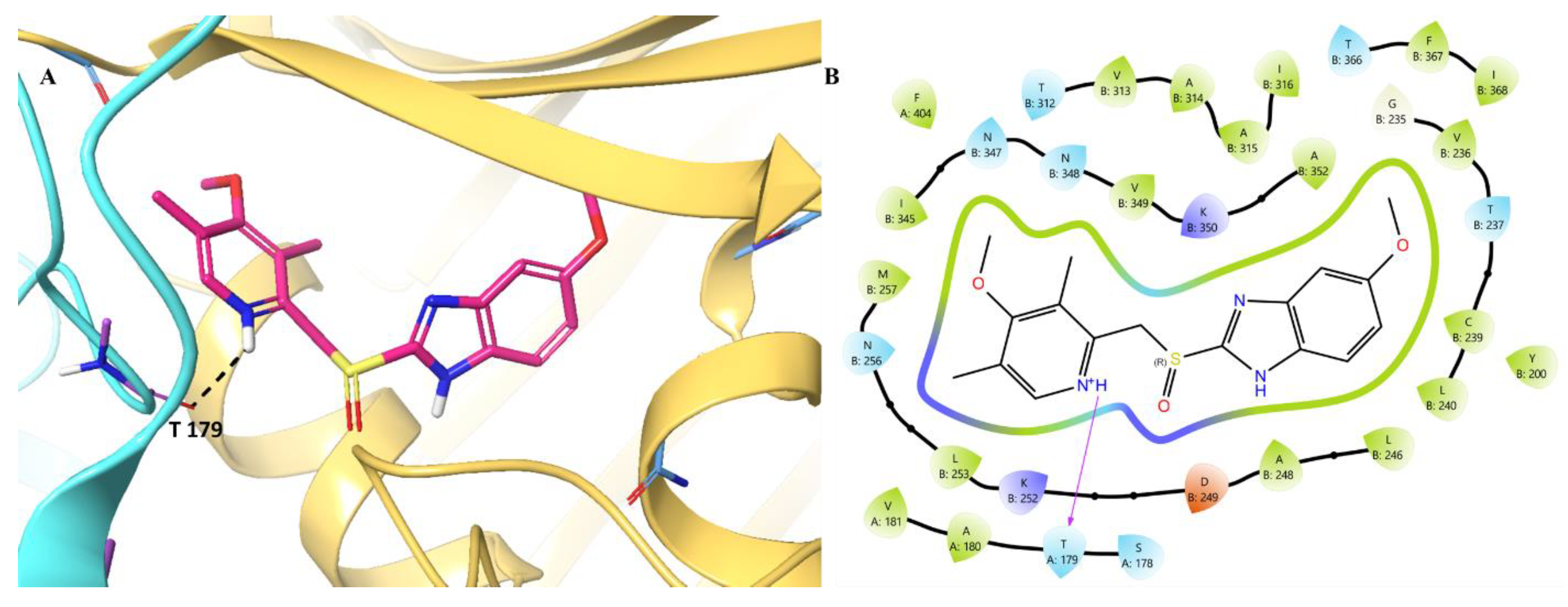
Figure 9.
Binding mode of Sulfadoxine (purple) representing 3D (A) and 2D (B) interactions in the colchicine binding site of tubulin.
Figure 9.
Binding mode of Sulfadoxine (purple) representing 3D (A) and 2D (B) interactions in the colchicine binding site of tubulin.
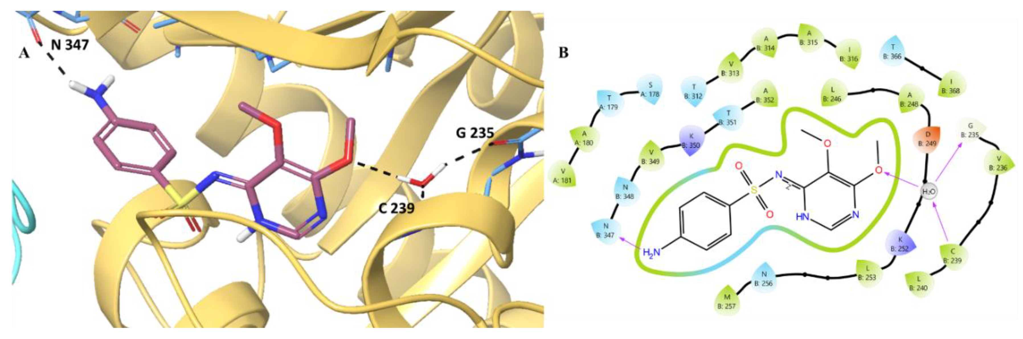
Figure 10.
Binding mode of Trimethoprim (brown) representing 3D (A) and 2D (B) interactions in the colchicine binding site of tubulin. .
Figure 10.
Binding mode of Trimethoprim (brown) representing 3D (A) and 2D (B) interactions in the colchicine binding site of tubulin. .
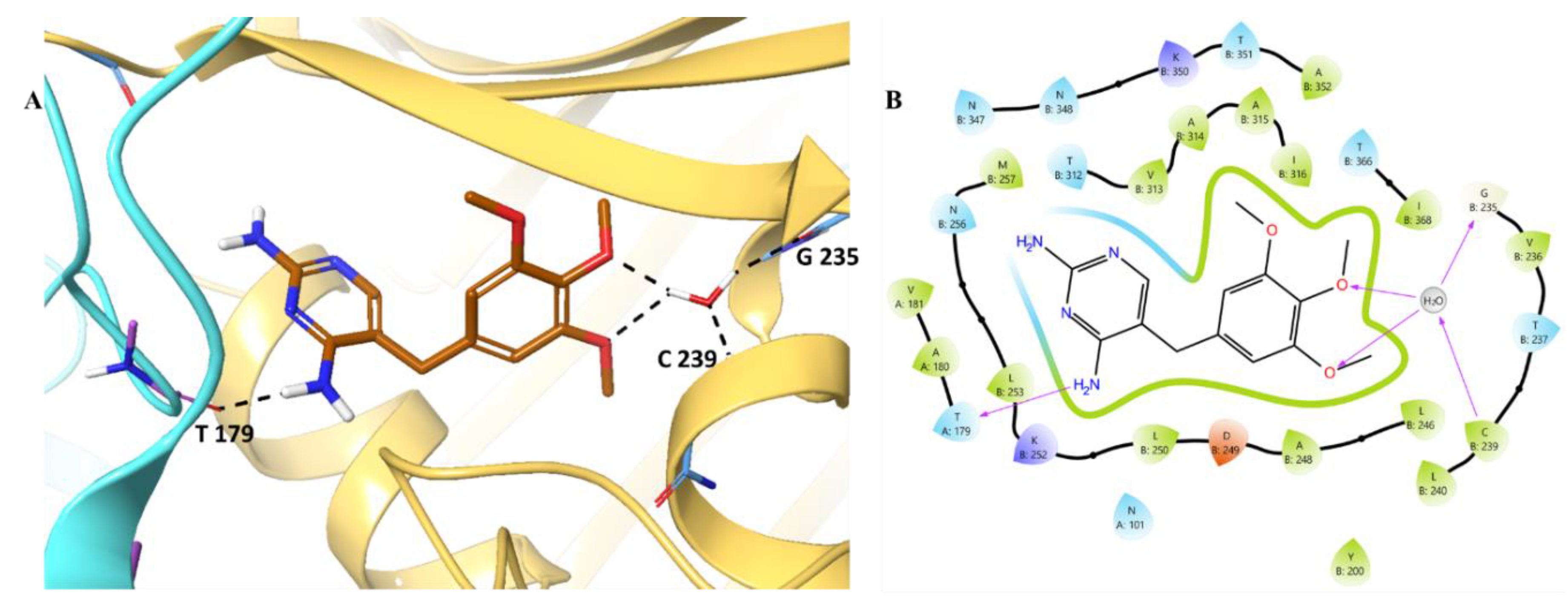
Figure 11.
(A) RMSD analysis of co-crystallized inhibitor (inhibitor in orange, protein α-carbons in dark blue) during the 200 ns simulation (B) Protein-ligand interaction histogram from the MD simulations of co-crystallised inhibitor in the tubulin binding site (H-bonds are shown in green, lipophilic contacts are shown in light purple and water bridges are represented in blue colour) (C) A schematic of detailed ligand atom interactions with the protein residues. Interactions that occur more than 30.0% of the simulation time in the selected trajectory (0.00 through 200 ns), are shown.
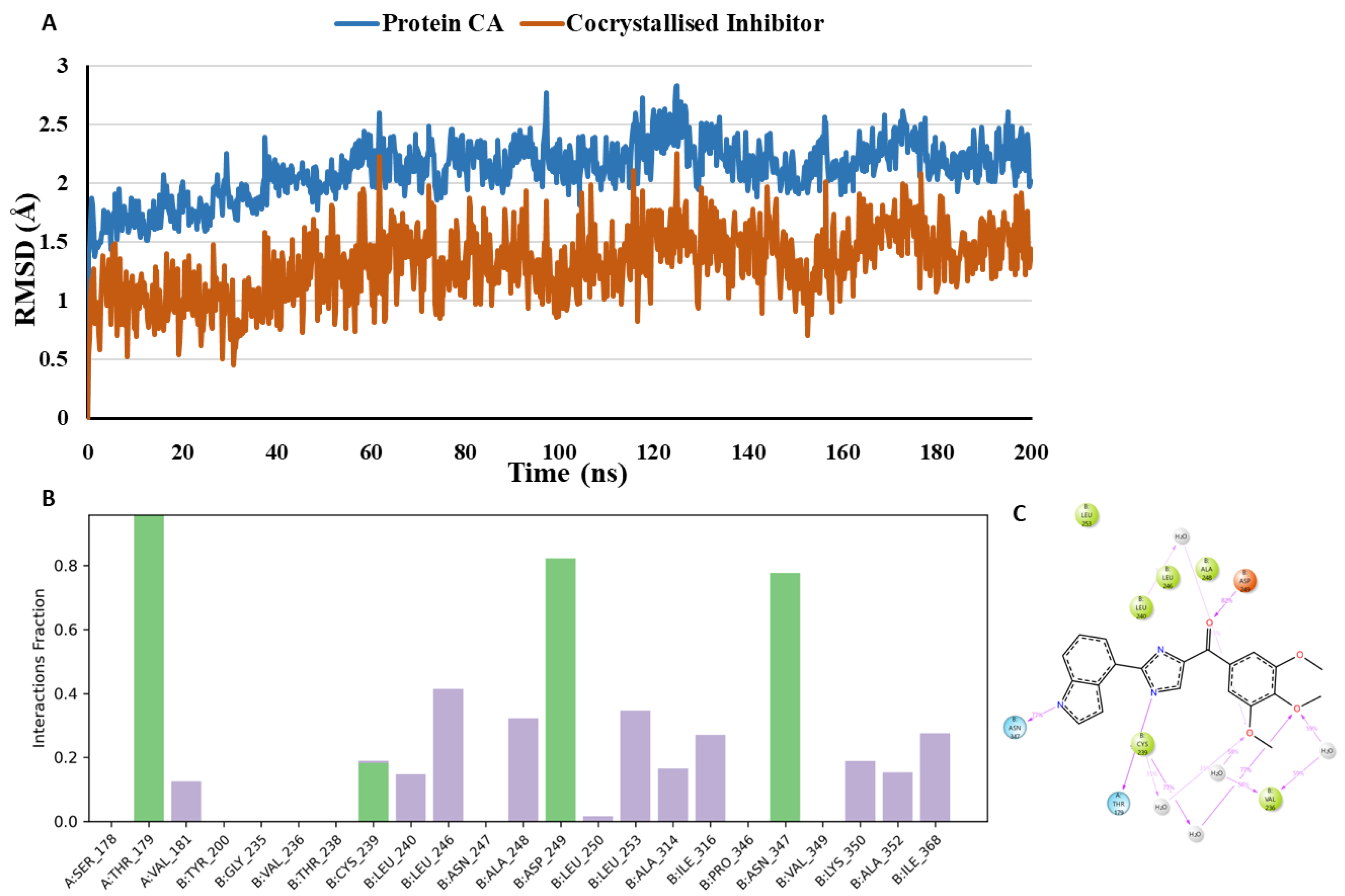
Figure 12.
(A) RMSD analysis of the docked compound podofilox (podofilox in green, protein α-carbons in dark blue) during the 200 ns simulation. (B) Protein-ligand interaction histogram from the MD simulations of podofilox in the tubulin binding site (H-bonds are shown in green, lipophilic contacts are shown in light purple and water bridges are represented in blue colour). (C) A schematic of detailed ligand atom interactions with the protein residues. Interactions that occur more than 30.0% of the simulation time in the selected trajectory (0.00 through 200 ns), are shown.
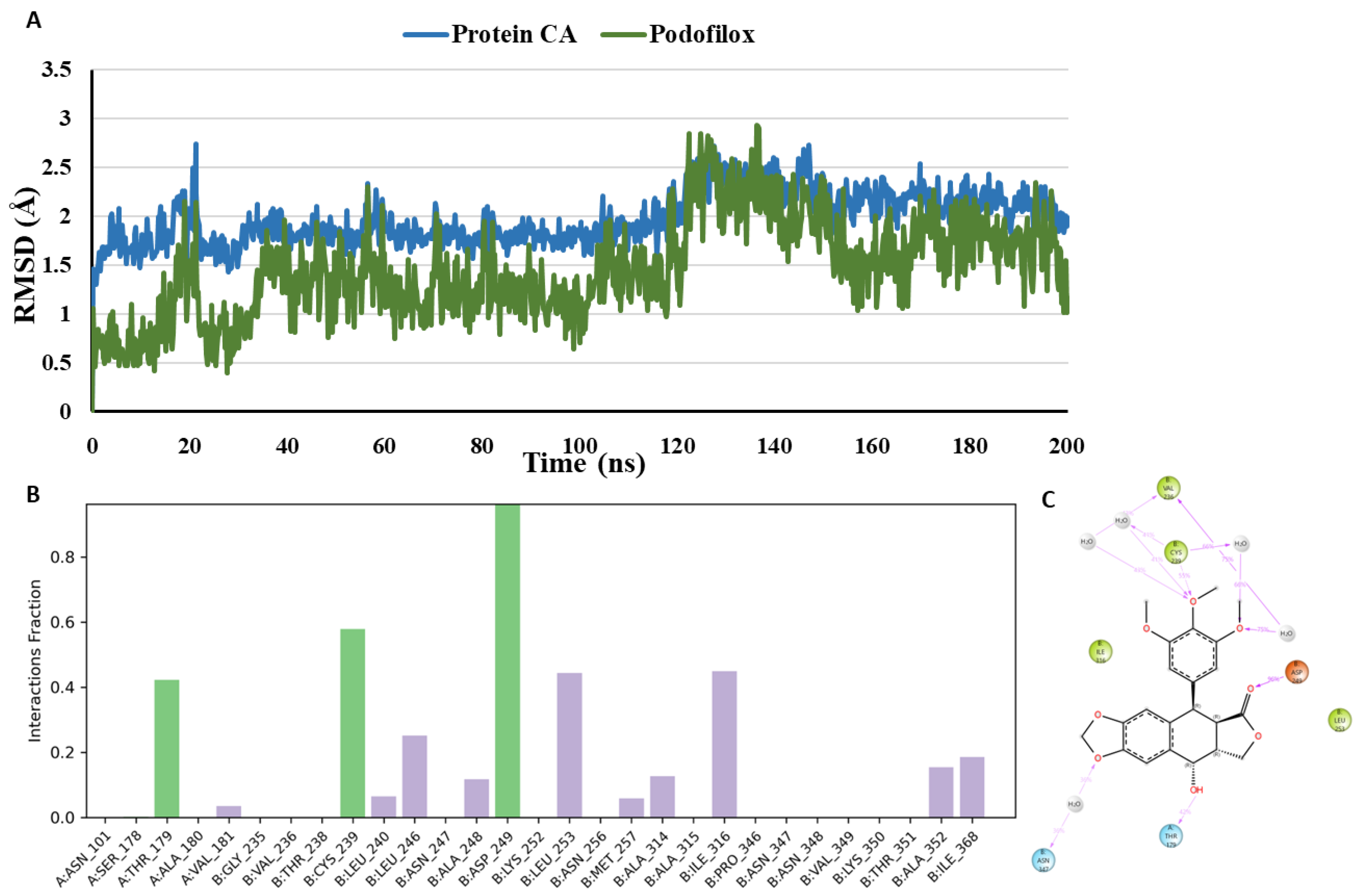
Figure 13.
(A) RMSD analysis of the docked compound omeprazole (omeprazole in pink, protein α-carbons in dark blue) during the 200 ns simulation. (B) Protein-ligand interaction histogram from the MD simulations of omeprazole in the tubulin binding site (H-bonds are shown in green, hydrophobic contacts are shown in light purple and water bridges are shown in blue colour). (C) A schematic of detailed ligand atom interactions with the protein residues. Interactions that occur more than 30.0% of the simulation time in the selected trajectory (0.00 through 200 ns), are shown.
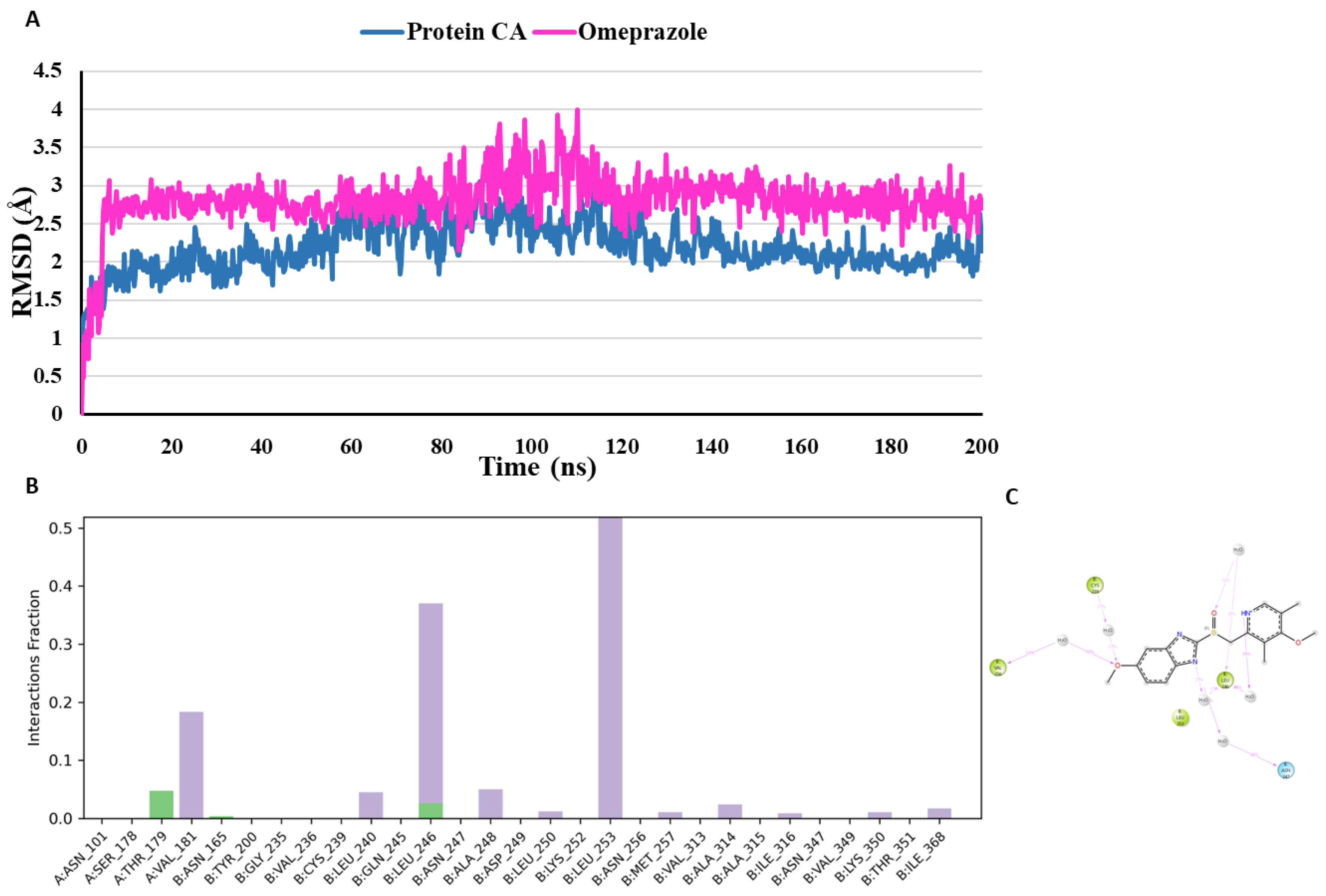
Figure 14.
(A) RMSD analysis of the docked compound sulfadoxine (sulfadoxine in purple, protein α-carbons in dark blue) during the 200 ns simulation. (B) Protein-ligand interaction histogram from the MD simulations of sulfadoxine in the tubulin binding site (H-bonds are shown in green, hydrophobic contacts are shown in light purple and water bridges are represented in blue colour). (C) A schematic of detailed ligand atom interactions with the protein residues. Interactions that occur more than 30.0% of the simulation time in the selected trajectory (0.00 through 200 ns), are shown.
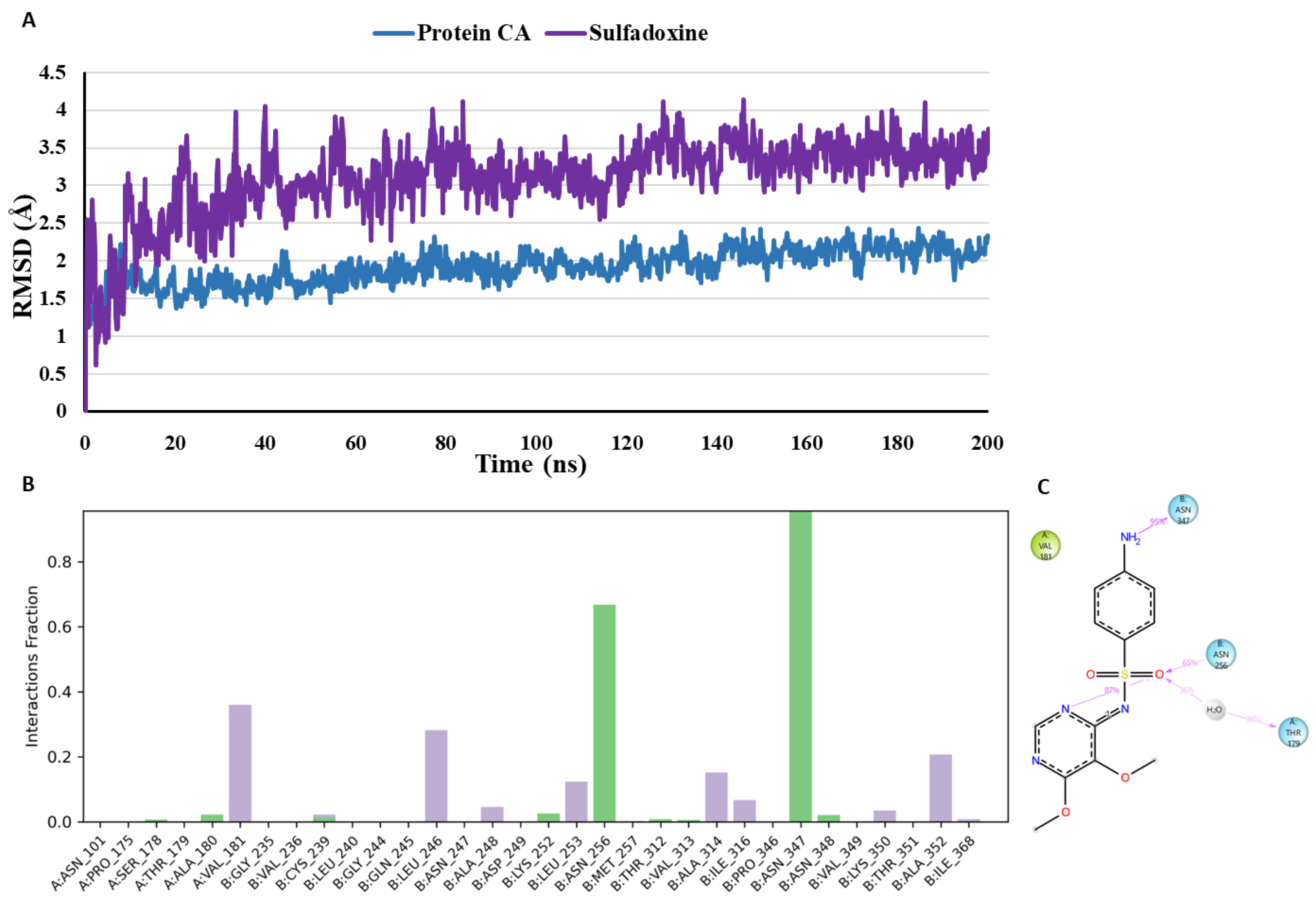
Figure 15.
(A) RMSD analysis of the docked compound trimethoprim (trimethoprim in brown, protein α-carbons in dark blue) during the 200 ns simulation. (B) Protein-ligand interaction histogram from the MD simulations of trimethoprim in the tubulin binding site (H-bonds are shown in green, hydrophobic contacts are shown in light purple and water bridges are shown in blue colour). (C) A schematic of detailed ligand atom interactions with the protein residues. Interactions that occur more than 30.0% of the simulation time in the selected trajectory ( 0.00 through 200 ns), are shown.
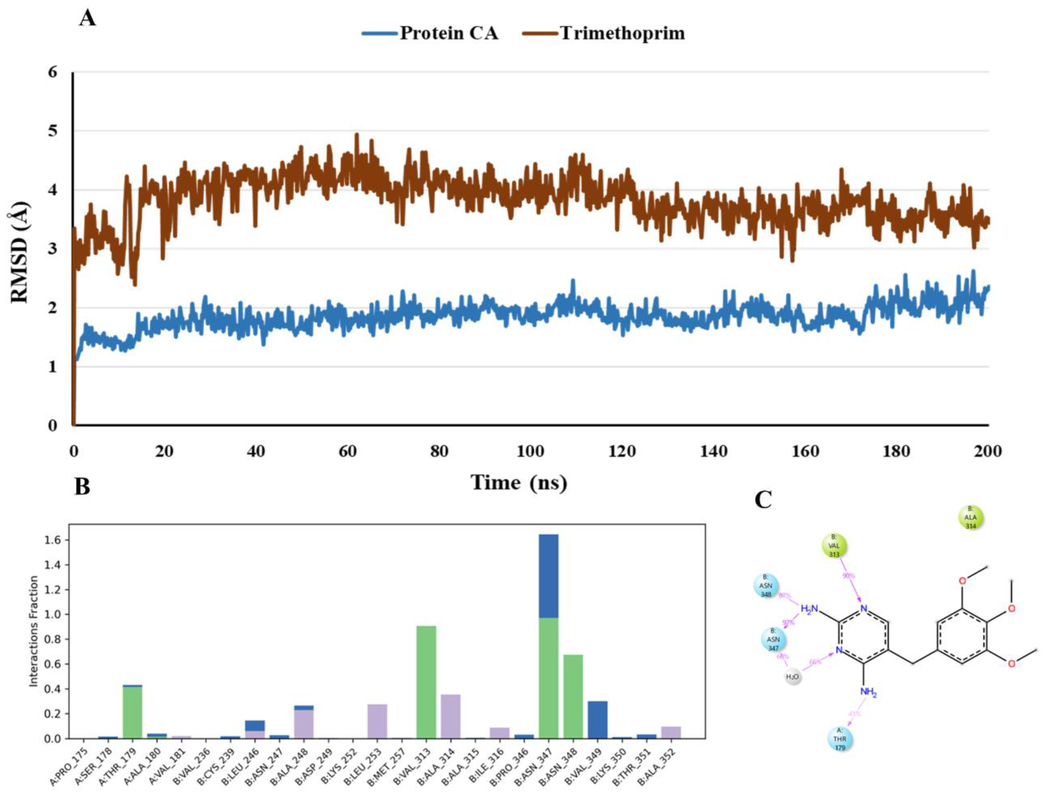
Figure 16.
Outcome of tubulin polymerization assay. The analysis revealed the compounds stabilized the microtubules, leading to a loss in their dynamicity and plausible inhibition (NC: Negative control).
Figure 16.
Outcome of tubulin polymerization assay. The analysis revealed the compounds stabilized the microtubules, leading to a loss in their dynamicity and plausible inhibition (NC: Negative control).
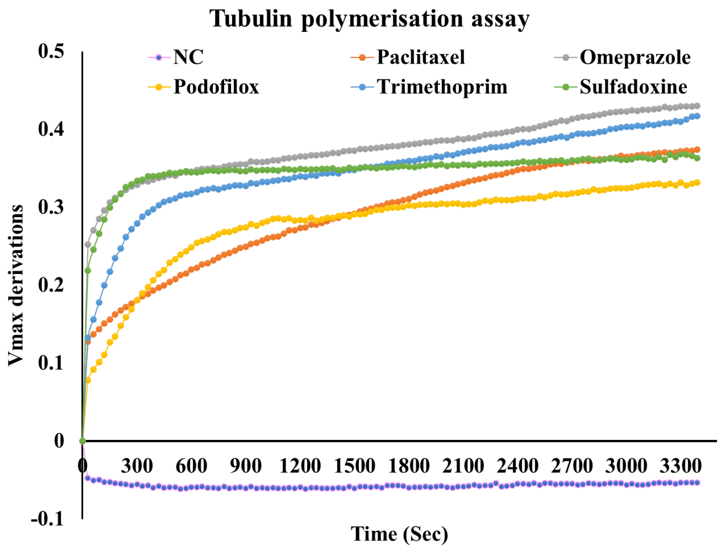
Figure 17.
Fluorescence analysis of F-actin organization (Green colour) in cells, along with DAPI staining (blue colour), following treatment with investigational hits, omeprazole, and podofilox, and positive control colchicine in HCT-116 cells in comparison to the untreated cells (control). The image also portrays the merged and contrast images for each intervention.
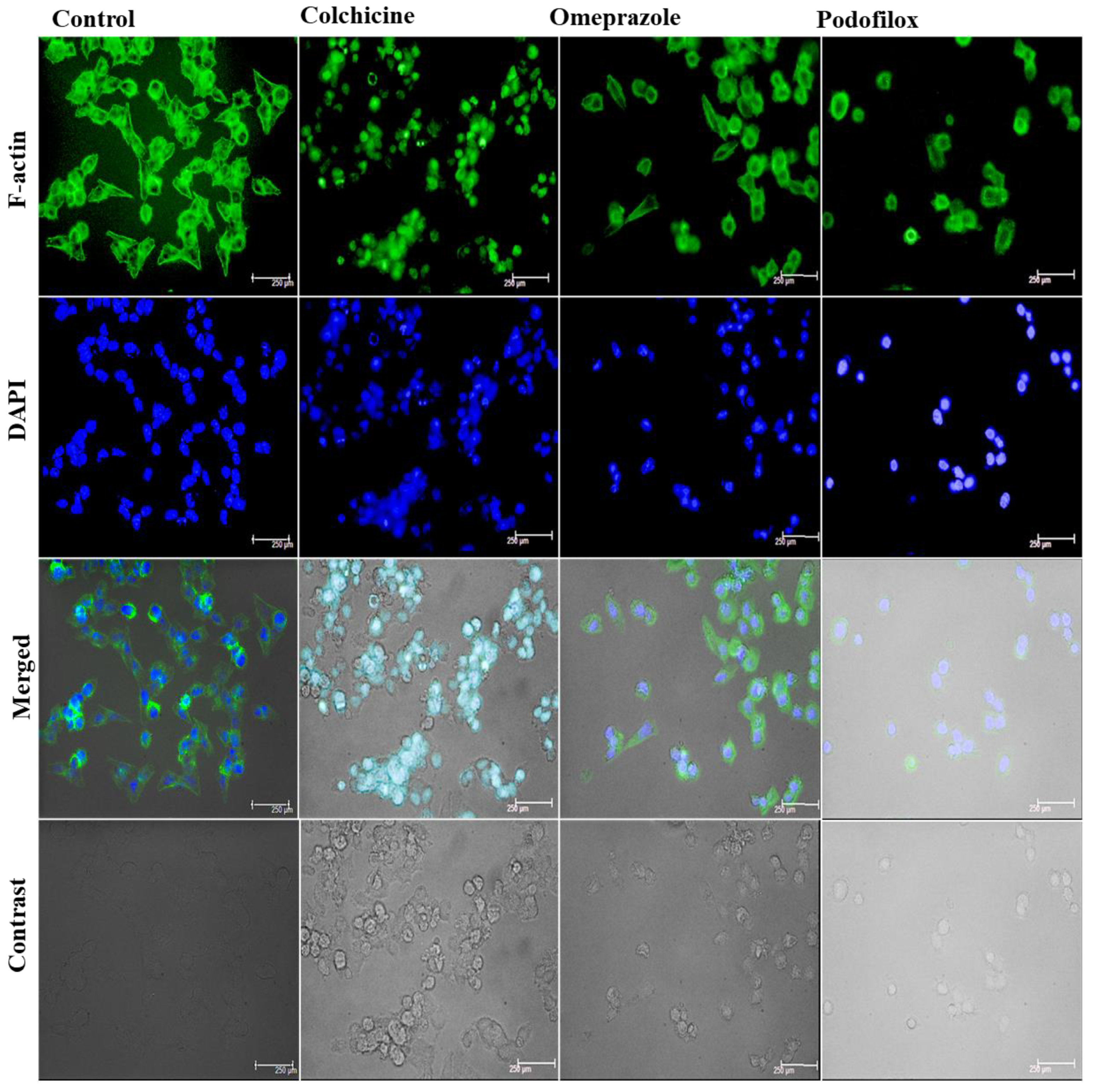

Table 1.
Performance of top 10 ML models for tubulin inhibitor classification.
| Entry | Model Name | Algorithm | Descriptor Type | Model Score |
| 1. | Bayes_dendritic_1 | Bayesian Classification | Dendritic Fingerprints | 0.9389 |
| 2. | Bayes_linear_20 | Bayesian Classification | Linear Fingerprints | 0.9337 |
| 3. | Bayes_linear_2 | Bayesian Classification | Linear Fingerprints | 0.9257 |
| 4. | Bayes_dendritic_2 | Bayesian Classification | Dendritic Fingerprints | 0.9256 |
| 5. | Bayes_linear_33 | Bayesian Classification | Linear Fingerprints | 0.9237 |
| 6. | Bayes_molprint2D_46 | Bayesian Classification | Mol2D Fingerprints | 0.9200 |
| 7. | Bayes_linear_1 | Bayesian Classification | Linear Fingerprints | 0.9185 |
| 8. | RP_30 | Recursive Partitioning | Mixed Descriptor Set | 0.9158 |
| 9. | Bayes_dendritic_33 | Bayesian Classification | Dendritic Fingerprints | 0.9146 |
| 10. | RP_41 | Recursive Partitioning | Mixed Descriptor Set | 0.9133 |
Table 2.
Performance of the best bayes regression model (bayes_dendritic_1).
| Dataset | RMS Err | Correlation (r) | R2/Q2 |
| Training | 0.2246 | 0.9045 | 0.8182 |
| Test | 0.2374 | 0.8988 | 0.8078 |
Table 3.
Performance of the recursive partitioning classification model (RP_30).
| Dataset | Class | TP | FP | TN | FN | Recall | Precision | Specificity | F-measure |
| Training set | Active | 125 | 11 | 78 | 4 | 0.969 | 0.919 | 0.876 | 0.943 |
| Inactive | 78 | 4 | 125 | 11 | 0.876 | 0.951 | 0.969 | 0.912 | |
| Test set | Active | 41 | 4 | 25 | 1 | 0.976 | 0.911 | 0.862 | 0.943 |
| Inactive | 25 | 1 | 41 | 4 | 0.862 | 0.962 | 0.976 | 0.909 |
Table 4.
Glide XP docking scores of top 10 compounds along with their binding energetics.
| Entry | Compound | Glide XP Docking Score (Kcal/mol) |
ΔGbind (Kcal/mol) |
ΔGcoulomb (Kcal/mol) |
| 1. | Arformoterol | -10.061 | -18.12 | -21.37 |
| 2. | Podofilox | -9.908 | -38.61 | -22.45 |
| 3. | Tretoquinol | -9.857 | -17.73 | -20.95 |
| 4. | Terizidone | -9.219 | -25.83 | -17.28 |
| 5. | Rucaparib | -9.145 | -19.46 | -15.23 |
| 6. | Aminoglutethimide | -8.99 | -26.59 | -6.77 |
| 7. | Sulfadoxine | -8.763 | -50.56 | 15.89 |
| 8. | Naftifine | -8.531 | -32.33 | -6.58 |
| 9. | Omeprazole | -8.362 | -64.16 | -58.31 |
| 10. | Trimethoprim | -8.117 | -43.89 | -18.9 |
| 11. | Co-crystallized G8K | -12.365 | -74.07 | -29.70 |
Table 5.
Half maximal inhibitory concentration (IC50) portrayed by identified hits in the panel of cancer cell lines.
Table 5.
Half maximal inhibitory concentration (IC50) portrayed by identified hits in the panel of cancer cell lines.
| Code | Half Maximal Inhibitory Concentration (IC50) (µM) ± SD | |||||
| SK-MEL-28 (Melanoma) |
A549 (Lung) |
MDAMB-231 (Breast) |
MCF-7 (Breast) |
PC-3 (Prostate) |
HCT-116 (Colon) | |
| Omeprazole | 4.32±0.29 | 17.32±0.19 | 21.65±0.21 | 13.44±0.26 | 12.22±0.18 | 6.22±0.22 |
| Podofilox | 4.98±0.37 | >25 | 19.83±0.24 | 13.61±0.18 | 15.93±0.31 | 5.76±0.18 |
| Trimethoprim | 7.46±0.19 | >25 | >25 | >25 | 18.65±0.28 | 11.32±0.31 |
| Sulfadoxine | 5.22±0.33 | >25 | 16.11±0.19 | 18.22±0.27 | 13.98±0.22 | 8.88±0.27 |
| Paclitaxel | 1.98±0.31 | 2.22±0.35 | 3.89±0.22 | 3.22±0.33 | 4.86±0.19 | NT |
| Colchicine | 2.43±0.19 | 2.11±0.22 | 2.54±0.31 | 2.89±0.24 | 4.02±0.16 | 4.92±0.19 |
Disclaimer/Publisher’s Note: The statements, opinions and data contained in all publications are solely those of the individual author(s) and contributor(s) and not of MDPI and/or the editor(s). MDPI and/or the editor(s) disclaim responsibility for any injury to people or property resulting from any ideas, methods, instructions or products referred to in the content. |
© 2025 by the authors. Licensee MDPI, Basel, Switzerland. This article is an open access article distributed under the terms and conditions of the Creative Commons Attribution (CC BY) license (http://creativecommons.org/licenses/by/4.0/).
Copyright: This open access article is published under a Creative Commons CC BY 4.0 license, which permit the free download, distribution, and reuse, provided that the author and preprint are cited in any reuse.


