Submitted:
13 August 2025
Posted:
14 August 2025
You are already at the latest version
Abstract
Understanding the dynamics of fire propagation is essential for improving predictive models and developing effective fire management strategies. This study examines the variability in temporal and directional rates of spread (ROS) under controlled environmental conditions and investigates the influence of terrain slope using experimental fire videos. To enable precise, frame-by-frame tracking of fire perimeters, we employed the Segment Anything Model (SAM) for semantic segmentation and object tracking, allowing us to quantify fire spread. Our study highlight that ROS exhibited substantial variability across and within videos that underscore the stochastic nature of fire behavior and raise concerns about the limitations of deterministic fire spread models. Analysis of the slope spread factor revealed discrepancies between model predictions and observed fire behavior. Estimated slope parameters deviated from values reported in existing literature, suggesting that fire dynamics are highly context-dependent and sensitive to local conditions. Our work highlights the need for probabilistic modeling approaches that explicitly account for inherent uncertainty and emergent dynamics in fire spread. Future research should focus on integrating directional drivers, refining slope-response formulations, and incorporating stochastic processes such as spotting. These improvements are essential for building more robust and generalizable fire behavior models capable of supporting operational forecasting and management decisions.
Keywords:
ate of spread
; fire behaviour
; segmentation
; stochastic
; mixed models
1. Introduction
Wildfires can lead to severe environmental, economic, and social consequences. The frequency and severity of wildfires have increased globally in recent decades, owing to variables such as climate change, land-use patterns, and extended dry seasons [1]. As wildfires become more frequent and destructive, the demand for accurate and robust fire spread models has become increasingly urgent.
One of the central challenges in wildfire modelling is accurately predicting fire spread while accounting for the uncertainties inherent in natural processes. In Canada, widely used fire modelling systems such as the Canadian Forest Fire Behaviour Prediction (FBP) System [2] and the Prometheus wildfire growth simulator [3] are grounded in deterministic frameworks. While operationally effective, these models are built on a relatively narrow empirical foundation, drawing primarily from controlled field experiments and selected case studies aligned with the Canadian Forest Fire Weather Index (FWI) System [4]. As a result, they can fail to capture the stochastic nature of fire behavior and environmental variability, leading to discrepancies between predicted and observed fire dynamics, particularly under rapidly evolving or extreme conditions.
Satellite remote sensing offers a promising supplement to ground-based fire modelling. Instruments such as Moderate Resolution Imaging Spectrometer (MODIS) and Visible Infrared Imaging Radiometer Suite (VIIRS) provide near real-time fire detection [5], while higher-resolution platforms like Sentinel-2 enable detailed burn area mapping [6]. These tools are especially valuable for identifying fires in remote and inaccessible regions. However, they face several limitations that restrict their effectiveness for continuous fire behaviour monitoring. Most Earth observation satellites pass over Canadian latitudes only once or twice per day, typically during late morning or early afternoon, often missing the late-afternoon to evening period when fire activity tends to peak [7]. In addition, data latency can range from several hours to days, and coarse spatial resolutions limit the ability of the sensors to capture fine-scale fire dynamics. This limitation is particularly critical for fires occurring near the wildland–urban interface, where small-scale variations in fire behaviour can have disproportionate impacts on infrastructure, human safety, and evacuation decision-making[8].
Given these constraints, our study is motivated by the need for a more granular and temporally responsive approach to understanding fire spread. We leverage experimental fire videos recorded under controlled conditions to capture the real-time evolution of fire perimeters.While such burns are necessarily small-scale and cannot fully replicate the complexity of wildland fires or satellite observations, they provide a valuable proxy for assessing what types of fire behaviour may become observable as remote sensing technologies continue to improve in resolution and revisit frequency. By analyzing these controlled burns, we aim to characterize the variability in the ROS and highlight the importance of incorporating stochasticity into fire modelling frameworks. In particular, we find that characterizing rate of spread may be a challenge that will require disaggregation as tech improves. Ultimately, our goal is to inform the development of probabilistic, data-driven models that better reflect the dynamic and uncertain nature of fire behaviour.
The remainder of this paper is organized as follows. Section 2 reviews related work in fire spread modelling, with a focus on deterministic frameworks and recent advancements and efforts to incorporate uncertainty. Section 3 describes the experimental video datasets and outlines the data collection process. Section 4 presents our methodology, which combines segmentation-based fire perimeter tracking with statistical models for assessing ROS. Section 5 reports the results of our analysis, demonstrating how our approach captures spread variability and reveals the limitations of existing models. Finally, Section 6 concludes the paper and discusses future directions.
2. Related Work
Wildfire modelling covers a diverse range of approaches tailored to different objectives, data availability, and computational capacities. Empirical models rely on statistical relationships derived from historical fire behaviour and environmental conditions. Widely used systems like the Fire Weather Index, [4] and Canadian Fire Behaviour Prediction [2] rely on empirical equations derived from field and laboratory studies, predicting fire spread based on fuel types, weather conditions, and topography. They provide practical predictions of fire spread and intensity, though their reliance on historical patterns limits adaptability to novel conditions. There are also semi-empirical models, such as BEHAVE Plus [9] and Prometheus [3], which combine statistical relationships with simplified physical principles to improve balance between accuracy and computational efficiency, often serving operational fire management and wildfire risk assessment services. Another work has further enhanced PROMETHEUS by introducing statistical smoothing and a residual-based bootstrap method, improving both accuracy and enabling stochastic fire spread simulations [10]. Other studies have addressed geometric instabilities in the evolving fire front, proposing outer hull and level set methods to enhance numerical robustness [11].
Physical and deterministic models such as FIRETEC and the Wildland–Urban Interface Fire Dynamics Simulator (WFDS) simulate fire behaviour based on fundamental physical principles, offering detailed representations of heat transfer, combustion, and fire–atmosphere interactions [12]. While these models provide valuable insights into the physics of fire propagation, their high computational cost severely limits their use in real-time applications. Furthermore, deterministic models often fail to capture the inherent variability and stochastic nature of fire behaviour, which can lead to overconfident predictions and reduced effectiveness in operational decision-making [13,14].
To address these limitations, researchers have developed stochastic and probabilistic models that explicitly account for uncertainty. Tools such as FlamMap [15], FSim [16], and Dionysus [17] simulate potential fire scenarios using probabilistic methods, making them well-suited for wildfire risk assessments. Dionysus, for example, extends the deterministic PROMETHEUS model by generating probability contours around predicted fire fronts using statistical modelling of input uncertainties. Other models introduce stochasticity directly into fire growth dynamics, capturing not only average behaviour but also variability in spread, spotting, and event timing [18]. Beyond model development, researchers have also proposed evaluation frameworks to assess whether stochastic simulators reflect real-world variability. One such approach compares the simulated rate-of-spread variability with that of observed experimental fires, offering a path toward more robust validation of fire spread uncertainty[19].
Machine learning approaches, including neural networks and random forests, have been increasingly applied to wildfire susceptibility mapping, real-time detection, and predictive modelling [20]. These models leverage large environmental and historical datasets, though their performance hinges on data quality and coverage. Another class of models—cellular automata represents landscapes as spatial grids with rule-based transitions among neighbouring cells [21,22]. While computationally efficient and useful for spatial dynamics, they simplify many physical and environmental processes. More recent advancement in fire modelling involves image-based segmentation, which supports fire detection and behaviour analysis by isolating fire-affected regions in aerial and satellite imagery [23,24]. Classical methods such as thresholding, edge detection, and region-growing have long been used to delineate fire perimeters from thermal or optical inputs [25]. More recently, deep learning, particularly convolutional neural networks (CNNs), has enabled pixel-level classification through architectures like Fully Convolutional Networks (FCNs) [26] and U-Net [27]. Newer models such as U-Net and YOLOv7 have demonstrated strong performance in noisy, occluded environments, supporting real-time wildfire monitoring [28,29,30]. Emerging tools such as the Segment Anything Model (SAM) [31] further reduce the overhead of manual annotation, offering a general-purpose framework capable of identifying fire-related regions with minimal supervision. Integrating segmentation techniques with existing wildfire modelling frameworks enables more detailed and responsive representations of fire behaviour, opening new directions for data-driven fire prediction and risk assessment.
Environmental factors such as temperature, moisture content, wind speed, and slope are key determinants of wildfire behavior, directly influencing the rate of spread (ROS) and combustion dynamics [32]. Higher temperatures and lower moisture levels reduce ignition thresholds and accelerate combustion, while fuel drying times affect the flammability of surface materials. Slope further amplifies fire spread by preheating uphill fuels via radiation and convection, resulting in increased ROS at the upslope front [33,34]. Despite these well-understood effects, the interactions among environmental variables remain complex and context-dependent, contributing to substantial variability in fire behaviour. This variability poses significant challenges for wildland fire management and modelling. The stochastic nature of fire propagation, combined with limitations in data availability, ecological knowledge, and metrics for evaluating assets at risk, introduces uncertainty into both operational forecasting and long-term planning [35]. Moreover, dynamic disturbance regimes and climate change further complicate predictive efforts. These uncertainties underscore the need for modelling frameworks that can account not only for environmental drivers but also for the variability and randomness inherent in fire behaviour.
Mixed-effects models provide a robust framework for addressing uncertainty in fire behaviour by simultaneously incorporating fixed effects (e.g., temperature, slope) and random effects (e.g., variation across regions or experimental replicates). This structure enables researchers to isolate systematic environmental drivers while accounting for unexplained variability [36]. For instance, Finney et.al[37] applied generalized mixed-effects regression to model fire containment probability, treating containment as a fixed effect and individual fires as random effects. Another paper demonstrated the effectiveness of mixed models for forest fire risk forecasting[38], as well as a separate study [39] showed that negative binomial mixed models can accommodate overdispersed wildfire occurrence data. Experimental fire studies by [40] further highlight the value of mixed modelling in distinguishing the effects of controlled variables from intrinsic stochastic behaviour. These models not only quantify variability but also provide probabilistic intervals for predictions by estimating variance components tied to fixed and random effects. This makes them well-suited for probabilistic fire growth modelling and informed decision-making in fire management. When combined with precise segmentation techniques, these models can further enhance their predictive capacity. Together, this integrated approach offers a robust framework for capturing environmental drivers of fire behaviour and managing the uncertainty inherent in wildfire dynamics.
3. Experimental Setup and Data Collection
The video data analyzed in this study was obtained from two distinct series of laboratory fire experiments [41,42] originally designed to serve as a mouse model of smouldering fire behavior. The experimental design systematically varied key environmental conditions that align with the three principal input categories of generic fire behavior prediction models:weather, topography, and fuel.
The combustion experiments were conducted on chemically treated wax paper substrates. The wax paper was immersed in a potassium nitrate solution and dried at temperatures between 50–70F for 60–120 minutes. This substrate served as a proxy for a single fuel type with a fixed chemical composition but variable pre-burn moisture content. Slope was manipulated across varying inclinations, simulating the effect of terrain on fire acceleration.
The potassium nitrate treatment served multiple purposes: it ensured uniform ignition, suppressed rapid flaming, and promoted sustained smouldering combustion. These conditions enabled mostly unobstructed observation of fire perimeter evolution throughout the burn sequence. The surface of the wax paper also exhibited irregularity and structural variation, offering a physically heterogeneous medium that replicates certain aspects of natural fuel beds.
Ignition was consistently initiated at the centre of the substrate using a directable ignitor within a fire-safe fume hood. The combustion process was recorded using a fixed overhead camera, capturing a top-down view of fire spread. Videos were recorded at a resolution of 320 × 240 pixels with a frame rate of 15 frames per second, and a spatial scale of 1.2 mm per pixel.
3.1. Micro-Structural Heterogeneity in the Fuel Bed
Although the fuel was macroscopically uniform in material composition, it served as a standardized analog of a natural fuel commonly used in fire behaviour models. Scanning Electron Microscopy (SEM) conducted by the original experimenters revealed notable micro scale structural heterogeneity in the treated wax paper and showed irregular distributions of pores, fibres, and surface textures[41]. Figure 1 illustrates this heterogeneity. This micro structural complexity is analogous to conditions found in natural forest environments, where the fuel bed comprises a mosaic of litter, twigs, decomposing organic matter, and soil particles, each with distinct combustion properties. Even within a single classified fuel type (e.g., C-1 or O-1a used in FBP), significant sub-fuel-type variation can influence ignition, heat transfer, and rate of spread.
The presence of structural heterogeneity in an otherwise uniform fuel type highlights a critical limitation of conventional fire behaviour modelling. Most operational systems, including FBP, treat fuel type as a categorical and internally homogeneous input, assuming that all instances of a fuel class will behave similarly under the same weather and topographic conditions. Our study challenges this assumption by investigating how stochastic fire behaviour can emerge even in controlled laboratory burns.
3.2. Data Generation
Using the experimental fire videos, we constructed two distinct datasets of fire spread distances. The first dataset collected data from 10 videos. To standardize the data across videos, a consistent frame selection method was applied based on each video’s ignition time (), defined as the first frame showing visible combustion. For each video, we identified the valid frame window in which fire spread occurred without reaching the substrate edge. A shared analysis range was then computed by taking the maximum lower bound and minimum upper bound of available frames across all videos, resulting in a fixed interval of 388 frames (approximately 25 seconds). This window begins after ignition and excludes the highly variable early flame dynamics. By aligning all videos to a stable phase of fire development, the selected interval approximates the quasi-equilibrium state typically used to report rate of spread in wildfire modeling systems such as the Canadian FBP System.
To isolate the effect of terrain inclination, the second dataset was created from slope variation trials[42]. These included burns conducted on inclines ranging from 5° to 50° in 5° increments, with all other environmental parameters held constant. This design ensured that any differences in rate of spread could be attributed solely to changes in slope, eliminating confounding factors. The same preprocessing steps were applied to these videos to extract spread distances over a matched time window.
4. Methodology
The methodology of the current study is organized into three main components. First, we focus on the segmentation of fire regions within experimental video frames using a vision transformer approach to accurately delineate the burning area over time. Second, we compute the ROS by quantifying the spatial progression of the fire perimeter across sequential frames. Third, we perform statistical analysis to assess the fire spread behaviour using environmental factors, such as temperature, dry time, and slope.
4.1. Segmentation of Fire Regions
To extract fire regions from smouldering fire videos, we developed a segmentation pipeline structured into three stages: pre-processing, segmentation, and post-processing.
Pre-processing involved identifying the ignition frame, the first appearance of fire in each video, and defining the ignition point coordinates. Assuming an approximately elliptical fire spread, this centre of the fitted ellipse was used as a point-based prompt to consistently guide segmentation across all frames.
Segmentation was carried out using the Segment Anything Model (SAM), a Vision Transformer-based architecture (ViT-H) pretrained for general-purpose image segmentation. The prompt and corresponding video frames were passed to the model, which returned the highest-confidence mask for each frame. All computations were performed in a GPU-enabled environment using pre-trained weights (sam_vit_h_4b8939.pth).
Lastly, to extract fire perimeter boundaries from grayscale SAM output, we applied a series of post-processing steps. First, each frame was converted to a binary mask using a fixed threshold (127), then to suppress high-frequency noise and preserve edge structures, a median filter [43] with a kernel size of 5 was applied to the binary images. The denoised binary masks were subsequently processed using a binary dilation operation to reinforce the continuity of the fire regions and mitigate fragmentation. Perimeter boundaries were delineated by performing a pixel-wise exclusive disjunction (XOR) between the dilated and original binary masks, yielding a precise representation of the fire front edges which were used as the basis for quantifying fire growth over time. Figure 2 illustrates the segmentation pipeline.
4.2. Rate of Spread Calculation
The fire perimeter is conceptually divided into three regions: the head, flanks, and rear, each reflecting distinct fire dynamics. The head of fire is the fastest-advancing section, typically aligned with wind direction or slope, and is often the primary focus in fire behaviour prediction systems. The flanks, positioned on the lateral edges, usually spread more slowly but can respond dynamically to shifting wind or terrain. The rear, opposite the head, exhibits the slowest spread due to less favourable burning conditions. Accordingly, ROS was initially calculated with respect to the head of the fire, representing the maximum outward expansion from the ignition point over time. This head-based ROS definition aligns with standard practice but, as discussed later, presents limitations under experimental conditions and irregular fire shapes. Initially, to compute ROS during the interval , we first identified the head of the fire, defined as the location of the most significant forward spread between two frames. This was achieved using a max–min distance approach: for each pixel in the later frame (), we calculated the Euclidean distance to all fire pixels in the earlier frame () and recorded the minimum distance to any pixel in . The pixel in with the maximum of these minimum distances was designated as the fire head.
To ensure consistent directional distance calculations, the horizontal angle of the vector to the identified head of the fire was used to rotate both frames, aligning the head with the positive x-axis. This standardization is necessary because the rear and flank directions are defined relative to the head, and a consistent frame of reference is required to compute directional spread meaningfully. After rotation, a bounding box was fitted to the fire region in each frame, and spread distance along the head, rear, and flanks was calculated based on changes in the bounding box margins. See Appendix A for a pseudocode summary of this ROS calculation procedure.
However, we noticed that even during what appears to be an equilibrium phase of fire spread, especially in small-scale controlled burns, the direction of the fire’s head can fluctuate within a single event. This variability prevents standardized tracking of fire progression and complicates head-based ROS and comparative modelling of ROS. Figure 3a shows an example of this behaviour. This observation challenges the assumption of a stable head direction over time and highlights the limitations of head-based ROS definitions. These inconsistencies underscore the need for more robust, direction-agnostic approaches to quantifying fire spread. To overcome the limitations, we implemented a complementary strategy designed to enable robust analysis of fire spread throughout our experiment.
4.2.1. Our Revised ROS Calculation Approach
To quantify the directional ROS, we computed the displacement of the fire perimeter across successive frames using the margins of the segmented fire region’s bounding box. Each frame was analyzed to extract the minimum and maximum pixel coordinates of the active fire mask along both the x-axis (horizontal) and y-axis (vertical) of the image plane. By measuring the change in these bounding box edges between consecutive frames, we obtained estimates of directional fire progression.
Specifically, directional ROS was calculated independently along the four cardinal directions of the image plane: upward and downward (along the y-axis) and leftward and rightward (along the x-axis). These directions correspond to the top, bottom, left, and right margins of the bounding box, respectively. Figure 3b illustrates our revised ROS approach. This coordinate-based formulation enables the detection of anisotropic spread dynamics without relying on external spatial references such as wind or slope direction. For each video, directional spread distances were computed at 1-second intervals over a fixed 25-second analysis (388 available frames) window by comparing the bounding box margins of the segmented fire region across consecutive frames. This yielded 25 time-stamped measurements per direction, per video, resulting in a structured dataset suitable for assessing the fire spread dynamics across varying environmental conditions.
For the slope-focused experiments, we restricted the analysis to two directional ROS components aligned with the slope: rightward (upslope) and leftward (downslope) along the x-axis of the image plane. Specifically, we measured the time required for the fire front to traverse a fixed distance of 100 pixels along this axis. This targeted approach allowed us to isolate and assess the influence of terrain inclination on fire spread rate and directionality. Some recordings, such as those at 35 degrees were excluded from the dataset due to incomplete fire propagation. All spread distances were subsequently normalized using the known frame rate and spatial resolution of the videos to compute the ROS in units of meters per minute, consistent with the convention used in the fire prediction systems.
4.3. Fire Spread Modelling Framework
This section presents two complementary models used to analyze fire spread dynamics in controlled experimental conditions. The first model evaluates the extent to which standard environmental variables; temperature, dry time, and soak time, explain variability in fire spread, using a linear mixed-effects framework. Rather than aiming to estimate effect sizes alone, this model is used to investigate the limits of these variables in accounting for fire behaviour and to assess the presence of residual stochasticity.
The second model isolates the effect of slope by leveraging a semi-theoretical fire spread formulation from the Canadian Forest Fire Behaviour Prediction System. Together, these models allow us to examine the respective roles of environmental inputs and geometric factors, and to evaluate the degree to which fire spread in simplified experiments can be predicted by measurable conditions.
4.3.1. Limitations of Environmental Variables in Explaining Fire Spread
To assess the explanatory power of standard environmental variables, we applied a linear mixed-effects model to directional ROS measurements derived from 10 experimental videos recorded on flat surfaces. The model evaluates how much of the observed variability in ROS can be attributed to temperature, dry time, and soak time, while accounting for random variation across trials. The model is specified as:
Here, denotes the rate of spread at time point i in video j, calculated as the directional displacement of the fire perimeter between frames and i. Specifically, this displacement is measured from the change in bounding box margins of the segmented fire region in the four cardinal directions (up, down, left, right). The fixed effects , , and represent the contributions of temperature, dry time, and soak time, respectively. The random intercept captures unobserved variability between videos, while represents residual within-video variability.
This formulation allows us to partition the total variability in ROS into components attributable to known environmental inputs, stochastic effects. Our central objective is not to maximize predictive accuracy, but to understand the limits of explanatory power offered by measurable environmental factors. In particular, we compare the estimated variance components ( and ) to evaluate whether the bulk of variability in fire spread arises from uncontrolled or intrinsic sources that are not captured by traditional environmental descriptors.
4.3.2. Empirical Evaluation of Slope Effects on Fire Spread
The second phase of the analysis investigated how terrain slope influences the rate of fire spread. We adopted the slope adjustment formulation from the Canadian Forest Fire Behaviour Prediction System, which expresses the rate of spread on sloped terrain as:
In this formulation, RSI represents the rate of spread under flat conditions and no wind (the baseline ROS), BE is the buildup effect, and is the slope factor. The slope factor suggests an exponential relationship of ROS with slope and follows the semi-theoretical expression proposed by [44] that adjust the ROS on sloping terrain and is effective up to 70% ground slope ( = 35 degree):
Here, is the slope angle in degrees, and the constants and were originally estimated based on five small-scale fire spread models, including experimental burns on 1.2-meter beds of red pine needles. Since some of these models were derived from informal observations, and given the difference in scale and fuel type, we treat d and e as free parameters to be estimated from our experimental data.
In our experimental setup, slope was systematically varied from to in 5-degree increments, while all other environmental variables were held constant. The baseline ROS under flat conditions, denoted as , was used in place of RSI. We also assumed since the treated wax paper substrate does not allow for cumulative fuel buildup. To estimate the slope response, we applied nonlinear regression to the log-transformed form of Equation 4.3.2, resulting in:
The additive error term is modelled as normally distributed, implying that ROS follows a log-normal distribution on the original scale. This formulation captures the multiplicative nature of slope effects on fire spread and aligns with assumptions commonly used in wildfire spread modelling frameworks such as the FBP System.
5. Results
5.1. Inherent Variability in Fire Spread Under Controlled Conditions
To evaluate the extent to which environmental variables account for observed variability in fire spread, we analyzed a dataset comprising 10 experimental videos for which, we computed 25 directional ROS trajectories, resulting in a total of 250 trajectories grouped by video ID. These trajectories were used to assess within and between-group variability in ROS, and to evaluate the degree to which fire spread is consistent under nominally similar environmental setups. To formally investigate this, we applied a linear mixed-effects model to quantify the proportion of ROS variability attributable to environmental covariates versus unaccounted residual variation.
As outlined in the Table 1, the fixed effects estimates for the upward ROS show that none of the predictors had a significant influence on the rate of spread. Other predictors have small and statistically insignificant impacts. This results indicates the limitations of these variables in explaining fire propagation under the studied conditions. Moreover, the random component of the linear mixed effects model shows that the residual variance is significantly higher than the variance attributed to the random intercepts. This suggests that the majority of the variability in the rate of spread occurs within individual fires rather than between fire video groups. The random intercepts show moderate variability in baseline ROS across videos, whereas the residual standard deviation indicates larger variability at the observation level. This suggests that fire propagation is influenced by elements not included in the current model, such as micro-climatic fluctuations, fuel heterogeneity, or unmodeled interactions between environmental variables. These unconsidered effects could play a considerable role in driving observed variation in fire behavior, emphasizing the need for more complete modelling methodologies.
Table 2 presents similar findings for the downward rate of spread. Comparable results were also observed for ROS in leftward and rightward direction, highlighting that even under consistent environmental conditions, fire behavior can vary significantly. These findings underscore the importance of incorporating variability estimation or probabilistic modeling into fire models to better account for the stochastic nature of fire behaviour.
5.2. Slope Effect
To evaluate the slope spread factor on ROS, we fit a nonlinear regression model based on the slope adjustment formulation in Equation 4.3.2 for slope . Specifically, we modeled the upslope and downslope rate of spread as a function of slope angle using the log-transformed slope factor equation.
Table 3 shows the estimated parameters for model 4.3.2 for upslope ROS. Both parameters were statistically significant, confirming the exponential affect of of slope in determining the rate of fire spread. However, the differences between these estimates and those suggest potential variability in slope effects across different experimental. An important result is the residual standard error (RSE) of 0.433 for our model, which implies a multiplicative error of approximately . This indicates a moderately large level of error in the context of fire rate of spread, suggesting substantial unexplained variability in ROS that is not accounted for by the model.
The diagnostic plots in Figure 4 reveal limitations in the current model’s ability to accurately capture the relationship between fire spread and the slope spread factor. The Q-Q plot shows that most residuals align with the theoretical quantiles, however the slight deviation at the higher tail indicates non-normality. The Residuals vs Fitted Values plot displays a clear curved pattern, providing evidence of non-linearity and indicating that the model fails to fully represent the underlying relationship. Additionally, the Scale-Location plot highlights heteroscedasticity, as the residual variance changes across the range of fitted values. This violation of the constant variance assumption raises concerns about the model’s ability to produce unbiased estimates across different fire spread rates.
Additionally, a similar model was fitted to the downslope ROS, with the results summarized in Table 4. The negative relationship between ROS and slope in the downslope direction is suggested by the negative estimate of e. However, this relationship is not statistically significant, indicating the need for further investigation into the effects of slope on ROS in this direction.
Figure 5 reveals that in several cases, the rate of spread in the downslope direction exceeds that of the upslope direction. This unexpected pattern indicates limitations in the current slope-based model, which may be failing to account for additional factors influencing fire behavior, particularly in the downslope configuration. A notable example is the presence of spotting observed in some videos. Spotting refers to the ignition of new fire zones caused by wind or convection-driven transport of embers ahead of the main fire front. Figure 6 illustrates this phenomenon in a trial conducted at a 25-degree slope, where discrete ignition sites appear downslope from the main perimeter. Such events likely inflate the apparent ROS and introduce discontinuities that are not captured by smooth slope-response models. These findings underscore the complexity of fire spread dynamics and attempting to generalize slope effects. Incorporating additional mechanisms may be necessary to improve model accuracy and reliability.
6. Conclusion and Future Directions
This study investigated fire spread dynamics in a controlled experimental setting using segmentation-based tracking to quantify directional rates of spread. Two modeling strategies were independently employed: a mixed-effects model to evaluate the explanatory power of environmental variables, and a nonlinear regression model to assess the influence of slope.
Results showed that temperature, dry time, and soak time had measurable but limited effects on ROS. Residual variance dominated the model, suggesting that a large portion of fire spread variability remains unexplained by standard environmental descriptors. This highlights the inherent stochasticity in fire behavior, even under well-controlled laboratory conditions.
The slope analysis revealed an exponential relationship between upslope ROS and inclination, consistent with theoretical expectations. However, discrepancies in parameter estimates and observed downslope behavior underscore the limitations of slope-only models and the context-specific nature of fire dynamics.
Our approach to calculating ROS, based on bounding box displacements along four image-plane directions allowed for anisotropic spread analysis without assuming a dominant propagation axis. While this method captures multi-directional fire expansion and accommodates irregular fire shapes, it differs from conventional head-fire ROS estimation and may under represent peak spread rates in the absence of directional drivers such as wind or slope. We suggest that a standard definition of ROS that corresponds to changing dynamics will be needed as data acquisition becomes more intense.
Future work should integrate directional drivers and develop probabilistic models capable of capturing temporal variability and complex spread behaviours such as spotting. Incorporating controlled wind conditions would also allow for the study of wind–slope interactions and their influence on fire dynamics.
Overall, this study demonstrates that fire spread remains a partially unpredictable process, even under simplified and well-controlled laboratory conditions. Advancing fire behaviour modelling will require probabilistic frameworks capable of accommodating stochasticity, anisotropy in fire spread both in laboratory models and in real-world wildfire prediction systems.
Author Contributions
Ladan Tazik led the conceptualization, data analysis, segmentation and modeling, and was the primary author of the manuscript. W. John Braun supervised the project and contributed to methodological development, interpretation of results, and manuscript revisions. John R.J. Thompson provided the experimental dataset used in the environmental variability analysis and conducted the SEM imaging of the fuel substrate. Geoffry Goetz provided the slope experiment video dataset. Both John R.J. Thompson and Geoffry Goetz contributed to the original experimental design but were not involved in the modeling or data segmentation in this study. The authors thank Apurva Narayan for suggesting the use of SAM.
Conflicts of Interest
The authors declare no potential conflict of interests.
Abbreviations
The following abbreviations are used in this manuscript:
| ROS | Rate of Spread |
| SAM | Segment Anything Model |
| FBP | Fire Behavior Prediction |
Appendix A
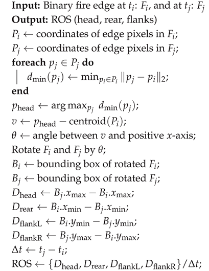
This algorithm computes the head, rear, and flank rates of spread (ROS) of a fire by comparing binary fire-edge maps at two time steps. It identifies the main direction of spread, aligns the fire shapes, and measures directional growth rate in four cardinal directions.
| Algorithm A1: Head of Fire based ROS Calculation |
 |
References
- Pausas, J.G.; Keeley, J.E. Wildfires and global change. Frontiers in Ecology and the Environment 2021, 19, 387–395. [Google Scholar] [CrossRef]
- Hirsch, K.G. Canadian Forest Fire Behavior Prediction (FBP) System: User’s Guide; Number 7, Forestry Canada, Fire Danger Group: Ottawa, Canada, 1996; p. x+–121. [Google Scholar]
- Tymstra, C.; Bryce, R.W.; Wotton, B.M.; Taylor, S.W.; Armitage, O.B. Development and Structure of Prometheus: The Canadian Wildland Fire Growth Simulation Model; Information Report NOR-X-417, Natural Resources Canada, Canadian Forest Service, Northern Forestry Centre: Edmonton, AB, 2010. [Google Scholar]
- Wagner, C.V. Development and structure of the Canadian forest fire weather index system, Number 35. 1987.
- Schroeder, W.; Oliva, P.; Giglio, L.; Csiszar, I.A. The New VIIRS 375 m active fire detection data product: Algorithm description and initial assessment. Remote Sensing of Environment 2014, 143, 85–96. [Google Scholar] [CrossRef]
- Bastarrika, A.; Rodriguez-Montellano, A.; Roteta, E.; Hantson, S.; Franquesa, M.; Torre, L.; Gonzalez-Ibarzabal, J.; Artano, K.; Martinez-Blanco, P.; Mesanza, A.; et al. An automatic procedure for mapping burned areas globally using Sentinel-2 and VIIRS/MODIS active fires in Google Earth Engine. ISPRS Journal of Photogrammetry and Remote Sensing 2024, 218, 232–245. [Google Scholar] [CrossRef]
- Barber, Q.E.; Jain, P.; Whitman, E.; Thompson, D.K.; Guindon, L.; Parks, S.A.; Wang, X.; Hethcoat, M.G.; Parisien, M.A. The Canadian fire spread dataset. Scientific data 2024, 11, 764. [Google Scholar] [CrossRef] [PubMed]
- Zhong, W.; Mei, X.; Niu, F.; Fan, X.; Ou, S.; Zhong, S. Fusing social media, remote sensing, and fire dynamics to track wildland-urban interface fire. Remote Sensing 2023, 15, 3842. [Google Scholar] [CrossRef]
- Andrews, P.L. Current status and future needs of the BehavePlus Fire Modeling System. International Journal of Wildland Fire 2013, 23, 21–33. [Google Scholar] [CrossRef]
- Garcia, T.; Braun, J.; Bryce, R.; Tymstra, C. Smoothing and bootstrapping the PROMETHEUS fire growth model. Environmetrics: The Official Journal of the International Environmetrics Society 2008, 19, 836–848. [Google Scholar] [CrossRef]
- Barber, J.; Bose, C.; Bourlioux, A.; Braun, J.; Brunelle, E.; Garcia, T.; Hillen, T.; Ong, B. Burning issues with PROMETHEUS–the Canadian wildland fire growth simulation model. Canadian Applied Mathematics Quarterly 2008, 16, 337–378. [Google Scholar]
- Silva, J.; Marques, J.; Gonçalves, I.; Brito, R.; Teixeira, S.; Teixeira, J.; Alvelos, F. A systematic review and bibliometric analysis of wildland fire behavior modeling. Fluids 2022, 7, 374. [Google Scholar] [CrossRef]
- Cui, W.; Perera, A.H. What do we know about forest fire size distribution, and why is this knowledge useful for forest management? International Journal of Wildland Fire 2008, 17, 234–244. [Google Scholar] [CrossRef]
- Taylor, S.W.; Woolford, D.G.; Dean, C.; Martell, D.L. Wildfire prediction to inform fire management: statistical science challenges. 2013. [Google Scholar]
- Finney, M.A. An overview of FlamMap fire modeling capabilities. In Proceedings of the In: Andrews, Patricia L.; Butler, Bret W., comps. 2006. Fuels Management-How to Measure Success: Conference Proceedings. 28-30 March 2006; Portland, OR. Proceedings RMRS-P-41; US Department of Agriculture, Forest Service, Rocky Mountain Research Station: Fort Collins, CO, 2006; Vol. 41, pp. 213–220. [Google Scholar]
- USDA Forest Service. Fire Simulation (FSim) Project. 2024. Available online: https://research.fs.usda.gov/firelab/projects/fsim (accessed on 4 December 2024).
- Han, L.; Braun, W. Dionysus: a stochastic fire growth scenario generator. Environmetrics 2014, 25, 431–442. [Google Scholar] [CrossRef]
- Boychuk, D.; Braun, W.J.; Kulperger, R.J.; Krougly, Z.L.; Stanford, D.A. A stochastic forest fire growth model. Environmental and Ecological Statistics 2009, 16, 133–151. [Google Scholar] [CrossRef]
- Braun, W.J.; Woolford, D.G. Assessing a Stochastic Fire Spread Simulator. Journal of Environmental Informatics 2013, 22. [Google Scholar] [CrossRef]
- Jain, P.; Coogan, S.C.; Subramanian, S.G.; Crowley, M.; Taylor, S.; Flannigan, M.D. A review of machine learning applications in wildfire science and management. Environmental Reviews 2020, 28, 478–505. [Google Scholar] [CrossRef]
- Finney, M.A. FARSITE, Fire Area Simulator–model development and evaluation; Number 4, US Department of Agriculture, Forest Service, Rocky Mountain Research Station, 1998. [Google Scholar]
- Freire, J.G.; DaCamara, C.C. Using cellular automata to simulate wildfire propagation and to assist in fire management. Natural hazards and earth system sciences 2019, 19, 169–179. [Google Scholar] [CrossRef]
- Spiller, D.; Thangavel, K.; Sasidharan, S.T.; Amici, S.; Ansalone, L.; Sabatini, R. Wildfire segmentation analysis from edge computing for on-board real-time alerts using hyperspectral imagery. In Proceedings of the 2022 IEEE International Conference on Metrology for Extended Reality, Artificial Intelligence and Neural Engineering (MetroXRAINE); IEEE, 2022; pp. 725–730. [Google Scholar]
- Jonnalagadda, A.V.; Hashim, H.A. SegNet: A segmented deep learning based Convolutional Neural Network approach for drones wildfire detection. Remote Sensing Applications: Society and Environment 2024, 34, 101181. [Google Scholar] [CrossRef]
- Chen, T.H.; Wu, P.H.; Chiou, Y.C. An early fire-detection method based on image processing. In Proceedings of the 2004 International Conference on Image Processing, 2004. ICIP’04; IEEE, 2004; Vol. 3, pp. 1707–1710. [Google Scholar]
- Long, J.; Shelhamer, E.; Darrell, T. Fully convolutional networks for semantic segmentation. In Proceedings of the Proceedings of the IEEE conference on computer vision and pattern recognition; 2015; pp. 3431–3440. [Google Scholar]
- Ronneberger, O.; Fischer, P.; Brox, T. U-net: Convolutional networks for biomedical image segmentation. In Proceedings of the Medical image computing and computer-assisted intervention–MICCAI 2015: 18th international conference, Munich, Germany, 5-9 October 2015; proceedings, part III 18. Springer, 2015; pp. 234–241. [Google Scholar]
- Ghali, R.; Akhloufi, M.A. Deep learning approaches for wildland fires using satellite remote sensing data: Detection, mapping, and prediction. Fire 2023, 6, 192. [Google Scholar] [CrossRef]
- Ghali, R.; Akhloufi, M.A.; Mseddi, W.S. Deep learning and transformer approaches for UAV-based wildfire detection and segmentation. Sensors 2022, 22, 1977. [Google Scholar] [CrossRef]
- Ramos, L.; Casas, E.; Bendek, E.; Romero, C.; Rivas-Echeverría, F. Computer vision for wildfire detection: a critical brief review. Multimedia Tools and Applications 2024, 1–44. [Google Scholar] [CrossRef]
- Kirillov, A.; Mintun, E.; Ravi, N.; Mao, H.; Rolland, C.; Gustafson, L.; Xiao, T.; Whitehead, S.; Berg, A.C.; Lo, W.Y.; et al. Segment Anything. In Proceedings of the 2023 IEEE/CVF International Conference on Computer Vision (ICCV); 2023; pp. 3992–4003. [Google Scholar] [CrossRef]
- Morandini, F.; Silvani, X. Experimental investigation of the physical mechanisms governing the spread of wildfires. International Journal of Wildland Fire 2010, 19, 570–582. [Google Scholar] [CrossRef]
- Viegas, D.X. Slope and wind effects on fire propagation. International Journal of Wildland Fire 2004, 13, 143–156. [Google Scholar] [CrossRef]
- Sharples, J.J.; McRae, R.H.; Wilkes, S.R. Wind–terrain effects on the propagation of wildfires in rugged terrain: fire channelling. International Journal of Wildland Fire 2012, 21, 282–296. [Google Scholar] [CrossRef]
- Thompson, M.P.; Calkin, D.E. Uncertainty and risk in wildland fire management: a review. Journal of environmental management 2011, 92, 1895–1909. [Google Scholar] [CrossRef]
- Linear Mixed-Effects Models: Basic Concepts and Examples. In Mixed-Effects Models in Sand S-PLUS; Springer New York: New York, NY, 2000; pp. 3–56. [CrossRef]
- Finney, M.; Grenfell, I.C.; McHugh, C.W. Modeling containment of large wildfires using generalized linear mixed-model analysis. Forest Science 2009, 55, 249–255. [Google Scholar] [CrossRef]
- Zhang, Z.; Yang, S.; Wang, G.; Wang, W.; Xia, H.; Sun, S.; Guo, F. Evaluation of geographically weighted logistic model and mixed effect model in forest fire prediction in northeast China. Frontiers in Forests and Global Change 2022, 5, 1040408. [Google Scholar] [CrossRef]
- Bugallo, M.; Esteban, M.D.; Marey-Pérez, M.F.; Morales, D. Wildfire prediction using zero-inflated negative binomial mixed models: Application to Spain. Journal of Environmental Management 2023, 328, 116788. [Google Scholar] [CrossRef] [PubMed]
- Anderson, W.R.; Cruz, M.G.; Fernandes, P.M.; McCaw, L.; Vega, J.A.; Bradstock, R.A.; Fogarty, L.; Gould, J.; McCarthy, G.; Marsden-Smedley, J.B.; et al. A generic, empirical-based model for predicting rate of fire spread in shrublands. International Journal of Wildland Fire 2015, 24, 443–460. [Google Scholar] [CrossRef]
- Thompson, J.R.; Wang, X.J.; Braun, W.J. A mouse-model for studying fire spread rates using experimental micro-fires. J. Environ. Stat 2020, 9, 1–19. [Google Scholar]
- Goetz, G.O. A statistical investigation of how slope affects a wildfire’s rate of spread. Master’s thesis, University of British Columbia, 2021. [Google Scholar] [CrossRef]
- Narendra, P.M. A separable median filter for image noise smoothing. IEEE Transactions on Pattern Analysis and Machine Intelligence 1981, 20–29. [Google Scholar] [CrossRef]
- Wagner, C.V. Effect of slope on fire spread rate. 1977. [Google Scholar]
Figure 1.
Scanning Electron Microscope (SEM) image of wax paper employed as a fuel bed analogue in smouldering forest fire simulation.
Figure 1.
Scanning Electron Microscope (SEM) image of wax paper employed as a fuel bed analogue in smouldering forest fire simulation.
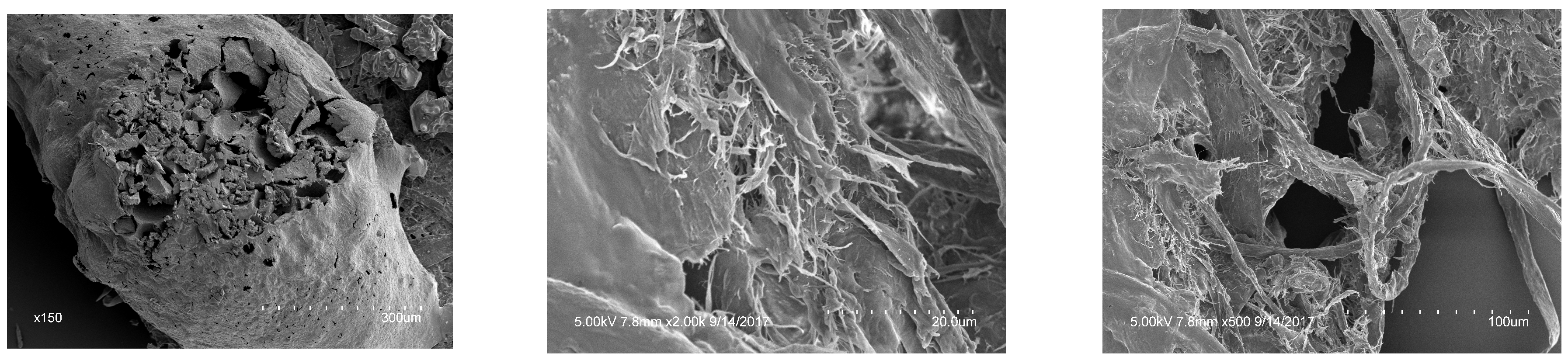
Figure 2.
Fire region segmentation pipeline using the Segment Anything Model (SAM). The process consists of three main stages: Pre-processing including frame extraction, resizing, and ignition coordinate extraction; Segmentation where SAM is applied to isolate fire regions in each frame; and Post-processing which involves smoothing and edge extraction
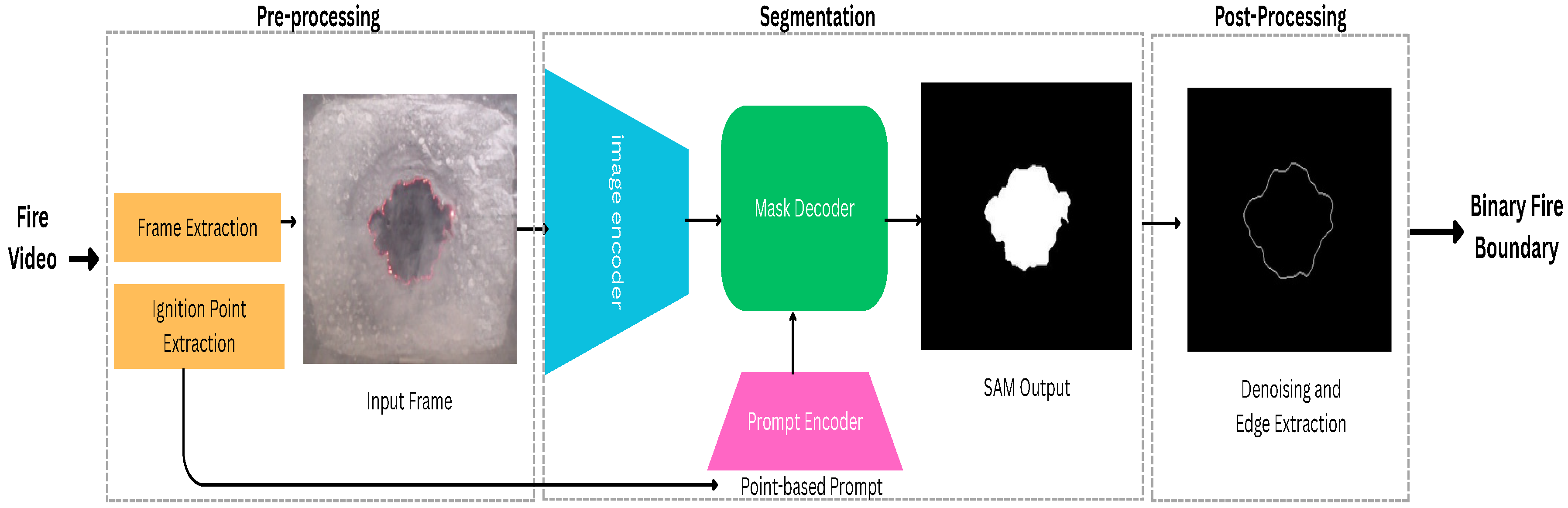
Figure 3.
(a) Evolution of fire boundaries at three time steps, indicated by increasingly darker shades of red. Arrows represent the progression of the fire head between consecutive frames. The observed variation in the direction of the fire head results in two distinct regions of propagation, highlighting spatial variability in fire spread. This directional change leads to shifting definitions of rear and flank zones across time, emphasizing that rear and flank distances are not static but depend on the evolving orientation of the fire head. (b) Our proposed ROS calculation based on bounding boxes around fire boundaries at each time step, providing a consistent, orientation-independent framework for analyzing fire spread.
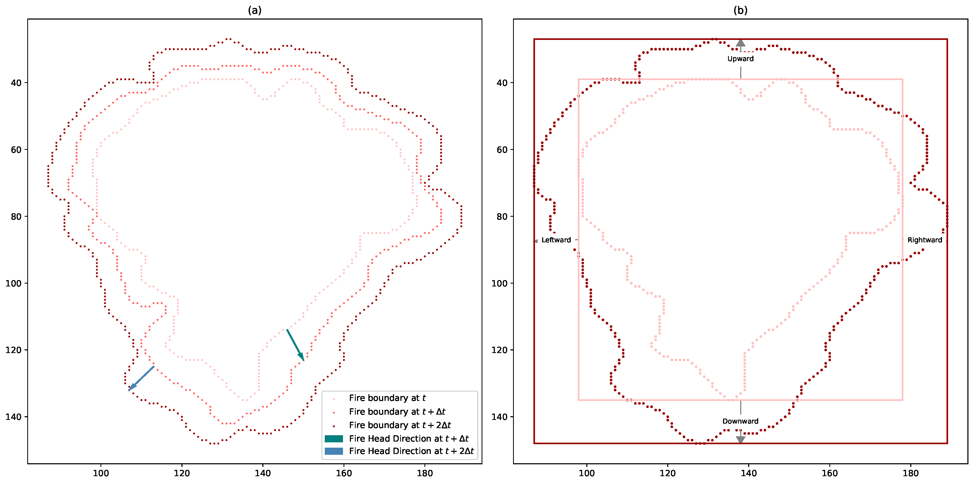
Figure 4.
Diagnostic plots of residuals for the nonlinear regression fitted model of the upslope ROS.
Figure 4.
Diagnostic plots of residuals for the nonlinear regression fitted model of the upslope ROS.
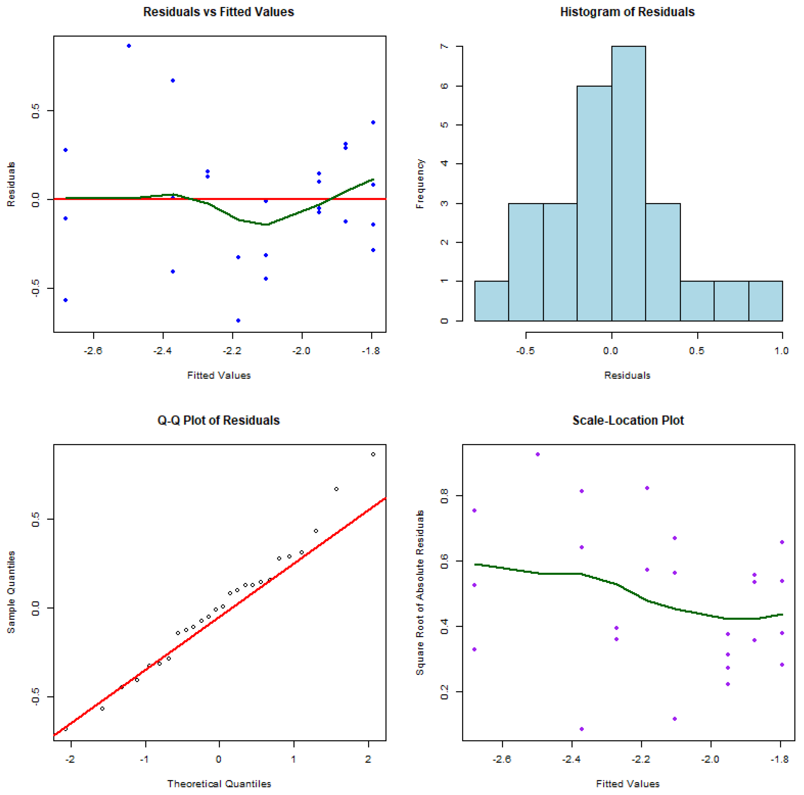
Figure 5.
Comparison of rate of spread of fires on upslope and downslope direction.
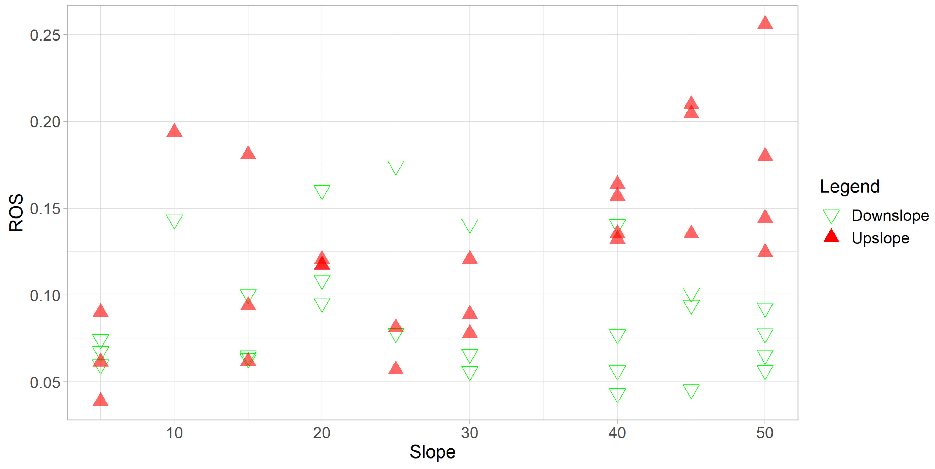
Figure 6.
Spotting for slope degree 25 affecting the downslope rate of spread, upslope is along positive x axis.
Figure 6.
Spotting for slope degree 25 affecting the downslope rate of spread, upslope is along positive x axis.
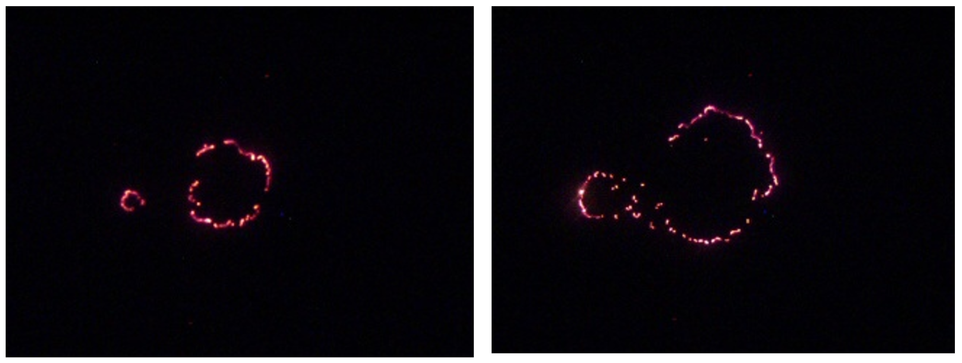

Table 1.
Summary of fixed and random effects on upward ROS from the linear mixed-effects model (250 observations, 10 groups).
Table 1.
Summary of fixed and random effects on upward ROS from the linear mixed-effects model (250 observations, 10 groups).
| Fixed Effects | Estimate | Std. Error | t-value |
|---|---|---|---|
| Intercept | 0.0898 | 0.000 | |
| Soak Time | -0.01352 | 0.1002 | -0.135 |
| Dry Time | 0.01688 | 0.1203 | 0.140 |
| Temperature | 0.09806 | 0.1283 | 0.764 |
| Random Effects | Variance | Std. Dev. | |
| Random Intercept (ID) | 0.08467 | 0.2910 | |
| Residual Variance | 0.90535 | 0.9515 |
Table 2.
Summary of fixed and random effects on downward ROS from the linear mixed-effects model (250 observations, 10 groups).
Table 2.
Summary of fixed and random effects on downward ROS from the linear mixed-effects model (250 observations, 10 groups).
| Fixed Effects | Estimate | Std. Error | t-value |
|---|---|---|---|
| Intercept | 0.0929 | 0.000 | |
| Soak Time | 0.06115 | 0.1038 | 0.589 |
| Dry Time | -0.01550 | 0.1245 | -0.125 |
| Temperature | 0.04586 | 0.1329 | 0.345 |
| Random Effects | Variance | Std. Dev. | |
| Random Intercept (ID) | 0.09204 | 0.3034 | |
| Residual Variance | 0.93725 | 0.9681 |
Table 3.
Parameter estimates for the upslope rate of spread model.
| Parameter | Estimate | Std. Error | t value | p-value |
|---|---|---|---|---|
| d | 0.017386 | 0.001009 | 22.703 | ≤ 2e-16 |
| e | 0.256337 | 0.071923 | 4.319 | 0.000235 |
Table 4.
Parameter estimates for the down slope rate of spread using model (5).
| Parameter | Estimate | Std. Error | t value | p-value |
|---|---|---|---|---|
| d | 0.019594 | 0.001029 | 19.039 | |
| e | -0.017528 | 0.046828 | -0.374 | 0.711 |
Disclaimer/Publisher’s Note: The statements, opinions and data contained in all publications are solely those of the individual author(s) and contributor(s) and not of MDPI and/or the editor(s). MDPI and/or the editor(s) disclaim responsibility for any injury to people or property resulting from any ideas, methods, instructions or products referred to in the content. |
© 2025 by the authors. Licensee MDPI, Basel, Switzerland. This article is an open access article distributed under the terms and conditions of the Creative Commons Attribution (CC BY) license (http://creativecommons.org/licenses/by/4.0/).
Copyright: This open access article is published under a Creative Commons CC BY 4.0 license, which permit the free download, distribution, and reuse, provided that the author and preprint are cited in any reuse.


