

Submitted:
13 September 2023
Posted:
14 September 2023
You are already at the latest version
Abstract
Accurate fuel mapping plays a crucial role in fire detection and management strategies. This paper presents a method for discriminating between wildfire fuel types by exploiting together remote sensing data and Convolutional Neural Networks (CNN). Specially, a CNN-based classification approach that leverages Sentinel-2 imagery is exploited to accurately classify fuel types into seven preliminary main classes (conifers, broadleaf, shrubs, grass, bare soil, urban areas, and water bodies) with an high accuracy of 0.99$\%$. To further refine the fuel mapping results, subclasses were generated from the seven principals by using biomass and bioclimatic maps. These additional maps provide complementary information about vegetation density and climatic conditions, respectively. By incorporating this information, we align our fuel type classification with the widely used Scott/Burgan fuel classification system. This refinement step allows for a more detailed and comprehensive assessment of fuel types, enhancing the accuracy and effectiveness of fire management efforts, which can be utilized by fire management agencies, policymakers, and researchers for improved fire behavior prediction and mitigation practices. The proposed approach presents a valuable tool for enhancing fire management, contributing to more effective wildfire prevention and mitigation efforts.
Keywords:
Fuel Mapping
; Sentinel 2
; CNN Classification
1. Introduction
Accurate and updated information on fuel types and distribution is essential for effective wildfire management [1,2,3], ecosystem planning [4], and their natural resource management [5,6]. Fuel maps, which provide detailed spatial information about vegetation fuel characteristics, play a crucial role in these domains. Traditionally, fuel mapping has relied on ground-based field surveys and visual interpretation of aerial imagery. However, these methods are time-consuming, costly, and limited in coverage. In recent years, Remote Sensing (RS) technology has brought about significant advancements in addressing these limitations. Multispectral and hyperspectral imagery, capable of capturing a wide range of spectral information from the Earth’s surface, have emerged as powerful tools to enhance fuel mapping and related endeavors. Indeed, this spectral information can be used to discriminate between different fuel types based on their unique spectral signatures [7,8,9]. Additionally, Machine learning algorithms, particularly those based on deep learning techniques, have demonstrated exceptional capabilities in extracting complex patterns and relationships from large-scale remote sensing datasets. The combination of remote sensing and machine learning offers numerous advantages for classification tasks providing valuable ancillary information about Earth’s surface proprieties [10,11,12,13]. It enables the generation of fuel maps over large areas in a timely and cost-effective manner, surpassing the limitations of traditional field-based surveys. For instance, I. Chrysafis et al. [14] develop and evaluate random forest classification models using multi-source earth observation data to map fuel types in northeastern Greece. The combination of passive and active Sentinel data, along with topographic variables, improves fuel type classification accuracy. Additionally, Ensley-Field et al.[15] developed a Fuel Model that considers the fuel load from the previous year and utilizes productivity estimates derived from early spring remotely sensed data to predict fuel load at specific locations. D’Este et al. conducted a study (referenced as [16]) on the estimation of fine dead fuel load. They utilized field data, multi-source remote sensing data, and machine learning techniques (Random Forest (RF) and Support Vector Machine (SVM)) to support decision-making and regional wildfire risk management. The results showed that Random Forest performed better in their analysis. Again, the study of Santos et al. [17] aims to improve vegetation representation of fuel load and moisture content in Southern Portugal. Field samples and satellite data from Sentinel-2 were used with the Random Forest classifier for analysis. In recent years, Aragoneses E. and Chuvieco E. [18] developed a methodology for fuel mapping using Sentinel-3 images, vegetation continuity, and biomass data. They compared Support Vector Machine (SVM) and Random Forest (RF) algorithms and found that SVM performed better in their cases. In [19], R.U. Shaik et al. employed an automatic semi-supervised SVM approach to distinguish between 18 different types of wildfire fuel using PRISMA hyperspectral imagery, and resulting in an overall accuracy of 87%. The study proposed by Maniatis Y. et al.[20] develops a fire risk estimation model by using a SVM algorithm, validated by wildfires in 2020 and 2021. Again, a SVM-based method is exploiteed by Garcia M. et al. [21] to classify fuel types by using multispectral data and vertical information provided by the LiDAR, providing an overall accuracy of around 88%. In the woark of Alipour M. et al. [22], a combined approach of Convolutional Neural Network (CNN) and Deep Neural Network (DNN) is developed to provide accurate large-scale fuel estimation. The study mentioned above, published in 2023, represents one of the few available papers in the literature that specifically explores the utilization of Convolutional Neural Networks (CNNs) for fuel mapping. Despite the notable effectiveness of CNNs in remote sensing data analysis across diverse domains, their application to fuel mapping is relatively underexplored. It is worth noting that CNNs have shown promising results in the context of wildfire detection [23,24,25,26,27,28,29].
Thus, the positive outcomes and the limited presence of fuel map applications with Convolutional Neural Networks (CNN) in the existing literature serve as motivation for further exploration and development in this field. In this paper, a novel method that combines remote sensing data and CNNs to discriminate between wildfire fuel types is presented. Specifically, we leverage Sentinel-2 imagery and a CNN-based classification approach to accurately classify fuel types into seven preliminary main classes: conifers, broadleaf, shrubs, grass, bare soil, urban areas, and water bodies. By training the CNN on a large dataset of annotated Sentinel-2 imagery, the model can learn complex patterns and relationships between spectral signatures and fuel types. This enables precise discrimination between different fuel types, facilitating more effective fire detection and management. To refine the fuel mapping results, further subclasses from the seven main classes are generated using Above Ground Biomass (AGB) and Bioclimatic (BC) maps. These additional maps provide valuable information about vegetation density and moisture conditions, respectively. By incorporating these informations, the fuel type classification is aligned with the widely used Scott/Burgan fuel classification system. This refinement step allows for a more detailed and comprehensive assessment of fuel types, enhancing the accuracy and effectiveness of fire detection and management efforts. The proposed approach has the potential to support fire management agencies, policymakers, and researchers in their endeavors to enhance fire prevention and mitigation, ultimately minimizing the impact of wildfires on ecosystems and human populations. The latest advancements in Fuel Map generation have been the focus of this research, demonstrating the capability of CNN-based deep learning techniques in generating precise fuel maps.
This paper is organized as follows. In Section 2, the dataset is described in terms of multispectral Sentinel-2 imagery, areas of interest, ancillary maps (ABG and BC) and Scott/Burgan fuel Model description. The description of the methodology is provided in Section 3, where the CNN-based fuel map classification is described. The results of the training of performance and accuracy are reported in Section 4, while Section 5 deals with the discussion of the numerical findings. Finally, concluding remarks are provided in Section 6.
2. Dataset Definition
This section includes an introduction of the Sentinel-2 multispectral data, a comprehensive exploration of the designated area of interest, an in-depth analysis of the AGB and BC maps and presentation of Scott/Burgan Fuel Type.
2.1. Sentinel Data
This section provides a description of the Sentinel multispectral data used for training and validating the CNN model. In our study, spectral images from Sentinel-2 acquired on July 17, 2022 were utilized as the primary dataset for training the Convolutional Neural Network (CNN). The Sentinel-2 satellite sensor captures images in multiple spectral bands, which provide valuable information about Earth’s surface. The Sentinel-2 mission, launched by the European Space Agency (ESA), aims to provide global and systematic observations of the Earth’s land and coastal areas. It consists of two identical satellites, Sentinel-2A and Sentinel-2B, which together cover the entire Earth’s landmass every 5 days. The satellites acquire high-resolution imagery in 13 spectral bands with spatial resolution of 10, 20 and 60 meters, enabling the monitoring of land cover, vegetation dynamics, and environmental changes. For our analysis, all the sensor bands were resized to a spatial resolution of 10 meters. To further improve classification, several vegetation indices were calculated from the Sentinel-2 bands and added to the spectrum dataset: the Normalized Difference Vegetation Index (NDVI), Enhanced Vegetation Index (EVI) and Normalized Difference Water Index (NDWI) widely used to assess vegetation health and density, reported in Table 1.
2.2. Area of Interest
As shown in Figure 1, the focus of this study centers around Sardegna, an island positioned in the southern region of Italy and recognized as the second-largest landmass in the Mediterranean Sea. Specifically, Sardegna has gained notoriety for the frequent prevalence of wildfires. Over the preceding decade, this island has witnessed an annual average of 1008 fire incidents, constituting a significant 20% of the overall national tally [30]. The occurrence and magnitude of these fires in Sardegna are greatly influenced by the island’s distinctive climatic conditions. The area is characterized by gusty winds, intermittently wet winters, and scorching, sun-drenched summers. The temperature fluctuations are noteworthy, ranging from 10°C during the winter months of January and February to a balmy 24-25°C during the summer period encompassing July and August [31]. To assess the Fuel Map under high-risk fire probability conditions and during periods of significantly increased fuel load, a satellite image captured by the Sentinel-2 on July 17, 2022, during the summer season, was selected for analysis. The particular area selected and situated east of Cagliari, consists of an expansive forested landscape that traverses undulating terrain, reaching altitudes of approximately 800 meters, encompassing a total land area of 32 . Then, the reference data were obtained through a visual inspection of the false RGB image derived from the Sentinel-2 image of the region of interest. The number of labelled pixels for each class are reported Table 2.
One can notice that the higher frequency of the Water classes compared to the others can be attributed to its ease of identification and widespread presence within the examined image. These favorable conditions facilitated the labeling process by allowing for a larger number of instances to be accurately labeled without the risk of incorporating impure pixels. Conversely, the remaining classes exhibited increasingly intricate discrimination challenges. Despite their substantial representation in the image, a more extensive and demanding exploration was required. The imperative to collect pure pixels required more rigorous selection, resulting in a sample set that was small but definitely pure, and thus fully characteristic of the respective classes. This problem was particularly pronounced for the Bare Grounds and Grass classes, where the combination of a limited amount of samples and the inherent complexity of assessing their purity led to a deliberate preference for a smaller sample set. However, these samples remained unequivocally representative of the reference class despite their small number.
2.3. Ancillary Maps
This section provides a detailed overview and descrition of how the AGB and BC ancillary maps are carried out, highlighting their crucial contribution in enhancing the classification process. Indeed, our preliminary land cover classification relies on a limited number of classes, which may not capture the fine-scale variability within a given region. Thus, to address this limitation, an approach that utilizes additional data layers is exploited, specifically AGB and BC maps, to generate a more detailed subclassification scheme from a primary land cover classification obtained through Convolutional Neural Networks (CNNs). Then the final subclassification is aligbned with the widely accepted Scott/Burgan fuel classification system.
- The Aboveground Biomass Map represents the total mass of living vegetation per unit area, typically expressed in metric tons per hectare (unit: tons/ha). The AGB map used in this study was obtained from the European Space Agency’s (ESA’s) Climate Change Initiative (CCI) programme [32], that is an ESA project to provide long-term, high-quality climate data records to support climate change research and related applications (the AGB map can be downloaded for free at link: https://data.ceda.ac.uk/neodc/esacci/biomass/data/agb/maps, accessed on 25 May 2023). The AGB map of ESA exhibites a continuous range of values, however, in this work, the biomass values are normalized as percentages relative to the maximum value. Subsequently, the AGB map is divided into three macrogroups based on the following percentage thresholds: the first group includes all values below 40%, the second group encompassed values between 40% and 70%, and the third group included values exceeding 70%. This is done to facilitate analysis and align with the Scott/Burgan fuel type classification. Indeed, this approach allowed us to establish a direct correlation between the biomass percentages and the Scott/Burgan fuel type classification, specifically the distinction between low, medium, and high forest density. Furthermore, due to the initial resolution of the raster being 100 meters, it was imperative to rescale the map to a finer resolution of 10 meters. This resampling process was performed using QGIS software, ensuring the preservation of relevant spatial information and maintaining data integrity throughout the analysis. The post-proccessed AGB map is reported in the left side of Figure 2, where the 3 main classes abovementioned are reported. As expected from RGB image in Figure 1, a predominant representation of classes below the 70 percent threshold is observed, indicating a dense vegetation cover exclusively in the most remote regions of the study area, specifically the peaks located within the inner mountains. On the contrary, the remaining portion of the region of interest predominantly consists of agricultural fields, grasses or sparsely forested areas. This finding emphasizes the crucial importance of incorporating the use of this map, as it clearly reveals the pronounced disparity in land cover composition and illuminates the unique ecological features present in the study area.
-
The Climate Map is derived from the BC map of Sardinia that was developed through a collaboration among several institutions:
- –
- ARPAS - Regional Agency for Environmental Protection of Sardinia (Agenzia Regionale per la Protezione dell’Ambiente della Sardegna) - Meteoclimatic Department, Sassari: ARPAS is the regional agency responsible for environmental protection in Sardinia. Their Meteoclimatic Department contributed to data collection.
- –
- University of Sassari, Department of Natural and Territorial Sciences, Sassari: The Department of Natural and Territorial Sciences at the University of Sassari provided scientific expertise and knowledge in the field of environmental sciences.
- –
- University of Basilicata, School of Agricultural, Forestry, Food, and Environmental Sciences, Potenza: The University of Basilicata contributed with their expertise in the fields of agricultural, forestry, food, and environmental sciences.
Through the synergy among these institutions, it was possible to create the BC map of Sardinia, an important tool for understanding and studying the climates and biodiversity of the island [33]. The BC map represents the final stage of processing, achieved through the overlay of multiple layers such as Macrobioclimates, Phytoclimatic Plans, Ombrothermal Index, and Continentality Index. This intricate overlay generates a new layer that encompasses diverse combinations of bioclimatic values for each polygon. The resulting BC map comprises 43 classes of Isobioclimates, reflecting the detailed classification approach employed to capture the intricate characteristics of Sardinia’s terrain. These 43 classes span a range of climate levels, encompassing dry, subhumid, humid, and hyperhumid conditions. Therefore, our focus lies on the subset of classes among the 43 available, specifically those that belong to one of the four predefined categories. By doing so, we generate a simplified map comprising two distinct macrogroups, categorized as follows: 1) "Dry," encompassing all the dry classes, and 2) "Humid," encompassing the remaining classes (subhumid, humid, and hyperhumid). The climate map carried out with this approach is reported on the right side of Figure 2.Figure 2. Ancillary Maps: (on left side) the Above-Ground Biomass derived from ESACCI biomass map, and (on the rigth side) the climatic zone map derived by the Sardegna Bioclimatic map, see text.Figure 2. Ancillary Maps: (on left side) the Above-Ground Biomass derived from ESACCI biomass map, and (on the rigth side) the climatic zone map derived by the Sardegna Bioclimatic map, see text.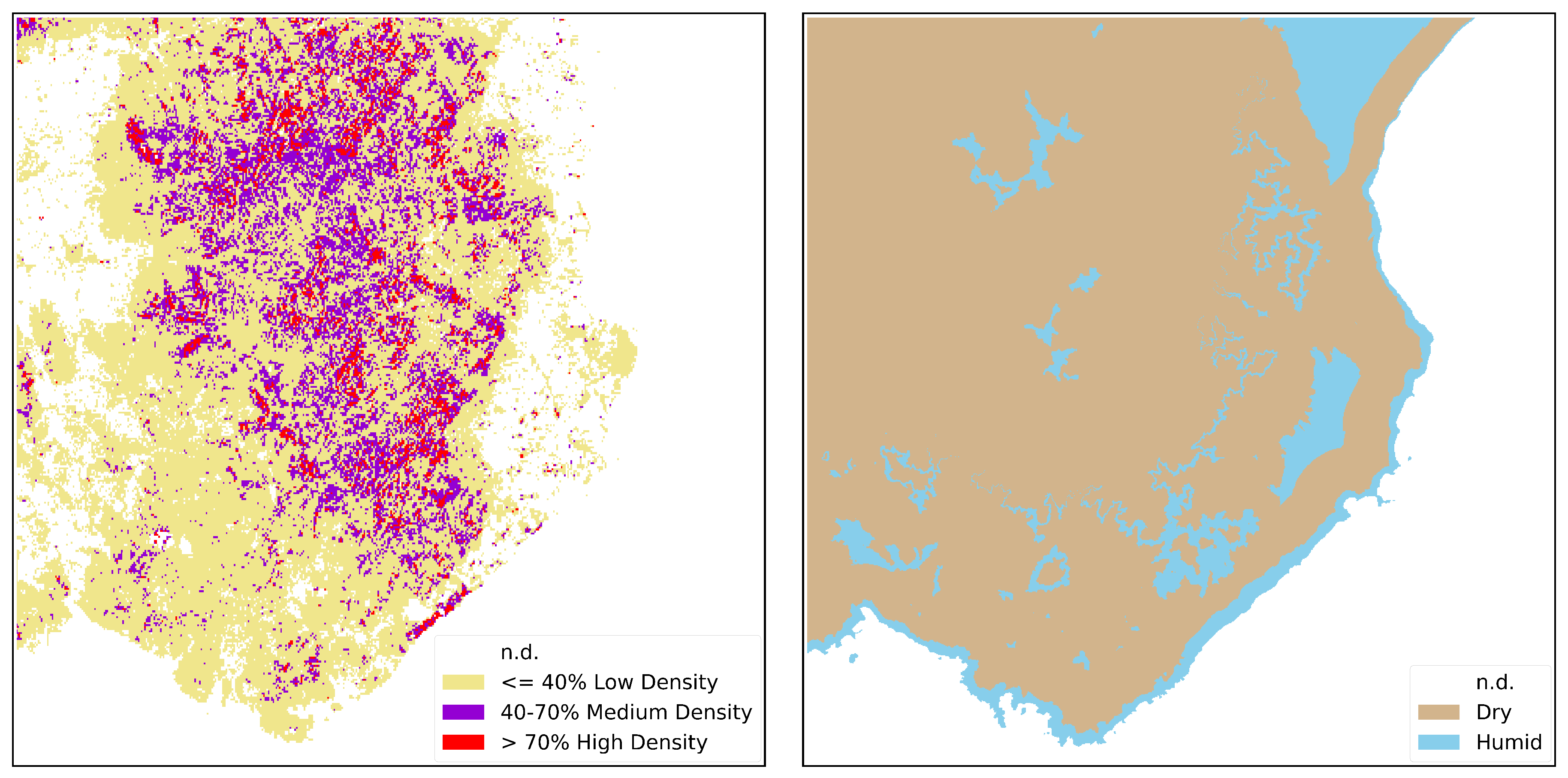
By considering all the possible combinations between the two maps, six distinct classes are obtained, as illustrated in Figure 3. These classes are categorized as follows: dry-low, dry-medium, dry-high, humid-low, humid-medium, and humid-high. The integration of these distinct classes provides a comprehensive representation of the varying levels of dryness and density vegetation across the studied area. The resulted ancillary map is called Biomass-Dryness map (BD).
2.4. Scott-Burgan Fuel Model
Standard Fire Behavior Fuel Models (SFBFM) developed by Scott and Burgan [34] provide a systematic and standardized approach to characterizing vegetation and fuel properties, allowing fire analysts to assess and predict fire behavior under different fuel conditions. The SFBFM system serves as a critical tool in fire management decision-making processes. The SFBFM comprises a structured set of 45 distinct fuel models, out of which 5 are non-burnable types, namely Urban, Snow/Ice, Agricultural, Open Water, and Bare Ground. The remaining fuel models within the system are burnable and represent various vegetation and fuel characteristics. These models are carefully designed to capture the diverse range of fuel properties encountered in different fire-prone environments. The SFBFM system provides a comprehensive representation of fuel characteristics by considering factors such as fuel loadings, fuel particle sizes, and moisture content. Each fuel model is assigned a unique numeric code and accompanied by a descriptive name, facilitating standardized communication and data exchange among fire management professionals, a schematic description is reported in Table 3.
3. Method
The presented approach involves a two-step process. Firstly, a CNN-based classification is exploited to generate a primary land cover classification. This initial classification scheme provides a broad characterization of the different land cover classes (reported in Table 2) and exploits the Sentinel-2 multispectral images. Subsequently, the BD map is integrated to refine the primary classification adapting them according to the classification of fuel types defined by Scott/Burgan.
3.1. CNN Architecture
The CNN convolutional neural network model is implemented in Python by using TensorFlow. The model is designed for multi-class classification tasks and it consists of several layers of one-dimensional convolutional, pooling, and fully connected nodes, as schematized in Figure 4. The CNN inputs consist of an array with a predetermined length of 16 elements, encompassing the 13 bands of the Sentinel-2 image as well as the 3 indices provided in Table 1. The first hidden layer of the model is a convolutional layer with 224 filters and kernel size 3, with the kernel regularizer L2 and regularization coefficient equal to 1e-5, and ReLU activation function. The output of this layer is passed through a max pooling layer that reduces the dimension of the feature map by a factor of 2. The second layer of the model is another convolutional layer with 112 filters and kernel size 3, with the kernel regularizer L2 and regularization coefficient equal to 1e-5, and ReLU activation function. Again, the output of this layer is passed through a max pooling layer that reduces the dimension of the feature map by a factor of 2. The pooled feature map is flattened in a vector of length 336 and passed through two fully connected layers. The first fully connected layer has 224 units with ReLU activation function, and the second fully connected layer consists of 128 units with ReLU activation function. Finally, the output is passed through a softmax activation function with 7 classes to produce the predicted class probabilities. The model is trained using the Adam optimizer with a learning rate of "learnrate". The loss function used is categorical cross-entropy, and the model is evaluated based on the accuracy metric. The dropout technique with rate "drop" is also used to regularize the fully connected layers. The whole network has been implemented using Python and Keras.
It is important to note that after performing the land cover classification using CNN, the classes Bare Soil, Urban and Water are not taken into account when generating the fuel type map, as they fall directly into the Non-burnable category. Therefore, from this point on, only the other classes will be considered in the methodology.
3.2. CNN-based Unmixing
This methodology exploits the inherent probabilistic features of CNN results to effectively deal with pixel confusion in scenarios where multiple classes coexist. Specifically, when the CNN model demonstrates satisfactory performance in pure pixel recognition, pixel confusion mainly results from impure pixels that include mixed features. For instance, when a pixel contains both grass and shrubs, the CNN output may exhibit a 50/50 balanced probability distribution. Importantly, this distribution reflects the presence of both classes rather than being an error in the CNN prediction. Leveraging this concept, multiple class assignments can be intelligently carried out from CNN prediction. In particular, the main objective is to identify the classes related to the GS and TU fuel models of the Scott/Burgan Fuel Model, specifically targeting the Grass-Shrub, Timber-Shrub, and Timber-Grass-Shrub classes (in this work, the term "Timber" includes both Broadleaf and Coniferous classes).
In the practical implementation, following the prediction of the probability for each pixel within the area of interest, a subsequent pixel-level analysis is conducted. The following steps describe the algorithm that is performed for each pixel prediction:
- If the maximum probability is below 60%, proceed to the next step. Otherwise, retain the original class assignment.
- Check the second maximum probability. If it exceeds 20% and the third maximum probability is below 20%, assign the pixel to both the first and second classes.
- If the third maximum probability is also above 20%, assign the pixel to all three classes.
- If the first class probability is below 60% and all other probabilities are below 20%, retain the pixel’s original class assignment.
The classes obtained after applying CNN-based classification and unmixing are as follows: Broadleaf, Conifer, Shrub, Grass, Grass-Shrub, Timber-Shrub (Broadleaf-Shrub and Conifer-Shrub), and Timber-Shrub-Grass (Broadleaf-Shrub-Grass and Conifer-Shrub-Grass).
3.3. Fuel Map Adaptation
To enhance the level of detail in the fuel map, the land cover classification obtained with the procedure aforementioned and the BD map were cross-referenced, resulting in a total of 42 classes. Specifically, this includes the 7 classes from the classification combined with the 6 classes from the BD map, which were subsequently associated with corresponding fuel models from the Scott/Burgan system, as reported in Table 4. The resultant adaptation affords a comprehensive representation of fuel characteristics that serves as a valuable resource for decision-makers involved in land management and fire risk assessment. Armed with this comprehensive representation of fuel characteristics, authorities and stakeholders can make well-informed decisions regarding wildfire prevention strategies, resource allocation, and emergency response planning. The detailed fuel map empowers them to identify high-risk areas, prioritize mitigation efforts, and enhance the overall resilience of the landscape against fire hazards.
4. Results
This section presents the performances of CNN model in terms of accuracy, validation and comparison with RF and SVM, as well as the final classification of the Fuel Map aligned with the Scott/Burgan fuel model.
4.1. Performances of CNN Classification
The training and testing phases utilized the dataset derived from visual inspection, while the validation involved the entire image and cross-referencing with external source maps as ground truth, ensuring a robust assessment of the model’s performance. Moreover, a comparison is conducted with RF and SVM to underscore the potential of the CNN-based fuel map generator.
4.1.1. Model Accuracy
In the practical implementation, the dataset reported in Table 2 was divided into training and test subsets, with a split ratio of 70% and 30% respectively. The model performances were conducted using a personal computer equipped with a 12th Generation Intel Core i7-12700H 2.70 GHz CPU, 12 GB of RAM, and an NVIDIA GeForce RTX 3080 Ti GPU with 16 GB of dedicated RAM. The results of the CNN model training and testing in terms of Precision (0.99), Recall (0.99), and F1 (0.99) score are exceptionally high, demonstrating that the network has been effectively trained to accurately identify pure pixels. In Figure 5 one can appreciate the segmentation results over the region of interest on the left side, and the confusion matrix on the right side. One can notice that the Not Burnable classes (Bare Soil, Urban, and Water) are perfectly recognized, while a slight degree of confusion is observed among the other classes due to increasing spectral similarity.
4.1.2. Validation on Sardegna
While the training and testing phases were conducted using the dataset obtained through visual inspection (see Table 2), the validation process involved the entire image. In this validation step, the predictions were compared and validated against external source maps, recognized as ground truth, to evaluate the model’s reliability in classifying pixels beyond the original dataset. To achieve this, a set of four carefully selected validation maps was utilized, each distinctly representing specific classes: 1) Land Cover (LC) 2021, provided by ISPRA ("Istituto Superiore per la Protezione e la Ricerca Ambientale"), represents the bio-physical coverage of the Earth’s surface, including Broadleaf, Conifer, Shrub, and Grass classes (https://www.isprambiente.gov.it/it); 2) ESA WorldCover (WC) 2021 includes 11 generic classes representing different land surface types, including Tree cover, Shrubland, Grassland, and Cropland (https://worldcover2021.esa.int); 3) Forest Type product (FTY) is a part of the European Environment Agency (EEA) Copernicus Land Monitoring Service, and it provides a forest classification with 3 thematic classes: non-forest areas, broadleaved forest, and coniferous forest (https://land.copernicus.eu/pan-european/high-resolution-layers/forests/forest-type-1/status-maps/forest-type-2018); 4) Grassland (GRA) 2018 is also developed under the EEA Copernicus Land Monitoring Service, and it offers a basic land cover classification with 2 thematic classes: grassland and non-grassland (https://land.copernicus.eu/pan-european/high-resolution-layers/grassland/status-maps/grassland-2018). This deliberate selection enabled a thorough evaluation of the model’s performance across diverse class categories, offering valuable insights into its generalization capabilities and adaptability in various scenarios. Notably, the model achieves an impressive accuracy of 99% for the Broadleaf class, indicating its exceptional ability to accurately classify the majority of pixels belonging to this category. The Conifer class also performs well with a respectable accuracy of 79%, showcasing its capability to effectively classify Conifer-related pixels. Though slightly lower, the model still demonstrates solid performances for the Shrub and Grass classes, achieving accuracies of 76% and 84%, respectively. The remaining classes are regarded as non-burnable and thus were not taken into account during the validation phase.
4.1.3. Comparison with RF and SVM
The RF model was implemented using the "RandomForestRegressor" function from the "catboost" library in Python. The model was set with 500 boosting iterations and a maximum tree depth of 5 to avoid overfitting. The ’MultiRMSE’ loss function was employed for optimization, and a learning rate of 0.1 was utilized to control the step size during training. The computations were performed on a GPU, and early stopping with 500 rounds was applied to prevent overfitting.
Instead, the SVM model was implemented using the "SVC" function from the "scikit-learn" library in Python. For the classification task, the radial basis function ("rbf") was chosen as the kernel function. To ensure repeatability, a random seed of 0 () was set. Additionally, the model was configured to provide class probabilities using the probability parameter set to True. A gamma value of 100 was employed for model tuning, which influences the flexibility of the decision boundary.
The results presented in Table 5 display the performances of all three models in terms of accuracy, recall, and F1 scores. The results suggest that all three models exhibit similar performances, showing only minor variations. However, it is noteworthy that the RF and CNN models outperform the SVM model by a small margin.
Consequently, in Table 6 the Support Vector Machine (SVM) is disregarded and the results are reported only for CNN and RF. The results, once again, demonstrate relatively similar performances among the models. However, the Convolutional Neural Network (CNN) does exhibit a slight advantage, particularly in the classification of Coniferous land cover. The CNN achieves an accuracy of 0.78%, while the RF achieves an accuracy of 0.70%.
Despite the similarities in overall performance, this advantage of the CNN model in classifying Coniferous regions highlights its potential as a more adept solution for tasks that require discerning subtle and complex patterns in land cover data. These findings further emphasize the CNN’s proficiency in image analysis and its applicability in geospatial studies and remote sensing applications.
4.2. Fuel Map Generation
By utilizing a CNN-based classification approach with Sentinel-2 imagery, the fuel types are precisely categorized into seven primary classes. Subsequently, subclasses are derived by integrating the BD map, which effectively aligns the classification with the Scott/Burgan fuel system. Considering the high accuracy observed in the proposed classification and the validation of the ancillary maps as ground truth, the resulting fuel map is expected to exhibit similar levels of accuracy. This map, reported in Figure 6, is a product of the integration and cross-referencing of these complementary maps, ensuring a robust and reliable classification outcome.
5. Discussion
This research was driven by the need to advancing land cover classification methodologies, fuel mapping techniques, and remote sensing applications. In response to this demand, the research introduces a CNN-based Fuel Map generator utilizing Sentinel-2A satellite images.
The presented results provide valuable insights into the performance and potential applications of the CNN model for land cover classification and fuel map generation. The CNN model demonstrates exceptional accuracy (0.99%), recall (0.99%), and F1 scores (0.99%), indicating its proficiency in accurately identifying pure pixels. One can notice that the Not Burnable classes (Bare Soil, Urban, and Water) are accurately recognized by the model, as these classes possess distinct spectral patterns that facilitate reliable identification. However, there is a slight degree of confusion observed among the other classes, mainly attributed to the increasing spectral similarity, which makes accurate classification more challenging. It is worth mentioning an intriguing observation, although somewhat unrelated to the main focus, where the model successfully classifies some vessels located off the East Coast as "urban," even when they were barely visible to the naked eye. This demonstration of the model’s overall capability and accuracy is noteworthy and piques further interest in its potential applications. These results underscore the strength and promise of the CNN model in advancing land cover mapping and monitoring, making it a valuable tool for geospatial studies and remote sensing applications.
In the validation phase, the CNN model’s robustness is evaluated by comparing its predictions against external source maps as ground truth. The validation results demonstrate high accuracy, particularly in distinguishing the Broadleaf (0.99%) and Grass (0.84%) classes. The model’s ability to accurately classify these classes can significantly contribute to land cover mapping and monitoring applications. However, the slightly lower accuracies for the Shrub (0.76%) and Conifer (0.78%) classes suggest that further refinement or data augmentation may be beneficial for improving their performance. It is worth noting that the variations in accuracy across classes could be due to the inherent differences in features and characteristics among these land cover categories. Additionally, other factors like data imbalance, the availability of training samples, and class complexity might influence the results. Overall, these results suggest that the CNN model performs well in classifying land cover types, with particularly outstanding performance for the Broadleaf class. These high validation accuracy values provide evidence of the model’s ability to generalize well beyond the original training dataset. This generalization capability is crucial for real-world applications, where the model is expected to accurately classify land cover in diverse and previously unseen regions.
The comparison with RF and SVM models reveals that all three models exhibit similar performances with minor variations. While the SVM model could be disregarded due to producing slightly inferior results, the CNN and RF models stand out as strong contenders. In particular, the CNN model shows a slight advantage in classifying Coniferous land cover, which underscores its potential in discerning subtle and complex patterns in land cover data. The CNN’s proficiency in image analysis and geospatial studies opens new possibilities for remote sensing applications. The CNN achieves an impressive accuracy of 0.78 for Coniferous regions, while the Random Forest (RF) model falls short with an accuracy of 0.70 for the same category.
The fuel map generation process aligns the land cover classification with the wellknown Scott/Burgan fuel system, effectively categorizing fuel types into seven primary classes and derived subclasses. By integrating AGB and BC maps, the resulting fuel map exhibits high accuracy. This accuracy is crucial as it can greatly contribute to fire risk assessment and management efforts. The accurate and detailed fuel map enables firefighters, land managers, and policymakers to develop effective strategies for wildfire suppression and sustainable land use practices. Moreover, the fuel map finds applications beyond fire management, supporting ecosystem restoration, habitat conservation, and resource management initiatives. Overall, the research emphasizes the vital role of the fuel map in enhancing wildfire management and promoting ecological resilience.
The method’s limitation could its reliance on external biomass and climate maps as fundamental inputs for generating the final Fuel Map classification. Moreover, the availability of such maps may be limited across different regions. The availability of these maps may vary across different regions and could pose challenges for areas where such data is scarce or unavailable.
To address this, future research could focus on developing an autonomous AGB estimation system solely based on Sentinel-2A spectral images, eliminating the need for external maps. However, this poses a complex challenge, requiring a deep understanding of spectral signals and precise model calibration and validation with ground reference data. Thus, the AGB map provided by ESA can serve as the ground reference label for training the Convolutional Neural Network (CNN). This method could offers promising opportunities but also faces some potential limitations. For instance, the accuracy of the ESA AGB map itself is crucial, such as the spatial and temporal alignment of ESA’s AGBs with Sentinel-2A images, as any errors or uncertainties in this map can directly impact the reliability of the CNN’s predictions. Moreover, the limited coverage of the ESA AGB map may pose challenges, particularly in remote or inaccessible areas, where biomass estimates might be unavailable. It is essential to ensure a comprehensive and representative training dataset to account for different land cover types and biomass levels to avoid biases in the model. In conclusion, while the proposed CNN-based method using the ESA AGB map as a label offers exciting possibilities for autonomous fuel mapping, it is crucial to address the potential limitations mentioned above to ensure the method’s accuracy and practicality in real-world applications. By mitigating these challenges, the proposed approach can make valuable contributions to land cover classification and biomass estimation, supporting various fields such as environmental management, disaster response, and resource conservation.
6. Conclusions
In conclusion, the CNN model’s exceptional performance in land cover classification, especially in distinguishing the Broadleaf and Conifer classes, showcases its potential for land cover mapping and monitoring tasks. The model’s proficiency in analyzing complex spatial patterns positions it as a promising tool for remote sensing applications. The generated fuel map aligns with the Scott/Burgan fuel system, presenting a valuable asset in wildfire risk assessment and mitigation. Further research and refinement may lead to even more accurate and versatile applications of the CNN model in geospatial studies and remote sensing. The demonstrated capabilities highlight the importance of utilizing advanced machine learning techniques to address complex environmental challenges and support effective land management strategies. Fuel mapping is essential for wildfire management and prevention. Accurate fuel mapping helps identify areas at higher risk of wildfires, enabling authorities to implement proactive measures to mitigate fire hazards and improve firefighting strategies. By leveraging CNN models for land cover classification, this research showcases the potential of artificial intelligence and machine learning techniques in remote sensing applications. It paves the way for more efficient and automated analysis of large-scale satellite imagery, benefiting various fields such as agriculture, forestry, disaster monitoring, and environmental studies. The results of this study could be expanded in future works both considering bigger and diver training datasets and more complex neural networks capable of carrying out an ABG prediction.
Author Contributions
Conceptualization, A.C. and G.L.; methodology, A.C.and G.L; software, A.C and D.S.; validation, A.C.; formal analysis, A.C.; investigation, A.C.; resources, G.L.; data curation, A.C.; writing—original draft preparation, A.C.; writing—review and editing, A.C., D.S. and G.L.; visualization, A.C.; supervision, D.S. and G.L.
Funding
This research received no external funding.
Institutional Review Board Statement
Not applicable.
Informed Consent Statement
Not applicable.
Acknowledgments
The subject of this paper has been motivated by the research activity carried out in the framework of the FirEUrisk project.
Conflicts of Interest
The authors declare no conflict of interest.
References
- McCaffrey, S. Thinking of wildfire as a natural hazard. Society and Natural Resources 2004, 17, 509–516. [Google Scholar] [CrossRef]
- Bowman, D.M.; Balch, J.; Artaxo, P.; Bond, W.J.; Cochrane, M.A.; D’antonio, C.M.; DeFries, R.; Johnston, F.H.; Keeley, J.E.; Krawchuk, M.A.; others. The human dimension of fire regimes on Earth. Journal of biogeography 2011, 38, 2223–2236. [Google Scholar] [CrossRef] [PubMed]
- Knorr, W.; Arneth, A.; Jiang, L. Demographic controls of future global fire risk. Nature Climate Change 2016, 6, 781–785. [Google Scholar] [CrossRef]
- Pausas, J.G.; Keeley, J.E. A burning story: the role of fire in the history of life. BioScience 2009, 59, 593–601. [Google Scholar] [CrossRef]
- Eva, H.; Lambin, E.F. Fires and land-cover change in the tropics: a remote sensing analysis at the landscape scale. Journal of Biogeography 2000, 27, 765–776. [Google Scholar] [CrossRef]
- Cano-Crespo, A.; Oliveira, P.J.; Boit, A.; Cardoso, M.; Thonicke, K. Forest edge burning in the Brazilian Amazon promoted by escaping fires from managed pastures. Journal of Geophysical Research: Biogeosciences 2015, 120, 2095–2107. [Google Scholar] [CrossRef]
- Shaik, R.U.; Periasamy, S.; Zeng, W. Potential Assessment of PRISMA Hyperspectral Imagery for Remote Sensing Applications. Remote Sensing 2023, 15. [Google Scholar] [CrossRef]
- Congalton, R.G. Remote Sensing: An Overview. GIScience & Remote Sensing 2010, 47, 443–459. [Google Scholar] [CrossRef]
- Navalgund, R.R.; Jayaraman, V.; Roy, P. Remote sensing applications: An overview. current science 2007, 1747–1766. [Google Scholar]
- Maxwell, A.E.; Warner, T.A.; Fang, F. Implementation of machine-learning classification in remote sensing: an applied review. International Journal of Remote Sensing 2018, 39, 2784–2817. [Google Scholar] [CrossRef]
- Camps-Valls, G. Machine learning in remote sensing data processing 2009. pp. 1–6. [CrossRef]
- Lary, D.J.; Alavi, A.H.; Gandomi, A.H.; Walker, A.L. Machine learning in geosciences and remote sensing. Geoscience Frontiers 2016, 7, 3–10, Special Issue: Progress of Machine Learning in Geosciences. [Google Scholar] [CrossRef]
- Scheunders, P.; Tuia, D.; Moser, G., Contributions of machine learning to remote sensing data analysis. In Data processing and analysis methodology; Liang, S., Ed.; Comprehensive remote sensing, Elsevier: Netherlands, 2018; pp. 199–243. [CrossRef]
- Chrysafis, I.; Damianidis, C.; Giannakopoulos, V.; Mitsopoulos, I.; Dokas, I.M.; Mallinis, G. Vegetation Fuel Mapping at Regional Scale Using Sentinel-1, Sentinel-2, and DEM Derivatives—The Case of the Region of East Macedonia and Thrace, Greece. Remote Sensing 2023, 15. [Google Scholar] [CrossRef]
- Ensley-Field, M.; Shriver, R.K.; Law, S.; Adler, P.B. Combining Field Observations and Remote Sensing to Forecast Fine Fuel Loads. Rangeland Ecology & Management, 2023. [Google Scholar] [CrossRef]
- D’Este, M.; Elia, M.; Giannico, V.; Spano, G.; Lafortezza, R.; Sanesi, G. Machine Learning Techniques for Fine Dead Fuel Load Estimation Using Multi-Source Remote Sensing Data. Remote Sensing 2021, 13. [Google Scholar] [CrossRef]
- Santos, F.L.; Couto, F.T.; Dias, S.S.; de Almeida Ribeiro, N.; Salgado, R. Vegetation fuel characterization using machine learning approach over southern Portugal. Remote Sensing Applications: Society and Environment 2023, 32, 101017. [Google Scholar] [CrossRef]
- Aragoneses, E.; Chuvieco, E. Generation and Mapping of Fuel Types for Fire Risk Assessment. Fire 2021, 4. [Google Scholar] [CrossRef]
- Shaik, R.U.; Laneve, G.; Fusilli, L. An automatic procedure for forest fire fuel mapping using hyperspectral (PRISMA) imagery: A semi-supervised classification approach. Remote Sensing 2022, 14, 1264. [Google Scholar] [CrossRef]
- Maniatis, Y.; Doganis, A.; Chatzigeorgiadis, M. Fire Risk Probability Mapping Using Machine Learning Tools and Multi-Criteria Decision Analysis in the GIS Environment: A Case Study in the National Park Forest Dadia-Lefkimi-Soufli, Greece. Applied Sciences 2022, 12. [Google Scholar] [CrossRef]
- García, M.; Riaño, D.; Chuvieco, E.; Salas, J.; Danson, F.M. Multispectral and LiDAR data fusion for fuel type mapping using Support Vector Machine and decision rules. Remote Sensing of Environment 2011, 115, 1369–1379. [Google Scholar] [CrossRef]
- Alipour, M.; La Puma, I.; Picotte, J.; Shamsaei, K.; Rowell, E.; Watts, A.; Kosovic, B.; Ebrahimian, H.; Taciroglu, E. A Multimodal Data Fusion and Deep Learning Framework for Large-Scale Wildfire Surface Fuel Mapping. Fire 2023, 6. [Google Scholar] [CrossRef]
- Spiller, D.; Ansalone, L.; Longépé, N.; Wheeler, J.; Mathieu, P.P. Wildfire detection and monitoring by using PRISMA hyperspectral data and convolutional neural networks. EGU General Assembly Conference Abstracts, 2021, pp. EGU21–12330.
- Amici, S.; Spiller, D.; Ansalone, L. Wildfire Temperature Estimation by Comparing PRISMA and ECOSTRESS data. AGU Fall Meeting 2021, 2021. [Google Scholar]
- Amici, S.; Piscini, A. Exploring PRISMA Scene for Fire Detection: Case Study of 2019 Bushfires in Ben Halls Gap National Park, NSW, Australia. Remote Sensing 2021, 13. [Google Scholar] [CrossRef]
- Spiller, D.; Amici, S.; Ansalone, L. Transfer Learning Analysis For Wildfire Segmentation Using Prisma Hyperspectral Imagery And Convolutional Neural Networks. 2022 12th Workshop on Hyperspectral Imaging and Signal Processing: Evolution in Remote Sensing (WHISPERS), 2022, pp. 1–5. [CrossRef]
- Thangavel, K.; Spiller, D.; Sabatini, R.; Amici, S.; Sasidharan, S.T.; Fayek, H.; Marzocca, P. Autonomous Satellite Wildfire Detection Using Hyperspectral Imagery and Neural Networks: A Case Study on Australian Wildfire. Remote Sensing 2023, 15, 720. [Google Scholar] [CrossRef]
- Spiller, D.; Ansalone, L.; Amici, S.; Piscini, A.; Mathieu, P.P. ANALYSIS AND DETECTION OF WILDFIRES BY USING PRISMA HYPERSPECTRAL IMAGERY. The International Archives of the Photogrammetry, Remote Sensing and Spatial Information Sciences, 2021; XLIII-B3-2021, 215–222. [Google Scholar] [CrossRef]
- Hu, W.; Huang, Y.; Wei, L.; Zhang, F.; Li, H. Deep convolutional neural networks for hyperspectral image classification. Journal of Sensors 2015. [Google Scholar] [CrossRef]
- European Commission, Joint Research Centre.; San-Miguel-Ayanz, J.; Durrant, T.; Boca, R. Forest Fires in Europe, Middle East and North Africa 2020. Technical report, European Commission, Joint Research Centre, 2021. Accessed on 15 September 2021.
- Pungetti, G.; Marini, A.; Vogiatzakis, I. Sardinia. In Mediterranean island landscapes: natural and cultural approaches; Springer, 2008; pp. 143–169.
- Santoro, M.; Cartus, O. ESA Biomass Climate Change Initiative (Biomass_cci): Global datasets of forest above-ground biomass for the years 2010, 2017, 2018, 2019 and 2020, v4. NERC EDS Centre for Environmental Data Analysis, 2023. [CrossRef]
- Canu, S.; Rosati, L.; Fiori, M.; Motroni, A.; Filigheddu, R.; Farris, E. Bioclimate map of Sardinia (Italy). Journal of Maps 2015, 11, 711–718. [Google Scholar] [CrossRef]
- Scott, J.; Burgan, R. Standard fire behavior fuel models: a comprehensive set for use with Rothermel’s surface fire spread model. USDA Forest Service. Online: https://bit. ly/3CJtGc9 2005. [CrossRef]
Figure 1.
Geolocation of Area of Interest (south of Sardegna)
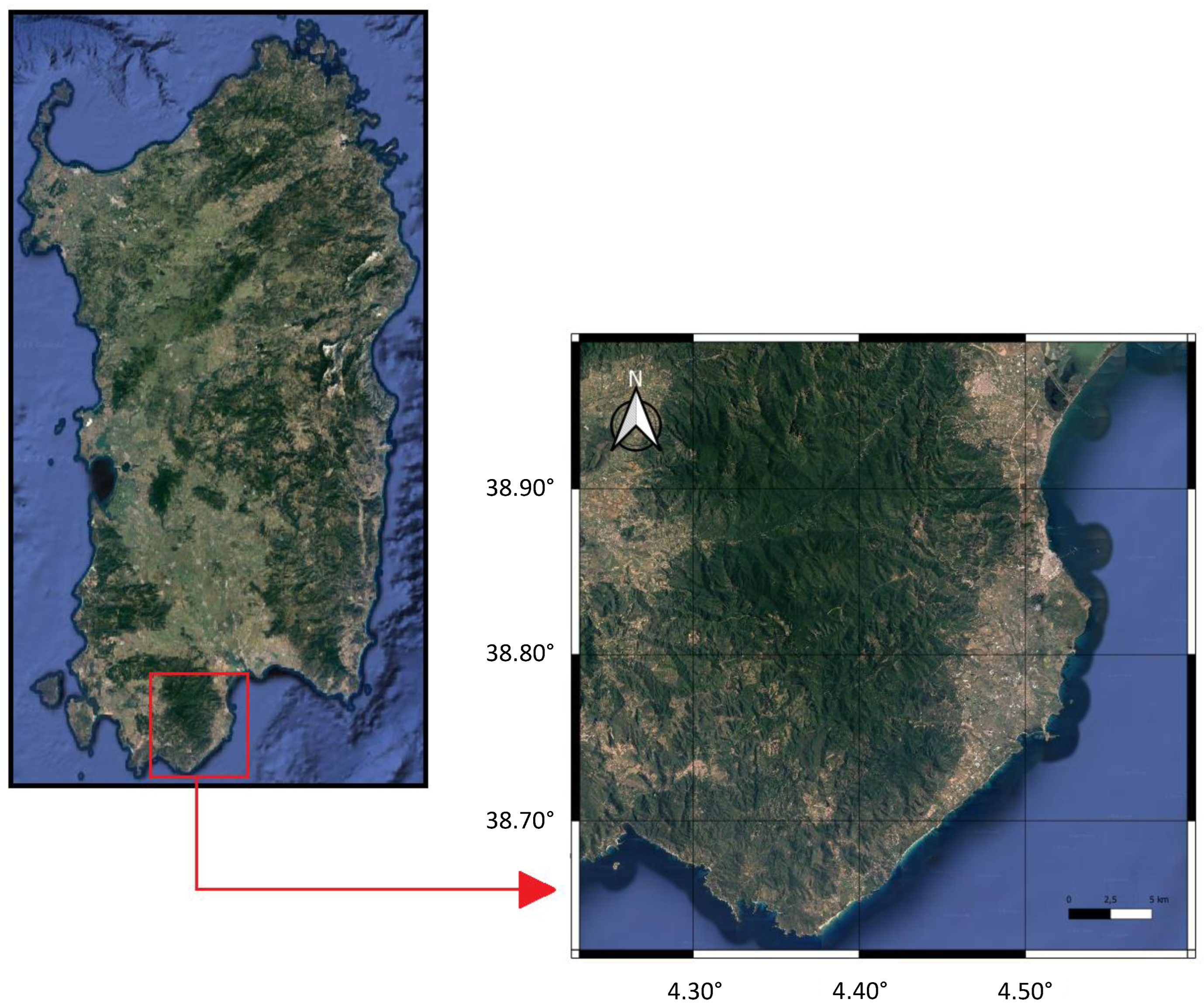
Figure 3.
Combination of Above Ground Biomass and Dryness Map into 6 classes. Where the terms: "Low", "Med" and "High" stand for Low, Medium and High Density
Figure 3.
Combination of Above Ground Biomass and Dryness Map into 6 classes. Where the terms: "Low", "Med" and "High" stand for Low, Medium and High Density
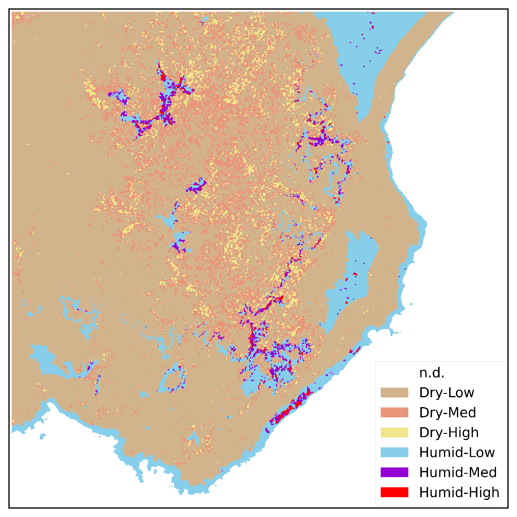
Figure 4.
Scheme of proposed CNN.
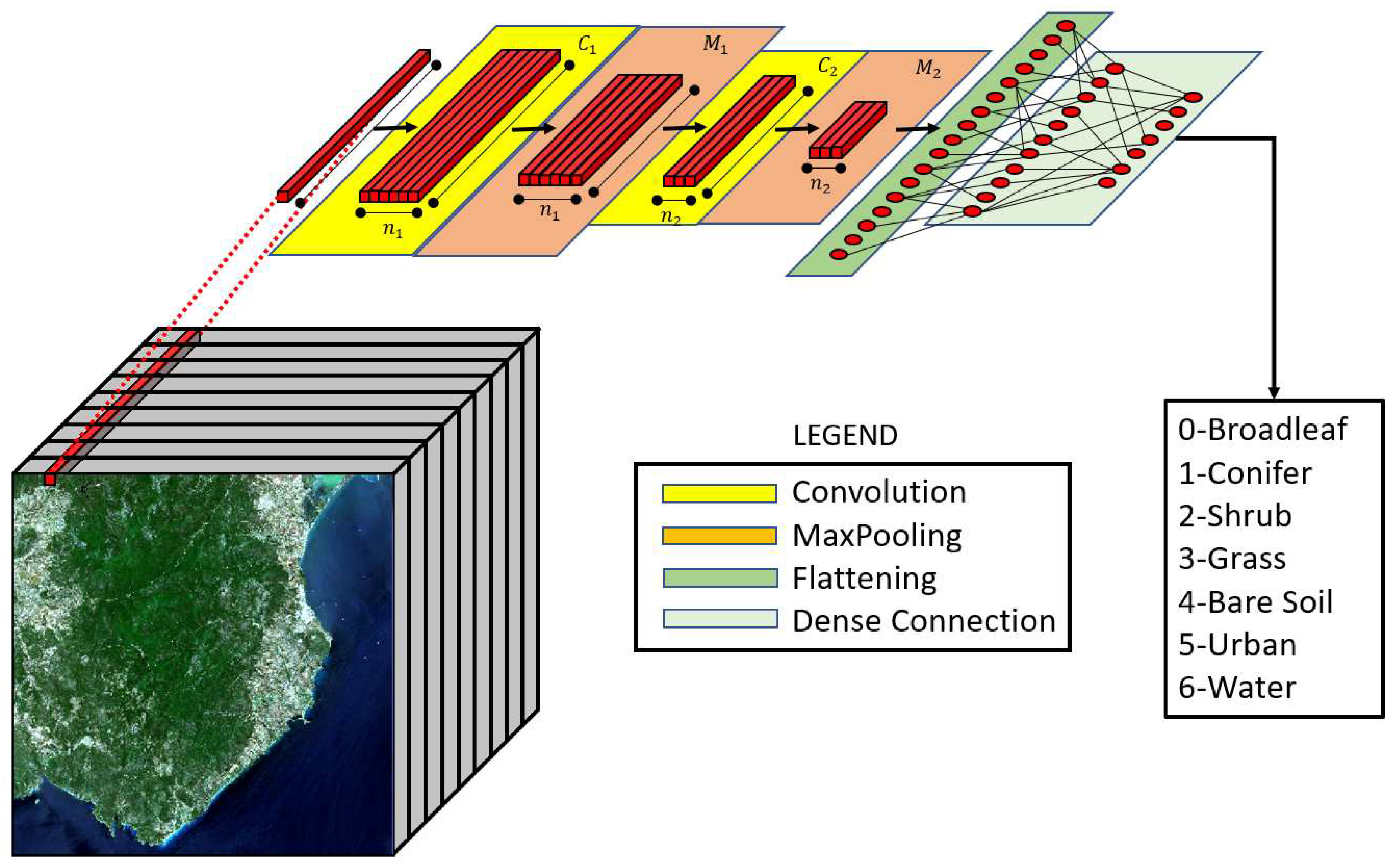
Figure 5.
Segmentation and Confusion Matrix Results
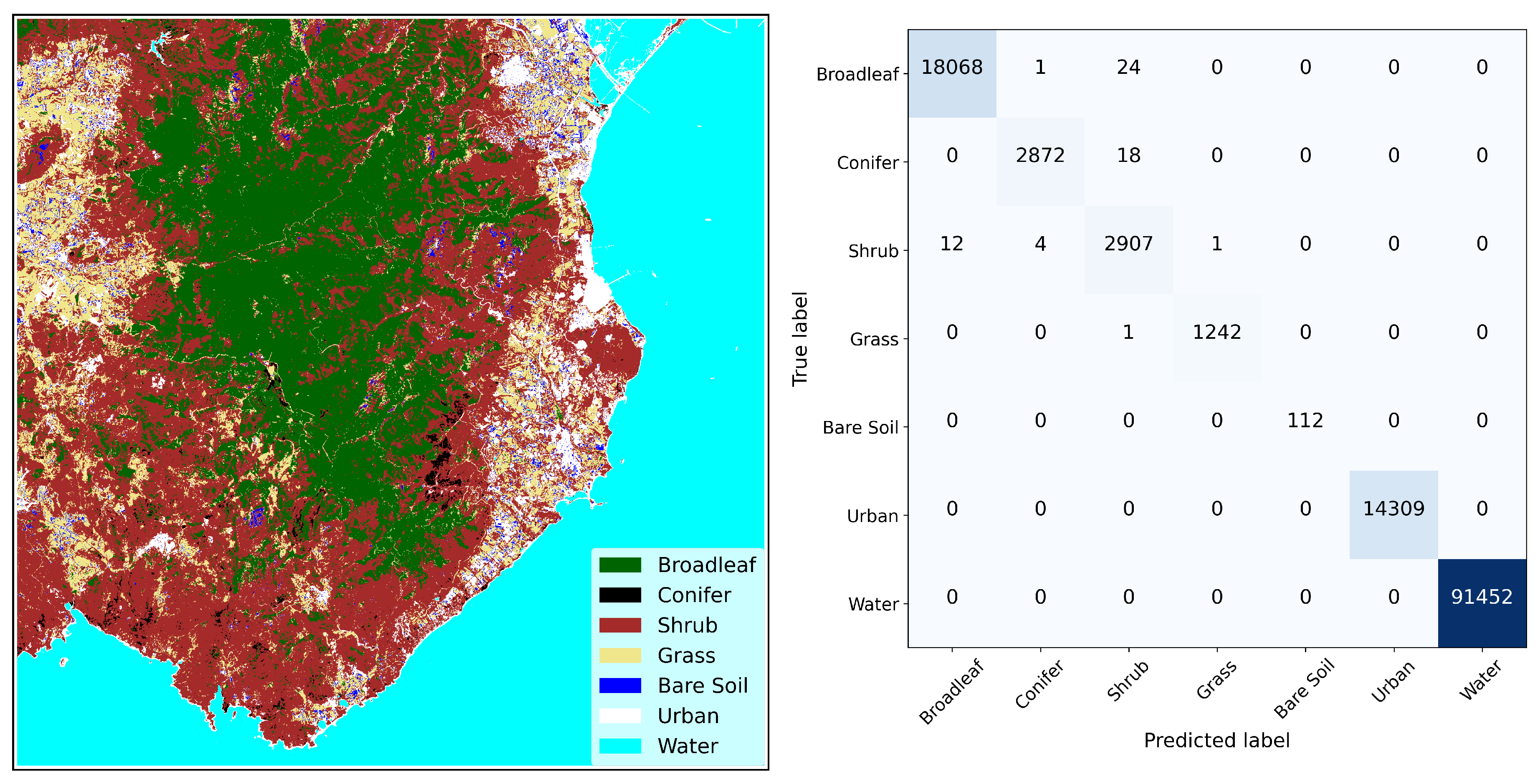
Figure 6.
Fuel Map Adaptation to Scott/Burgan.
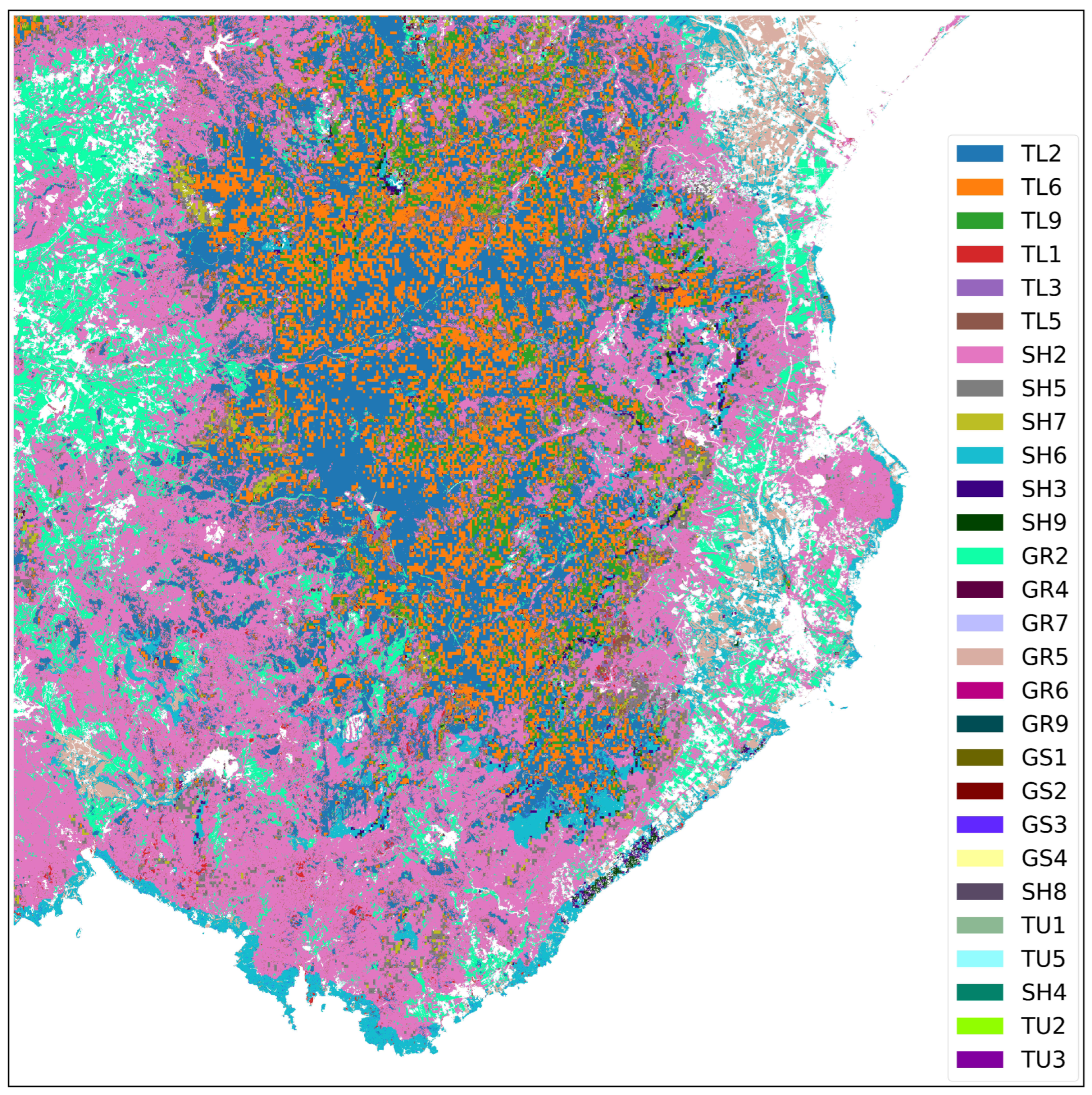

Table 1.
Index referred to Sentinel-2
| Index | Description |
|---|---|
| Range between -1 (non-vegetated surfaces like bare soil or water) and +1 (high density of healthy vegetation) | |
| Range between -1 (non-vegetated surfaces or stressed vegetation) and +1 (high density and healthier vegetation) | |
| Range between -1 (non-water surfaces) and +1 (high likelihood of water presence) |
Table 2.
Number of labelled reference pixels for CNN dataset
| Broadleaf | Conifer | Shrub | Grass | Bare Soil | Urban | Water |
|---|---|---|---|---|---|---|
| 18093 | 2890 | 2924 | 1242 | 112 | 14309 | 91452 |
Table 3.
Scott/Burgan Fuel Model Scheme
| Index | Description | Index | Description |
|---|---|---|---|
| GR1 | Short, Sparse, Dry Climate Grass | SH8 | High Load, Humid Climate Shrub |
| GR2 | Low Load, Dry Climate Grass | SH9 | Very High Load, Humid Climate Shrub |
| GR3 | Low Load, Very Coarse, Humid Climate Grass | TU1 | Low Load Dry Climate Timber-Grass-Shrub |
| GR4 | Moderate Load, Dry Climate Grass | TU2 | Moderate Load, Humid Climate Timber-Shrub |
| GR5 | Low Load, Humid Climate Grass | TU3 | Moderate Load, Humid Climate Timber-Grass-Shrub |
| GR6 | Moderate Load, Humid Climate Grass | TU4 | Dwarf Conifer With Understory |
| GR7 | High Load, Dry Climate Grass | TU5 | Very High Load, Dry Climate Timber-Shrub |
| GR8 | High Load, Very Coarse, Humid Climate Grass | TL1 | Low Load Compact Conifer Litter |
| GR9 | Very High Load, Humid Climate Grass | TL2 | Low Load Broadleaf Litter |
| GS1 | Low Load, Dry Climate Grass-Shrub | TL3 | Moderate Load Conifer Litter |
| GS2 | Moderate Load, Dry Climate Grass-Shrub | TL4 | Small downed logs |
| GS3 | Moderate Load, Humid Climate Grass-Shrub | TL5 | High Load Conifer Litter |
| GS4 | High Load, Humid Climate Grass-Shrub | TL6 | Moderate Load Broadleaf Litter |
| SH1 | Low Load Dry Climate Shrub | TL7 | Large Downed Logs |
| SH2 | Moderate Load Dry Climate Shrub | TL8 | Long-Needle Litter |
| SH3 | Moderate Load, Humid Climate Shrub | TL9 | Very High Load Broadleaf Litter |
| SH4 | Low Load, Humid Climate Timber-Shrub | SB1 | Low Load Activity Fuel |
| SH5 | High Load, Dry Climate Shrub | SB2 | Moderate Load Activity Fuel or Low Load Blowdown |
| SH6 | Low Load, Humid Climate Shrub | SB3 | High Load Activity Fuel or Moderate Load Blowdown |
| SH7 | Very High Load, Dry Climate Shrub | SB4 | High Load Blowdown |
Table 4.
Adaptation of the fuel types to the Scott/Burgan system, with the symbols BL, CF, SH, GR, GS, TS, and TSG representing Broadleaf, Conifer, Shrub, Grass, Grass-Shrub, Timber-Shrub, and Timber-Shrub-Grass class, respectively.
Table 4.
Adaptation of the fuel types to the Scott/Burgan system, with the symbols BL, CF, SH, GR, GS, TS, and TSG representing Broadleaf, Conifer, Shrub, Grass, Grass-Shrub, Timber-Shrub, and Timber-Shrub-Grass class, respectively.
| Dry-Low | Dry-Med | Dry-High | Hum-Low | Hum-Med | Hum-High | |
|---|---|---|---|---|---|---|
| BL | TL2 | TL6 | TL9 | TL2 | TL6 | TL9 |
| CF | TL1 | TL3 | TL5 | TL1 | TL3 | TL5 |
| SH | SH2 | SH5 | SH7 | SH6 | SH3 | SH9 |
| GR | GR2 | GR4 | GR7 | GR5 | GR6 | GR9 |
| GS | GS1 | GS2 | SH7 | GS3 | GS4 | SH8 |
| TS | TU1 | TU1 | TU5 | SH4 | TU2 | TU2 |
| TSG | TU1 | TU1 | TU5 | SH4 | TU3 | TU3 |
Table 5.
Comparison in terms of Accuracy, Recall, and F1 scores.
| Accuracy | Recall | F1-Score | |
|---|---|---|---|
| CNN | 0.99% | 0.99% | 0.99% |
| RF | 0.99% | 0.99% | 0.98% |
| SVM | 0.99% | 0.98% | 0.98% |
Table 6.
Comparison in terms of Validation Accuracy for Broadleaf, Conifer, Shrub and Grass classes
| Broadleaf | Conifer | Shrub | Grass | |
|---|---|---|---|---|
| CNN | 0.99% | 0.79% | 0.76% | 0.84% |
| RF | 0.99% | 0.70% | 0.77% | 0.81% |
Disclaimer/Publisher’s Note: The statements, opinions and data contained in all publications are solely those of the individual author(s) and contributor(s) and not of MDPI and/or the editor(s). MDPI and/or the editor(s) disclaim responsibility for any injury to people or property resulting from any ideas, methods, instructions or products referred to in the content. |
© 2023 by the authors. Licensee MDPI, Basel, Switzerland. This article is an open access article distributed under the terms and conditions of the Creative Commons Attribution (CC BY) license (http://creativecommons.org/licenses/by/4.0/).
Copyright: This open access article is published under a Creative Commons CC BY 4.0 license, which permit the free download, distribution, and reuse, provided that the author and preprint are cited in any reuse.


