
Submitted:
07 January 2025
Posted:
08 January 2025
You are already at the latest version
Abstract
High-resolution Sentinel-2 imagery combined with a deep learning (DL) segmentation model offers a promising approach for accurate mapping of small and fragmented agricultural burn areas. Initially, the model was trained using ICNF burn area data from Portugal to capture large fire and burn area delineation, thereby achieving moderate accuracy. Subsequent fine-tuning using annotated data from Punjab improved the model’s ability to detect small burn patches, demonstrating higher accuracy than the baseline Normalized Burn Ratio (NBR) Index method. On-ground validation using buffer zone analysis and crop field images confirmed the effectiveness of DL approach. Challenges such as cloud interference, temporal gaps in satellite data, and limited reference data for training persist, but this study underscores the methodogical advancements and potential of DL models applied for small burn area detection in agricultural settings. The model achieved overall accuracy of 98.7%, a macro-F1 score of 97.6%, IoU 0.54, and a Dice coefficient of 0.64, demonstrating its for detailed burn area delineation capability. The model can capture burn area smaller than 250m2, but the model at present is less efficient at representing the full extent of the fires. Overall, outcomes demonstrate the model’s applicability to generalize to a new domain despite regional differences among research areas.
Keywords:
burn areas
; crop residue burning
; deep learning
; neural networks
; transfer learning
1. Introduction
Crop residue burning or prescribed burning or agricultural burning is widely used agricultural practice for biomass removal, particularly in regions such as India, where its combustion provides a quick and cost-effective solution for post-harvest residue management [1,2]. Following the success of the Green Revolution, most farmers in India have shifted to a double crop system (also known as the rice–wheat system), consequently increasing food production but also necessitating earlier rice harvests to accommodate wheat sowing. Mechanized harvesters, which leave behind smaller residue fragments, have made residue disposal even more challenging. Therefore, farmers embrace open burning of residue as an easy and inexpensive and easy alternative [3,4,5].
Widespread practice of residue burning has become a significant environmental hazard. This open burning is a prominent source of particulate matter and gaseous pollutants (PM 2.5, black carbon) [6], degrading air quality and causing deleterious effects on climate and human health [7,8]. These emissions have also been linked to Arctic warming caused by BC deposition from agriculture and forest fires [9]. Despite known adverse effects, there is a considerable information gap on emissions produced by burning crop residues, especially small fires, and their growing effects on air quality health [3,10].
A main challenge hindering the understanding of burning’s contribution to emissions is the lack of accurate burn area assessment [11], which are crucial for climate models and fire emission inventories[12,13]. Current emission inventories such as GFED, FINN, and EDGAR present large degrees of uncertainty, primarily because of undetected small fires[14,15,16]. The applications of burn area assessments extend beyond scientific research and are vital for land management, environmental protection agencies, and public health organizations. These data provide insights into the immediate and long-term effects of fires on ecosystems and also guide recovery and reforestation strategies [17,18]. Furthermore, accurate burn area assessment is important to support international initiatives such as the Kyoto Protocol and the Paris Agreement (COP21) to manage fire emissions and to help monitor progress toward the achievement of Sustainable Development Goals (SDGs) as outlined by the United Nations [19].
Several factors contribute to burn area estimation inaccuracy, partly because of the dependence on coarse-resolution satellites such as MODIS and VIIRS for global and regional burn area products [20]. Widely used global burn area products MCD64A1 and FIRECC151, which respectively have resolutions of 500 m and 250 m, are based on thermal anomalies and reflectance data, making it difficult to detect small agriculture fires [11,18]. For instance, a recent study in Africa using Sentinel-2 observations revealed 1.8 times more burn area than that detected by MODIS [21], underscoring the limitations of well-established data based on MODIS. Unlike forest fires or wildfires, agricultural burning often occurs in small patches and sometimes without active flames. Unlike forest fires or wildfires, agricultural burning often occurs in small patches and sometimes without active flames. These characteristics cause the small burn areas to be overlooked, emphasizing the need for high-resolution satellite data and better approaches to enhance burn area estimation accuracy [18,22].
2. Related Work
Current mapping algorithms such as Moderate Resolution Imaging Spectroradiometry (MODIS) derived global burn area products MCD45A1 [23] and MCD64A1 [24] are effective for large and active fires but they have difficulty capturing small fires, especially those in agricultural areas. Major challenges are posed by heterogeneous landscapes, fire durations, patterns, and anthropogenic changes (plowing and seeding) [11]. Although MODIS offers good coverage, its coarse resolution (500 m) often misses fires smaller than 100 hectares. In addition, the regional burn area product MCD14ML [25], which can capture the full extent of the burn area of croplands, has been found to underestimate the total burn area [26], leading to a potential underestimation of up to ten times in agricultural regions [4]. Similarly, burn area products based on the Visible Infrared Imaging Radiometer Suite (VIIRS) at the moderate resolution of 250 m also present mixed pixel issues, whereby a pixel includes both burned and unburned regions, with false detection over water bodies [27,28]. Such inaccuracies in detection underscore the need for additional research and development of complementary methods and the use of higher resolution sensors to improve estimation of the burn area.
In recent years, the use of neural networks has shown enormous success in remote sensing applications. Early studies such as [29], used a supervised Adaptive Resonance Theory (ART) neural network to detect forest fires in Spain using NOAA-AVHRR imagery to classify the burn area image pixel-by-pixel. Later, several other studies were reported, using similar neural networks for burn area mapping. For instance, Brivio [30] used multilayer perceptron (MLP) networks with SPOT-VEGETATION data to map burn areas in sub-Saharan Africa. This neural network model exploited the spectral signals of burned areas and provided spatial and temporal information related to the burned areas. Other neural networks that have shown promising success in remote sensing applications are convolutional neural networks (CNNs) consisting of neurons that are not fully connected but which are rather only connected to those with receptive neighborhoods. With their ability to represent nonlinear functions and generalize the learned features, they are also designated as deep learning (DL) model architectures [38] and are used frequently. They show enormous potential for several image segmentation tasks involving clouds [31], water [32], urban ares [33] and vegetation types [34].
Despite its immense potential, burn area segmentation using deep neural networks is challenging because of the scarcity of training data. Recent studies using DL for burn area mapping include a developed BA-Net model based on CNN with Long Short Term Memory (LSTM) [43] and VIIRS reflectance data used to map wildfires and forest fires [35]. [36] utilized a U-Net architecture DL model to develop a fully automatic processing chain to segment vegetation fires. The trained model with Sentinel-2 imagery as an input showed better results against the Random Forest classification. Another recent work by [37], trained a U-Net-based DL model over Portugal and tested the Transfer learning applicability of the model to analyze local burn area dynamics in West Nile, northern Uganda. The model exhibited the promising application of U-Net and the transferability of learned features in capturing small burn areas, along with related details of large burn areas over a new domain. These studies have been important sources of information and motivation for this experiment conducted in Punjab, India.
Data scarcity for economically developing regions presents a unique challenge for DL applications for burn area assessment and fire monitoring. Our study area Punjab lacks reliable ground truth data for training the model. Therefore, we propose a transfer learning approach to estimate small agricultural burn areas in Punjab. By training a model on a source domain (Portugal) using The Institute for Nature Conservation and Forests (ICNF) dataset, we can apply and fine-tune it for Punjab, overcoming data limitations with hand-annotated data. This study was conducted to 1) train the model on the source domain, 2) apply transfer learning and fine-tuning to the target domain for improved prediction, and 3) assess changes and trends of small agricultural burn areas throughout the post-harvest season in Punjab.
3. Data and Method
3.1. Study Area
Figure 1.
Land Use Land Cover map over Punjab, 2018. The yellow region represents the area under intense agricultural cultivation. Image credit: National Natural Resource Management, ISRO [38].
Figure 1.
Land Use Land Cover map over Punjab, 2018. The yellow region represents the area under intense agricultural cultivation. Image credit: National Natural Resource Management, ISRO [38].
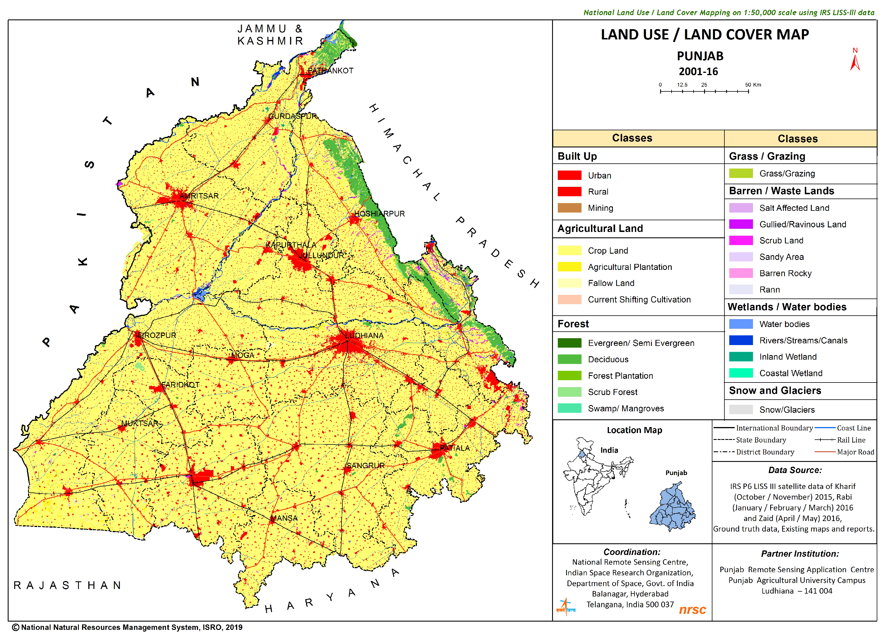
Punjab state (Figure 1), located in the northern part of India, has a geographical area of 50,362 , of which 40,230 is under cultivation (Dept. of Agriculture and Farmers Welfare, Govt. of Punjab). Punjab is known as the "breadbasket" of India, producing two-thirds of the nation’s food requirements. After the monsoons, approximately 7 million tons of crop residues are burned annually in Punjab. [39].
Agricultural burning is common in many parts of India, but the situation in Punjab is unique and severe because of several factors: 1) Double cropping systems originating with the Green Revolution have led to wheat–rice double cropping systems in India. This intensive agricultural practice produces vast quantities of crop residue that must be cleared quickly because of the narrow time window between crop harvesting and sowing [40], 2) A shift toward mechanized harvesters has left behind large amounts of scattered, root bound residue across the fields, prompting farmers to use open burning as a quick and inexpensive solution to clear their fields [3,4]. 3) Meteorological conditions such as weak winds and changing weather patterns also exacerbate air quality. The entire Indo-Gangetic plain, which supports a large population, experiences heavy smog during October–November because light winds trap pollutants and weak north-westerly winds push them toward densely populated urban areas such as New Delhi, exacerbating air pollution and health concerns [41,42]. Every year the entire region is enveloped in smoke and haze as a result of intense residue burning, which produces pollutants such as , CO, , NO, and NMHCs. These emissions not only disrupt regional atmospheric chemistry: they pose important public health hazards for nearby densely populated areas [43,44].
Figure 2.
Workflow.
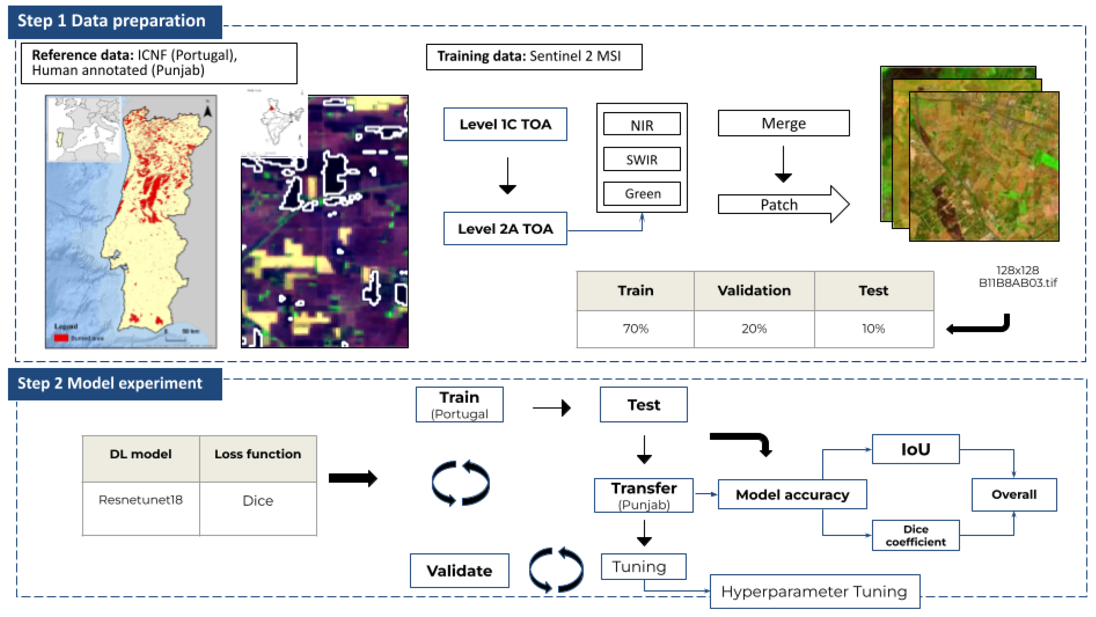
As the training dataset for our study, we used Sentinel-2 Multispectral Instrument (MSI) Level 1C data, which provide Top of Atmosphere (TOA) reflectance at 20 m resolution. We use reference data of two types. For initial training in Portugal, we used the ICNF dataset for 2016 and 2017 to train our model during the fire season. The deep learning model we used is based on the Resneunet18 architecture: a robust framework known for its effectiveness in image segmentation tasks, especially when distinguishing between burned and unburned areas [45]. Initially, we trained our model using the ICNF dataset to capture the general features of burned areas. Later, we fine-tuned the model using hand-annotated data to enhance the model’s performance and to adapt it to local conditions of Punjab.
The hand-annotated data were created for a 200 km2 area in Punjab: roughly equivalent to two Sentinel-2 tiles. The fine-tuning step involved adjusting hyperparameters of the model based on the Punjab data and re-evaluation of their accuracy to ensure optimal performance in detecting burn areas under different geographical and environmental conditions. The model’s accuracy was assessed using several key metrics including IoU and the Dice score (section 3.7.1). These metrics helped us gauge the model’s capability of identifying and delineating burned areas accurately. The next section presents a detailed discussion of each step involved in the data pipeline and model experiment.
3.2. Data Acquisition and Atmospheric Correction
To analyze the burn areas over the source domain (Portugal) and the target domain (Punjab), we used the available single Sentinel-2 Level 1C Top of Atmosphere (TOA) reflectance data with less than 20% cloud cover, allowing us to capture and analyze the burn area extent from individual images throughout the burning season. The Copernicus Sentinel-2 program consists of two sun-synchronous polar-orbiting satellites, Sentinel-2A and Sentinel-2B, which have a swath width of 290 km and a revisitation period of 5 days. The Multispectral Instrument (MSI), a key payload onboard the Sentinel satellites, provides high spatial resolution imagery. MSI covers 13 spectral bands with spatial resolutions of 10–60 m. Sentinel-2 MSI data are available for two product levels: Level 1C (L1C) and Level 2A (L2A). L1C data represents TOA reflectance and L2A provides atmospherically corrected bottom-of-atmosphere (terrain-corrected and cirrus-corrected reflectance images) according to the sen2cor algorithm [46]. Global availability of L1C data starts from 2015, whereas L2A data are available from 2017.

Table 1.
Sentinel-2 spectral band characteristics adapted from an earlier report [47].
Table 1.
Sentinel-2 spectral band characteristics adapted from an earlier report [47].
| Band | Description | Bandwidth (nm) | Central wavelength (nm) | Spatial resolution (m) |
|---|---|---|---|---|
| 1 | Aerosol | 20 | 443 | 60 |
| 2 | Blue | 65 | 490 | 10 |
| 3 | Green | 35 | 560 | 10 |
| 4 | Red | 30 | 665 | 10 |
| 5 | Vegetation edge | 15 | 705 | 20 |
| 6 | Vegetation edge | 15 | 740 | 20 |
| 7 | Vegetation edge | 20 | 783 | 20 |
| 8a | NIR | 115 | 842 | 10 |
| 8b | Narrow NIR | 20 | 865 | 20 |
| 9 | Water vapor | 20 | 945 | 60 |
| 10 | Circus | 30 | 1380 | 60 |
| 11 | SWIR1 | 90 | 1610 | 20 |
| 12 | SWIR2 | 180 | 2190 | 20 |
To conserve computation resources for our analysis, we opted to use L2A products whenever available. Alternatively, we acquired L1C data and converted it into L2A using the sen2cor algorithm [46]. In the case of Portugal, we aimed at reproducing similar model accuracy to that of an earlier study [37]. Portugal experiences numerous fire events in August. Especially in 2017, a record-breaking number of fire events occurred, accounting for approximately 500,000 ha of total burned area [48,49]. This dataset with unusually numerous burned areas can be useful to ensure that models can learn burn area features rigorously. In Portugal, we specifically examined periods of peak fire activity during 2016–2017 to ensure a maximum burn area. Specifically, we targeted August for Portugal (2016 and 2017). In Punjab, we particularly examined the post-monsoon burning season of October–November for Punjab (2020–2023). The data were downloaded using the Python API from the Copernicus Data Space. The API used to download the data is available in an earlier report [50].
3.3. Preparation of Reference Data
ICNF provides a regional database in vector files. The ICNF burn area dataset is based on a cartographic method by which burn area polygons are created using a semi-automatic classification process using Sentinel, LANDSAT, and MODIS satellite images. Additional details are available in the literature [51]. The hand-labelled dataset has high quality, giving a good idea of burn extents. Moreover, the dataset is publicly accessible. For our analyses, the ICNF data were acquired for August 2016 and August 2017. An important domain difference exists between Punjab and Portugal in terms of climate, topography, and fire event types. To compensate for that gap, hand annotation of burn areas over 200 (equivalent to two sentinel tiles) was performed. Our objective was to encompass various burn areas. For that reason, we selected regions with a high density of MODIS and VIIRS fire hotspots. MODIS fire hotspot data give a good approximate idea about where most fire events are occurring. Therefore researchers have often relied on fire hotspot information to assess burn areas [52,53].
To ensure good quality and better acclimatization of the model, we considered several factors for hand-annotation of the data: a) use of RGB Sentinel images for visualization and manual checking of the presence and absence of burn scars, b) human capability based on past experience and observation to distinguish burned and unburned areas, c) presence of active flame and smoke, and d) cross-verification of hand annotations with the closest available Google Earth (Alphabet Inc.) images. To consider annotation over agricultural land explicitly, we used land use land cover data to exclude all other land types, especially for urban areas and aquatic bodies. The annotation was performed in two sets (Figure 4): Annotation 1 (Ano1) and Annotation 2 (Ano2), over two adjacent areas covering 100 km2 each. Actually, Ano 1 had more common features such as large uninterrupted patches of agricultural land, absence of big water bodies, and more numerous observable burned agricultural fields. By contrast, Ano 2 included more diverse features such as river streams and big urban areas and more numerous observable non-burned agricultural fields. The two sets of annotations were performed on closely proximate dates and during peak fire seasons. The motive behind this step is to study the model’s learning and transferable capacity of learned features while fine-tuning using annotation data of different types. The ultimate goal was to enhance model robustness not only by making accurate predictions over burned areas, but also to make minimum false predictions over non-burned or non-agricultural areas.
Figure 3.
Location and area for hand annotated data over Punjab.
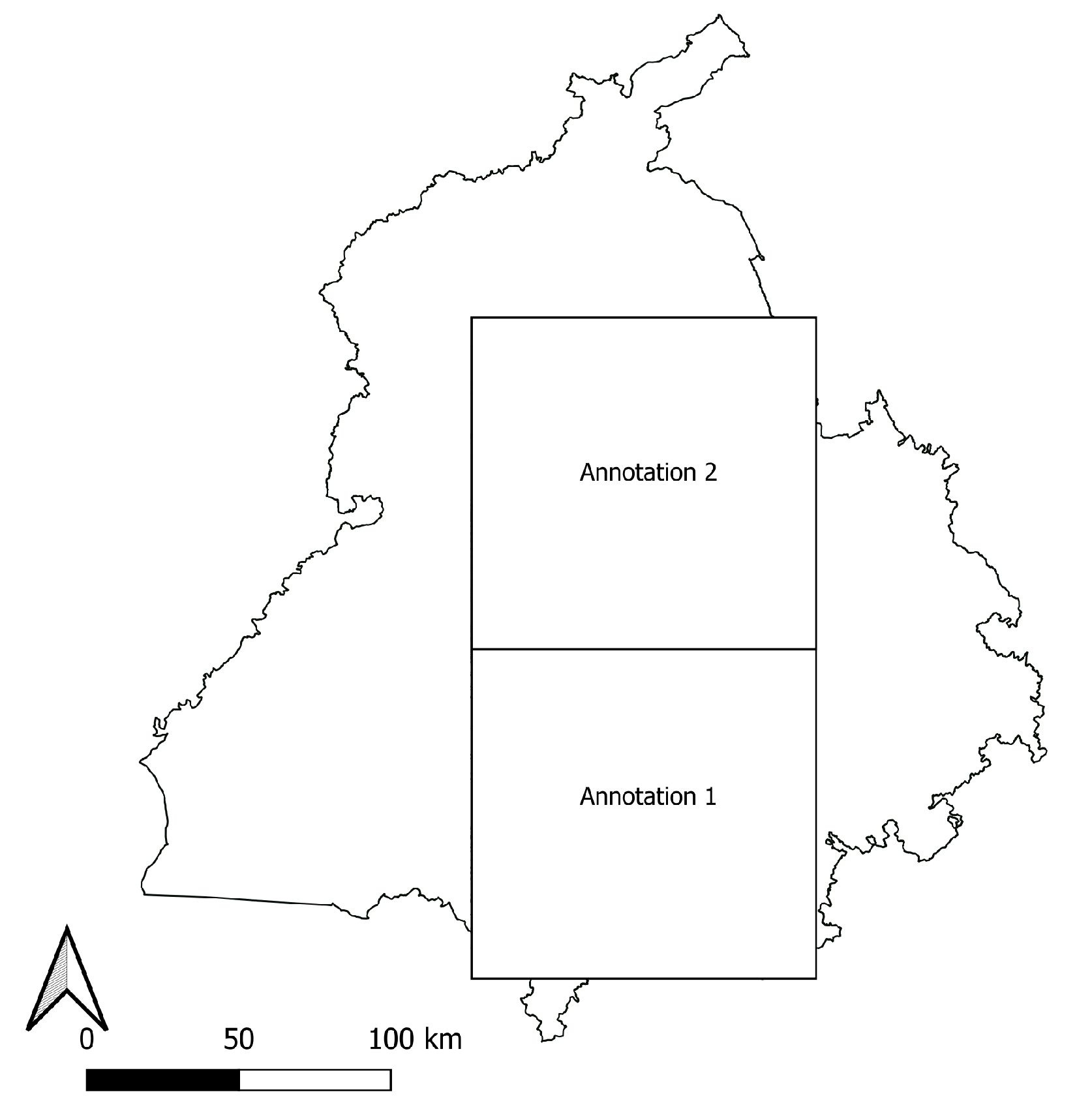
Figure 4.
Example of Ano 1 data (left) showing the presence of agricultural burn areas (common features) and Ano 2 data (right) showing the presence of diverse features such as rivers, unburned areas, and non-agriculture areas.
Figure 4.
Example of Ano 1 data (left) showing the presence of agricultural burn areas (common features) and Ano 2 data (right) showing the presence of diverse features such as rivers, unburned areas, and non-agriculture areas.
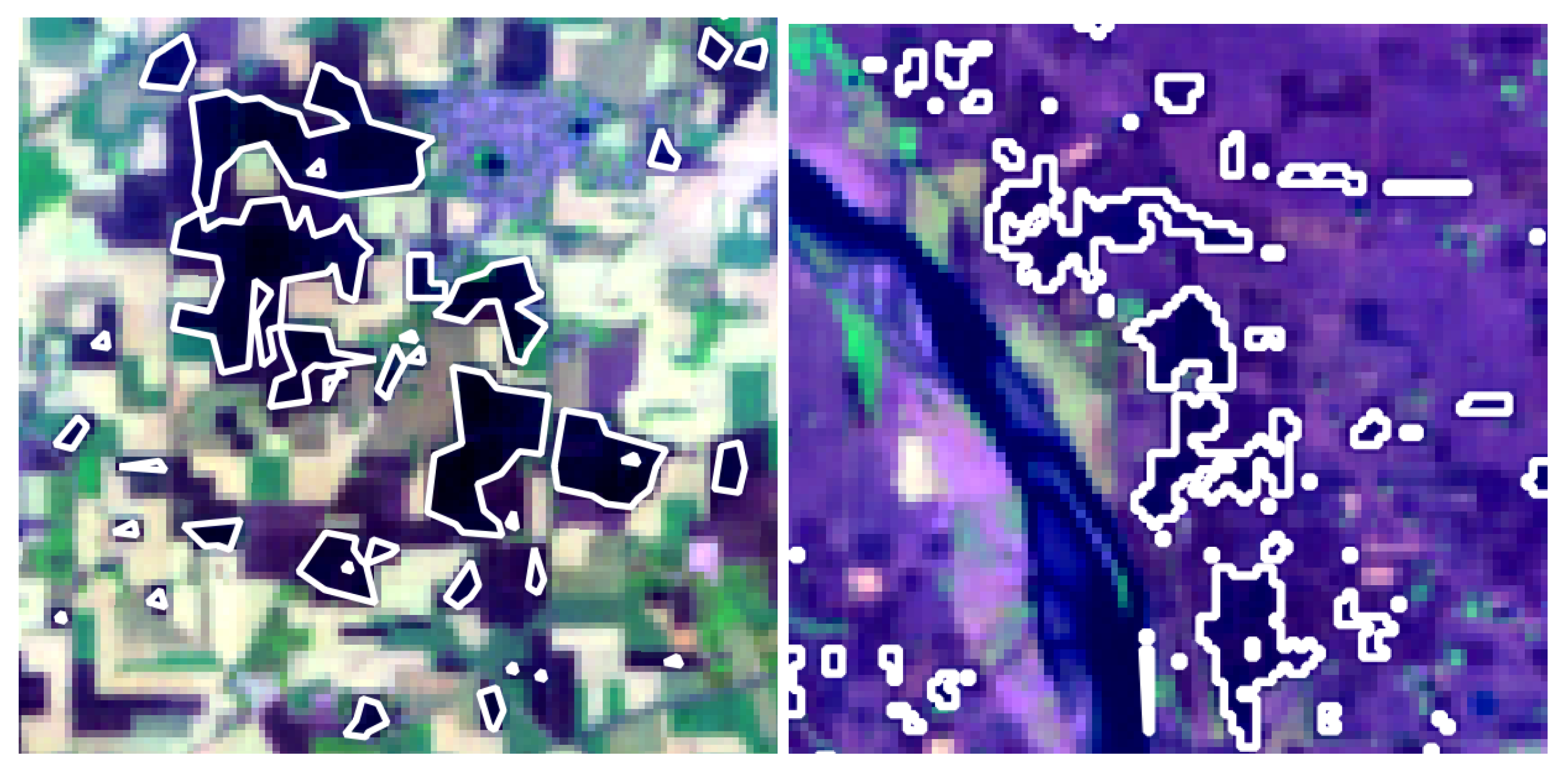
Figure 5.
Cross-verification of annotated burn areas using the closest available Google Earth (Alphabet Inc.) images.
Figure 5.
Cross-verification of annotated burn areas using the closest available Google Earth (Alphabet Inc.) images.
3.4. Data Pipeline
The data pipeline is divided into four stages, as adapted from an earlier study [37]).
For these analyses, we are interested in exploiting the spectral properties of the following three bands: near-infrared (8a), green (3), and shortwave–infrared (11). The bands are selected because of their spectral sensitivity toward change in unburned and burned vegetation. Selected bands were stacked together to create false-color images for both Portugal and Punjab. Merged false-color images were extracted into patches of 128 × 128 pixels. The patch size of 128 × 128 was selected as a good optimal middle ground between detailed retention of spatial context and the need for intensive computational resources.
Extracted patches were stacked along with the corresponding reference dataset. Incomplete or broken patches were discarded. Details of the four stages are discussed hereinafter. Merge bands (Stage 1): Combine the atmospherically corrected Green, NIR, and SWIR bands of Sentinel-2 data to create false-color images that emphasize burned areas. Normalize the values to the 0–255 color scale. Extract patches (Stage 2): Match ground truth data to false-color images based on area and date. Extract small 128 × 128 patches from both datasets to reduce memory usage during training. For Portugal, we set a time frame of 30 days to consider a maximum observation by Sentinel-2. Filter patches (Stage 3): Remove empty or damaged patches from the datasets to ensure data quality. Split patches (Stage 4): Randomly split training patches into a 70% training dataset and a 20% validation dataset and 10% test dataset.
3.5. Baseline Model
To put the model performance into context, a baseline model was tested using the same validation dataset as that used for the DL model. The baseline model is based on calculation using the NBR index method [54]. The NBR is a popular index to calculate burn area and burn severity along with its derivatives dNBR and rNBR [55]. NBR is based on the spectral response difference between near infrared (NIR) and shortwave infrared (SWIR). For this experiment, we applied NBR as baseline model to the same validation dataset used for the DL model. The NBR value for each pixel was calculated using the following formula:
Therein, the NBR values range from -1 to +1. Higher NBR values denote healthy vegetation, whereas lower values suggest recently burned vegetation or bare ground. To generate the baseline prediction, we initialized an array and iterated over each validation image. For pixels meeting the burn threshold (NBR < 0.3) [ 58 ], the baseline prediction array was updated to classify the pixel as burned. The baseline predictions for the entire dataset were then evaluated using the same evaluation metrics.
3.6. Model Framework
Segmentation, as the name implies, involves dividing features within an image into distinct classes: in this case, burned or burned. Semantic segmentation assigns each pixel of an image to a specific class. For this task, we implemented a deep learning segmentation model based on U-Net architecture within the PyTorch lightning framework. Originally developed for biomedical image segmentation [45], this type of network is easily trainable and suitable for small datasets [59]. U-Net is based on CNNs, where the layers are not fully connected. Therefore, the decisions are made locally. U-Net receives raw images as input and produces a segmented image as an output. The network architecture comprises an encoder and decoder, giving it a distinct U shape. The encoder or the contracting path captures context and complex features through convolution and pooling layers while the decoder part facilitates feature localization by combining upsampled outputs with corresponding encoder features through concatenations. Finally, the vector is restructured into a 2D image using transposed convolutions [45].
3.6.1. Hyperparameter Setting
The model’s training is conducted using specific hyperparameters and strategies chosen based on recommendations and best practices from developer communities and scientific reports. As discussed earlier, the segmentation model used for this experiment has an encoder–decoder part, an encoder based on Resnet [56] and a decoder based PSPnet [57], a popular choice for image-related tasks because of its balance between performance and computational efficiency. Batch size: training in the source domain begins with a batch size of 32 to enhance model generalization and to reduce overfitting [58]. For transfer learning in the target domain, we reduced the batch size to 16, a common strategy to deal with smaller and domain-specific datasets. A smaller batch size provides finer gradient updates, helping the model to adapt more precisely to the nuance of the new domain [58]. Weight Initialization: Rectified Linear Unit (ReLu) is applied as an activation function for the convolutional layers in the network [56] Optimizer: For network optimization, Adam optimizer is used, known for its efficiency in handling sparse gradients and adaptive learning rate capabilities [59]. The learning rate is set to 0.0003. In the fine-tuning process, the learning rate is reduced to 10 times. Regularization: A Weight decay of 0.0001 is applied to regularize the model and reduce overfitting. The training is set to 50 epochs for the source domain and up to a maximum of 45 for the target domain. Early stopping is implemented to halt training if validation loss does not improve over 30 consecutive epochs. Additionally, a step scheduler adjusts the learning rate based on changes of the validation loss, enhancing the convergence and avoiding overfitting. Loss Function: because this study presents a binary class segmentation problem, Binary Cross Entropy (BCE) was implemented as the most suitable loss function [64]. [60].
The model framework is implemented using PyTorch with PyTorch lightning as the high-level interface for training. Computations were conducted using Fujitsu Prime HPC FX1000 and Fujitsu Primergy GX2570 (Wisteria/BDEC-01). Details were presented in an earlier report [61]. This powerful computing environment, equipped with (A100-SXM4-40GBs; NVIDIA Corp.) provided the necessary computational resources to accommodate the intensive demands of deep learning.
3.7. Experiment Setup
The DL experiment was conducted in two main phases: 1) model initial training over the source domain (Portugal) and 2) transfer learning and fine-tuning over the target domain (Punjab). During the first phase, the model was trained for two consecutive fire seasons in Portugal: 2016 and 2017. The model associated with the lowest training loss was saved. The training was limited carefully to prevent overfitting and ensure generalizability to prevent the model from becoming overly specialized in terms of source domain-specific features. Overfitting can engender poor performance when applied to new regions with different patterns, such as Punjab. Some studies such as [56,62] have demonstrated that excessive training with one region often reduces model transferability. The second phase involves fine-tuning the pre-trained model for Portugal using annotated data from Punjab. We used transfer learning, allowing the model to adapt its learned features to different geographical features for the Punjab region under varying hyperparameters and weight update conditions. Additionally, we experimented with network architecture modification by freezing (keeping the weight of certain layers constant) and unfreezing (allowing the weights to be updated during training) the encoder layers and the use of two sets of annotation data with diverse features to examine the feature transferability of the model at different stages. Further details of each conducted experiment can be found in Appendix B.
3.7.1. Evaluation Metrics
To evaluate the model performance on the segmentation task, we used key evaluation metrics: the Dice score and Intersection over Union (IoU). Intersection over Union (IoU), also known as the Jaccard Index, is the ratio of the intersection to the union of the ground truth data and the model’s predictions. It is a commonly used metric for evaluating segmentation tasks
Intersection over Union (IoU): also known as the Jaccard Index is the ratio of the intersection to the union of the ground truth data and the model’s predictions. It is a commonly used metric for evaluating segmentation tasks [63]. Mathematically, it is defined as
where A represents the set of ground truth pixels and where B represents the set of predicted pixels.
Dice similarity coefficient The Dice Similarity Coefficient (DSC), commonly known as the Dice Score, represents the spatial overlap between two segmentations: ground truth data and model predictions. DSC is another standard metric used to evaluate the accuracy of the image segmentation mode [64]. Mathematically, the Dice Score is defined as shown below.
Both the IoU and Dice scores assess the spatial accuracy of the semantic segmentation task [65,66]. The Dice Score can quantify the overlap between two binary sets, making it particularly useful for assessing segmentation performance [66]. A high IoU value (close to 1) shows strong alignment between predicted and actual data. The values are useful for class-imbalanced segmentation by particularly addressing the overlapping regions. Similarly, a high Dice Score (close to 1) reflects high similarity between predicted and true segmentations, indicating precise model performance. To ensure balanced evaluation and to avoid penalizing the model for correct non-detection, cases of zero overlap are assigned a perfect score of 1 because not detecting the unburn area as the burn area is also a good model performance indicator. [67]
Because the model produces segmented maps for each class, which are converted into a binary mask and to elucidate the effects of not detecting non-burned areas as burned areas, we used a confusion matrix to compare the predicted and true labels. The confusion matrix provides counts for True Positive (TP), False Positive (FP), False Negative (FN), and True Negative (TN). Using these values, we calculated the following metrics:
Precision: The ratio of true positive predictions to all positive predictions.
Recall (Sensitivity): The ratio of true positive prediction to all actual positives.
F1 score: represents the harmonic mean of Precision and Recall. It is particularly useful to assess the model performance of imbalance data.
Accuracy: is the proportion of correctly predicted instances among all predictions.
4. Result and Discussion
The training history of the DL model provides insight into the learning progression of the model in two phases. Initial training in the source domain Figure 6(a) demonstrates the loss of training and validation with Portugal data. The model starts with a higher initial loss (1.8) and converges at 0.4 after 40 epochs. This steady decrease reflects the model’s capability to generalize key features of large-scale burn areas in Portugal. Figure 6(b) presents the training history of the fine-tuned model in Punjab. Benefiting from transfer learning, the model begins with a lower initial loss (0.8) and converges quickly at 0.4 within 30 epochs. The early stabilization of both training and validation loss indicates efficient adaptation of the model to the characteristics of the burn area in Punjab. For both phases, the consistent gap separating training and validation loss indicates that the model maintains generalization without any marked overfitting.
4.1. Model Performance
To evaluate the segmentation accuracy of the burned and non-burned areas, we compared the performance of the DL model trained in Portugal, the fine-tuned model in Punjab, and the Baseline NBR model using their prediction on the test dataset. Table 2 summarizes the performance of each model under different metrics.
The performance of each model under different metrics was calculated. Findings indicate that the fine-tuned DL model outperforms the other two models across key performance metrics, including IoU, Dice, and Macro-F1 scores. The DL model trained using Portugal data achieves a Macro-F1 score of 89% and an overall accuracy of 94.5%. Although these results are satisfactory, the IoU (0.52) and Dice (0.60) show moderate overlap with the ground truth, reflecting the model’s ability to identify burned areas accurately without overfitting to the training region. The model was intentionally designed not to overly specialize in this domain to retain generalizability. The DL model fine-tuned using Punjab data shows marked improvements. The macro-F1-score increase to 97%, with overall accuracy of 98.7%. The IoU (0.54) and Dice (0.64) score reflect greater spatial overlap compared to the Portugal-trained model.
Overall, the accuracy for segmenting non-burned areas was consistently higher than that obtained for burned areas, as indicated by the higher Precision and Recall values for the non-burned areas. For the Portugal-trained model and fine-tuned model, false predictions for the burned area were primarily attributable to overestimation (false positives), although errors in the non-burned class were attributed to the missed relevant samples (false negatives). These trends are consistent with the inherent challenges of the segmentation tasks, particularly in detecting small and fragmented burn areas.
4.2. Pre-tuned vs. Fine-Tuned Model Performanc
This section presents examination of the role of fine-tuning the DL model on improved segmentation of burned area. The pre-tuned model (trained using Portugal data), as shown in Figure 7(a) struggles to generalize using data of Punjab, misclassifies urban areas as burned regions and produces poor performance with a lower IoU (0.32) and Dice (0.49) score. This poor performance demonstrates the inability of the pre-trained model to account for the regional differences and burn area characteristics of small fires, indicating a lack of sensitivity to finer details. After fine-tuning Figure 7(b) with hand-annotated data, the model improves by showing fewer false detections with a higher IoU (0.54) and Dice (0.70) score. High accuracy indicates a good shift to model adaptation over new domain and generalization of features. By contrast, baseline model Figure 7(c) based on the Normalized Burn Ratio Index method overestimates the burned regions, producing numerous false positive results over urban and healthy vegetation, resulting in low IoU (0.0) and Dice (0.0) scores. section 4.3. presents a detailed comparison with the baseline model.
4.2.1. Impact of Architectural Modification and Annotation Data on Segmentation Task
As outlined in Section 3.7 we assessed the model performance by modifying the network architecture under various conditions. The Appendix presents additional details. The modification involved the freezing and un-freezing of the encoder layers, which are common practices in transfer learning.
Freezing the layers in early stages helps to preserve general features learned from the pre-trained model, such as edges and textures which are transferable across domains [68]. By contrast, unfreezing these layers in later stages enables the model to adapt to the unique features of the target domain, refining its ability to distinguish diverse features such as bare soil, urban areas, and aquatic regions. For instance, the model with unmodified architecture in Figure 8(a) shows high false detection over bare ground and plowed areas resulting in lower IoU (0.32) and Dice (0.49) scores. The modified architecture in Figure 8(b) shows a slight but improved reduction in false positives achieving higher IoU (0.54) and Dice (0.70) scores. Although the accuracy improvement is modest, the result indicates the model’s sensitivity to diverse features.
The architectural modification also enhanced segmentation in aquatic regions. Figure 8(c) shows that the unmodified architecture struggles to distinguish aquatic regions capturing it as burn area Figure 8(c) (white circle). By contrast modified architecture Figure 8(d) reduces the error, improving the accuracy for over aquatic regions. Previous studies have shown that such staged fine-tuning enhances model sensitivity and reduces the over fitting by balancing the generalization [69,70].
Additionally, the use of two sets of annotation data (Ano 1 and Ano 2) further contributed to the enhanced segmentation in the modified architecture. The unmodified architecture Figure 8(c), and simultaneous tuning on Ano 1 and Ano2 provided a model with a wide range of features. However, this approach also diluted the capability of specialization, resulting in poor overlap and false prediction, particularly for aquatic regions and bare soil [71]. The modified architecture portrayed in Figure 8(d) used a sequential training strategy, where the pre-trained model was first tuned on Ano1 data (for details refer to Experiment L in the Appendix) and later fine-tuned further on Ano 2 data (for details refer to Experiment M in Appendix). This gradual learning process allowed the model to adapt incrementally, thereby capturing broad features initially and later refining its understanding of region-specific details.
4.2.2. Model Sensitivity over Small Burn Area
The core objective of this study is enhancement of the model’s ability to capture small burn patches. As shown in Figure 9(a) the pre-tuned model struggled with smaller fires, indicating a lack of sensitivity to finer details, leading to low segmentation accuracy. The post-tuning prediction Figure 9(a) demonstrates marked improvement in detecting small fires and burn patches, leading to higher IoU (0.72) and Dice (0.84) scores. Figure 9(c) highlights another limitation, whereby the pre-tuned model struggle to differentiate healthy vegetation from burn areas, resulting in zero overlap. In contrast Figure 9(d) shows the fine-tuned model accurately distinguishing between healthy vegetation and burn patches, and achieving higher IoU (0.73) and Dice (0.84) scores. This improved sensitivity is crucially important for generating reliable segmentation maps for agriculture fire monitoring, especially distinguishing burn areas from urban and vegetation areas.
4.3. DL Model Prediction Vs Baseline Model (Normalized Burn Ratio Index Method)
This section compares the performance of the fine-tuned DL model against the baseline model, which uses the NBR index method for detecting burn areas. The result highlights the DL model superiority in addressing the limitations inherent in the baseline model. The images show that the baseline model tends to overestimate burn areas, particularly in accurately detecting small fires and small burn areas and fragmented patches. The baseline model (NBR) demonstrates frequent overestimation of the burn area, with large false-positives over healthy vegetation. For instance,Figure 10(a), presents overestimation of burn areas, with large false-positive regions over healthy vegetation, leading to low IoU (0.04) and Dice (0.07) scores. Similarly, Figure 10(c) shows the baseline model identifying numerous small burn areas scattered throughout the image, even in regions where the ground truth indicates healthy vegetation, indicating that the model is adversely affected by spectral confusion in NIR and SWIR bands. By contrast, the fine-tuned DL model achieves more accurate prediction by leveraging its enhanced ability to learn spatial and spectral features. As seen Figure 10(b)shows that the DL model effectively captures small burn area delineations, minimizing the false positive and achieving higher IoU (0.73) and Dice (0.85) scores. This finding demonstrates the model’s capability to handle complex land cover patterns. Similarly, Figure 10(d) highlights the DL model’s accurate identification of burn areas, even in regions prone to confusion with bare ground and healthy vegetation. The DL model’s enhanced performance is reflected in improved IoU (0.35) and Dice (0.52) scores.
Both NIR and SWIR bands are sensitive to changes in vegetation and soil moisture [54]. Burned areas typically exhibit a distinct spectral signature in these bands, characterized by lower NIR reflectance and higher SWIR reflectance compared to healthy vegetation. However, bare ground and burned ground can exhibit similar spectral properties, particularly in the NIR and SWIR bands. This similarity can engender spectral confusion, where the baseline model misclassifies bare ground as burned areas. A varying degrees of vegetation cover can affect NIR and SWIR reflectance. The NBR index’s sensitivity to chlorophyll and moisture content of the ground can influence the spectral response, resembling that of burned ground and leading to false positives [72]. In contrast, the DL model leverages learned spatial and spectral patterns to distinguish between these features, providing a more robust solution for burn area detection.
4.4. Site-Validation
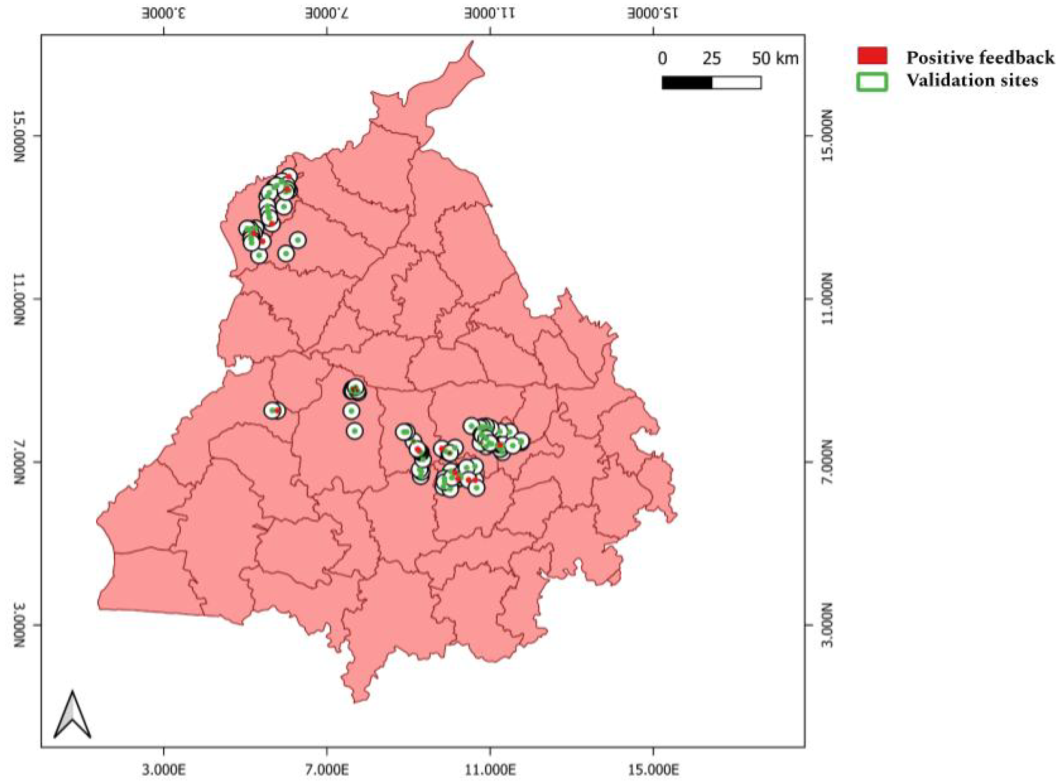
On-ground verification is necessary to elucidate the model predictions in light of actual ground truth data. To be certain that the burn area observed in the images is likely also to be detected by the model, we conducted a buffer zone analysis. To assess the model’s effectiveness over the crop-burned area, we conducted a site survey across the Punjab region. During this site survey, approximately 110 images were collected on the ground using a geolocated camera. The location and time of capture were recorded meticulously for each image. Considering the quality of images and the presence and absence of a potential burn area site, we selected 94 images suitable for site validation. All the selected 94 sites are shown in Figure 11.
We applied buffer zone analysis, a GIS technique by which a specified distance is applied around a point, line, or area to create a zone for spatial analysis [73]. This analysis was used to verify whether the burn area polygons detected by the model correspond to actual burn areas observed on the ground. We created a 500 m radius buffer zone around each location where field images were captured. The model-detected burn area data were then overlaid with these buffer zones, where the center of each zone represented the point where on-ground images were taken. Because of uncertainty in the direction the images were taken, we assumed that if more than one burn area polygon fell within a zone, it would be considered a positive detection. The assumption underlying this approach is that any burn area detected within a 500 m radius from a given point is likely to fall within the field of view of the camera used to capture the geolocated images.
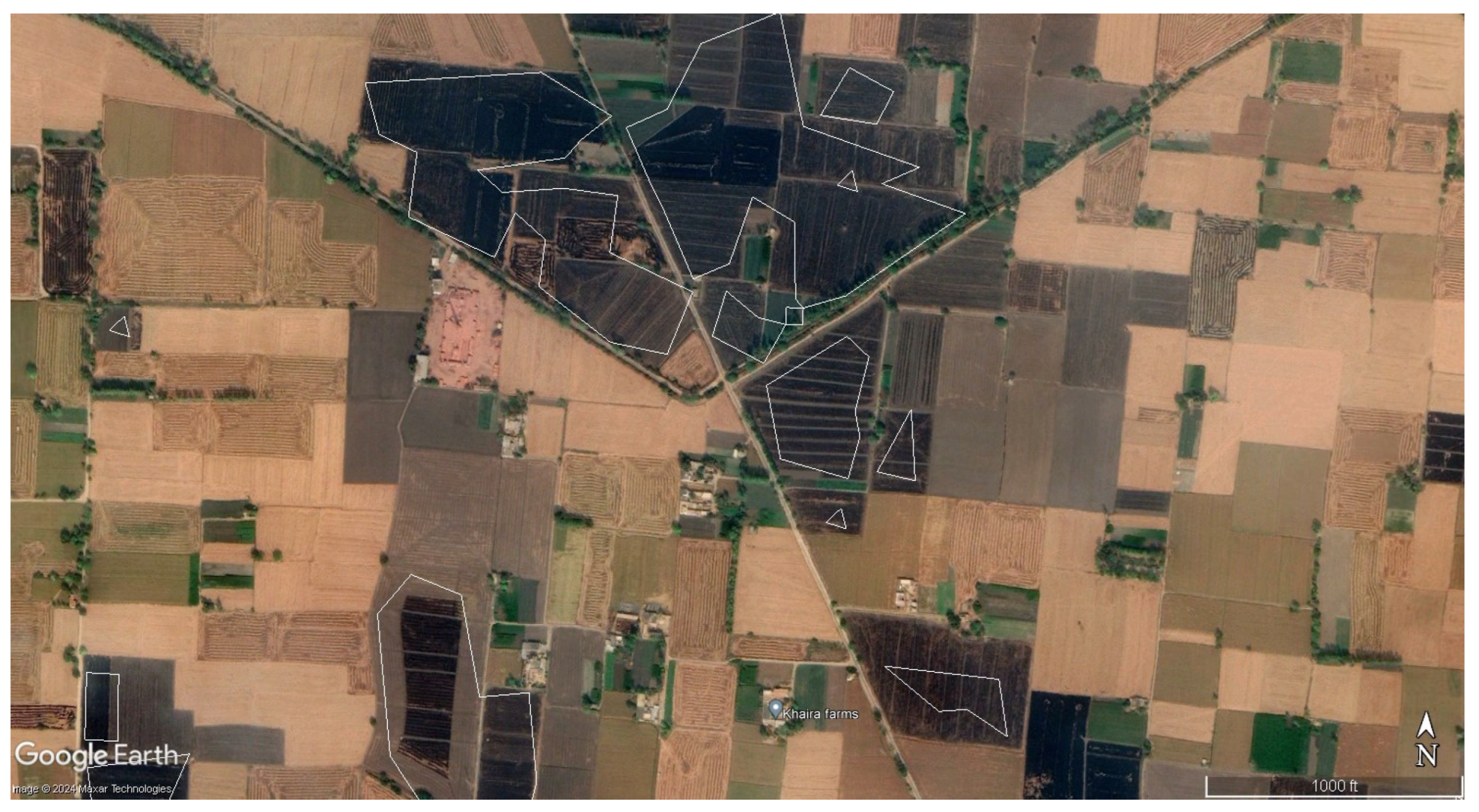
Figure 12.
On-ground validation sites in Punjab, India. Red circles show buffer zones with the presence of BA most likely detected using the model.
Figure 12.
On-ground validation sites in Punjab, India. Red circles show buffer zones with the presence of BA most likely detected using the model.
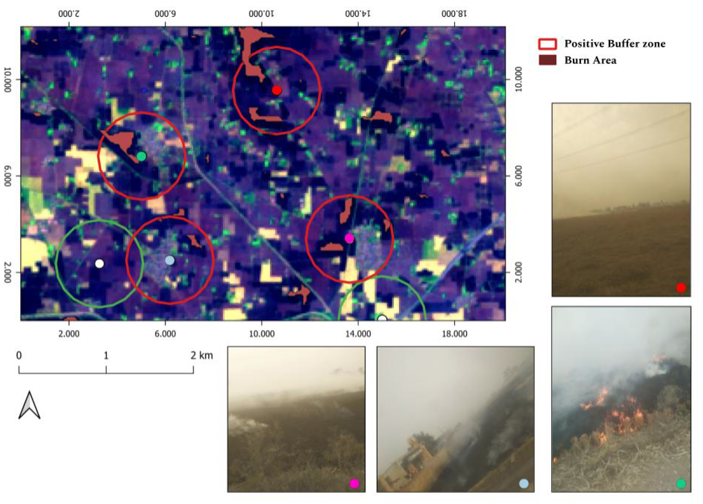
Figure 13.
Buffer zone analysis. Red spots signify burn areas.
Of the 94 sites, 27 showed strong evidence of burned areas detected within the 500 m buffer zone. Several factors contribute to this number. The survey images were captured during November 9–11, 2020, whereas the closest available Sentinel-2 images were taken on November 3 and 13, 2020. This timing discrepancy suggests that burning might have occurred either before or after the available satellite imagery, thereby affecting the validation accuracy. The positive observations from these 27 sites are important because they confirm the model’s capability to detect burned areas accurately in real-world scenarios. However, the lower number of positive validations can be attributed to the timing mismatch between ground truth data collection and satellite image acquisition. Despite these challenges, buffer zone analysis has been an important step in validating and refining our model, ensuring its reliability and effectiveness in real-world applications.
4.5. Spatiotemporal Distribution of Monthly Fire Activity for Post-Monsoon Burning Season (2020–2023))
As described in the preceding section, we performed an on-site survey to analyze the ground truth characteristics of the model in capturing small burn areas. However, given the limited number of on-site images and temporal gaps in Sentinel-2 observation, broader validation must be done to verify the model predictions comprehensively. We therefore compared the spatial distribution of burn areas in the form of monthly composites predicted using the fine-tuned model during the post-monsoon peak (October–November) from 2020–2023 with the MODIS-based MCD64A1 global burn area product. MCD64A1 is a global burn area product, integral to the Global Fire Emission Database (GFED, ver. 4), which combines 500 m resolution observations with 1 km MODIS active fire data. The burn area mapping algorithm uses a burn-sensitive vegetation index (VI) derived from shortwave infrared bands 5 and 7 [74]. Detailed information about the MCD64A1 algorithm is available in the literature [20]. Peak burning activity in both dataset is visible from late October to mid-November. [20].
Figure 14 and Figure 15 respectively portray the burn area distribution at the village level as detected using our DL model and MCD64A1 for the same period. Both the DL model and MCD64A1 identify a high-density burn area in northwest Punjab (Amritsar and the southern–central regions Taran Taran, Ferozpur) and the southern–central regions (Ludhiana, Barnala, Sangrur, Maler Kotla, Bhathinda) during October. This alignment underscores the model’s reliability in capturing the general burn area distribution. These observations are also consistent with high fire detection counts in southern districts reported by the [75] during an intensive observation campaign. Another study currently under review based on the Fire Detection Counts (FDC) by VIIRS S-NPP and PM 2.5 observations, [76] reported a continuous spike in FDC in Punjab from 2022 - 2021 and then observed a decline in FDC from 2022 - 2023. Both the DL model and MCD64A1 follow this trend of increasing FDC and show higher burning activity in 2020 and 2021. This increase can be attributed to the introduction of the Farmer’s Bill (Indian Agricultural Act), which led to excess crop residue burning by farmers. A decline in FDC during 2022–2023 is also observed in both the MCD64A1 and DL models. This decline matches a period of regulatory intervention, with stricter enforcement of residue management practices, as well as improvements in alternative farming methods [77].
It is noteworthy that the DL model excels in identifying small, fragmented burn patches that are often overlooked by coarser-resolution products like MCD64A1. This strength is particularly evident during periods of lower burning activity such as early October, where the DL model estimates at finer spatial scales, such as the village level, which could be crucially important for local-level policy interventions. Despite its benefits, the overall burn area detected by the DL model is markedly less than that of MCD64A1. This discrepancy can be attributed to the DL model’s current emphasis on small-scale fires, which, while complementary, might not account for larger, contiguous burn areas comprehensively. Additionally, factors such as temporal gaps in Sentinel-2, especially during periods of high cloud cover, contribute further to underestimation. Robust cloud and shadow masking techniques might mitigate this issue in future analyses [78].
This comparison provides a benchmark for evaluating the DL model’s performance against an established and widely used dataset, enabling us to assess its reliability in capturing both small-scale and regional burn area patterns. Additionally, this comparison provides insights into the complementary strengths of the two approaches while addressing the observed difference in all burned area estimates. The fine-tuned model demonstrates the ability to detect small and fragmented burn areas which are often missed by coarser-resolution products such as MCD64A1. For instance, during a period of lower burning activity, such as October 2022, the DL Model captures fine-grained details that provide a more localized understanding of burn area distributions.
The smaller total burned area detected using the DL model is not entirely a limitation of its core design, but rather reflects its specialized emphasis on small and fragmented fires. Factors such as temporal gaps and in Sentinel-2, especially during periods of high cloud cover, contribute further to underestimation. These findings highlight the complementary characteristics of the DL model. Whereas MCD64A1 captures the large-scale patterns effectively, the DL model adds value by filling the critical gaps in the detection of small and fragmented burn areas. This complementary approach could enhance fire emission inventories, such as the Fire Inventory from NCAR (FINN) [79] by integrating the MODIS, VIIRS, and Sentinel-2 observations for more accurate emission estimation.
4.6. Comparison with MCD64A1 Burn Area Product
This section presents comparison of the burn area distributions and trends captured by MCD64A1 and the DL model for the post-monsoon burning season (October–November). Despite large differences in the scales of burn areas captured by MCD64A1 and the DL model, both datasets generally align in capturing the temporal trends of burning during peak fire season, which gradually peaks from mid-October to mid-November. However, notable deviations are apparent, particularly at the beginning and end of the burning season, reflecting the DL model’s sensitivity for small and fragmented fires.
Figure 16.
Time series of burn area distribution by size for the DL model and MCD64A1.
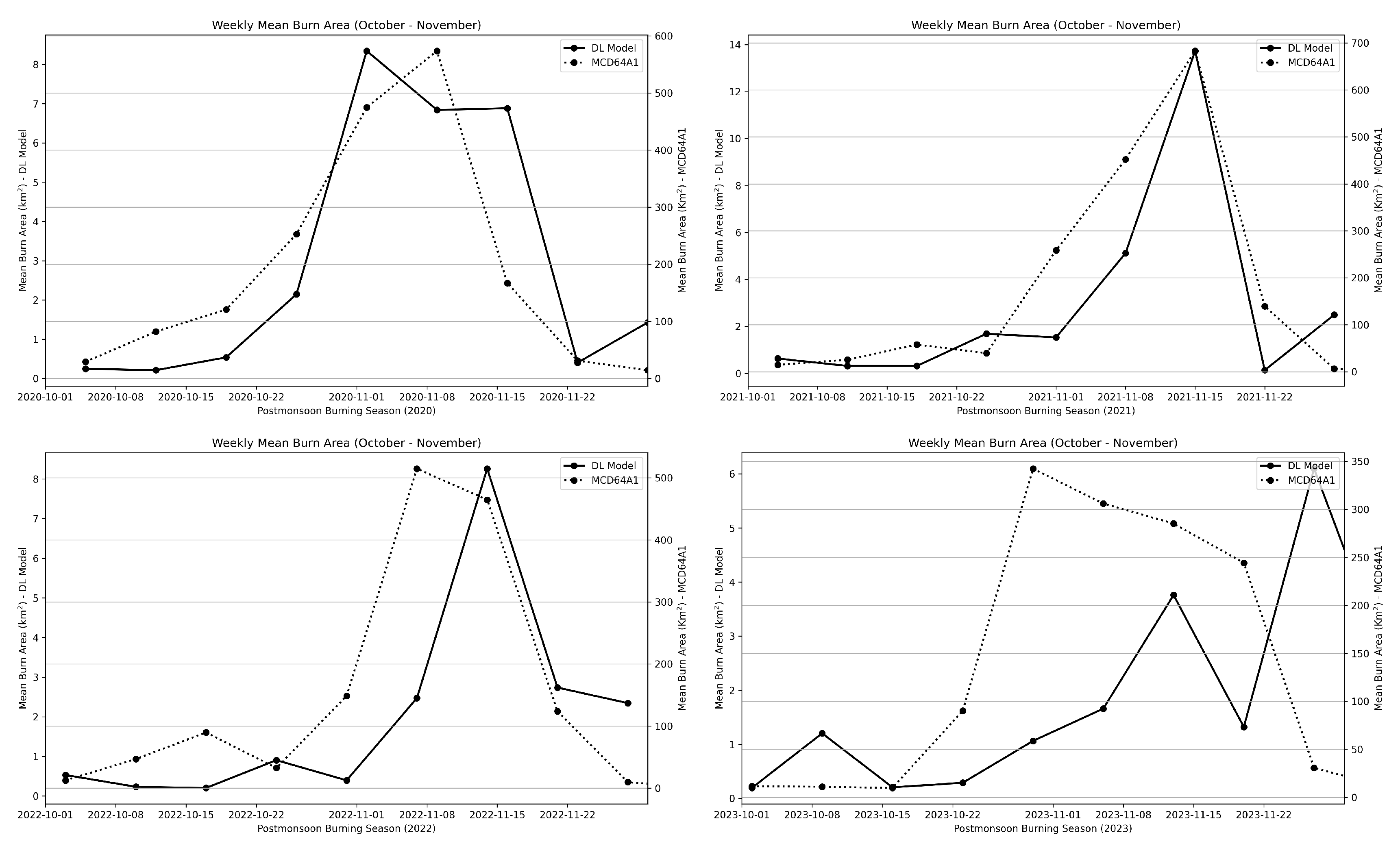
The peak captured by the DL model and MCD64A1 aligns closely during the peak burning season, particularly for the years 2020 and 2021. However, discrepancies exist especially at the tail of the season where DL models detect increased activity in early October and late November. This is likely attributable to its ability to identify smaller fires (<250 m2) that are often overlooked by MCD64A1 because of its coarser resolution and lower sensitivity. Actually, MCD64A1 has been reported to perform poorly in detecting fires smaller than (<250 ) that are often overlooked by MCD64A1 due to its coarser resolution and lower sensitivity. MCD64A1 dataset can capture fires up to 1000 under regular conditions and up to 50 under very clear, cloud-free conditions [11].
A recent study by [80] analyzed the degrees of spatial accuracy of several MODIS-based burn area products, including MCD64A1 and FireCCI51, against fire size. They reported that fires smaller than 250 ha (2.5 ) had Dice scores of 0.22 for MCD64A1 and 0.24 for FireCCI51. By contrast, the DL model achieves a Dice score of 0.64, for burn area size up to <250 . This advantage is particularly relevant for agricultural fields in Punjab, where small and fragmented fire dominates the post-harvest period. A summary of recent burn area algorithms and their respective accuracy can be found in Table 3. Additionally, other reasons for this deviation might be the temporal gap in Sentinel-2 observation and cloud cover interference. Another plausible explaination is that because the model was trained primarily on peak burning season data, it has not been exposed extensively to low or non-burning season conditions. This lack of diverse seasonal data might affect its performance, especially during transition periods.
Although MCD64A1 captures large-scale trends effectively, the DL model provides valuable insights into smaller fires, thereby enhancing the burn area mapping granularity. However, the DL model’s current limitations, and particularly its training focused on peak fire seasons, highlight the need for broader training datasets that include non-burning seasons. Addressing these gaps can improve its generalization across varying fire activity periods, reinforcing its utility for accurate agricultural fire monitoring.
4.7. Limitations
Although the fine-tuned model demonstrates a strong capability for delineating small agricultural burn areas with higher accuracy than that of the conventional method, several limitations should be acknowledged to provide perspective and highlight opportunities for future improvement. Regarding limitations of annotated data, the model’s performance is constrained by the limited availability of annotated training data. Because the annotation process is manual and time-intensive, the dataset size is small, which might have affected the model’s ability to be generalized effectively. Moreover, this limitation might contribute to underestimation of the total burned areas and a potential inability to capture the full scope of fires, as reflected in the observed discrepancy between the DL model and MCD64A1 estimates. Expanding the annotation dataset with diverse examples from different regions and fire seasons can enhance the model’s capability to represent the totality of fires accurately.
Regarding limited on-site validation, on-site surveys, although valuable for validating the model’s ability to capture small burn areas, are limited in scope to a small number of images collected and temporal gaps in the Sentinel-2. This limited scope restricted the ability to verify the model’s prediction on the ground. In terms of experimental design and applicability, the current experiment design marks a promising step towards leveraging deep learning for high-resolution burn area mapping, but it is not comprehensive. The model was trained explicitly using data from the post-monsoon peak burning season. For that reason, its performance in non-fire seasons or in regions with different patterns might be inadequate.
Spatial and temporal coverage, temporal coverage in this study is hindered by the Sentinel-2 satellite’s five-day revisit period. Given the sporadic characteristics of burning practices, some fire events are likely to be missed between observations. Integrating data from multiple satellites with different revisitation periods might help capture a more comprehensive picture of burn activity.
Also, regarding cloud interference, the model’s accuracy is affected by the presence of clouds and cloud shadows, which obscure burn area features in Sentinel-2 imagery. For instance, the reduced number of cloud-free tiles in October 2022 likely contributed to the lower burned area detection during this period. Applying robust cloud and shadow masking techniques [78] or integrating observation from other satellites with complementary temporal coverage such as Landsat or VIIRS might mitigate this issue. Gaps in burn area estimates using the DL model and MCD64A1 are problematic: the models specifically examine small and fragmented fires, inherently leading to lower total burned areas than those found using MCD64A1, which operates at a coarser resolution and which captures larger, contiguous fire events. With present capabilities, the DL model enhances, rather than replaces, global burn area products by addressing gaps in small fire detection.
5. Conclusion and Future Scope
This study highlights the effects of combining high-resolution Sentinel-2 imagery, a deep learning segmentation model, and transfer learning approaches for accurate mapping of small agricultural burn areas. Initially trained using data from Portugal, the model showed reliable capability for capturing large fires and for delineating burn areas. After fine-tuning was conducted using data from Punjab, the model’s ability to detect small burn patches in agricultural areas improved considerably. This enhanced accuracy is crucially important for quantifying the contributions of small fires to overall emissions. Additionally, the DL model exhibited superior burn area mapping efficiency compared to the baseline NBR index method. One salient benefit of this study is its promising methodology for assessing burn areas and their effects in regions with limited ground truth data. Furthermore, the model’s adaptability allows its application to detect burn areas in other similar agricultural regions worldwide. This study specifically addressed a single deep learning architecture, but future research might benefit from a comparative analysis of different neural networks in burn area mapping. Exploring advanced neural networks such as U-Net++, diffusion models, and one-shot learning might be particularly useful in scenarios with scarce data. Given the model’s accommodation of multiple datasets, integrating higher-resolution datasets such as Planetscope might provide burn area mapping that is even more precise. Additionally, further modifying the network architecture, especially during the transfer learning step, by adjusting the final layers of the neural network might enhance the overall model accuracy.
Author Contributions
Conceptualization, methodology: Anand Anamika and Imasu Ryoichi; software, data curation, analysis, validation, visualization: Anand Anamika; supervision, resources: Imasu Ryoichi; writing – original draft preparation: Anand Anamika; writing – review and editing: Anand Anamika, Dhaka Kumar Surendra, Imasu Ryoichi; project administration: Prabir Patra; All authors have read and agreed to the published version of the manuscript
Funding
This research was partially supported by Research Institute for Humanity and Nature (RIHN: a constituent member of NIHU) Project No. 14200133. This research was conducted using the computational resources of Fujitsu PRIMEHPC FX1000 and FUJITSU PRIMERGY GX2570 (Wisteria/BDEC-01) at the Information Technology Center, The University of Tokyo.
Acknowledgments
We are especially grateful to Dr. Tanbir Singh, Prof. Kamal Vatta, and Prof. Kanako Muramatsu for providing on-site images from the AAKASH project campaign. We express our heartfelt thanks to Ms. Lisa Knopp for her expertise and encouragement, which have been greatly appreciated. We have used Land Use Land Cover information related to our research work from the Natural Resources Census Project of the National Remote Sensing Centre (NRSC), ISRO, Hyderabad, India. Digital Database: Digital Database Bhuvan – Thematic Services, LULC503/MAP/PB.jpg, NRSC/ISRO – India.
Conflicts of Interest
The authors declare no conflicts of interest.
Abbreviations
The following abbreviations are used in this manuscript:
| DL | Deep Learning |
| CNN | Convolutional Neural Networks |
| NBR | Normalized Burn Ratio |
| MODIS | Moderate Resolution Imaging Spectroradiometer |
| VIIRS | Visible Infrared Imaging Radiometer Suite |
| NIR | Near Infrared |
| SWIR | Shortwave Infrared |
| ICNF | Institute for Nature Conservation and Forests |
| MSI | Multispectral Instrument |
| TOA | Top of Atmosphere |
| IoU | Intersection over Union |
| Ano1 | Annotation 1 |
| Ano2 | Annotation 2 |
| FDC | Fire Detection Counts |
Appendix A
Appendix A.1
Figure A1.
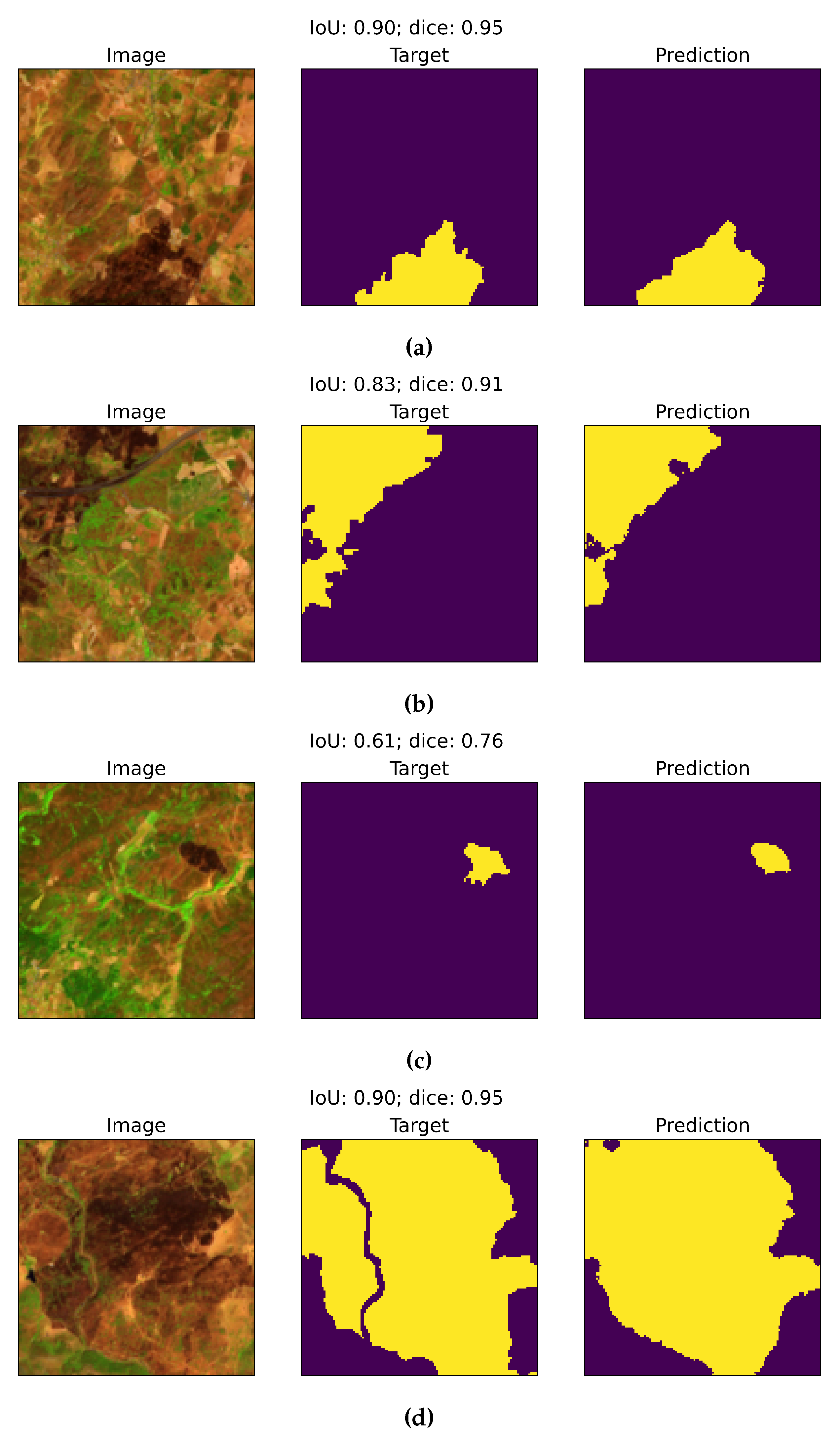
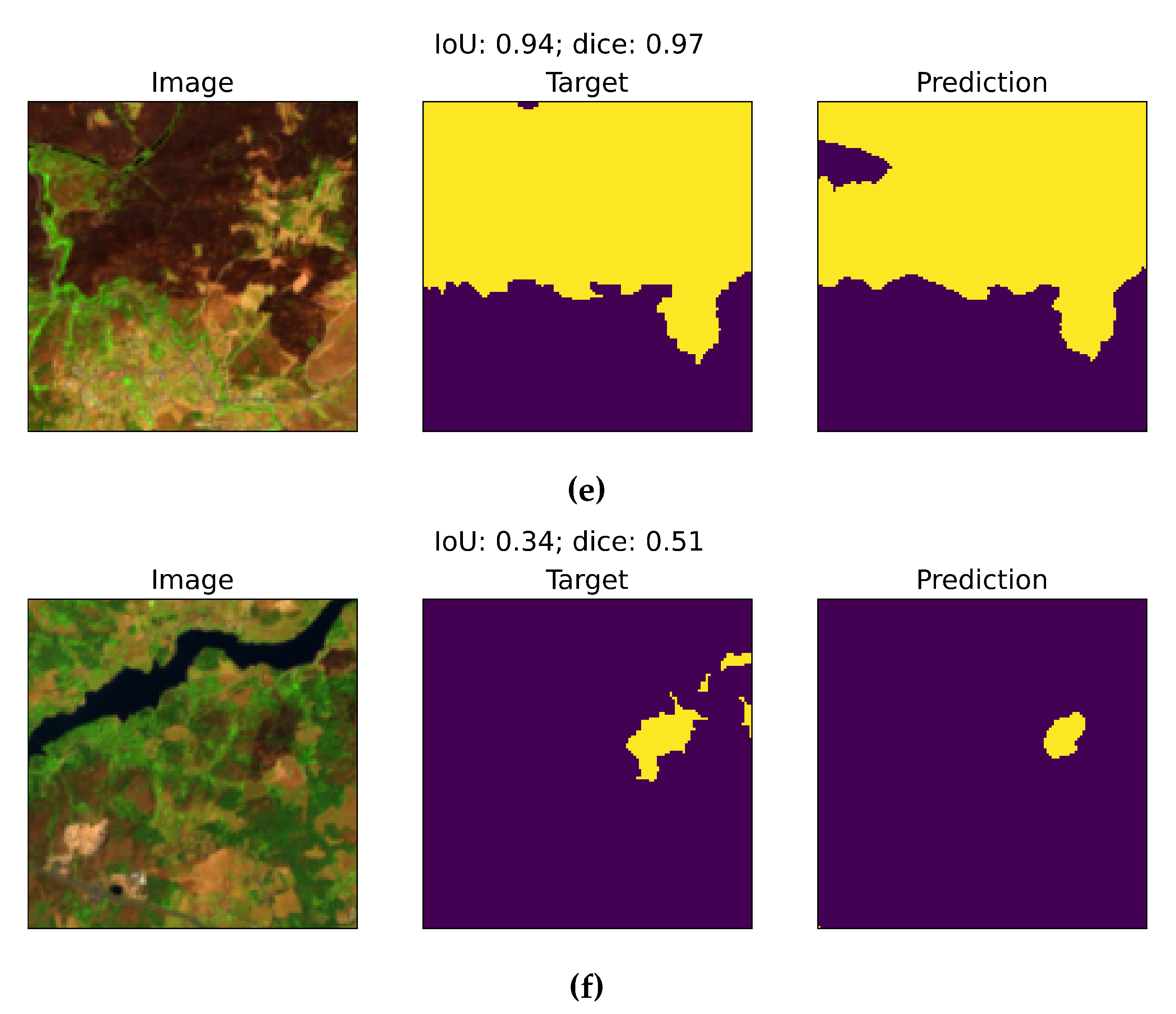
Left panels show Sentinel-2 false-color images (Green, NIR, and SWIR) over Portugal. Middle panels display ground truth data from ICNF. Right panels present model predictions. IoU and Dice scores quantify similarities between ground truth and the model output. Panels (a), (b), and (d) show high similarity and the model’s capability to capture the full extent of large fires. Panel (c) shows the detection of a small fire with high similarity in unburned areas. Panel (e) highlights a potential error in the ground truth data, but the model accurately identifies unburned areas. Panel (f) presents the model’s difficulty in capturing some small burn patches, leading to lower IoU and Dice scores, although it detects large fires with some fragmentation.
Figure A1.
Left panels show Sentinel-2 false-color images (Green, NIR, and SWIR) over Portugal. Middle panels display ground truth data from ICNF. Right panels present model predictions. IoU and Dice scores quantify similarities between ground truth and the model output. Panels (a), (b), and (d) show high similarity and the model’s capability to capture the full extent of large fires. Panel (c) shows the detection of a small fire with high similarity in unburned areas. Panel (e) highlights a potential error in the ground truth data, but the model accurately identifies unburned areas. Panel (f) presents the model’s difficulty in capturing some small burn patches, leading to lower IoU and Dice scores, although it detects large fires with some fragmentation.
Appendix B Experimental Details:
The first phase included Experiments A and B. For Experiment A, a raw CNN network was trained over Portugal using data of 2016. For Experiment B, the network was trained further using more data from 2017. Our goal in this effort was to reproduce similar degrees of accuracy to those of an experiment conducted for an earlier study [37]. This step was crucially important to imbue the model with a general capability to segment burned and unburned areas. The second phase involved numerous experiments with the aim of monitoring the sensitivity and precision over detection of small burn areas. Experiment C involved direct application of transfer learning to the pretrained model to assess how well the pretrained model can capture burn areas over Punjab.
Experiment D involved fine tuning of the pretrained model over Portugal using the first set of hand-annotated data over Punjab, where the learning rate was reduced to 0.0003, whereas other parameters were left at their default values. For Experiment E, the batch size was reduced to 16 to assess its effects on model accuracy, particularly addressing small delineations of burned areas. For Experiment F, the batch size was reduced further to 8 whereas other parameters were kept the same.
For Experiment G, we used model weights from experiment E and a second set of annotation data (Ano 2). For Experiment H, we used model weights from Experiment B and both sets of annotation data together (Ano1 and Ano2). For Experiments I–K, all hyperparameters were kept at default values. For Experiment I, we used model weights from Experiment B and the first set of annotation data (Ano 1), froze the layers of encoder for the 25 epochs, and unfroze the last layer of the encoder and ran fine tuning for another 5 epochs. For Experiment J, we also used the model weights from Experiment B and Ano1 data. The encoder layers were kept frozen for all 30 epochs.
Experiment K was identical to Experiment J, except that Ano2 was used as the input data. For the Experiment L, we used the model weights from Experiment B and used Ano1 as an input and trained model with 45 epochs where the encoder layers were kept frozen for 15 epochs followed by unfreezing of the last layer and retraining of the whole network for another 25 epochs. For the final Experiment M, we used the model weights from Experiment L and used Ano2 as an input. The model was trained for a total of 40 epochs, where the encoder layers were kept frozen for the first 15 epochs, with subsequent unfreezing of the last layer and training of the whole network for the remaining 25 epochs.
The main goal of running the experiment in different phases and conditions was to monitor the transferability of learned features, effectiveness at capturing the boundaries of small fires, the ability to distinguish between aquatic and burned areas, and sensitivity toward other diverse features in the classification process. Earlier studies have demonstrated that such sequential fine-tuning improves hierarchical feature learning and enhances accuracy in diverse domains [82]. This entire process enables us to explore different training configurations and their effects on model performance, leading to an optimized approach for burned area detection. Details of all the experiments summarized above are presented in Table A1.
Table A1.
Comprehensive overview of all experiments conducted, highlighting the different stages, conditions, and key parameters modified during training
Table A1.
Comprehensive overview of all experiments conducted, highlighting the different stages, conditions, and key parameters modified during training
| Expt. | Descr. | Domain | GT-Data | lr | batch size | w | Encoder layers | Epochs |
|---|---|---|---|---|---|---|---|---|
| A | raw model | Portugal (2016) | ICNF | 0.0003 | 32 | 0.0001 | unfrozen | 50 |
| B | Pretrained | Portugal (2017) | ICNF | 0.0003 | 32 | 0.0001 | unfrozen | 50 |
| C | Pretrained | Punjab (2020) | ICNF | 0.0003 | 32 | 0.0001 | unfrozen | 60 |
| D | TL-Pretrained | Punjab (2020) | Ano 1 | 3E-5 | 32 | 0.0001 | unfrozen | 60 |
| E | TL-Pretrained | Punjab (2020) | Ano 1 | 0.0003 | 16 | 0.0001 | unfrozen | 50 |
| F | TL-Pretrained | Punjab (2020) | Ano 1 | 0.0003 | 8 | 0.0001 | unfrozen | 50 |
| G | TL-Pretrained | Punjab (2020) | Ano 2 | 0.0003 | 16 | 0.0001 | unfrozen | 45 |
| H | TL-Pretrained | Punjab (2020) |
Ano 1 + Ano 2 |
0.0003 | 16 | 0.0001 | unfrozen | 60 |
| I | TL-Pretrained | Punjab (2020) | Ano 1 | 0.0003 | 16 | 0.001 | frozen | 25 + 5* |
| J | TL-Pretrained | Punjab (2020) | Ano 1 | 0.0003 | 16 | 0.001 | frozen | 30 |
| K | TL-Pretrained | Punjab (2020) | Ano 2 | 0.0003 | 16 | 0.001 | frozen | 30 |
| L | TL-Pretrained | Punjab (2020) | Ano 1 | 0.0003 | 16 | 0.001 | frozen | 15 + 30* |
| M | TL-Pretrained | Punjab (2020) | Ano 2 | 0.0003 | 16 | 0.001 | frozen | 15 + 25* |
Note: * The last layer of the encoder was unfrozen. The whole network was retrained. For example, 25+5* signifies that the encoder layers were frozen for 25 epochs, that the last layer was unfrozen, and that the whole network was retrained for 5 additional epochs.
Table A2.
Performance metrics for Experiments A–M conducted using different models and datasets
| Experiment | Domain | Type | Metric | Burned (%) | Non-burned (%) |
| Precision | 81.6 | 96.7 | |||
| Class | Recall | 80.9 | 96.9 | ||
| A | Portugal | F1 | 81.2 | 96.8 | |
| Accuracy (%) | 94.5 | ||||
| Overall | Macro-F1 (%) | 89 | |||
| IoU | 0.52 | ||||
| Dice | 0.60 | ||||
| Precision | 90.5 | 97.9 | |||
| Class | Recall | 87.8 | 98.5 | ||
| B | Punjab | F1 | 89.1 | 98.2 | |
| Accuracy (%) | 96.9 | ||||
| Overall | Macro-F1 (%) | 93.7 | |||
| IoU | 0.54 | ||||
| Dice | 0.64 | ||||
| Precision | 95.1 | 99 | |||
| Class | Recall | 94.9 | 99.1 | ||
| C | Punjab | F1 | 94.8 | 99.0 | |
| Accuracy (%) | 98.4 | ||||
| Overall | Macro-F1 (%) | 95.0 | |||
| IoU | 0.10 | ||||
| Dice | 0.13 | ||||
| Precision | 95 | 99 | |||
| Class | Recall | 94 | 99 | ||
| D | Punjab | F1 | 94 | 99 | |
| Accuracy (%) | 98.3 | ||||
| Overall | Macro-F1 (%) | 97 | |||
| IoU | 0.44 | ||||
| Dice | 0.60 | ||||
| Precision | 95.1 | 99 | |||
| Class | Recall | 94.5 | 99.1 | ||
| E | Punjab | F1 | 94 | 99 | |
| Accuracy (%) | 98.1 | ||||
| Overall | Macro-F1 (%) | 97 | |||
| IoU | 0.45 | ||||
| Dice | 0.60 | ||||
| Precision | 95 | 99 | |||
| Class | Recall | 94 | 99 | ||
| F | Punjab | F1 | 94 | 99 | |
| Accuracy (%) | 99 | ||||
| Overall | Macro-F1 (%) | 97.1 | |||
| IoU | 0.46 | ||||
| Dice | 0.61 | ||||
| Precision | 95.4 | 99.1 | |||
| Class | Recall | 95.3 | 99.1 | ||
| G | Punjab | F1 | 95.3 | 99.08 | |
| Accuracy (%) | 98.4 | ||||
| Overall | Macro-F1 (%) | 97.2 | |||
| IoU | 0.52 | ||||
| Dice | 0.64 | ||||
| Precision | 95.1 | 98.9 | |||
| Class | Recall | 94.4 | 99 | ||
| H | Punjab | F1 | 94.7 | 98.6 | |
| Accuracy (%) | 98.7 | ||||
| Overall | Macro-F1 (%) | 96.8 | |||
| IoU | 0.42 | ||||
| Dice | 0.54 | ||||
| Precision | 95 | 99.1 | |||
| Class | Recall | 95.2 | 99 | ||
| I | Punjab | F1 | 95.1 | 99.1 | |
| Accuracy (%) | 98.4 | ||||
| Overall | Macro-F1 (%) | 97 | |||
| IoU | 0.39 | ||||
| Dice | 0.54 | ||||
| Precision | 95.1 | 99 | |||
| Class | Recall | 94.7 | 99.1 | ||
| J | Punjab | F1 | 94.9 | 99 | |
| Accuracy (%) | 98.3 | ||||
| Overall | Macro-F1 (%) | 96.9 | |||
| IoU | 0.43 | ||||
| Dice | 0.59 | ||||
| Precision | 96 | 99.2 | |||
| Class | Recall | 95.7 | 99.2 | ||
| K | Punjab | F1 | 95.9 | 99.2 | |
| Accuracy (%) | 98.6 | ||||
| Overall | Macro-F1 (%) | 97.5 | |||
| IoU | 0.48 | ||||
| Dice | 0.58 | ||||
| Precision | 95.1 | 99 | |||
| Class | Recall | 95 | 99.1 | ||
| L | Punjab | F1 | 95 | 99 | |
| Accuracy (%) | 98.4 | ||||
| Overall | Macro-F1 (%) | 97 | |||
| IoU | 0.43 | ||||
| Dice | 0.58 | ||||
| Precision | 96 | 98.2 | |||
| Class | Recall | 95.8 | 99.2 | ||
| M | Punjab | F1 | 95.9 | 99.2 | |
| Accuracy (%) | 98.7 | ||||
| Overall | Macro-F1 (%) | 97.6 | |||
| IoU | 0.54 | ||||
| Dice | 0.64 | ||||
Table A3.
Model segmentation accuracy for all experiments using test and validation data
| Phase | Expt. | Domain | IoU (Val) | Dice (Val) | Model Accuracy IoU (Test) |
Dice (Test) |
Val_loss | Train_loss |
|---|---|---|---|---|---|---|---|---|
| I | A | Portugal | 0.62 | 0.72 | 0.50 | 0.59 | 0.34 | 0.33 |
| B | Portugal | 0.66 | 0.75 | 0.52 | 0.60 | 0.33 | 0.32 | |
| II | C | Punjab | 0.10 | 0.13 | ||||
| D | Punjab | 0.44 | 0.60 | 0.45 | 0.60 | 0.42 | 0.42 | |
| E | Punjab | 0.48 | 0.64 | 0.45 | 0.60 | 0.38 | 0.38 | |
| F | Punjab | 0.49 | 0.64 | 0.46 | 0.61 | 0.38 | 0.37 | |
| G | Punjab | 0.49 | 0.60 | 0.52 | 0.64 | 0.51 | 0.43 | |
| H | Punjab | 0.40 | 0.53 | 0.42 | 0.54 | 0.45 | 0.40 | |
| I | Punjab | 0.40 | 0.55 | 0.39 | 0.54 | 0.44 | 0.51 | |
| J | Punjab | 0.44 | 0.59 | 0.43 | 0.59 | 0.48 | 0.49 | |
| K | Punjab | 0.47 | 0.57 | 0.48 | 0.58 | 0.58 | 0.56 | |
| L | Punjab | 0.43 | 0.59 | 0.43 | 0.58 | 0.44 | 0.45 | |
| M | Punjab | 0.49 | 0.60 | 0.54 | 0.64 | 0.56 | 0.51 |
References
- Korontzi, S.; McCarty, J.; Loboda, T.; Kumar, S.; Justice, C. Global distribution of agricultural fires in croplands from 3 years of Moderate Resolution Imaging Spectroradiometer (MODIS) data. Global Biogeochemical Cycles - GLOBAL BIOGEOCHEM CYCLE 2006, 20. [Google Scholar] [CrossRef]
- Cassou, E. Field Burning. Technical report, World Bank, Washington, DC, 2018. [CrossRef]
- Kumar, P.; Kumar, S.; Joshi, L. The Extent and Management of Crop Stubble. In Socioeconomic and Environmental Implications of Agricultural Residue Burning: A Case Study of Punjab, India; Springer: New Delhi, India, 2015; pp. 13–34. [Google Scholar] [CrossRef]
- Jethva, H.; Torres, O.; Field, R.D.; Lyapustin, A.; Gautam, R.; Kayetha, V. Connecting Crop Productivity, Residue Fires, and Air Quality over Northern India. Scientific Reports 2019, 9. [Google Scholar] [CrossRef]
- Deshpande, M.V.; Kumar, N.; Pillai, D.; Krishna, V.V.; Jain, M. Greenhouse gas emissions from agricultural residue burning have increased by 75% since 2011 across India. Science of The Total Environment 2023, 904, 166944. [Google Scholar] [CrossRef] [PubMed]
- van der Werf, G.R.; Randerson, J.T.; Giglio, L.; Collatz, G.J.; Mu, M.; Kasibhatla, P.S.; Morton, D.C.; DeFries, R.S.; Jin, Y.; van Leeuwen, T.T. Global fire emissions and the contribution of deforestation, savanna, forest, agricultural, and peat fires (1997–2009). Atmospheric Chemistry and Physics 2010, 10, 11707–11735. [Google Scholar] [CrossRef]
- Singh, R.; Sinha, B.; Hakkim, H.; Sinha, V. Source apportionment of volatile organic compounds during paddy-residue burning season in north-west India reveals large pool of photochemically formed air toxics. Environmental Pollution 2023, 338, 122656. [Google Scholar] [CrossRef]
- Dhaka, S.K.; Chetna.; Kumar, V.; Panwar, V.; Dimri, A.; Singh, N.; Patra, P.K.; Matsumi, Y.; Takigawa, M.; Nakayama, T.; et al. PM2. 5 diminution and haze events over Delhi during the COVID-19 lockdown period: an interplay between the baseline pollution and meteorology. Scientific reports 2020, 10, 13442.
- Hall, J.V.; Loboda, T.V. Quantifying the Potential for Low-Level Transport of Black Carbon Emissions from Cropland Burning in Russia to the Snow-Covered Arctic. Frontiers in Earth Science 2017, 5. [Google Scholar] [CrossRef]
- Andreae, M.O. Biomass Burning: Its History, Use, and Distribution and Its Impact on Environmental Quality and Global Climate. In Global Biomass Burning; The MIT Press, 1991; p. 3–21. [CrossRef]
- Hall, J.V.; Loboda, T.V.; Giglio, L.; McCarty, G.W. A MODIS-based burned area assessment for Russian croplands: Mapping requirements and challenges. Remote Sensing of Environment 2016, 184, 506–521. [Google Scholar] [CrossRef]
- Seiler, W.; Crutzen, P.J. Estimates of gross and net fluxes of carbon between the biosphere and the atmosphere from biomass burning. Climatic change 1980, 2, 207–247. [Google Scholar] [CrossRef]
- Van Der Werf, G.R.; Randerson, J.T.; Giglio, L.; Gobron, N.; Dolman, A. Climate controls on the variability of fires in the tropics and subtropics. Global Biogeochemical Cycles 2008, 22. [Google Scholar] [CrossRef]
- Ramo, R.; Roteta, E.; Bistinas, I.; Van Wees, D.; Bastarrika, A.; Chuvieco, E.; Van der Werf, G.R. African burned area and fire carbon emissions are strongly impacted by small fires undetected by coarse resolution satellite data. Proceedings of the National Academy of Sciences 2021, 118, e2011160118. [Google Scholar] [CrossRef]
- Andela, N.; Morton, D.C.; Giglio, L.; Paugam, R.; Chen, Y.; Hantson, S.; Van Der Werf, G.R.; Randerson, J.T. The Global Fire Atlas of individual fire size, duration, speed and direction. Earth System Science Data 2019, 11, 529–552. [Google Scholar] [CrossRef]
- Konovalov, I.; Beekmann, M.; Kuznetsova, I.N.; Yurova, A.; Zvyagintsev, A. Atmospheric impacts of the 2010 Russian wildfires: integrating modelling and measurements of an extreme air pollution episode in the Moscow region. Atmospheric Chemistry and Physics 2011, 11, 10031–10056. [Google Scholar] [CrossRef]
- Archibald, S.; Lehmann, C.E.; Gómez-Dans, J.L.; Bradstock, R.A. Defining pyromes and global syndromes of fire regimes. Proceedings of the National Academy of Sciences 2013, 110, 6442–6447. [Google Scholar] [CrossRef] [PubMed]
- Chuvieco, E.; Mouillot, F.; van der Werf, G.R.; San Miguel, J.; Tanase, M.; Koutsias, N.; García, M.; Yebra, M.; Padilla, M.; Gitas, I.; et al. Historical background and current developments for mapping burned area from satellite Earth observation. Remote Sensing of Environment 2019, 225, 45–64. [Google Scholar] [CrossRef]
- GCOS. The global observing system for climate: Implementation needs. World Meteorol. Organ. 2016, 200, 316. [Google Scholar]
- Giglio, L.; Boschetti, L.; Roy, D.P.; Humber, M.L.; Justice, C.O. The Collection 6 MODIS burned area mapping algorithm and product. Remote Sensing of Environment 2018, 217, 72–85. [Google Scholar] [CrossRef] [PubMed]
- Roteta, E.; Bastarrika, A.; Padilla, M.; Storm, T.; Chuvieco, E. Development of a Sentinel-2 burned area algorithm: Generation of a small fire database for sub-Saharan Africa. Remote Sensing of Environment 2019, 222, 1–17. [Google Scholar] [CrossRef]
- Roy, D.P.; Boschetti, L. Southern Africa validation of the MODIS, L3JRC, and GlobCarbon burned-area products. IEEE transactions on Geoscience and Remote Sensing 2009, 47, 1032–1044. [Google Scholar] [CrossRef]
- Roy, D.; Boschetti, L.; Justice, C.; Ju, J. The collection 5 MODIS burned area product — Global evaluation by comparison with the MODIS active fire product. Remote Sensing of Environment 2008, 112, 3690–3707. [Google Scholar] [CrossRef]
- Giglio, L.; Loboda, T.; Roy, D.P.; Quayle, B.; Justice, C.O. An active-fire based burned area mapping algorithm for the MODIS sensor. Remote Sensing of Environment 2009, 113, 408–420. [Google Scholar] [CrossRef]
- L. Giglio, J.D.K.; Mack, R. A multi-year active fire dataset for the tropics derived from the TRMM VIRS. International Journal of Remote Sensing 2003, 24, 4505–4525. [Google Scholar] [CrossRef]
- McCarty, J.L.; Korontzi, S.; Justice, C.O.; Loboda, T. The spatial and temporal distribution of crop residue burning in the contiguous United States. Science of the Total Environment 2009, 407, 5701–5712. [Google Scholar] [CrossRef]
- Ouattara, B.; Thiel, M.; Sponholz, B.; Paeth, H.; Yebra, M.; Mouillot, F.; Kacic, P.; Hackman, K. Enhancing burned area monitoring with VIIRS dataset: A case study in Sub-Saharan Africa. Science of Remote Sensing 2024, 10, 100165. [Google Scholar] [CrossRef]
- Giglio, L.; Boschetti, L.; Roy, D.; Hoffmann, A.A.; Humber, M.; Hall, J.V. Collection 6 modis burned area product user’s guide version 1.0. NASA EOSDIS Land Processes DAAC: Sioux Falls, SD, USA.
- K. R. Al-Rawi, J.L.C.; Calle, A. Burned area mapping system and fire detection system, based on neural networks and NOAA-AVHRR imagery. International Journal of Remote Sensing 2001, 22, 2015–2032. [CrossRef]
- P. A. Brivio, M. Maggi, E.B.; Gallo, I. Mapping burned surfaces in Sub-Saharan Africa based on multi-temporal neural classification. International Journal of Remote Sensing 2003, 24, 4003–4016. [CrossRef]
- Wieland, M.; Li, Y.; Martinis, S. Multi-sensor cloud and cloud shadow segmentation with a convolutional neural network. Remote Sensing of Environment 2019, 230, 111203. [Google Scholar] [CrossRef]
- Wieland, M.; Martinis, S.; Kiefl, R.; Gstaiger, V. Semantic segmentation of water bodies in very high-resolution satellite and aerial images. Remote Sensing of Environment 2023, 287, 113452. [Google Scholar] [CrossRef]
- Maggiori, E.; Tarabalka, Y.; Charpiat, G.; Alliez, P. Convolutional Neural Networks for Large-Scale Remote-Sensing Image Classification. IEEE Transactions on Geoscience and Remote Sensing 2017, 55, 645–657. [Google Scholar] [CrossRef]
- Rustowicz, R.; Cheong, R.; Wang, L.; Ermon, S.; Burke, M.; Lobell, D. Semantic Segmentation of Crop Type in Africa: A Novel Dataset and Analysis of Deep Learning Methods. In Proceedings of the CVPR Workshops; 2019. [Google Scholar]
- Pinto, M.M.; Trigo, R.M.; Trigo, I.F.; DaCamara, C.C. A Practical Method for High-Resolution Burned Area Monitoring Using Sentinel-2 and VIIRS. Remote Sensing 2021, 13. [Google Scholar] [CrossRef]
- Knopp, L.; Wieland, M.; Rättich, M.; Martinis, S. A Deep Learning Approach for Burned Area Segmentation with Sentinel-2 Data. Remote Sensing 2020, 12. [Google Scholar] [CrossRef]
- Huppertz, R.; Nakalembe, C.; Kerner, H.; Lachyan, R.; Rischard, M. A: transfer learning to study burned area dynamics, 2021; arXiv:cs.LG/2107.14372].
- National Remote Sensing Centre (NRSC), ISRO. Land Use Land Cover Digital Database. https://bhuvan-app1.nrsc.gov.in/2dresources/thematic/LULC503/MAP/PB.jpg, 2024. Natural Resources Census Project, accessed 2024.
- Kumar, R.; Barth, M.; Pfister, G.; Nair, V.; Ghude, S.D.; Ojha, N. What controls the seasonal cycle of black carbon aerosols in India? Journal of Geophysical Research: Atmospheres 2015, 120, 7788–7812. [Google Scholar] [CrossRef]
- Kaskaoutis, D.; Kumar, S.; Sharma, D.; Singh, R.P.; Kharol, S.; Sharma, M.; Singh, A.; Singh, S.; Singh, A.; Singh, D. Effects of crop residue burning on aerosol properties, plume characteristics, and long-range transport over northern India. Journal of Geophysical Research: Atmospheres 2014, 119, 5424–5444. [Google Scholar] [CrossRef]
- Ravindra, K.; Singh, T.; Mor, S. Emissions of air pollutants from primary crop residue burning in India and their mitigation strategies for cleaner emissions. Journal of Cleaner Production 2019, 208, 261–273. [Google Scholar] [CrossRef]
- Chetna, N.; Devi, M.; et al. Forecasting of Pre-harvest Wheat Yield using Discriminant Function Analysis of Meteorological Parameters of Kurukshetra District of Haryana. Journal of Agriculture Research and Technology 2022, 47, 67–72. [Google Scholar] [CrossRef]
- Wang, J.; Christopher, S.A.; Nair, U.S.; Reid, J.S.; Prins, E.M.; Szykman, J.; Hand, J.L. Mesoscale modeling of Central American smoke transport to the United States: 1. “Top-down” assessment of emission strength and diurnal variation impacts. Journal of Geophysical Research: Atmospheres 2006, 111. [Google Scholar] [CrossRef]
- Sharma, A.R.; Kharol, S.K.; Badarinath, K.V.S.; Singh, D. Impact of agriculture crop residue burning on atmospheric aerosol loading – a study over Punjab State, India. Annales Geophysicae 2010, 28, 367–379. [Google Scholar] [CrossRef]
- Ronneberger, O.; Fischer, P.; Brox, T. U-Net: Convolutional Networks for Biomedical Image Segmentation. In Proceedings of the Medical Image Computing and Computer-Assisted Intervention – MICCAI 2015; Navab, N.; Hornegger, J.; Wells, W.M.; Frangi, A.F., Eds., Cham; 2015; pp. 234–241. [Google Scholar]
- Main-Knorn, M.; Pflug, B.; Louis, J.; Debaecker, V.; Müller-Wilm, U.; Gascon, F. Sen2Cor for Sentinel-2. In Proceedings of the Image and Signal Processing for Remote Sensing XXIII; Bruzzone, L., Ed. International Society for Optics and Photonics, SPIE, Vol. 10427; 2017; p. 1042704. [Google Scholar] [CrossRef]
- Sentinel-2 ESA’s Optical High-Resolution Mission for GMES Operational Services (ESA SP-1322/2 March 2012). Available online: https://sentinel.esa.int/documents/247904/349490/S2_SP-1322_2.pdf (accessed on 4 August 2024).
- Turco, M.; Jerez, S.; Augusto, S.; Tarín-Carrasco, P.; Ratola, N.; Jiménez-Guerrero, P.; Trigo, R.M. Climate drivers of the 2017 devastating fires in Portugal. Scientific Reports 2019, 9. [Google Scholar] [CrossRef] [PubMed]
- Menezes, L.S.; Russo, A.; Libonati, R.; Trigo, R.M.; Pereira, J.M.; Benali, A.; Ramos, A.M.; Gouveia, C.M.; Morales Rodriguez, C.A.; Deus, R. Lightning-induced fire regime in Portugal based on satellite-derived and in situ data. Agricultural and Forest Meteorology 2024, 355, 110108. [Google Scholar] [CrossRef]
- Copernicus Data Space Ecosystem - API - OData. Available online: https://documentation.dataspace.copernicus.eu/APIs/OData.html (accessed on 2 August 2024).
- Institute of Conservation of Nature and Forest. Available online: https://sig.icnf.pt/portal/home/item.html?id=983c4e6c4d5b4666b258a3ad5f3ea5af#overview (accessed on 2 August 2024).
- Vadrevu, K.; Lasko, K. Intercomparison of MODIS AQUA and VIIRS I-Band Fires and Emissions in an Agricultural Landscape—Implications for Air Pollution Research. Remote Sensing 2018, 10. [Google Scholar] [CrossRef]
- Liu, T.; Marlier, M.E.; Karambelas, A.; Jain, M.; Singh, S.; Singh, M.K.; Gautam, R.; DeFries, R.S. Missing emissions from post-monsoon agricultural fires in northwestern India: regional limitations of MODIS burned area and active fire products. Environmental Research Communications 2019, 1, 011007. [Google Scholar] [CrossRef]
- Key, C.; Benson, N. Measuring and remote sensing of burn severity. In Proceedings of the Joint Fire Science Conference and Workshop Proceedings: `Crossing the Millennium: Integrating Spatial Technologies and Ecological Principles for a New Age in Fire Management’, June 1999. [Google Scholar]
- Keeley, J. Fire intensity, fire severity and burn severity: A brief review and suggested usage. International Journal of Wildland Fire 2009, 18, 116–126. [Google Scholar] [CrossRef]
- He, K.; Zhang, X.; Ren, S.; Sun, J. Deep Residual Learning for Image Recognition. In Proceedings of the 2016 IEEE Conference on Computer Vision and Pattern Recognition (CVPR); 2016; pp. 770–778. [Google Scholar] [CrossRef]
- Zhao, H.; Shi, J.; Qi, X.; Wang, X.; Jia, J. Pyramid Scene Parsing Network. In Proceedings of the 2017 IEEE Conference on Computer Vision and Pattern Recognition (CVPR); 2017; pp. 6230–6239. [Google Scholar] [CrossRef]
- He, F.; Liu, T.; Tao, D. Control batch size and learning rate to generalize well: Theoretical and empirical evidence. Advances in neural information processing systems 2019, 32. [Google Scholar]
- Kingma, D.P.; Ba, J. Adam: A Method for Stochastic Optimization. In Proceedings of the 3rd International Conference on Learning Representations, ICLR 2015, San Diego, CA, USA, 2015, Conference Track Proceedings; Bengio, Y.; LeCun, Y., Eds., 2015., May 7-9.
- Ruby, U.; Yendapalli, V. Binary cross entropy with deep learning technique for image classification. Int. J. Adv. Trends Comput. Sci. Eng 2020, 9. [Google Scholar]
- Wisteria/BDEC-01 Supercomputer System. Available online: https://www.cc.u-tokyo.ac.jp/en/supercomputer/wisteria/service/ (accessed on 3 August 2024).
- Pereira, P.; Silveira, M. Cross-Modal Transfer Learning Methods for Alzheimer’s Disease Diagnosis. In Proceedings of the 2022 44th Annual International Conference of the IEEE Engineering in Medicine &, 2022, Biology Society (EMBC). IEEE; pp. 3789–3792.
- Garcia-Garcia, A.; Orts-Escolano, S.; Oprea, S.; Villena-Martinez, V.; Garcia-Rodriguez, J. A Review on Deep Learning Techniques Applied to Semantic Segmentation. arXiv, 2017; arXiv:cs.CV/1704.06857. [Google Scholar]
- Zou, K.H.; Warfield, S.K.; Bharatha, A.; Tempany, C.M.; Kaus, M.R.; Haker, S.J.; Wells, W.M.; Jolesz, F.A.; Kikinis, R. Statistical validation of image segmentation quality based on a spatial overlap index1: scientific reports. Academic Radiology 2004, 11, 178–189. [Google Scholar] [CrossRef] [PubMed]
- Szpakowski, D.M.; Jensen, J.L.R. A Review of the Applications of Remote Sensing in Fire Ecology. Remote Sensing 2019, 11. [Google Scholar] [CrossRef]
- Gamper, J.; Koohbanani, N.A.; Benes, K.; Graham, S.; Jahanifar, M.; Khurram, S.A.; Azam, A.; Hewitt, K.; Rajpoot, N. PanNuke Dataset Extension, Insights and Baselines. arXiv, 2020; arXiv:eess.IV/2003.10778. [Google Scholar]
- Chicco, D.; Jurman, G. The advantages of the Matthews correlation coefficient (MCC) over F1 score and accuracy in binary classification evaluation. BMC genomics 2020, 21, 1–13. [Google Scholar] [CrossRef]
- Yosinski, J.; Clune, J.; Bengio, Y.; Lipson, H. How transferable are features in deep neural networks? Advances in neural information processing systems 2014, 27. [Google Scholar]
- Howard, J.; Ruder, S. Universal language model fine-tuning for text classification. arXiv preprint arXiv:1801.06146, arXiv:1801.06146 2018.
- Tajbakhsh, N.; Shin, J.Y.; Gurudu, S.R.; Hurst, R.T.; Kendall, C.B.; Gotway, M.B.; Liang, J. Convolutional neural networks for medical image analysis: Full training or fine tuning? IEEE transactions on medical imaging 2016, 35, 1299–1312. [Google Scholar] [CrossRef] [PubMed]
- Zhang, Z.; Wu, C.; Coleman, S.; Kerr, D. DENSE-INception U-net for medical image segmentation. Computer methods and programs in biomedicine 2020, 192, 105395. [Google Scholar] [CrossRef]
- Farhadi, H.; Ebadi, H.; Kiani, A. BADI: A NOVEL BURNED AREA DETECTION INDEX FOR SENTINEL-2 IMAGERY USING GOOGLE EARTH ENGINE PLATFORM. ISPRS Annals of the Photogrammetry, Remote Sensing and Spatial Information Sciences, 2022. [Google Scholar] [CrossRef]
- Singh, G.; Kant, Y.; Dadhwal, V. Remote sensing of crop residue burning in Punjab (India): a study on burned area estimation using multi-sensor approach. Geocarto International 2009, 24, 273–292. [Google Scholar] [CrossRef]
- Roy, D.P.; Landmann, T. Characterizing the surface heterogeneity of fire effects using multi-temporal reflective wavelength data. International Journal of Remote Sensing 2005, 26, 4197–4218. [Google Scholar] [CrossRef]
- Daily updates from Intensive observation campaign 2023 Autumn. Available online: https://aakash-rihn.org/en/campaign2023/ (accessed on 4 August 2024).
- Mangaraj1, P.; Matsumi, Y.; Nakayama, T.; Biswal, A.; Yamaji, K.; Araki, H.; Yasutomi, N.; Takigawa, M.; Patra, P.K.; Hayashida, S.; et al. Weak coupling of observed surface PM2.5 in Delhi-NCR with rice crop residue burning in Punjab and Haryana. under review.
- Ministry of Environment, Forest and Climate Change. Paddy harvesting season 2023 comes to an end witnessing significant decrease in stubble burning with efforts made towards management of paddy straw for the current season. https://pib.gov.in/PressReleaseIframePage.aspx?PRID=1981276, 2023. Accessed 2024.
- Wieland, M.; Li, Y.; Martinis, S. Multi-sensor cloud and cloud shadow segmentation with a convolutional neural network. Remote Sensing of Environment 2019, 230, 111203. [Google Scholar] [CrossRef]
- Wiedinmyer, C.; Kimura, Y.; McDonald-Buller, E.C.; Emmons, L.K.; Buchholz, R.R.; Tang, W.; Seto, K.; Joseph, M.B.; Barsanti, K.C.; Carlton, A.G.; et al. The Fire Inventory from NCAR version 2.5: an updated global fire emissions model for climate and chemistry applications. Geoscientific Model Development 2023, 16, 3873–3891. [Google Scholar] [CrossRef]
- Campagnolo, M.; Libonati, R.; Rodrigues, J.; Pereira, J. A comprehensive characterization of MODIS daily burned area mapping accuracy across fire sizes in tropical savannas. Remote Sensing of Environment 2021, 252, 112115. [Google Scholar] [CrossRef]
- Pinto, M.M.; Libonati, R.; Trigo, R.M.; Trigo, I.F.; DaCamara, C.C. A deep learning approach for mapping and dating burned areas using temporal sequences of satellite images. ISPRS Journal of Photogrammetry and Remote Sensing 2020, 160, 260–274. [Google Scholar] [CrossRef]
- Pan, S.J.; Yang, Q. A survey on transfer learning. IEEE Transactions on knowledge and data engineering 2009, 22, 1345–1359. [Google Scholar] [CrossRef]
Figure 6.
Training history of the final model: (a) model best performance over Portugal and (b) model best performance over Punjab. The X-axis represents the number of training epochs, which denotes the number of complete iterations over the dataset, whereas the Y-axis shows the binary cross-entropy loss, a measure of the error between predicted and actual values during training and validation.
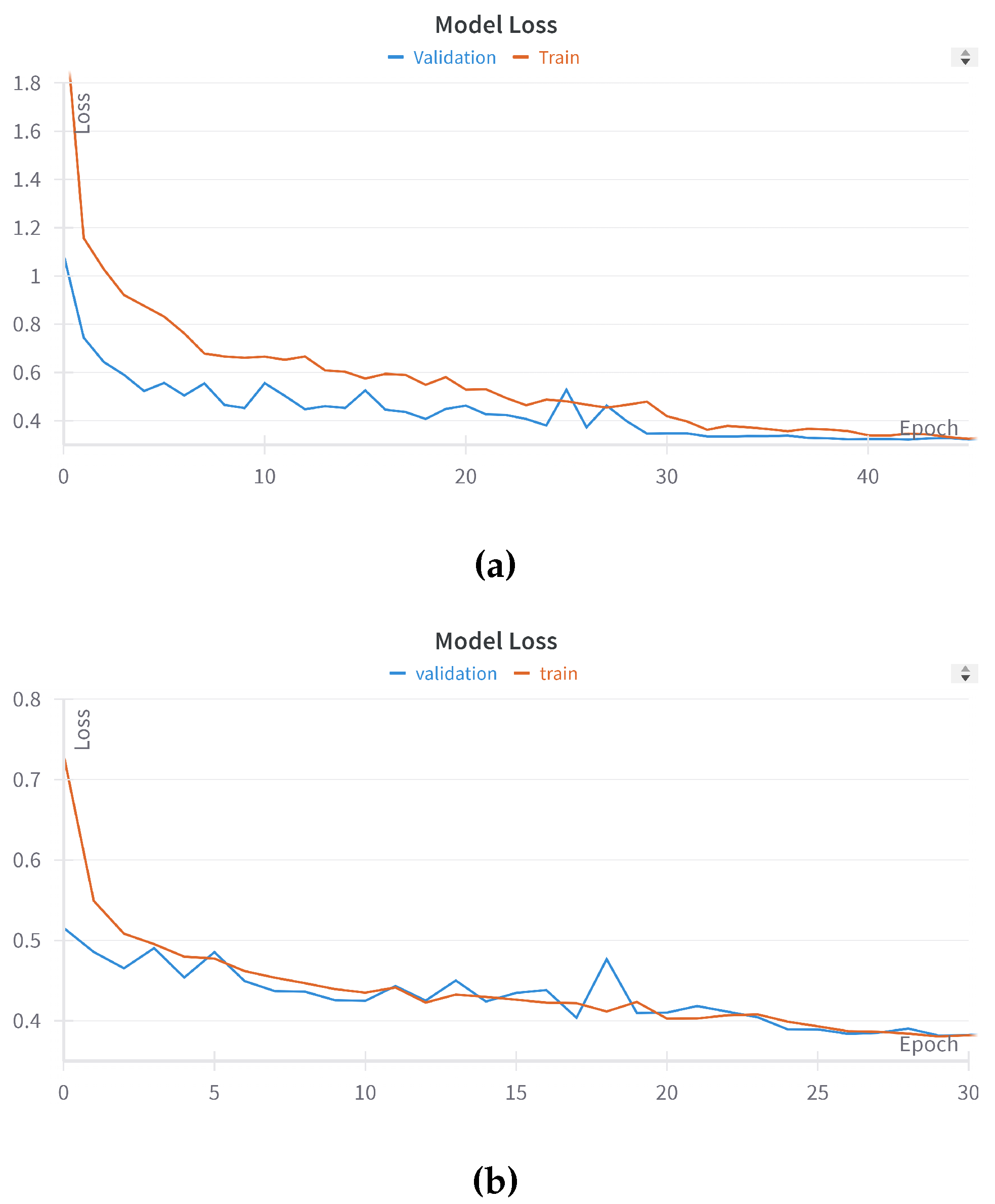
Figure 7.
Burn area segmentation result comparison across models: The left panel shows Sentinel-2 false-color images (Green, NIR, and SWIR) for the same area in Punjab. The middle panel displays ground truth data. The right panel shows the model predictions. (a) The pre-trained model (trained on Portugal) performs poorly when applied directly to Punjab, with urban areas (black circle) misclassified as burned areas, resulting in low accuracy (IoU, 0.01; Dice, 0.84). (b) After fine-tuning on Punjab data, the model shows marked improvement, accurately identifying burned areas (black arrow) while minimizing false positives leading to high accuracy (IoU, 0.73; Dice, 0.84). (c) The baseline model based on the Normalized Burn Ratio Index (NBR), overestimates burned areas, with numerous false positive results given for urban areas and healthy vegetation resulting in low accuracy (IoU, 0.03; Dice, 0.06), thereby highlighting the benefit of the model fine-tuning for region-specific burn area detection.
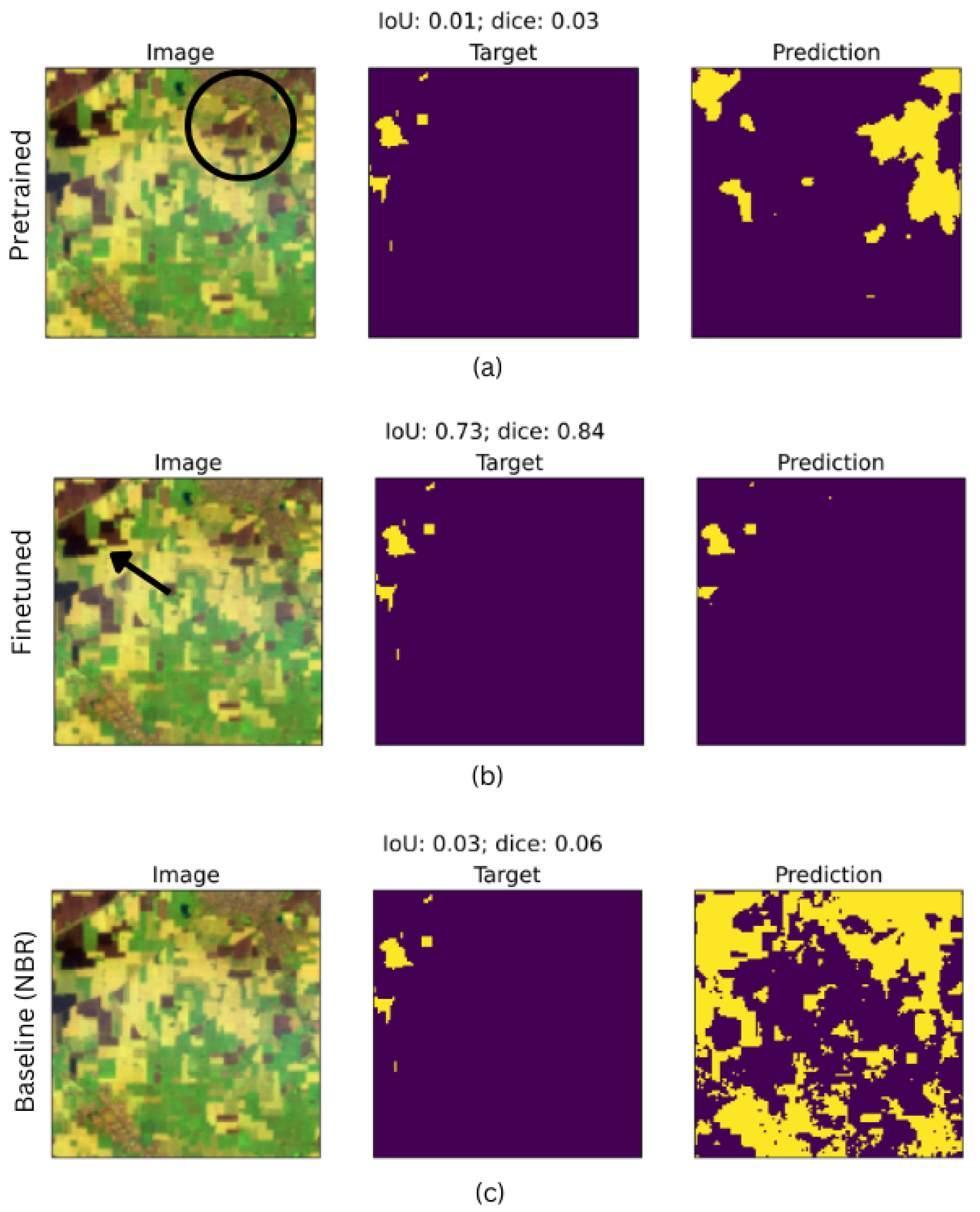
Figure 8.
Effects of architectural modification of fine-tuned models on Burn Area segmentation. The left panel shows Sentinel-2 false-color images (Green, NIR, and SWIR) for the same area in Punjab. The middle panel displays ground truth data. The right panel shows the model predictions. Figure (a) The Unmodified architecture produces a high degree of false detection over bare ground/plowed areas (refer to white circle), resulting in lower IoU (0.32) and Dice (0.49) scores. Figure (b) With the modified architecture, this false detection is reduced, leading to improved IoU (0.54) and Dice (0.70) scores. Figure (c) Unmodified architecture struggles to identify aquatic bodies resulting in false detection (white circle), whereas Figure (d) modified architecture exhibits improved detection accuracy for aquatic regions resulting in fewer false detections. Also, panel (a) shows the model improvement, with less false detection over urban areas. Panel (b) shows very precise capture of small fragmented burned crop fields, with less false detection over bare/plowed ground. Panels (c) and (d) show considerable improvement in terms of fewer false predictions over aquatic bodies.
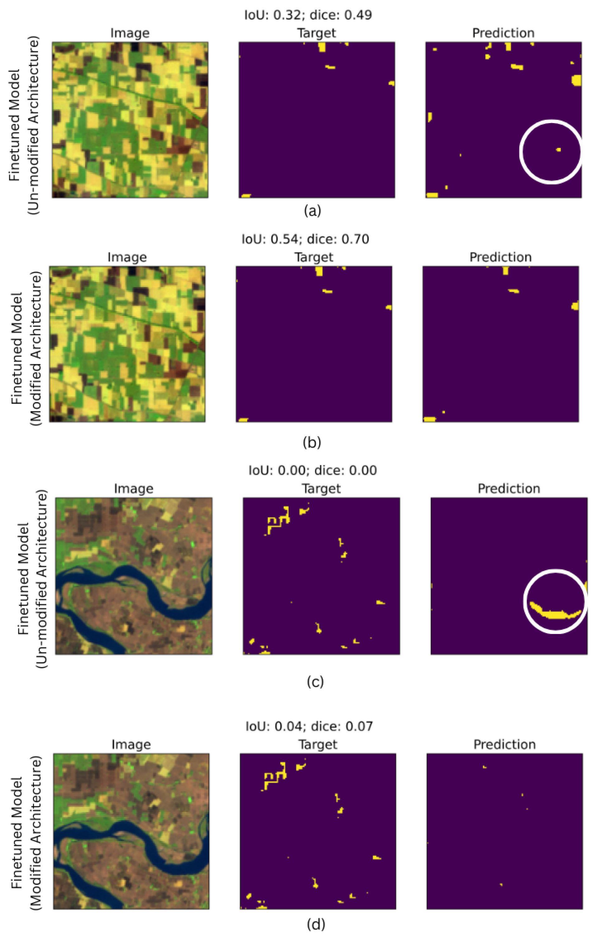
Figure 9.
Enhanced model sensitivity in capturing small burn areas after tuning with the annotated data. The left panel shows Sentinel-2 false-color images (Green, NIR, and SWIR) over Punjab. The middle panel displays hand-annotated reference data. The right panel presents model predictions. Panels (a) and (c) show predictions from the returned model: (a) shows an overestimation of burn area (black circle), (c) shows misclassification of the healthy vegetation (black circle); (b) and (d) are predictions from the fine-tuned model which reduces the overestimation of the small burn area and false detection of healthy vegetation. Fine-tuning improves the model precision compared to small burn area segmentation and reduces misclassification errors.
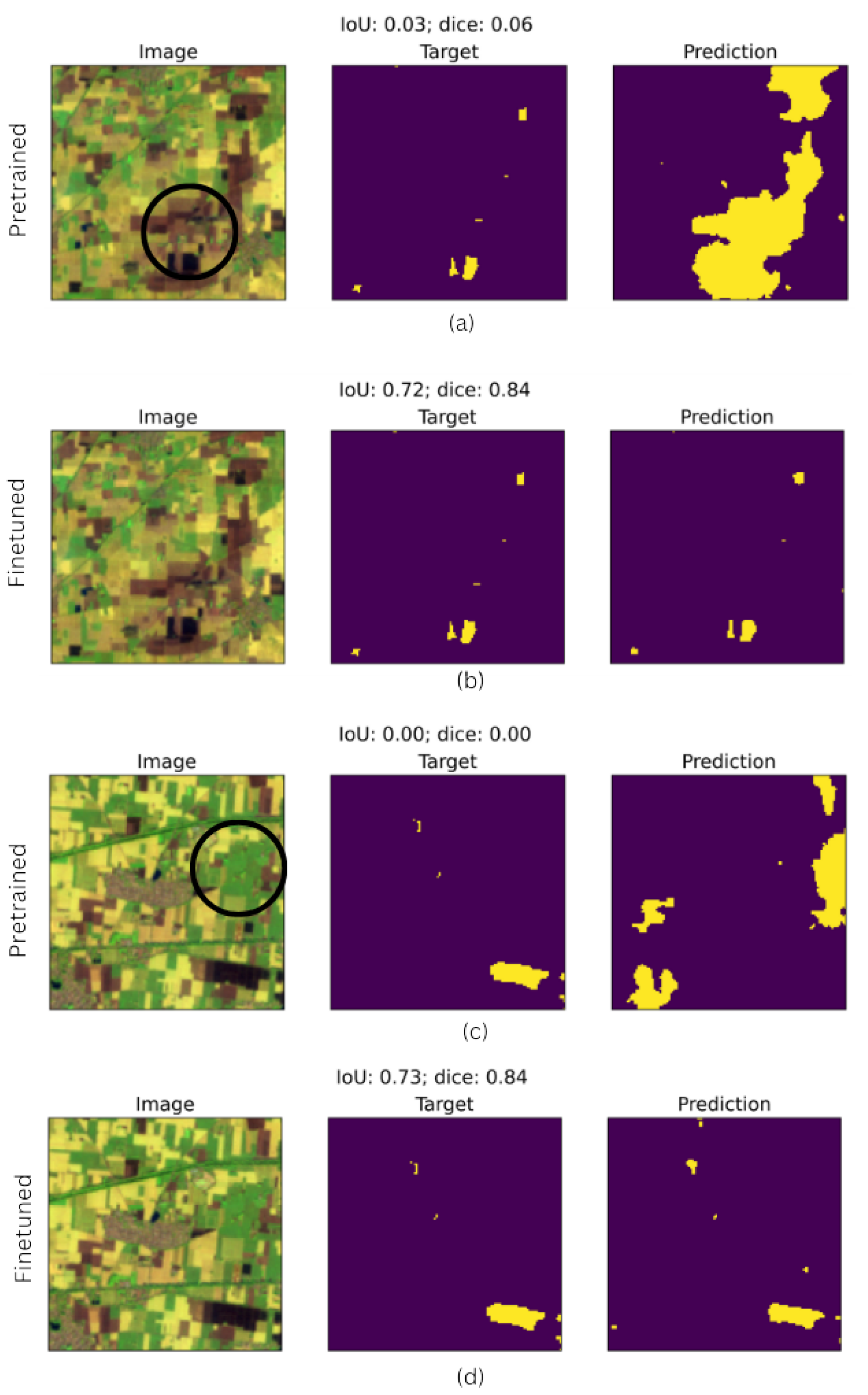
Figure 10.
Comparison of burn area prediction by the fine-tuned model and baseline model (Normalized Burn Area Index). Left panel shows Sentinel-2 false-color images (Green, NIR, and SWIR) over Punjab. Middle panel display hand-annotated reference data. Right panel present baseline model and DL model predictions. Panel (a) shows a case of false detection over healthy vegetation by baseline model whereas (b) shows burn area prediction over the same area using the DL model, burn area delineations captured more precisely and fewer false predictions over healthy vegetation. In panel (c), burn area prediction by the baseline model shows false detection over bare ground and healthy vegetation. Also, panel (d) shows burn area prediction using the DL model over the same area, with small and fragmented burn patches captured with few false predictions.
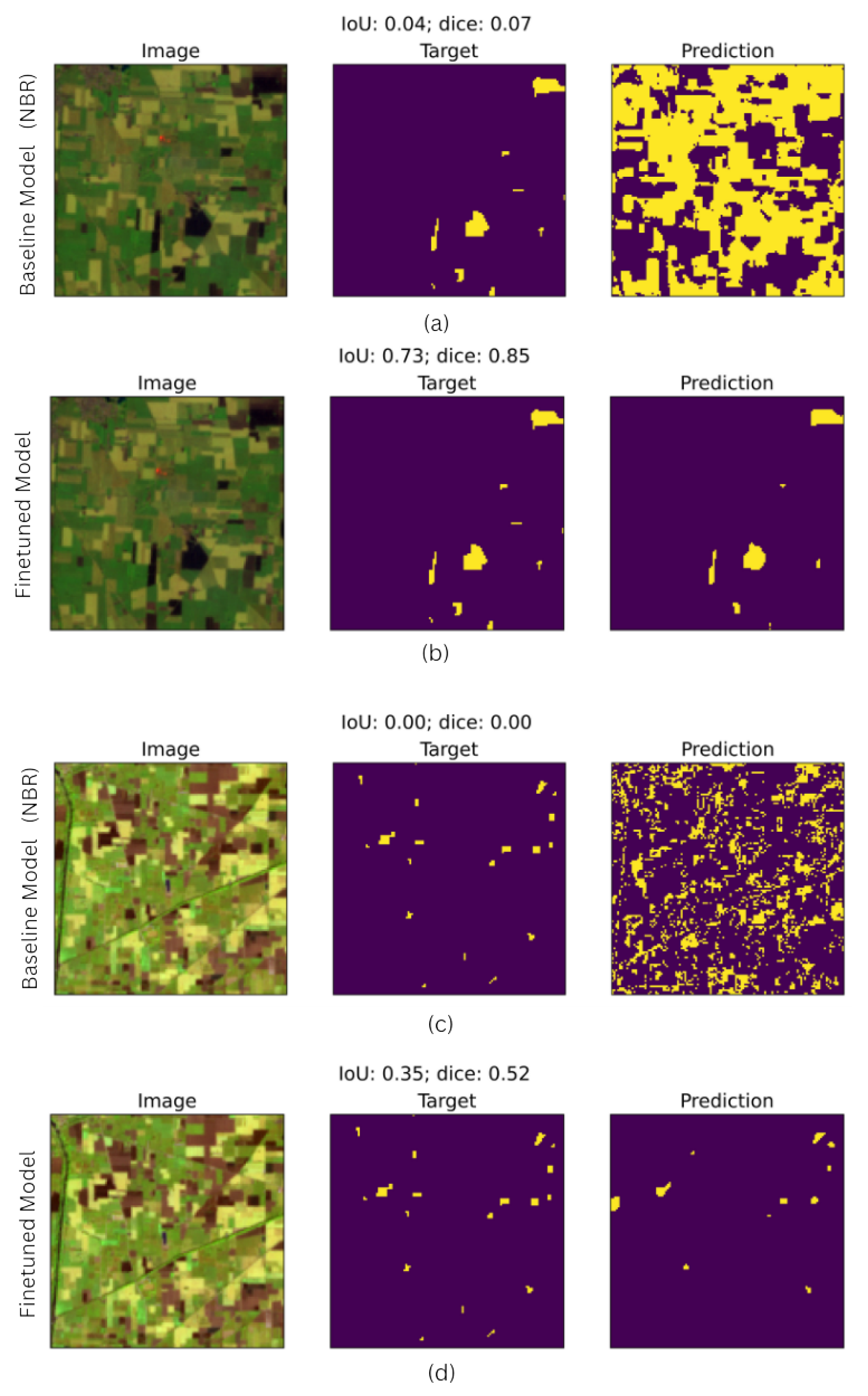
Figure 11.
On-ground validation sites in Punjab, India. Each point represents a geolocation of an image captured during November 9–11, 2020.
Figure 11.
On-ground validation sites in Punjab, India. Each point represents a geolocation of an image captured during November 9–11, 2020.
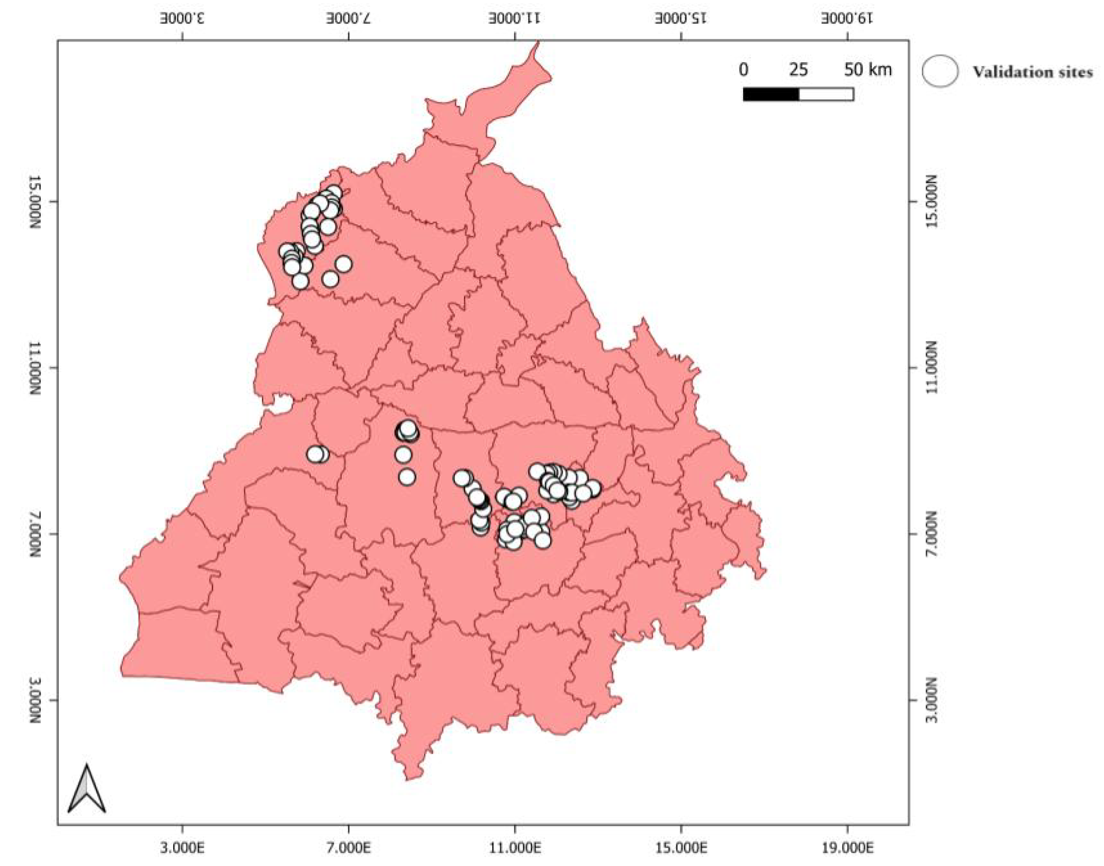
Figure 14.
Village-level monthly aggregate (composite) of burn areas during October–November using the DL model for four consecutive seasons (2020–2023).
Figure 14.
Village-level monthly aggregate (composite) of burn areas during October–November using the DL model for four consecutive seasons (2020–2023).
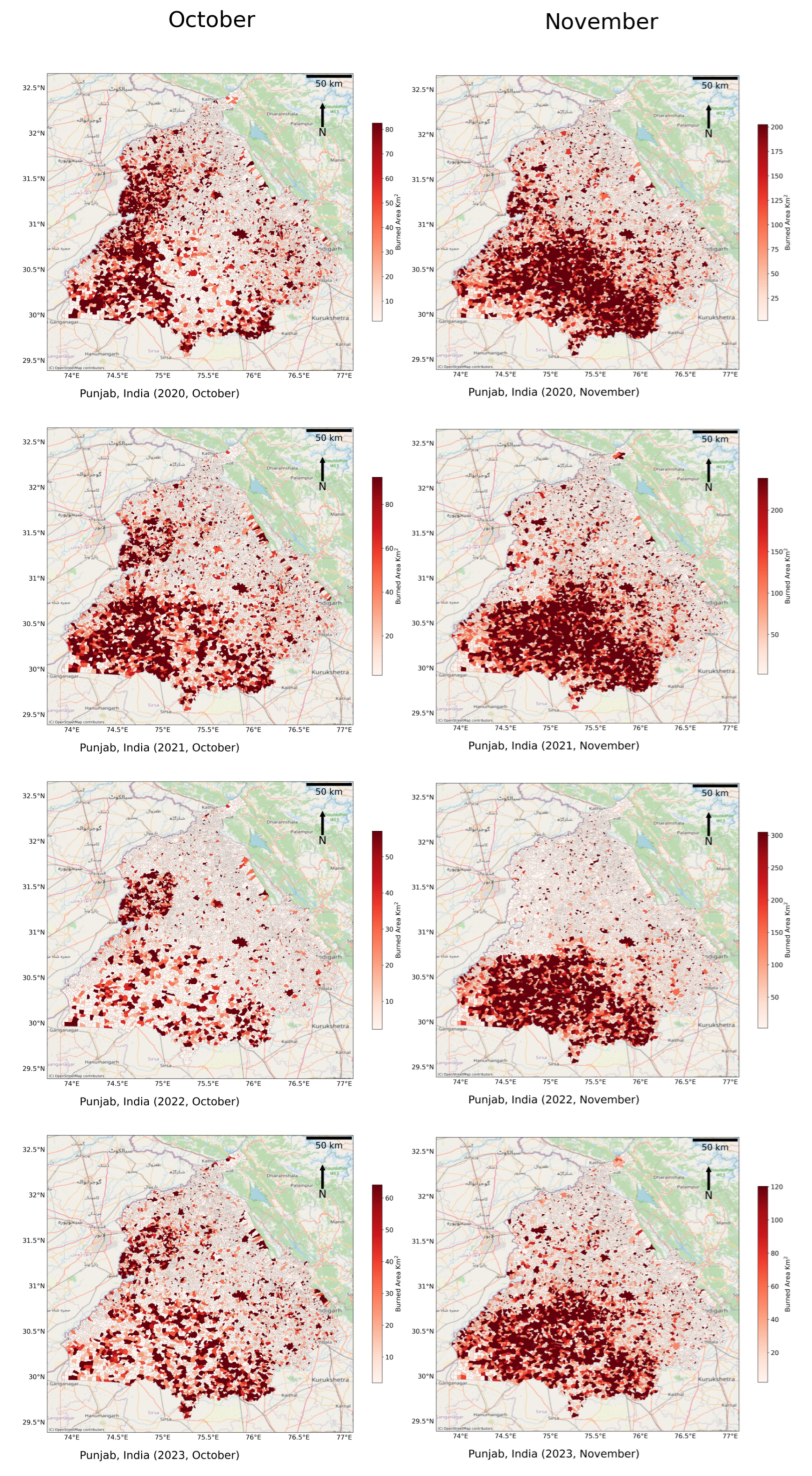
Figure 15.
Village-level monthly aggregate (composite) of burn areas during October–November using MCD64A1 for four consecutive seasons (2020–2023).
Figure 15.
Village-level monthly aggregate (composite) of burn areas during October–November using MCD64A1 for four consecutive seasons (2020–2023).
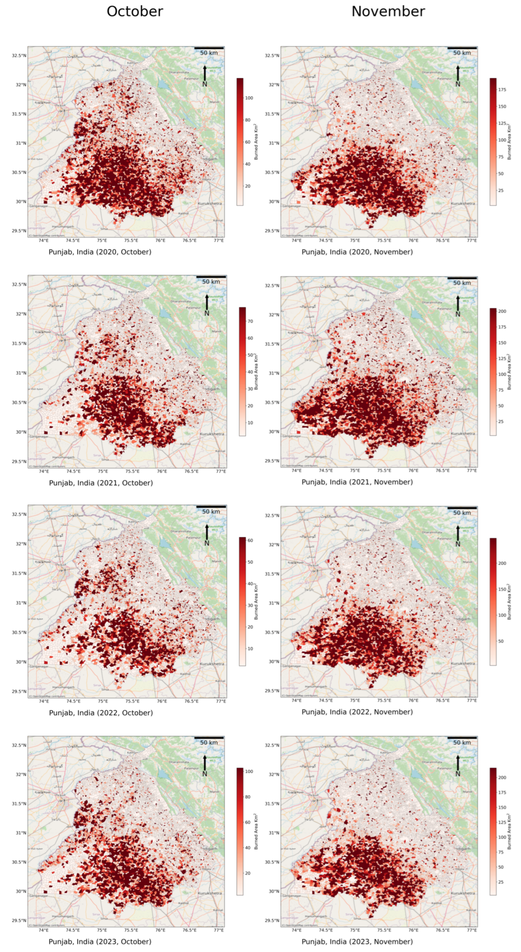
Table 2.
Performance metrics for the model trained on Portugal (Domain 1) and fine-tuned on Punjab (Domain 2)
Table 2.
Performance metrics for the model trained on Portugal (Domain 1) and fine-tuned on Punjab (Domain 2)
| Model | Domain | Type | Metric | Burned (%) | Non-burned (%) |
|---|---|---|---|---|---|
| Precision | 81.6 | 96.7 | |||
| class | Recall | 80.9 | 96.9 | ||
| F1 | 81.2 | 96.8 | |||
| DL-Model | Portugal | Accuracy (%) | 94.5 | ||
| overall | Macro-F1 (%) | 89 | |||
| IoU | 0.52 | ||||
| Dice | 0.60 | ||||
| Precision | 96 | 98.2 | |||
| class | Recall | 95.8 | 99.2 | ||
| F1 | 95.9 | 99.2 | |||
| DL-Model | Punjab | Accuracy (%) | 98.7 | ||
| overall | Macro-F1 (%) | 97.6 | |||
| IoU | 0.54 | ||||
| Dice | 0.64 | ||||
| Precision | 90.8 | 90.1 | |||
| class | Recall | 49.1 | 98.9 | ||
| F1 | 63.5 | 94.3 | |||
| Baseline (NBR) | Punjab | Accuracy (%) | 91 | ||
| overall | Macro-F1 (%) | 78 | |||
| IoU | 0.03 | ||||
| Dice | 0.05 | ||||
Disclaimer/Publisher’s Note: The statements, opinions and data contained in all publications are solely those of the individual author(s) and contributor(s) and not of MDPI and/or the editor(s). MDPI and/or the editor(s) disclaim responsibility for any injury to people or property resulting from any ideas, methods, instructions or products referred to in the content. |
© 2025 by the authors. Licensee MDPI, Basel, Switzerland. This article is an open access article distributed under the terms and conditions of the Creative Commons Attribution (CC BY) license (http://creativecommons.org/licenses/by/4.0/).
Copyright: This open access article is published under a Creative Commons CC BY 4.0 license, which permit the free download, distribution, and reuse, provided that the author and preprint are cited in any reuse.


