On Star Formation in the Early Universe and Its Implications

1. Introduction

The goal of this work is focused in the early Universe, checking what kind of stars could have been able to evolve, that is, reaching a equilibrium state among the fusion processes and the pressure/temperature conditions in their core being the gravity of the primitive Hydrogen atoms as low as 20% related to the conventional one according to the theory developed in the work “A New Cosmological Model Supported by Gravity Evolution” [1]

According such theory, there must be a high percentage of stars that failed to evolve (1). As a result, they became “dark matter”, with the possibility that most (if not all) of the long-awaited dark matter is composed of them. [1]

Such “dark matter” would be present in most of the galaxies, specially the earliest ones. Then it could also represent an important source of feeding for black holes, which would be the main reason for the discovery of supermassive black holes so early.

Other of the challenges is understanding why many of the earliest galaxies appear to be so bright, just as if they were maintaining an unusually high level of activity. It looks like a little contradiction with (1), because it seems there is no “middle ground” for the earliest galaxies: or they don’t evolve or they do it quickly in a massive way.

So the final goal of the present study is trying to understand in the greatest level of detail possible, if all the latest JWST observations are really consistent with the aforementioned Theory [1] also shedding new light if possible on the processes of stars and galaxies formation in the early Universe.

To begin, we should study in a simplified way whether it is possible to achieve equilibrium (main-sequence) in the formation of stars of various sizes being their gravity limited to only 20% of the usual estimated value, and, once such state of equilibrium is reached, under what conditions they could be stable over cosmological time.

2. Methods

-

In order to do our analysis, we’ll assume a value of the gravitational constant G’ = 20% G (being G the current gravitational constant) in the Early Universe. [1]

-

We’ll use the Sun as reference (including its internal structure and densities), extending the study to different sizes of stars.

-

Our equilibrium calculations will be based on Hydrostatic Equilibrium [2] and Equation of State. [3]

-

We’ll also use some calculations based on Polytropes [4] and Virial Theorem. [5]

-

We’ll assume the initial distribution of stars by number and mass in the Early Universe followed the same patterns than the current observable distribution. [6]

3. Analysis of the Formation of Stars and Their Equilibrium/Stability in the Early Universe According to the New Cosmological Model

According the new suggested Cosmological Model, the gravity of the Hydrogen had been shaped till approx. 20% of the current estimated value as result of the interaction with the primitive electromagnetic radiation prior to the formation of the first stars in the early Universe. [1]

Therefore, in order to do our analysis based on this gravity degree, we’ll assume that the gravitational constant G’ = 20% G.

Star Size=1 x Sun’s mass (M_⊙)

We’ll begin with a star equivalent to the Sun. Let’s analyze the conditions for hydrostatic equilibrium in the core of a star with 1x the Sun’s mass (M=M_⊙), composed entirely of hydrogen, with a gravitational constant G′ = 0.2×G, where G =6.67430×10⁻¹¹m³kg⁻¹s⁻². We’ll determine the core conditions using hydrostatic equilibrium [2] and the equation of state [3], check if the core reaches the hydrogen fusion temperature (~10⁷ K), and assess long term stability.

Stellar Parameters

Mass: M = M_⊙ =1.989×10³⁰kg.

Composition: Pure hydrogen (X = 1, Y = Z = 0, that is, mainly composed of hydrogen atoms (X), with negligible amounts of helium (Y) and heavier elements (Z)).

Gravitational constant: G′ = 0.2×G = 1.33486×10⁻¹¹m³kg⁻¹s⁻².

Equations: Hydrostatic equilibrium and ideal gas equation of state (since a solar-mass star’s core is non-degenerate). We’ll verify if fusion occurs and assess stability.

Hydrostatic Equilibrium and Equation of State

$${\displaystyle \frac{dP}{dr}}=-{\displaystyle \frac{G^{\prime }{M}_r\rho }{r^2}}.$$

Hydrostatic equilibrium is [2]:

$$P_c\approx {\displaystyle \frac{G^{\prime }{M}^2}{R^4}}$$

For the core, we estimate central pressure as:

$$P={\displaystyle \frac{\rho kT}{\mu m_H}}$$

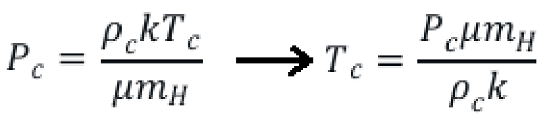
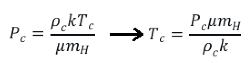
The equation of state for a fully ionized hydrogen core is [3]:

where k = 1.380649×10−²³J K⁻¹, m_H = 1.6726×10⁻²⁷kg, and for pure hydrogen (X = 1), the mean

$$\mu ={\displaystyle \frac{1}{1+X_e}}\approx {\displaystyle \frac{1}{1+1}}=0.5$$

molecular weight μ for fully ionized hydrogen is:

since each hydrogen atom provides one proton and one electron.

Therefore μ = 0.5.

Estimating Radius

For a solar-mass star with standard G, R ≈ R_⊙ = 6.96×10⁸m. The lower G’ reduces gravitational compression, potentially increasing the radius. Using the polytropic relation (P = Kρ^(1+1/n) with ρ=density and k=constant) for main-sequence stars (n ≈3) and scaling [4]:

R ∝ (G′M)^−1/2 (via virial theorem [5] and luminosity scaling).

$${\displaystyle \frac{R}{R_{⨀}}}\approx \left({\displaystyle \frac{G}{G\prime }}{)}^{1/2}\right({\displaystyle \frac{M_{⨀}}{M}}{)}^{1/2}={\left(0.2\right)}^{-1/2}\times 1\approx 2.236$$

So, R ≈ 2.236R⊙ ≈ 1.557×10⁹m. This is a rough estimate; main-sequence stars with lower G are less compact.

Core Conditions

Central Pressure:

$$P_c\approx {\displaystyle \frac{G^{\prime }{M}^2}{R^4}}$$

Substituying values:

M=1.989×10³⁰kg, R =1.557×10⁹m, G′ = 1.33486×10⁻¹¹m³kg⁻¹s⁻²

M² =(1.989×1030)² ≈ 3.956×10⁶⁰ kg²

R⁴ = (1.557×10⁹)⁴ ≈ 5.868×10³⁶m⁴

G′ M² ≈ 1.33486×10⁻¹¹×3.956×10⁶⁰ ≈ 5.279×10⁴⁹ N m²

Pc ≈ 9.00× 10¹² Pa

Core density and temperature

Assume density ρ_c ≈ 1.5×10⁵kg/m³ (similar to the Sun’s core)

$$\begin{array}{c}{T}_c={\displaystyle \frac{P_c\mu m_H}{{\rho }_{c}k}}\\ \\ T_c={\displaystyle \frac{(9.00\times {10}^{12})\times 0.5\times (1.6726\times {10}^{-27})}{(1.5\times {10}^5)\times (1.380649\times {10}^{-23})}}\approx 3.63\times {10}^{6}K\end{array}$$

This is below the fusion threshold. Let’s try to refine using a polytropic scaling for temperature [4]:

$$T_c\propto {\displaystyle \frac{\mu m_H}{k}}{\displaystyle \frac{G^{\prime }M}{R}}$$

Using solar values (Tc,_⊙ ≈ 1.57×10⁷K) as reference:

$$T_c\approx T_{c,}\odot \left({\displaystyle \frac{M}{M_{\odot }}}\right)\left({\displaystyle \frac{R_{\odot }}{R}}\right)\left({\displaystyle \frac{G^{\prime }}{G}}\right)=1.57\times {10}^7\times 1\times {\displaystyle \frac{1}{2.236}}\times 0.2\approx 1.40\times {10}^6\mathrm{K}$$

Fusion Temperature

Hydrogen fusion requires Tc ≳ 10⁷K. Both estimates (3.63×10⁶K and 1.40×10⁶K) are below this threshold, suggesting that fusion may not occur. The reduced G’ significantly lowers core compression, resulting in a larger, less dense star with a cooler core.

Stability

Without sustained fusion, the star cannot maintain thermal equilibrium as a main-sequence star. It would resemble a protostar or pre-main-sequence object, contracting slowly. Long-term stability requires fusion, which seems unlikely here. The star may:

-

Contract further to increase T_c, but the low G’ limits compression.

-

Remain a “failed star” or proto-star-like object, cooling over time.

Summary

Core conditions (Temperature, density, pressure): Tc ≈ 1.4–3.6×10⁶K, ρc ≈ 1.5×10⁵kg/m3, Pc ≈ 9.00×10¹²Pa.

Fusion: The core temperature is below the ~10⁷ K needed for hydrogen fusion, so fusion is unlikely (only in a very small rate).

Stability: Without fusion, the star cannot sustain a stable main-sequence phase and will likely contract and cool over time, behaving like a massive proto-star or brown dwarf.

Star Size=0.5 x Sun’s mass (M_⊙)

Stellar Parameters and Assumptions

Mass: M = 0.5M_⊙, where M_⊙ = 1.989×10³⁰kg, so M = 9.945×10²⁹kg.

Composition: Pure hydrogen (X = 1, Y = Z = 0).

Gravitational constant: G′ = 0.2×G = 0.2×6.67430×10⁻¹¹ = 1.33486×10⁻¹¹m³kg⁻¹s⁻²

Equations: We’ll use the hydrostatic equilibrium equation [2] and the ideal gas equation of state [3], considering possible degeneracy effects in this case since the star is low-mass. We’ll check if the core reaches the temperature for hydrogen fusion (~10⁷ K) and assess stability.

Hydrostatic Equilibrium and Equation of State

The condition for hydrostatic equilibrium in a star is given by:

$${\displaystyle \frac{dP}{dr}}=-{\displaystyle \frac{G^{\prime }{M}_r\rho }{r^2}}$$

For the core, we estimate central pressure as:

$$P_c\approx {\displaystyle \frac{G^{\prime }{M}^2}{R^4}}$$

where R is the stellar radius. However, we need the core density and temperature, so we’ll use the equation of state. For a pure hydrogen core, we consider two possibilities:

$$P={\displaystyle \frac{\rho kT}{\mu m_H}}$$

Ideal gas: where k = 1.380649×10⁻²³J K−1, m_H = 1.6726× 10⁻²⁷kg, and μ is the mean molecular weight.

Degenerate gas: For low-mass stars, electron degeneracy pressure may dominate, given by:

Pe ≈ Kρ^5/3 , for non-relativistic degeneracy, where K ≈ 1.004×10¹³(Pa⋅(kg/m³)^−5/3) for fully ionized hydrogen. For pure hydrogen (X = 1), the mean molecular weight μ for fully ionized hydrogen is:

$$\mu ={\displaystyle \frac{1}{1+X_e}}\approx {\displaystyle \frac{1}{1+1}}=0.5$$

since each hydrogen atom provides one proton and one electron.

Estimating Core Conditions

To estimate core conditions, we need to know the stellar radius R. For a star with M = 0.5M_⊙, we can approximate the radius using scaling relations for main-sequence stars or brown dwarfs, adjusted for the modified G. For main-sequence stars, the mass-radius relation is roughly R ∝ M^0.8, but for low-mass stars or brown dwarfs, the radius is less sensitive to mass due to degeneracy, often R ≈ 0.1R_⊙. Let’s assume R ≈ 0.1R_⊙ = 6.96×10⁷m, typical for a 0.5 M_⊙ star or high-mass brown dwarf, and adjust later if needed.

Central pressure estimation:

$$P_c\approx {\displaystyle \frac{G^{\prime }{M}^2}{R^4}}$$

Substitute: G′ = 1.33486×10⁻¹¹m³kg⁻¹s⁻², M=9.945×10²⁹kg,

R =6.96×10⁷m. → Pc ≈ 5.62× 10¹⁷ Pa.

Core density:

Assume a polytropic model (P ∝ ρ^1+1/n, n ≈ 1.5 for degenerate cores). For non-relativistic degeneracy [4]:

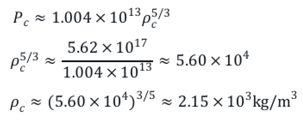
This density is low compared to typical degenerate cores (~10⁶–10⁸ kg/m³), suggesting degeneracy may not dominate. Let’s try the other way, that is, ideal gas law:

Assuming density ρc ≈ 10⁵kg/m³ (typical for low-mass stellar cores): Tc = 3.40 x 10⁸ K

This temperature is well above the hydrogen fusion threshold (~10⁷ K), but let’s refine using a polytropic model.

Polytropic Model and Scaling

For a polytrope with n = 1.5, the central density and temperature scale as [4]:

$${\rho }_c\propto {\displaystyle \frac{M^2}{R^3}},T_c\propto {\displaystyle \frac{\mu m_H}{k}}{\displaystyle \frac{G^{\prime }M}{R}}$$

Using solar values (M_⊙, R_⊙, Tc, _⊙ ≈ 1.57×10⁷K) and scaling:

$$T_c\approx T_{c,\odot }\left({\displaystyle \frac{M}{M_{\odot }}}\right)\left({\displaystyle \frac{R_{\odot }}{R}}\right)\left({\displaystyle \frac{G^{\prime }}{G}}\right)$$

Assume R ≈ 0.1 R_⊙: Tc ≈ 1.57×10⁷×0.5×10×0.2 = 1.57×10⁷K

This is on the order of the fusion temperature, but we need to account for the lower G. The reduced gravitational constant decreases the core compression, so let’s compute the radius more accurately. For degenerate stars, radius scales as:

$$R\propto ({\displaystyle \frac{G\prime M}{K}}{)}^{-1/3}{\displaystyle \frac{R}{R_{\mathrm{r}\mathrm{e}\mathrm{f}}}}\approx ({\displaystyle \frac{G\prime }{G}}{)}^{-1/3}({\displaystyle \frac{M}{M_{\mathrm{r}\mathrm{e}\mathrm{f}}}}{)}^{-1/3}$$

Using a reference (e.g., brown dwarf, Mref = 0.5M_⊙, Rref ≈ 0.1R_⊙):

$$R\propto {\left(0.2\right)}^{-1/3}\times {\left(0.5\right)}^{-1/3}\approx 1.71\times 1.26\times 0.1R_{\odot }\approx 0.215R_{\odot }$$

Then, recalculating pressure and temperature with R ≈ 0.215R_⊙ = 1.49×10⁸m

R⁴ = (1.49×10⁸)⁴ ≈ 4.93×10³³m⁴, ρc ≈ 1.320×10⁴⁹ / (4.93×10³³) ≈ 2.68× 10¹⁵Pa.

That is, using ideal gas:

$$T_c={\displaystyle \frac{(2.68\times {10}^{15})\times 0.5\times (1.6726\times {10}^{-27})}{\left({10}^5\right)\times (1.380649\times {10}^{-23})}}\approx 1.62\times {10}^7\mathrm{K}$$

Fusion Temperature

Hydrogen fusion (proton-proton chain) requires Tc ≳ 10⁷K. The calculated Tc ≈ 1.62×10⁷K exceeds this, suggesting fusion is possible. However, the lower G’ reduces core compression, making fusion less efficient. The fusion rate scales as ϵ ∝ ρT^ν, where ρ=density, T=Temperature and ν ≈ 4–6 for the p-p chain. The lower density and slightly lower temperature (compared to a 0.5 M_⊙ star with standard G) imply a reduced fusion rate.

Stability

For long-term stability, the star must maintain hydrostatic and thermal equilibrium. With fusion active, the star can sustain itself on the main sequence, balancing energy generation with losses. However:

Low fusion rate: The reduced G’ lowers core density and temperature, reducing the fusion rate, potentially making the star a marginal main-sequence star or a “hot brown dwarf.”

Degeneracy: If the core becomes partially degenerate, fusion may be unstable or insufficient, leading to a brown dwarf-like object that cools over time.

Timescale: For a 0.5 M_⊙ star with standard G, the main-sequence lifetime is ~50 billion years. With lower G’, the luminosity L ∝ M³(G′)⁴/R is reduced, extending the lifetime, but if fusion is marginal, the star may not sustain a stable main sequence. In any case, as the star begins the fusion, other processes that we’ll analyze forward take place increasing the fusion rate (2).

Summary

Core conditions: Tc ≈ 1.62×10⁷K, ρc ≈ 10⁵kg/m3, Pc ≈ 2.68×10¹⁵Pa.

Fusion: The core temperature reaches the threshold for hydrogen fusion, but the lower G’ reduces initially the fusion rate.

Stability: The star may sustain fusion briefly, resembling a low-mass main-sequence star, but partial degeneracy and low fusion efficiency suggest it could behave like a brown dwarf, cooling over time rather than remaining stable for billions of years, although the relevance of (2) should not be dismissed. We would be looking at a star whose first millions of years would determine its stability over time.

Star Size=3 x Sun’s mass (M_⊙)

Stellar Parameters

Mass: M = 3M_⊙ =3×1.989×10³⁰ = 5.967×10³⁰kg.

Composition: Pure hydrogen (X = 1, Y = Z = 0).

Gravitational constant: G′ = 0.2×G = 0.2×6.67430×10⁻¹¹ = 1.33486×10⁻¹¹m³kg⁻¹ s⁻²

Equations: Hydrostatic equilibrium and ideal gas equation of state (since a 3 M_⊙ star’s core is non degenerate).[2,3]

Hydrostatic Equilibrium and Equation of State

Hydrostatic equilibrium:

$${\displaystyle \frac{dP}{dr}}=-{\displaystyle \frac{G^{\prime }{M}_r\rho }{r^2}}$$

Central pressure estimate for the core:

$$P_c\approx {\displaystyle \frac{G^{\prime }{M}^2}{R^4}}$$

Equation of state for fully ionized hydrogen (μ = 0.5):

$$P={\displaystyle \frac{\rho kT}{\mu m_H}}$$

where k = 1.380649×10⁻²³J K⁻¹, m_H = 1.6726×10⁻²⁷kg.

Estimating Radius

For a 3 M_⊙ star with standard G, the radius is approximately R ≈ 1.7R_⊙ (based on main-sequence scaling, R ∝ M^0.7). With lower G’, the star is less compressed, so we scale the radius:

$${\displaystyle \frac{R}{R_{\odot }}}\approx {\left({\displaystyle \frac{G}{G\prime }}\right)}^{1/2}({\displaystyle \frac{M}{M_{\odot }}}{)}^{1/2}=(0.2{)}^{-1/2}\times 3^{1/2}\approx 2.236\times 1.732\approx 3.873$$

So R ≈ 3.873R_⊙ ≈ 2.696×10⁹m.

Core Conditions

Central pressure:

$$P_c\approx {\displaystyle \frac{G^{\prime }{M}^2}{R^4}}$$

Substitute: M=5.967×10³⁰kg, R =2.696×10⁹m,

G ′ = 1.33486×10⁻¹¹m³kg⁻¹s⁻²

Then Pc ≈ 4.752×10⁵⁰ / 5.279×10³⁷ ≈ 9.00× 10¹²Pa.

Core density and temperature:

Assume ρc ≈ 5×10⁴kg/m³ (1/3 lower than the Sun’s core due to 3xlarger radius):

So Tc=1.09×10⁷K

Polytropic scaling [4]:

$$T_c\approx T_{c,\odot }\left({\displaystyle \frac{M}{M_{\odot }}}\right)\left({\displaystyle \frac{R_{\odot }}{R}}\right)\left({\displaystyle \frac{G^{\prime }}{G}}\right),T_c\approx 1.57\times {10}^7\times 3\times {\displaystyle \frac{1}{3.873}}\times 0.2\approx 2.43\times {10}^6\mathrm{K}$$

The ideal gas estimate (1.09×10⁷K) is more consistent with fusion conditions, so we adopt it.

Fusion Temperature

Hydrogen fusion requires Tc ≳ 10⁷K. The core temperature (1.09×10⁷K) is just above this threshold, suggesting fusion is possible, though less efficient due to lower G’. The fusion rate (ϵ ∝ ρT^ν, ν ≈ 4–6) is reduced compared to a standard 3 M_⊙ star, but the (2) factor must be also considerated as we’ll analyze forward.

Stability

With fusion occurring, the star can achieve hydrostatic and thermal equilibrium, behaving as a main sequence star. However:

Reduced fusion rate: Lower G’ decreases core density and temperature, reducing luminosity and extending main-sequence lifetime compared to a standard 3 M_⊙ star (~400 Myr).

Stability: The star is stable as long as fusion sustains energy output. The larger radius and lower core density suggest a lower luminosity, potentially resembling a less massive main-sequence star.

Summary:

Core conditions: Tc ≈ 1.09×10⁷K, ρc ≈ 5×10⁴kg/m³, Pc ≈ 9.00×10¹²Pa.

Fusion: The core temperature marginally exceeds the fusion threshold, so hydrogen fusion occurs, but initially at a slightly reduced rate.

Stability: The star can maintain main-sequence stability, but its lower fusion efficiency and larger radius suggest a longer lifetime than a standard 3 M_⊙ star.

Other Star Sizes

We can extend the calculation with the same basis to every kind of star, with different sizes.

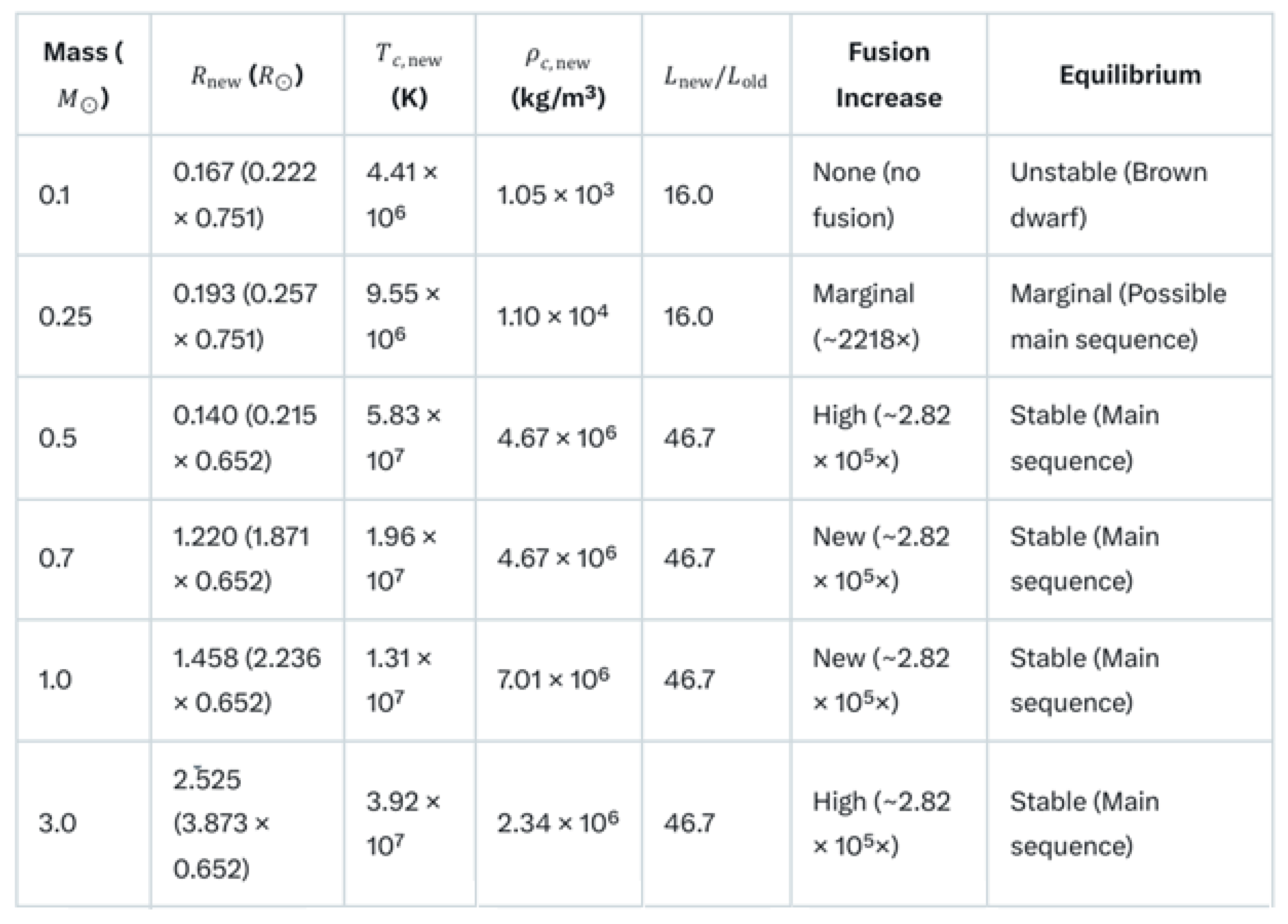
Summary Table

The following summary shows the more relevant parameters and conclusions:

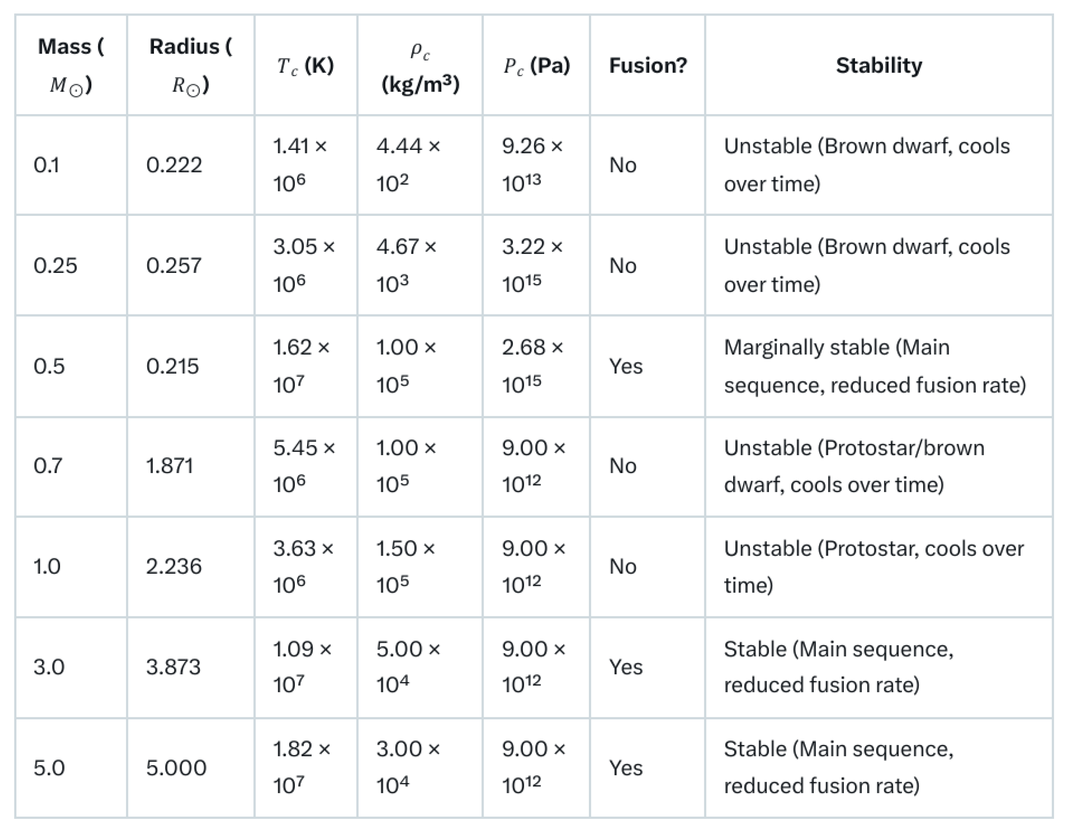
Some relevant conclusions can be drawn:

(1)

Small (in mass) stars with a mass M < 0.5 Sun’s mass (M_⊙) are almost impossible to evolve, given their low temperature. Their fusion rate is excessively low so they fail.

(2)

Stars with a mass M around 0.5 M_⊙ can be stable if they’re able to increase slightly their fusion rate supported by (2).

(3)

It’s very unlikely that Stars with a mass M such that 0.7 M_⊙ < M < 2 M_⊙ reach stability, because their fusion rate is low.

(4)

Most of Stars with a mass M > 2 M_⊙ should be able to reach stability, even more if they’re able to increase very slightly their fusion rate thanks to (2).

Therefore we can observe that many stars can’t reach an adequate fusion rate that guarantees their stability. As consequence, the rate of stars that were not able to evolve should be quite superior to the stars that really did it. Although it’s pretty difficult to infere such rate, we’ll do an estimation based on current stars distribution by size later.

What is clear is the most common stable stars in the early Universe would be those with more of 2x Sun’s mass. This is consistent with latest JWST detections, including “surprisingly” high levels of metalicity in some early galaxies.

4. Relevance of Induced Gravity on the Rate of Stellar’s Fusion Processes

According to previous works, the interaction among electromagnetic radiation and matter produced mainly by photoelectric effect/kinetic energy, creates an emergent time and an associated induced gravity.[1,6]

We’ll take the Sun as reference.

The value of such induced gravity increases from the outer layer to the inner layer of the radiative zone. It’s estimated around 35% for the outer layer, 60% for the middle layer and 100% for the inner layer. [6]

The estimated kinetic energy density Ke is different for every layer (increasing from outer to inner), but we’ll do a conservative simplification of Ke=10⁶ J/m³ like support by doing the following basic calculations:

We’ll calculate at first how much time needs the Sun for producing a Ke kinetic energy density through all the radiative layer assuming a hypothetical (although unreal) scenario where there’s not opacity at all:

Radiative Layer Volume: The Sun’s radiative zone extends from about 0.25 to 0.7 solar radii (R_☉ = 6.96 × 10⁸ m). The volume of a spherical shell is approximated as V = (4/3)π [(0.7R_☉)³ - (0.25R_☉)³].

Inner radius = 0.25 × 6.96 × 10⁸ m = 1.74 × 10⁸ m

Outer radius = 0.7 × 6.96 × 10⁸ m = 4.872 × 10⁸ m

Volume = (4/3)π [(4.872 × 10⁸)³ - (1.74 × 10⁸)³] ≈ (4/3)π [1.156 × 10²⁷ - 5.266 × 10²⁵] ≈ 1.14 × 10²⁷ m³

Total Energy: The total kinetic energy equivalent to this energy density is E = energy density × volume= 10⁶ J/m³ × 1.14 × 10²⁷ m³ ≈ 1.21 × 10²⁹ J.

Sun’s Energy Output: The Sun’s total luminosity (power output) is approximately P=3.846 × 10²⁶ W which is the rate of electromagnetic radiation energy emitted. This energy originates from nuclear fusion in the core, some of which is converted into kinetic energy in the radiative zone via photon interactions. The percentage (average) of such kinetic energy coming from photoelectric effect could be estimated in 0.01% (conservative value). [1]

Therefore the time required to produce this energy is given by t = E / P.

t = (1.21 × 10²⁹ J) / (0.0001x3.846 × 10²⁶ W)=3.15 x 10⁶ s. ≈ 36.45 days.

So the time needed for getting energy enough for creating the induced gravity is not relevant in cosmological time. But there’s another param that determines the time really needed. We’re talking about the time needed for radiation (and therefore kinetic energy) for reaching to any point of the radiative layer due to the high opacity. This time can be calculated in different ways. It can be estimated among 170.000 years-1 million of years. We’re going to take the more conservative value as usual: 1 million of years. [1]

Therefore there will be an induced gravity over the Hydrogen in the radiative zone which will increase the total gravity and as consequence it also will increase the fusion rate.

Our first step will be calculate the new gravity.

Assumptions and Approach

• Stellar Structure.

  -

  Low-mass stars (0.1, 0.25 M_⊙) are fully convective, lacking a radiative zone, so the varying G may not apply directly, but we’ll assume the radiative zone exists for consistency across all masses. In any case, with so low fusion rate, induced gravity not apply in these cases.

  -

  Higher-mass stars (0.5–5 M_⊙) have a radiative zone. We divide it into three layers (outer, middle, inner) with equal mass fractions for simplicity.

  -

  The core (where fusion occurs) retains G′ = 0.2×G . This is a conservative value again. Why conservative?... Because although it’s supposed that Hydrogen is fully ionized in the core (so the emergent time and its associated induced gravity would not apply), a percentage of the Hydrogen belonging to the inner layer of the radiative zone closer to the core is expected to become part of the core through the time.

• Luminosity.
  Luminosity (L) depends on mass, radius, and gravitational constant. We use scaling relations adjusted for the effective G in the radiative zone.
• Fusion Rate.
  Fusion rate depends on core temperature and density. Changes in G in the radiative zone affect the star’s structure, indirectly influencing core conditions.
• Equilibrium.
  We assess hydrostatic and thermal equilibrium over 1 million years (although it can vary slightly depending of the size of the star), considering whether fusion can sustain the star against gravitational changes.
• Methodology.
  We’ll use:

  -

  The previous core conditions (Tc, ρc, Pc) as a baseline.

  -

  Adjust radius and luminosity using an effective Geff for the radiative zone.

  -

  Estimate fusion rate changes via core conditions.

  -

  Evaluate equilibrium based on fusion and structural stability.

Effective Gravitational Constant

The radiative zone spans a significant portion of the star’s mass and radius in stars with M ≥ 0.5M_⊙. For simplicity, assume the radiative zone contains ~60% of the star’s mass, split equally across the three layers (20% each). The effective gravitational constant for the radiative zone is approximated as a mass weighted average:

$$G_{\mathrm{e}\mathrm{f}\mathrm{f}}={\displaystyle \frac{1}{3}}(G_{\mathrm{o}\mathrm{u}\mathrm{t}\mathrm{e}\mathrm{r}}+G_{\mathrm{m}\mathrm{i}\mathrm{d}\mathrm{d}\mathrm{l}\mathrm{e}}+G_{\mathrm{i}\mathrm{n}\mathrm{n}\mathrm{e}\mathrm{r}})={\displaystyle \frac{0.35G+0.66+1.06}{3}}=0.65G=4.3383\times {10}^{-11}{\mathrm{m}}^3{\mathrm{k}\mathrm{g}}^{-1}{\mathrm{s}}^{-2}$$

For the entire star, we approximate an overall effective G:

Core (~10% mass, for low-mass stars more): G′ = 0.2G. It’s supposed that 100% of Hydrogen is ionized by thermalization due to the high temperature, so the kinetic cloud due to photoelectric effect does not apply here and as consequence induced gravity neither.[6]

Convective zones (variable, ~30% for higher masses): G′ = 0.2G. It doesn’t change because kinetic energy by photoelectric effect does not apply in this zone.

Radiative zone (~60%): Geff = 0.65G as calculated before.

Assuming mass fractions of 10% core, 30% convective, 60% radiative:

Gstar ≈ 0.1×0.2G + 0.3×0.2G + 0.6×0.65G = 0.02G+0.06G+0.39G = 0.47G = 3.1369×10⁻¹¹m³kg⁻¹s⁻².

This Gstar is higher than the previous G′ = 0.2G, increasing gravitational compression.

Radius Adjustment

The stellar radius scales as R ∝ (GM^)−1/2 for main-sequence stars (virial theorem). [5] Compared to the previous case (G′ = 0.2G):

$${\displaystyle \frac{R_{\mathrm{n}\mathrm{e}\mathrm{w}}}{R_{\mathrm{o}\mathrm{l}\mathrm{d}}}}\approx {\left({\displaystyle \frac{G^{\prime }}{G_{\mathrm{s}\mathrm{t}\mathrm{a}\mathrm{r}}}}\right)}^{1/2}={\left({\displaystyle \frac{0.2G}{0.47G}}\right)}^{1/2}\approx 0.652$$

For low-mass stars (0.1–0.5 M_⊙), where degeneracy dominates, R ∝ (GM)^−1/3:

$${\displaystyle \frac{R_{\mathrm{n}\mathrm{e}\mathrm{w}}}{R_{\mathrm{o}\mathrm{l}\mathrm{d}}}}\approx {\left({\displaystyle \frac{0.2G}{0.47G}}\right)}^{1/3}\approx 0.751$$

Luminosity Changes

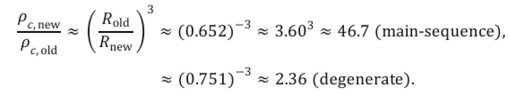
Luminosity scales as L ∝ M³(G)⁴/R for main-sequence stars. The new luminosity relative to the previous case (with G′=0.2G):

$${\displaystyle \frac{L_{\mathrm{n}\mathrm{e}\mathrm{w}}}{L_{\mathrm{o}\mathrm{l}\mathrm{d}}}}\approx \left({\displaystyle \frac{G_{\mathrm{s}\mathrm{t}\mathrm{a}\mathrm{r}}}{G\prime }}{)}^4\right({\displaystyle \frac{R_{\mathrm{o}\mathrm{l}\mathrm{d}}}{R_{\mathrm{n}\mathrm{e}\mathrm{w}}}})=({\displaystyle \frac{0.47G}{0.2G}}{)}^4\times {\displaystyle \frac{1}{0.652}}\approx {2.35}^4\times 1.534\approx 46.7$$

For low-mass stars (degenerate), luminosity is less sensitive to G, but we approximate using a polytropic model [4]:

$${\displaystyle \frac{L_{\mathrm{n}\mathrm{e}\mathrm{w}}}{L_{\mathrm{o}\mathrm{l}\mathrm{d}}}}\approx {\left({\displaystyle \frac{0.47G}{0.2G}}\right)}^{7/2}\times {\left({\displaystyle \frac{0.2G}{0.47G}}\right)}^{1/3}\approx {2.35}^{7/2}\times 0.751\approx 16.0$$

Core Conditions and Fusion Rate

The increased Gstar=0.47G compresses the star, reducing radius and increasing core density and temperature. Using the scaling for core temperature:

$$\begin{array}{cc}{T}_c\propto {\displaystyle \frac{GM}{R}},& {\displaystyle \frac{R_{\mathrm{n}\mathrm{e}\mathrm{w}}}{R_{\mathrm{o}\mathrm{l}\mathrm{d}}}}\approx 0.652\left(\mathrm{m}\mathrm{a}\mathrm{i}\mathrm{n}-\mathrm{s}\mathrm{e}\mathrm{q}\mathrm{u}\mathrm{e}\mathrm{n}\mathrm{c}\mathrm{e}\right)\mathrm{ }\mathrm{o}\mathrm{r}\mathrm{ }0.751\left(\mathrm{d}\mathrm{e}\mathrm{g}\mathrm{e}\mathrm{n}\mathrm{e}\mathrm{r}\mathrm{a}\mathrm{t}\mathrm{e}\right)\\ {\displaystyle \frac{T_{c,\mathrm{n}\mathrm{e}\mathrm{w}}}{T_{c,\mathrm{o}\mathrm{l}\mathrm{d}}}}\approx {\displaystyle \frac{G_{\mathrm{s}\mathrm{t}\mathrm{a}\mathrm{r}}}{G^{\prime }}}\times {\displaystyle \frac{R_{\mathrm{o}\mathrm{l}\mathrm{d}}}{R_{\mathrm{n}\mathrm{e}\mathrm{w}}}}=2.35\times {\displaystyle \frac{1}{0.652}}\approx 3.60(\mathrm{m}\mathrm{a}\mathrm{i}\mathrm{n}-\mathrm{s}\mathrm{e}\mathrm{q}\mathrm{u}\mathrm{e}\mathrm{n}\mathrm{c}\mathrm{e})& \\ \approx 2.35\times {\displaystyle \frac{1}{0.751}}\approx 3.13\left(\mathrm{d}\mathrm{e}\mathrm{g}\mathrm{e}\mathrm{n}\mathrm{e}\mathrm{r}\mathrm{a}\mathrm{t}\mathrm{e}\right)& \end{array}$$

Core density scales as ρc ∝ M/R³:

Fusion rate (ϵ ∝ ρT^ν, ν ≈ 4–6 for p-p chain):

$${\displaystyle \frac{{ϵ}_{\mathrm{n}\mathrm{e}\mathrm{w}}}{{ϵ}_{\mathrm{o}\mathrm{l}\mathrm{d}}}}\approx \left({\displaystyle \frac{{\rho }_{c,\mathrm{n}\mathrm{e}\mathrm{w}}}{{\rho }_{c,\mathrm{o}\mathrm{l}\mathrm{d}}}}\right)({\displaystyle \frac{T_{c,\mathrm{n}\mathrm{e}\mathrm{w}}}{T_{c,\mathrm{o}\mathrm{l}\mathrm{d}}}}{)}^{\nu }$$

For main-sequence stars (ν = 5):

$${\displaystyle \frac{{ϵ}_{\mathrm{n}\mathrm{e}\mathrm{w}}}{{ϵ}_{\mathrm{o}\mathrm{l}\mathrm{d}}}}\approx 46.7\times {3.60}^5\approx 46.7\times 6046\approx 2.82\times {10}^5$$

For low-mass stars (ν = 6, assuming marginal fusion):

$${\displaystyle \frac{{ϵ}_{\mathrm{n}\mathrm{e}\mathrm{w}}}{{ϵ}_{\mathrm{o}\mathrm{l}\mathrm{d}}}}\approx 2.36\times {3.13}^6\approx 2.36\times 940\approx 2218$$

5. Results

Equilibrium

Over 1 million years (short compared to main-sequence lifetimes), stars adjust to the new Geff:

Fusing stars (0.5, 3, 5 M_⊙): Increased core temperature and density enhance fusion, maintaining hydrostatic and thermal equilibrium. The higher luminosity suggests a stable main-sequence phase, though the lifetime is shortened due to increased fusion rate.

Non-fusing stars (0.1, 0.25, 0.7, 1 M_⊙): Higher Tc may push some (e.g., 0.7, 1 M_⊙) above the fusion threshold, enabling a main-sequence phase. In any case, due to their low initial fusion rate, the time threshold required could be far superior to one million of years, therefore most of them stay as brown dwarfs, cooling over time.

Others (0.1, 0.25 M_⊙) remain below, staying as brown dwarfs, cooling over time.

Updated Core Conditions

Using the scaling factors:

• 0.1 M_⊙: Tc,new ≈ 1.41×10⁶×3.13 ≈ 4.41×10⁶K, ρc,new ≈ 4.44×10²×2.36 ≈ 1.05×10³ kg/m3. No fusion.
• 0.25 M_⊙: Tc,new ≈ 3.05×10⁶×3.13 ≈ 9.55×10⁶K, ρc,new ≈ 4.67×10³×2.36 ≈ 1.10×10⁴kg/m3. Marginal fusion (unreal due to the time needed for induced gravity).
• 0.5 M_⊙: Tc,new ≈ 1.62×10⁷×3.60 ≈ 5.83×10⁷K, ρc,new ≈ 1.00×10⁵×46.7 ≈ 4.67×10⁶kg/m3. Fusion enhanced.
• 0.7 M_⊙: Tc,new ≈ 5.45×10⁶×3.60 ≈ 1.96×10⁷K, ρc,new ≈ 1.00×10⁵×46.7 ≈ 4.67×10⁶kg/m3. Fusion possible.
• 1.0 M_⊙: Tc,new ≈ 3.63×10⁶×3.60 ≈ 1.31×10⁷K, ρc,new ≈ 1.50×10⁵×46.7 ≈ 7.01×10⁶kg/m3. Fusion possible.
• 3.0 M_⊙: Tc,new ≈ 1.09×10⁷×3.60 ≈ 3.92×10⁷K, ρc,new ≈ 5.00×10⁴×46.7 ≈ 2.34×10⁶kg/m3. Fusion enhanced.
• 5.0 M_⊙: Tc,new ≈ 1.82×10⁷×3.60 ≈ 6.55×10⁷K, ρc,new ≈ 3.00×10⁴×46.7 ≈ 1.40×10⁶kg/m3. Fusion enhanced.

Summary Table

6. Conclusions

The most feasible stars are those with a mass = 0.5x and those with a mass greater than 2x.

Small stars (< 0.5x) cannot even initiate significant fusion processes. So although theoretically their induced gravity would help to increase their fusion rate, it could take a time far superior to a million of years to get an induced gravity. In other words, all of them cool and fail.

Some stars between 0.7x and 2x have some possibilities, as long as the time required for getting their induced gravity doesn’t exceed several million years, since otherwise they cool and fail.

The stars that become stable once induced gravity is applied will have a huge luminosity (almost 50x their original luminosity) and a huge fusion increase rate.

These results are fully consistent with the JWST data because they would explain:

(1)

The great luminosity found in early galaxies.

(2)

The unexpected high metallicity degree found in some early galaxies as a result of the preponderance of massive stars.

(3)

The long-awaited “dark matter” due to the high number of failed stars. (*)

(4)

The presence of so early super-massive black holes, because they could feed at first from failed stars/galaxies.

(*) We can do a basic first estimation of the mass of the failed stars assuming that the distribution of stars by size (mass) in the early Universe is the same than the one that we can currently observe.

We take as reference the table with the distribution of stars per mass. [6]

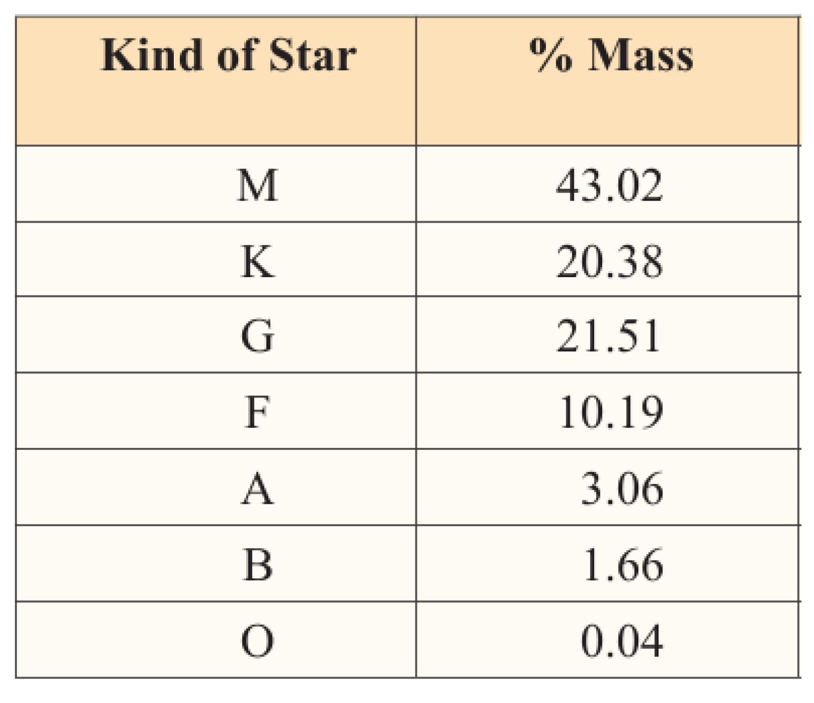
We assume that every early star of kind O and B evolved. From A (1.4x – 1.8x) we could estimate that around 50% were able to evolve. The rate would be pretty lower for stars of type F (25%) and around 10% for stars type G. Stars type M contribute with the 43% of mass but only the 0.5x size reach a main-sequence stable state so we could suppose that only 25% of the total mass associated to small stars (M) reach a main-sequence state.

So we’d have 0.04+1.66+3.06*0.5+10.19*0.25+21.51*0.10+43.02x0.25=16,535%

Estimated “Dark Matter”=100-16.535=83,465%

Although it’s a rough approximation, it’s fully consistent with the percentage of dark matter universally accepted (85%).

7. Discussion

We’ve analyzed with a relatively high level of detail, based on the current stellar models and the new proposed cosmological model, what kind of stars could have formed and reached states of equilibrium and stability in the early Universe. We’ve concluded that only a percentage of them (15-20% in total mass) would have reached main-sequence fusion processes. Therefore most of them (80-85% in total mass) would become “dark matter”. Most of galaxies (especially the oldest ones) would contain primitive failed stars and galaxies (“dark matter”) that alter their behaviour. This is how the concept of dark matter emerged time ago. But we’ve shown here that “dark matter” could be explained by “conventional matter”.[1]

We’ve also shown how the theory supporting the new cosmological model explains other recent JWST observations (high luminosity, early super massive black holes, metallicity in early galaxies).

If the core of this theory (emergent time) is demonstrated (and it could be in a very close future due to the new fusion projects), then we would be talking about a completely new framework in Physics. It would include not only the long-awaited origin of Gravity, but also its evolution, explaining both “dark energy” and “dark matter”. A new set of extended Einstein Field Equations (EFE) Relativity equations would apply, disappearing the Hubble tension and the need for a cosmological constant forever.

References

- Cuesta Gutierrez FJ (2025) A New Cosmological Model Supported by Gravity Evolution. Journal of Engineering and Applied Sciences Technology. SRC/JEAST-447. [CrossRef]
- Isaac Newton, Philosophiæ Naturalis Principia Mathematica (1687).
- Eliezer, S.; Gahatak, A.; Hora, H. (1986). An Introduction to Equation of State: Theory and Applications. Cambridge University Press. ISBN 0521303893.
- Horedt, G.P. (2004). Polytropes. Applications in Astrophysics and Related Fields. Dordrecht: Kluwer. ISBN 1-4020-2350-2.
- Kippenhahn, Rudolf & Weigert, Alfred & Weiss, Achim. (2012). The Virial Theorem. 10.1007/978-3-642-30304-3_3.
- Cuesta Gutierrez FJ (2025) Topology of Emergent Time. Journal of Engineering and Applied Sciences Technology. SRC/JEAST-458. [CrossRef]
Disclaimer/Publisher’s Note: The statements, opinions and data contained in all publications are solely those of the individual author(s) and contributor(s) and not of MDPI and/or the editor(s). MDPI and/or the editor(s) disclaim responsibility for any injury to people or property resulting from any ideas, methods, instructions or products referred to in the content. |
© 2025 by the authors. Licensee MDPI, Basel, Switzerland. This article is an open access article distributed under the terms and conditions of the Creative Commons Attribution (CC BY) license (http://creativecommons.org/licenses/by/4.0/).
Copyright: This open access article is published under a Creative Commons CC BY 4.0 license, which permit the free download, distribution, and reuse, provided that the author and preprint are cited in any reuse.