Submitted:
12 August 2025
Posted:
13 August 2025
You are already at the latest version
Abstract
This article presents a novel algebraic approach—Algebraic Modeling of Evolution of System (ALMODES)—for analyzing and simulating the dynamic evolution of social systems, with a particular focus on sustainable development strategies. The study addresses the need for effective, accessible modeling tools to capture the temporal complexity of social systems, a challenge frequently encountered using traditional system dynamics methods reliant on continuous time and differential equations. ALMODES employs discrete time steps and matrix algebra closely tied to directed graph representations, thus offering intuitive model structuring, reduced data requirements, and transparent simulation of system states over time. The method’s applicability is demonstrated through two case studies: (1) a model of urban public health dynamics, illustrating the interplay between migration, modernization, sanitation, and disease under various scenarios; and (2) a strategic model for a high-tech service company, where the integration of the Balanced Scorecard framework with ALMODES captures customer and employment fluctuations and supports evaluation of interventions such as hiring and productivity enhancements. Simulation results highlight how strategic parameter adjustments can stabilize system performance, reduce undesired fluctuations, and support more sustainable outcomes. The findings suggest that ALMODES is a versatile, computationally efficient tool for supporting both research and management of complex social systems in the context of sustainable development.
Keywords:
Algebraic Modeling of Evolution of System (ALMODES)
; decision support
; simulation model
; sustainable development
; system dynamics
1. Introduction
1.1. Systemic Approach in Social Sciences
The systemic approach in social sciences has yielded diverse solutions, often characterized by a static perspective. These solutions involve achieving a stable state of the system through a series of operations, potentially infinite in number. Implicitly, these methods assume that internal processes within the system evolve rapidly compared to the observation period. The primary interest of the researcher lies in the final, typically stable state, which serves as a valuable source of information about the system under investigation.
Two pioneering research projects at Battelle were among the first attempts to model complex social systems. These efforts led to the development of two graphical representation methods for problem analysis: Interpretive Structural Modeling (ISM) [1,2,3] and the Decision Making Trial and Evaluation Laboratory (DEMATEL) [4,5,6,7]. Both methods are still popular today (e.g., [3,8,9]).
Both ISM and DEMATEL utilize digraphs and matrices to represent relationships. ISM employs Boolean matrices to identify relationships and system structure [10]. In contrast, DEMATEL measures direct impacts on a ratio scale, typically limited to a few points (e.g., 1, 2, 3, 4). Through appropriate scaling, DEMATEL can assess total interactions within the digraph, considering paths of any length. The elements of the output matrix can be combined to compare the significance of system components and their relative positions as ’causal’ or ’affected.’
The Weighted Influence Non-linear Gauge System (WINGS) method [11] evolved as a natural extension of DEMATEL. Empirical observations reveal that system components are not homogeneous. Consequently, assessing the system’s state requires not only considering the components’ mutual influences but also their internal strength, which reflects their significance within the system. This internal strength can vary depending on the context, encompassing organizational or political power, size, and other relevant features.
The Fuzzy Cognitive Map (FCM), introduced by Kosko [12,13,14], is a knowledge representation framework rooted in cognitive mapping and fuzzy logic. FCMs have found widespread application in the fields of social sciences and engineering (see e.g. [15]).
MICMAC (Matrice d’Impacts Croisés - Multiplication Appliquée à un Classement) a a structural analysis tool, employs matrix multiplication to categorize system variables into clusters and ultimately identify key variables [16]. This method exclusively considers the relative order of variables.
The above-mentioned methods are of a static nature, as evidenced by the fact that their outcome is typically a certain, generally stable final state of the system. However, observing changes over time provides a better understanding of the system and is often indispensable. The study of system evolution is central to numerous fields within natural science. In disciplines such as physics (e.g., classical and quantum mechanics), chemistry, and engineering (e.g., system dynamics and signal processing), mathematical models are widely employed to describe temporal changes. In these fields, time is treated as a continuous variable, and evolution is modeled using differential equations. J. Forrester extended this technique to social systems [17,18,19]. His approach has gained significant popularity in various disciplines, including management [20,21].
The use of continuous time and ordinary differential equations (ODEs) within System Dynamics presents certain challenges. This approach demands high levels of data accuracy and completeness, which can be difficult to achieve in the context of social sciences. Furthermore, the complex mathematical techniques involved can hinder communication with users, potentially leading to reduced trust and acceptance of the results. Additionally, the accuracy of the outcomes can be influenced by the specific algorithm used for approximating solutions to systems of ODEs. These limitations represent the primary weaknesses of Forrester’s System Dynamics.
1.2. Sustainable Development Strategy
A sustainable development strategy [22] is a dynamic, coordinated framework designed to meet present human needs while preserving the environment and resources for future generations. The concept, deeply rooted in the Brundtland Report’s definition, emphasizes the balance of economic growth, environmental protection, and social equity, respecting the limitations imposed by current technology, societal organization, and environmental capacity [23]. Such strategies integrate the objectives of various sectors—economic, social, and environmental—into mainstream planning processes and policy-making to maximize human well-being while ensuring the enduring health of the planet [24] (see also recent reviews [25,26]).
At the municipal level[27,28,29], sustainable development strategies are increasingly guided by the integration of the United Nations Sustainable Development Goals (SDGs) into urban governance, planning, and public services. Cities leverage their unique capacities as hubs of population, innovation, and resource consumption to drive sustainability transformations through multisectoral strategies. Highly cited research, such as the bibliometric analysis by Mishra et al. (2023) [26], shows that successful cities align sectoral policies—spanning transportation, housing, green infrastructure, public health, and inclusive services—under unified strategic frameworks, involving both local stakeholders and cross-sector partnerships to advance social equity, economic vitality, and ecological resilience. Public health has emerged as a central issue within municipal sustainable development strategies, reinforcing the need for clean environments, access to healthcare, urban greening, and resilience to climate-related health challenges. These approaches emphasize robust monitoring systems, transparency, and participatory mechanisms to ensure adaptability and responsiveness to evolving local realities [30,31,32].
Employment fluctuations—in the form of high employee turnover [33,34] or unstable work arrangements—may significantly impede progress toward organizational sustainability. Research demonstrates that sustainable business practices are strongly associated with improved employee retention, job satisfaction, and organizational commitment, while high turnover increases training costs, disrupts knowledge transfer, and can lower fidelity to evidence-based or sustainable business practices [35]. Furthermore, people-oriented initiatives such as shortened working weeks, flexible scheduling, and work–life balance programs have been shown to reduce absenteeism and burnout while promoting social well-being and economic resilience, key pillars of sustainable human resource management [36]. Addressing the problem of customer and employment fluctuations through the lens of sustainable development not only enhances organizational competitiveness but is also central to fostering inclusive, resilient, and equitable economies.
1.3. Research Framework
This paper introduces the Algebraic Modeling of Evolution of System (ALMODES) method, which employs algebraic techniques, specifically matrix algebra and its connection with directed graphs (digraphs), to represent and analyze the dynamic behavior of social systems. ALMODES addresses several limitations of Forrester’s System Dynamics. It is grounded in a simple algebraic mechanism with discrete time and a clear connection to directed graphs. This approach eliminates the need for approximate computational methods, reduces data requirements, and enhances accessibility for non-experts. Notably, the use of a discrete time scale aligns naturally with the characteristics of many social phenomena, often spanning intervals from days to years. This feature allows for a more natural hybridization of ALMODES with other approaches, such as agent-based modeling (ABM) [37] or discrete event-simulation (DES) [38,39].
The simplicity of the method—its foundation in matrix and vector algebra—is likewise advantageous when the model must account for uncertainty. One should not anticipate difficulties in incorporating uncertainty in assessments represented by interval or fuzzy numbers. For a small number of uncertain parameters, a straightforward approach is to rerun the simulation for different parameter values (the relatively low algorithmic complexity prevents substantial computational costs). When the statistical distributions are known, an appropriate modification of the algorithm that introduces random values into successive iterations should not pose a problem.
The approach proposed in the article is illustrated with two models related to sustainable development strategies. Since the method is completely new, relatively simple examples were chosen for its application. These are better suited to demonstrate the mechanism of the method than more complex real-world cases.
The first example is a long-term public health model in the urban area. Using this example, the foundations of applying method ALMODES were presented. The second example, based on a real model of a high-technology service company, relates to simulating the company’s development using the strategic tool Balanced Scorecard (BSC). The simulation using method ALMODES highlights the importance of stable management in human resources, particularly the implementation of an appropriate incentive policy for employees.
The remainder of this article is organized as follows. Section 2 outlines the core assumptions of the ALMODES method, its framework, and its application to sustainable strategy problems. Section 3 and Section 4 present two case studies demonstrating the method’s potential for analyzing sustainable development of social systems: a public health model (Section 3) and a Balanced Scorecard (BSC) model (Section 4). Section 5 discusses the results and their broader implications, along with potential avenues for further research.
2. The ALMODES Method
This section presents a detailed description of the ALMODES method. In earlier work [40], an incorrect assumption was made: the final state of the system at period n was calculated as the sum of all previous states from 1 to . This approach was inspired by methods like DEMATEL [4,5] and WINGS [11]. However, upon closer examination, it became apparent that a more appropriate approach, consistent with common practices in natural sciences, involves calculating the next system state as a function of the previous state. The iterative nature of these models, where successive system states are derived from preceding ones, implies that the entire historical trajectory of the system from its initial state exerts an indirect influence on its current condition. Consequently, the current state encapsulates the cumulative impact of the system’s entire history.
The ALMODES method is based on the assumption that the behavior and evolution of a system are driven by causal relationships between its components. The model acknowledges limited interactions with the environment, such as inputs received from and outputs exerted upon the external world, in accordance with established principles of system analysis. ALMODES shares this core assumption with Forrester’s System Dynamics.
Another assumption is related to the discrete time measurement. It says that within each specified time interval, a cause component triggers a state change in its directly related component. It is backed up by observation that in social science, the majority of phenomena unfold over significantly longer time scales compared to those observed in natural science. Furthermore, data collection often occurs at intervals of at least a day, with exceptions in specialized financial domains. This justifies the use of discrete-time models to analyze social phenomena.
2.1. Problem Structuring
As mentioned in the Introduction, ALMODES is related to other methods that can be collectively referred to as the systems approach. Therefore, the preliminary stage of the method, which involves building a model—i.e., problem structuring—can proceed similarly to other systems methods. The user—an individual or, as is most commonly the case, a group interested in solving the problem—takes steps to identify the most important components of the system and their interrelationships. The next step is to quantitatively estimate the states of these components and their mutual influences.
The state of system components can be quantified using either natural units (for measurable quantities) or conventional measures (for complex, indivisible components). While natural units are straightforward, conventional measures require careful definition to accurately represent the state of abstract or complex elements. The units and values of the interactions between the components should also be chosen accordingly. This is particularly common in decision-making models involving intangible concepts.
An example of the ALMODES procedure is described in the public health model (Section 3). It serves as the introductory model that illustrates the way of working with ALMODES before we can proceed to more complex cases. As the public health is a crucial component of the human well-being in their living space, this example is inextricably linked to sustainable city development.
The next example refers to the sustainable development of a high-tech service company. It is based on the popular Balanced Scorecard (BSC) model. It is more detailed than the first example and can serve as a tool for strategic management in a company. Both models address the issue of sustainable development and demonstrate the possibilities of the ALMODES method.
2.2. The ALMODES Method Framework
The proposed method adheres to the principle that the studied system can be effectively modeled as a network of causal relationships. A directed graph serves as a perfect representation for this purpose.
Figure 1 illustrates an example of a system model graph. In this figure, and all subsequent ones, we follow the convention that an absent arc between initial vertex and final vertex (where i and j are natural numbers) indicates no coupling. This includes self-coupling, meaning the arc from to itself is omitted (note that the component’s index uniquely identifies it, so we may use or simply i interchangeably).
We associate a matrix with the digraph, where N is the number of system components. This matrix, referred to as the interaction matrix or dependency matrix, is analogous to the coincidence (or adjacency) matrix, but its elements can be any real number, representing the strength of interaction between system components.
The element of successive powers of the matrix (i.e., , , etc.) represents the algebraic sum of the path values between vertices and . The path value is calculated as the product of the values along the path’s arcs. For instance, a two-arc path from C3 to C1 via C2 in Figure 1 has a value of . This value contributes to the (3, 1) element of .
We will assume that a direct interaction, represented by a single arc, takes a unit of time. Indirect interactions, involving multiple arcs, will require a corresponding number of time units. This establishes a discrete time framework, where time is measured in consecutive natural numbers.
To describe the evolution of a system with n components, we employ vector calculus, a fundamental tool in many natural sciences. We define the system’s state at time step t as an n-dimensional real-valued vector , where . Given the interaction matrix , the influence of other components on a specific component is captured in the corresponding column. To determine the system’s state at the next time step, we multiply the current state vector by the interaction matrix from the right: . For convenience, we will represent the state vector as a row vector in subsequent discussions. The successive powers of the interaction matrix capture the cumulative effects of interactions within the system over time. In general:
In summary. Concepts that are elements of the system are represented by the nodes in the digraph. They are variables whose values are given by the —system’s state vector. Interrelations between concepts (including self-relations) are the elements of the matrix . They play the roles of parameters modifying the state of the system and are represented by arcs in the digraph.
In the following subsection we present the properties of simple systems, composed of just a few elements. These serve as the building blocks for more complex structures.
2.3. Evolution of a Two-Component System – Causal Loop
The two-nodes system with three links is presented in Figure 2. Depending on the values of the interactions it can represent reinforcing or balancing loop as the special cases.
A simple reinforcing or balancing loop is generated by the matrix
The dynamics of such a two-nodes system are described by the following iterative equation
where is a rate of change.
With it will reveal a behavior of the reinforcing loop, while with – the balancing loop. Both these loops co-create the population model described in the next subsection. On the right hand side of Figure 2, there is simulation of the balancing loop with and .
2.4. Evolution of a Three-Component System
We will explore two intriguing three-node system configurations. The first configuration, depicted on the left of Figure 3, is governed by the following interaction matrix:
The evolution of the state of this system is given by:
When , it becomes the inflow rate and represents inflow. For , it becomes outflow rate and represent outflow. plays a role of a container, similarly to the case of System Dynamics. This configuration can model many various scenarios like the number of customers with inflow and outflow from/to a market. Example of its simulation is on the right on Figure 3 with , and . According to Eq. (5) it reveals the linear growth with the net rate .
The evolution of the second structure is shown on the left in Figure 4 with its simulation example on the right. It is governed by the following interaction matrix
The dynamics of this system are described by the following equation
This structure models a population that is modified by two factors: represents population growth at a rate of (), while represents population decline at a rate of (). Again, this is a one of the most useful substructures of many systems. E.g. in biological terms, corresponds to the birth rate, and to the death rate. The example of the model simulation with , and is presented on the right of Figure 4. According to Eq. (7) it reveals non-linear behavior.
3. Modeling Public Health Dynamics with ALMODES
Since the method, in its present form, is being introduced for the first time, a simple illustration of its procedure is needed. This role will be played by the foundational model of public health, originating in the 1960s. It was presented by Maruyama in a highly influential publication [41]. This model was subsequently analyzed as a FCM by Tsadiras and Margaritis [42]. It is a good example of the problems that can arise in the sustainable development of a city.
Table 1 provides a list of concepts, while Figure 5 illustrates the corresponding map. For our purposes, the model has undergone minor modifications, however the main structure of it remained the same. Among others, we have incorporated an additional negative impact of Diseases on Migration, reflecting the awareness of potential migrants regarding the city’s health conditions and their subsequent decision-making. For measurable concepts, we have selected units that align with initial values within the approximate range of [0,1]. Furthermore, the values of impacts have been calibrated to accurately represent the relationships between these concepts. Similarly, relationships involving abstract concepts have been adjusted to appropriate quantities.
3.1. Starting Point Model
In accordance with FCM principles, conclusions are drawn from the relative positions of concepts at a stable equilibrium. In this instance, the authors observed a correlation between increased urban migration, population growth, and associated waste generation. However, concurrent modernization and sanitation efforts have stabilized bacterial levels and led to a decline in per capita disease rates [42].
In ALMODES, we can employ natural units without restrictions on the range of model parameters (unlike FCM, which is confined to the interval or ). This flexibility allows us to monitor the system’s evolution at every stage from its inception. The choice of time unit, ranging from 3 to 12 months, is determined by data availability and expert assessments of the system’s evolutionary pace (in our case, data aligns with a 12-month interval). Despite these differences, ALMODES and FCM have yielded comparable results.
3.1.1. Estimation of Model Parameters
This illustrates some model-building steps. All units and values refer to a one-year time period. The initial population is 50,000 (measurable quantity). Using a unit of 100,000, the initial value is 0.5. We simplify by assuming a stable population (births and deaths are roughly equal), represented by a self-coupling value of 1. (This parameter can easily model population growth or decline due to birth/death imbalances). Initial net migration is 3,000 per year (0.3 in units of 10,000), affecting population size. Since the population unit (100,000) is 10 times larger than the migration unit (10,000), the migration’s impact on population is set to 0.1.
Waste is also a measurable quantity, with a unit of 25,000 tons. The initial value is 1 (current value). Each population unit increase (100,000) increases waste by 50,000 tons (two units), so the population’s impact on waste is 2 (more precisely, 2 tons per person).
Population affects city modernization—a complex concept with no natural unit. It is convenient to use 1 as the initial state, remaining constant over time (self-coupling = 1). However, modernization can increase each period depending on population size (expenditure proportional to local taxes). Experts estimated that for each population unit (100,000), modernization investment increases its level by 20% (impact value 0.2). Other model quantities are estimated similarly.
3.1.2. ALMODES Results
As shown in Figure 6, over a 20-period horizon, the city exhibits sustainable development. While waste generation increases proportionally, adequate levels of Modernization and Sanitation effectively reduce disease levels to a minimum from around the 10th period. Although disease level eventually reaches zero, this may be an artifact of the model, as garbage-generated bacteria are not the sole source of diseases in society.
3.2. Overcrowded City Model
In a densely populated city, population growth can impede modernization. Reversing the Population-Modernization impact within the FCM model led to cyclical behavior. To address this, an intervention was implemented, adjusting the activation levels of certain concepts based on external factors. In the context of public health, to represent local authority intervention, the Sanitation Facilities concept was assigned its maximum value of +1. Following this adjustment, the system reached a stable equilibrium [42].
When re-examining this scenario using ALMODES, we observed a contrasting trend. Decreasing the Population-Modernization impact from to revealed a resurgence of diseases towards the end of the observation period (Figure 7 , right panel). However, extending the simulation to 80 periods unveiled a more severe outcome: a sharp increase in diseases, culminating in a peak at the 60th period. This, coupled with negative migration, ultimately led to the city’s complete depopulation.
Within the ALMODES framework, we can propose a similar intervention. To counter the challenges of urban overcrowding, a potential strategy is to substantially enhance the role of Sanitation in Modernization. This can be achieved by increasing the impact of Modernization on Sanitation from 0.1 to 0.15. The effects of this intervention are illustrated in Figure 8. While migration decreases to a lesser extent compared to the initial case (Figure 6), disease levels diminish similarly.
4. Applying ALMODES to Sustainable Strategy in a High-Tech Service Sector
In this section, we introduce a more sophisticated model designed to support sustainable strategies within commercial organizations. This model is based on the Balanced Scorecard (BSC) approach [43,44], which is widely cited in academic literature and enjoys considerable popularity among practitioners (see, for example, recent reviews [45,46]). Our example extends a System Dynamics model originally developed for a high-tech services company [47]. In the original research, the BSC framework was utilized to capture the company’s structure and processes, while System Dynamics was employed to conduct simulations.
Figure 9 presents a comprehensive overview of the system, which is divided into four main components corresponding to the four perspectives of the BSC:
- Customer perspective: Number of customers, customer growth, and customer decline.
- Internal Processes Perspective: Service backlog, service demand (increase), and service delivery (decrease).
- Learning and Growth Perspective: Number of service employees, employee growth and employee decline. Parameters determine the employees productivity, taking into account spending on salaries, training and incentives.
- Financial Perspective: Revenue, expenses, personnel costs, training costs, marketing and sales costs, and net income.
In the following subsections, we will delve into the specifics of each perspective. We adhere to the convention that the influence parameter (depicted as an arrow in the network) corresponds to the perspective of the influencing concept. One month is selected as the fundamental time unit. Initial values for variables and parameters are derived from both internal and external data gathered within the company. For each concept, the initial value represents its state at time zero. Parameters are assumed to remain constant throughout the simulation, except in cases where scenario testing involves changes to specific parameters.
4.1. Customer Perspective
Concepts.
- Number of customers ().The core concept, influenced by customer growth and decline ().
- Customer Growth (). Represents the rate at which new customers are acquired through sales and marketing efforts (). This growth rate is influenced by marketing and sales spending () and the potential customer growth rate ().
- Customer Decline (). Represents the rate at which customers leave due to various factors, primarily long wait times (). This decline rate is influenced by the service backlog () and the customer decline rate factor ().
Parameters.
- Average order size (). The average number of service units ordered by a customer per time period ().
4.2. Internal Processes Perspective
Concepts.
- Service Backlog (). This key metric represents the accumulation of unfulfilled service requests (). It increases with the total service orders (). The backlog decreases as services are delivered (). A high service backlog triggers an increase in the number of service employees ()—more hiring. The rate of this increase is influenced by the backlog level and a parameter .
- Total Service Orders (). It is a product of the number of customers () and the average order size () ().
- Service Delivery (). The quantity of services delivered is directly proportional to the number of service employees () and their average productivity () ().
Parameters.
- Customer decline rate factor (). It measures the influence of service backlog on customer decline rate ().
- Rate of service employment increase (). It is a rate that increase service employee number, proportionally to the service backlog ( ).
- Unit price (): Together with service delivery it determines the revenue ().
4.3. Learning and Growth Perspective
Concepts.
- Number of Service Employees (): The number of service employees is influenced by both hiring () and attrition () ().
- The Increase in Service Employment (): It is driven by the service backlog () with a parameter hiring rate () ().
- The Decrease in Service Employment (): It is proportional to the current number of employees with a parameter attrition rate () ().
Parameters
- Average productivity (). The core parameter measuring the performance of service employees ()
- Attrition rate (). It measures the rate of employees leaving the service ().
- Average salary (). It is a unit personal cost per service employee. ().
- Average training cost (). It is a unit cost of professional training per service employee ().
- Average incentives cost (). It covers cost of all kinds of incentives per service employee ().
4.4. Financial Perspective
Concepts.
- Revenue (). It is generated by multiplying the quantity of delivered services () by the average price per service unit () () .
- Marketing and Sales Costs (). The spending dedicated to marketing and sales that influence the growth of customers through the rate () ().
- Salary Costs (). It is calculated by multiplying the number of service employees () by the average salary per employee () ().
- Training Costs (). It is calculated by multiplying the number of service employees () by the average training spending per employee () ()
- incentives cost () It is calculated by multiplying the number of service employees () by the average spending for incentives per employee ().
- Income () is the difference between revenue () and expenses () ().
Parameters
- Customer growth rate (). It measures rate of customers growth () per unit of marketing and sale spending ()
In Figure 9, three dashed lines are depicted. They represent the assumed links between, on one side, average costs per employee—including the variables salary, training, and incentives—and, on the other, the rate of service employment increase () and average productivity (). These connections provide the foundation for managerial interventions in the strategic scenarios discussed below.
For simplicity, we assume that factors such as overhead costs remain constant during the analysis period, and thus do not significantly impact the system’s dynamics. Additionally, we assume a linear relationship between taxes and income, which simplifies the model without compromising its core insights.
4.5. Simulation and Analysis
To identify key drivers of system behavior and inform sustainable strategic planning, we conducted simulations over a 30-month period, using a monthly time step. While this example serves as an illustration, it highlights the potential of ALMODES to uncover critical insights.
A preliminary review of the simulation results indicates strong nonlinear effects and significant fluctuations in the values of the variables. Given that the uncertainty of external and internal data increases over the longer term, we will focus our attention on the first 18 months of the simulation. No later than approximately 10-12 months later, the simulations should be repeated, taking into account the changed situation.
4.5.1. Initial System State
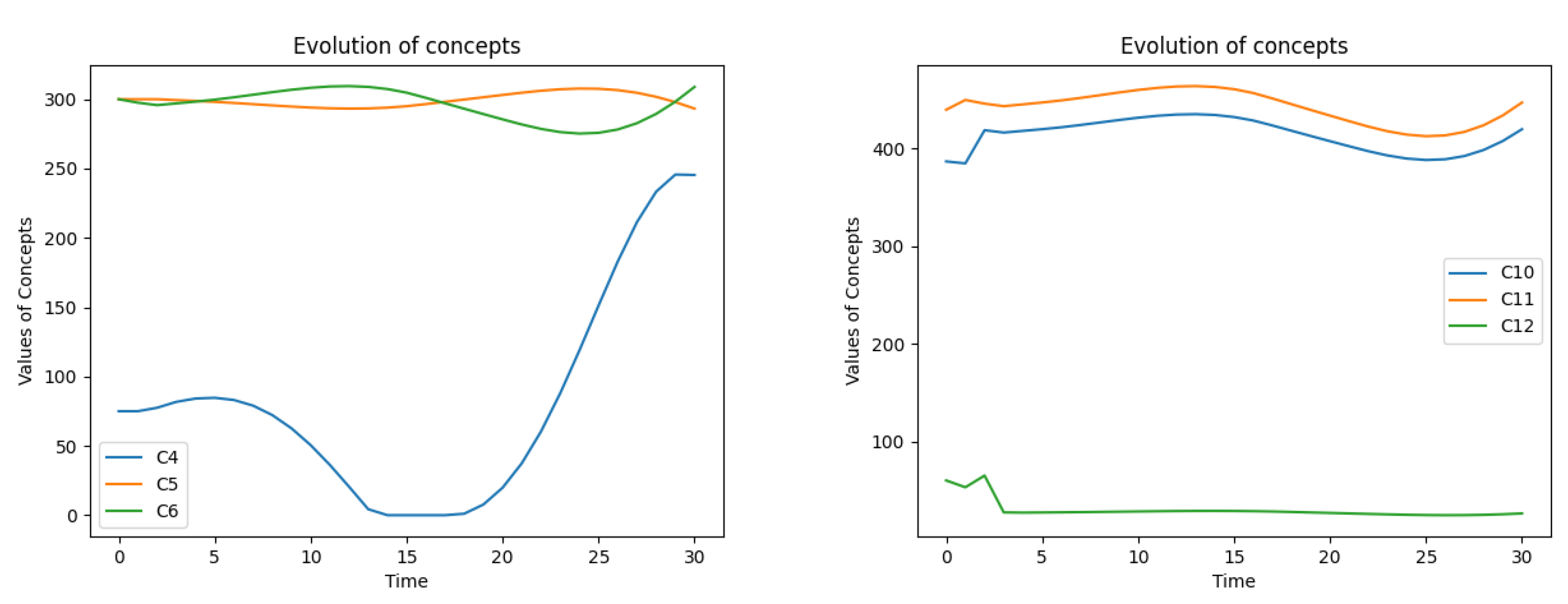
Figure 10 and Figure 11 illustrate the initial state of key system variables. A significant concern arises from the substantial increase in the service backlog between months 3 and 16, peaking almost 91 units in 7th month and drops to zero in 20th month (see Figure 11, left). This backlog surge is correlated with a 4% decline in customer numbers, from 100 to about 96 in 15th month, likely due to increased wait times Figure 10, left). The inadequate number of service employees (Figure 10, right) is identified as the root cause of the service backlog and subsequent customer loss. Income fluctuates within the range of 62-53 units, reaching the value of about 61 units in the 20th month (see Figure 11, right).
4.5.2. Scenario 1: Increased Hiring
To address the service backlog and customer loss, a potential intervention involves more aggressive hiring. By increasing the parameter from 0.03 to 0.039 (a 30% increase), coupled with raising the average salary to 2.2, we observe the following effects:
- The maximum backlog decreased to 85, reaching its peak earlier (at 5th month) and returning to zero sooner, in 15th month (see Figure 13, left).
- The decline in average customer numbers is slightly mitigated, reducing by about 2.5%, from a maximum of 100 to a minimum of 97.5 (see Figure 12, left).
- Employment rises to a higher level compared to the initial scenario, which contributes to the reduction in backlog.
- Income drops significantly, falling from an initial value of 60 to 28 units by the 10th month (see Figure 13, right)
Figure 12.
Scenario 1. The evolution of customers number C1 (left) and service employees number C7 (right).
Figure 12.
Scenario 1. The evolution of customers number C1 (left) and service employees number C7 (right).
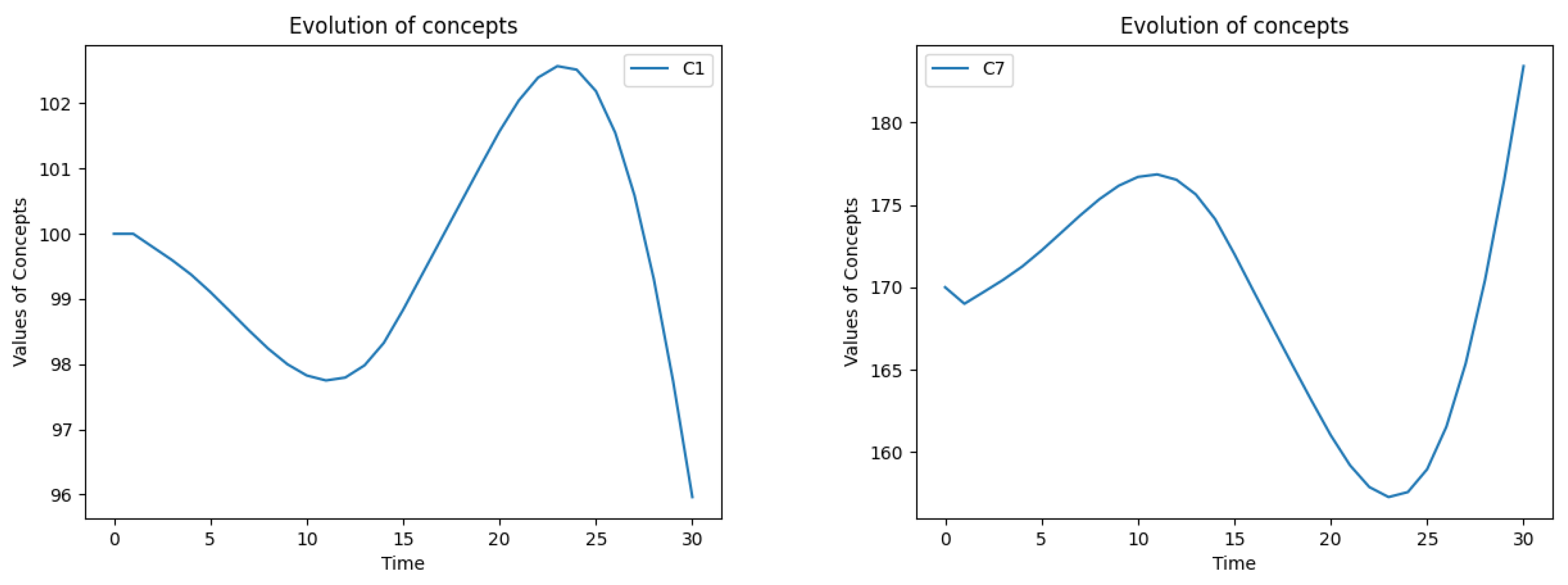
Figure 13.
Scenario 1. The evolution of: backlog C4 and its increase C5, decrease C6 (left), financial variables C10 – expenses, C11 – revenues, C12 – income (right).
Figure 13.
Scenario 1. The evolution of: backlog C4 and its increase C5, decrease C6 (left), financial variables C10 – expenses, C11 – revenues, C12 – income (right).
4.5.3. Scenario 2: Increased Training & Incentives Budget
An alternative scenario involves increasing the training and incentives budget. Company analysis indicated that doubling both training and incentives spending per employee in a coordinated manner is the optimal strategy. Smaller increases in these budgets produce less significant effects, while larger increases yield diminishing returns. This approach is expected to raise average productivity by approximately 12%. The resulting outcomes are as follows:
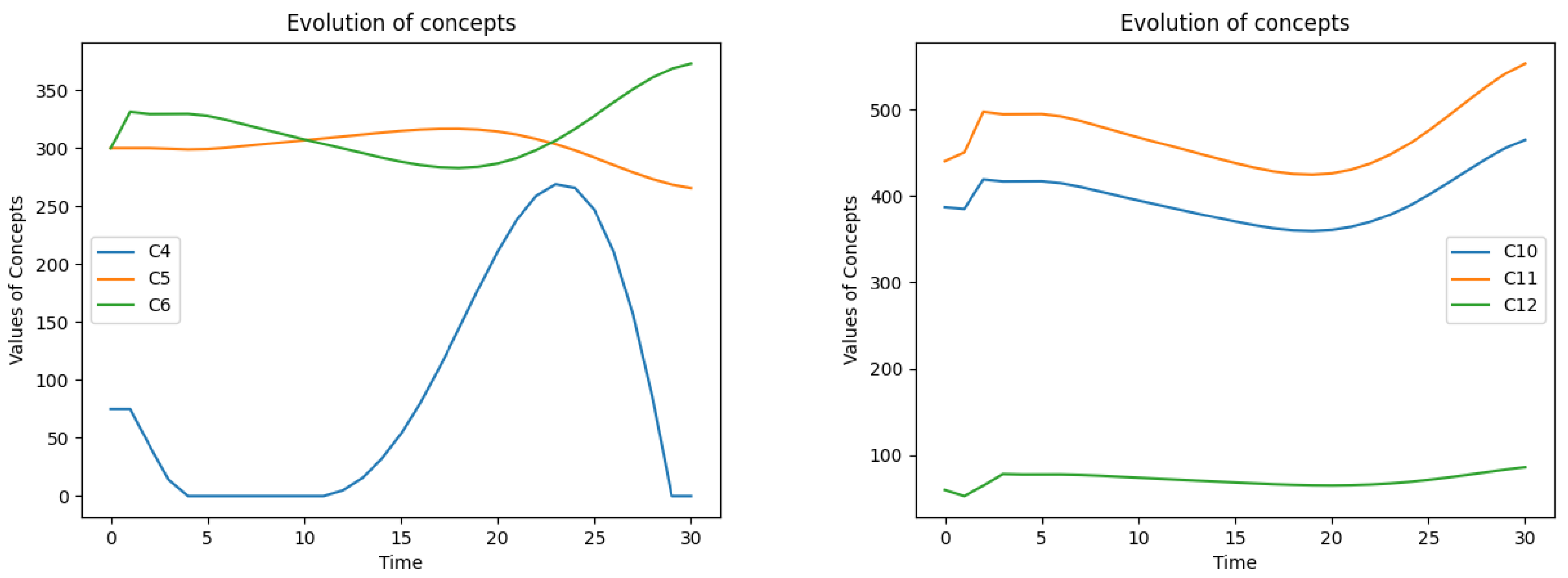
- The backlog begins to decrease immediately, reaching zero as early as the 4th month.
- The number of customers remains virtually stable, peaking at over 105 in the 17th month.
- Improved efficiency allows for a reduced workforce, with employee numbers declining to around 145 during the first 17 months.
- Income rises to about 78 units by the 6th month, then gradually declines to a range of 65–67 units between the 16th and 20th months.
Figure 14.
Scenario 2. The evolution of customers number C1 (left) and service employees number C7 (right).
Figure 14.
Scenario 2. The evolution of customers number C1 (left) and service employees number C7 (right).
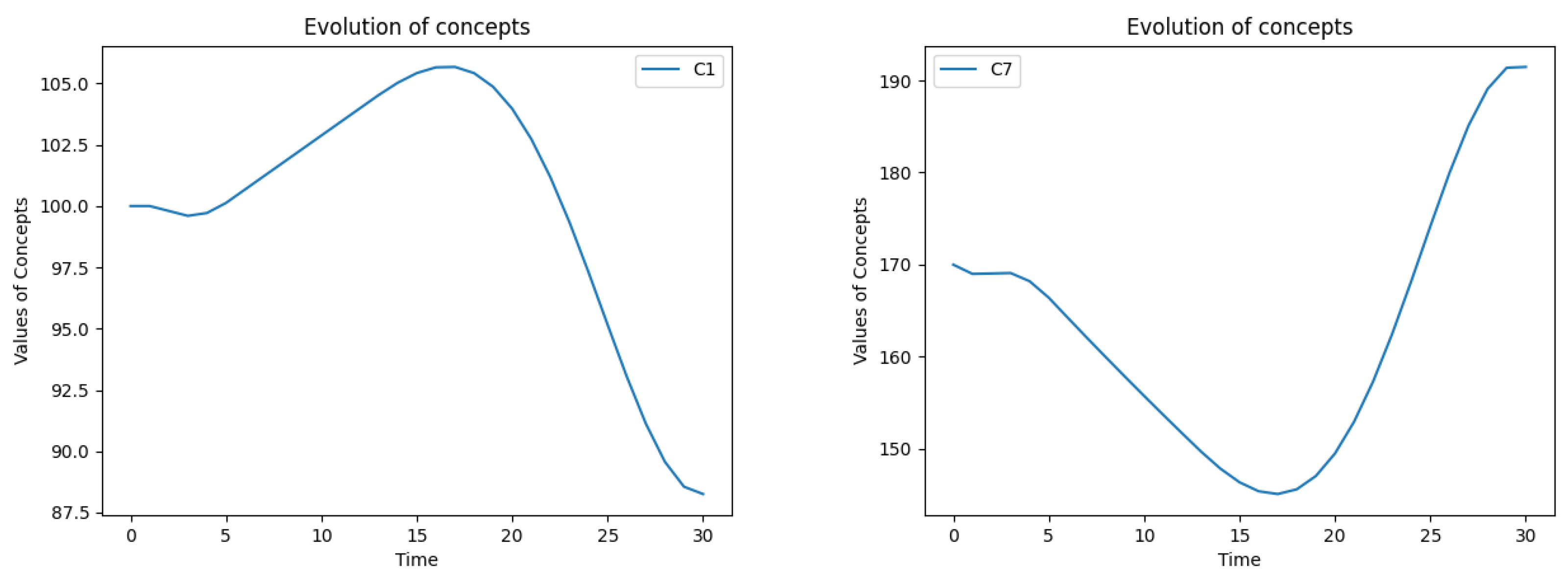
Figure 15.
Scenario 2. The evolution of: backlog C4 and its increase C5, decrease C6 (left), financial variables C10 – expenses, C11 – revenues, C12 – income (right).
Figure 15.
Scenario 2. The evolution of: backlog C4 and its increase C5, decrease C6 (left), financial variables C10 – expenses, C11 – revenues, C12 – income (right).
4.5.4. Validation and Sensitivity Analysis
Because this paper introduces a novel method, it is illustrated using simplified models. This prevents a comprehensive validation of these models (see e.g. [48]). Although the model described here refers to the same organization and its processes, and is also based on the Balanced Scorecard (BSC) like the one in [47], it is not identical, making a direct comparison of the results impossible. Nevertheless, qualitative similarities stemming from the conceptual resemblance of both models can be observed. In both models, fluctuations in the service backlog and the number of customers, among other things, can be seen. These become apparent at certain parameter values. Due to the different structure of the ’Growth and Learning’ submodel, the fluctuations in the number of employees that occur in this work are not visible in [47].
Initial validity tests, including extreme condition tests and degenerate tests consistent with methodology described by Sargent [48], confirm the robustness of the presented model. For instance, an increase in the customer growth rate () parameter leads to a proportional increase in the number of customers relative to the baseline. Similarly, a rise in the attrition rate () parameter results in reduced employment and an increase in the backlog. Conversely, when the customer growth rate () is set to zero, the model shows a continuous decline in the number of customers, accompanied by a drop in employment and revenue.
For the purpose of a sensitivity analysis, we will investigate the effect of changes to the key parameter, average productivity (), within a range of to . The resulting impact on the primary model variables is shown in Figure 16 and Figure 17. A qualitative analysis of the differences presented in these graphs, even without referring to the exact values, allows conclusions to be drawn.
At first glance, all variables behave rationally and in line with intuition. When productivity declines, the service backlog increases approximately in proportion to the magnitude of the drop. Conversely, higher productivity accelerates the reduction of the backlog and extends the period during which it remains at zero. A similar pattern holds for the number of customers: under a decline in productivity, the customer count contracts more rapidly with a 20% reduction than with a 10% reduction, and the trough is approximately proportional to the size of the decrease. When productivity rises, however, the increase in customer numbers is smaller than the decline observed under reduced productivity, and moving from +10% to +20% no longer yields a proportional effect. This suggests that productivity and backlog effects alone are insufficient to expand the customer base; additional measures, for example in marketing and sales, may be required. Employment likewise behaves as expected: when productivity falls, it rises roughly in proportion to the magnitude of the decline, whereas when productivity increases, it falls, albeit non-proportionally. Revenues, by contrast, vary approximately in proportion to changes in productivity in both directions; a 20% decline in productivity quickly leads to losses.
4.5.5. Simulations Summary
The results suggest that initiatives aimed at boosting productivity offer a more effective solution than aggressive employment policies. Naturally, such improvements cannot be pursued indefinitely; after several months, alternative approaches may become more advantageous. Additionally, other parameters can be adjusted and tested within the model. Overall, the complex interactions among factors underscore the potential for diverse intervention strategies, often requiring simultaneous adjustments across multiple parameters.
5. Conclusions and Future Research Directions
This paper introduced Algebraic Modeling of the Evolution of a System (ALMODES) as a discrete-time, matrix-based framework for simulating the evolution of social systems in sustainability contexts. By representing system structure as a directed graph and iterating the update by vector calculus, ALMODES reduces data requirements, keeps model structure transparent for stakeholders, and aligns with the discrete character of many social measurements. The approach remains compatible with other discrete paradigms and can be hybridized when greater behavioral detail is needed.
Across two illustrative studies—urban public health and a high-tech services firm—ALMODES supported diagnosis of feedbacks, staging of interventions, and comparison of strategic levers. In the public health example, the method reproduced intuitive long-run stabilization under adequate modernization and sanitation while revealing a plausible overcrowding failure mode with disease resurgence; strengthening the modernization–sanitation linkage mitigated this risk. In the firm-level Balanced Scorecard model, ALMODES made visible how workforce policies propagate through backlog, customer dynamics, and income. Scenario analysis and sensitivity tests converged on a practical insight: productivity-oriented investments (training and incentives) dampened fluctuations faster, stabilized customers, and improved income with fewer side effects than aggressive hiring alone. More broadly, the framework enabled rapid “what-if” exploration around human-capital stability—central to sustainable strategy in high-tech services.
Methodologically, ALMODES offers (i) an intuitive graph–algebra representation that facilitates participatory structuring; (ii) computational efficiency that scales as models grow; and (iii) straightforward avenues for scenario design, sensitivity analysis, and—via modest extensions—uncertainty handling. Limitations mirror those of other parsimonious system models: dependence on expert judgment for interaction strengths; under-representation of strong nonlinearities and threshold effects; and the need for systematic validation as scope increases. Nonetheless, matrix iteration scales favorably and, in practice, enables frequent re-estimation and re-simulation as new evidence arrives.
Future research directions:
- Uncertainty and robustness: introduce interval/fuzzy parameters and stochastic draws in the iteration; report distributions of outcomes and robustness envelopes.
- Hybrid models: couple ALMODES with agent-based modeling (heterogeneous actors) and discrete-event simulation (queues, resources) to capture micro-level mechanisms and operational constraints.
- Time-varying structures: allow to evolve with policy phases and shocks; study resilience under structural breaks.
- Estimation and validation: develop data-driven parameter estimation (e.g., regularized regression/Bayesian updating on panel time series), plus protocolized validity testing and benchmarking against system-dynamics models on shared cases.
- Control and optimization: embed multi-objective policy search (service, social, environmental, financial) and simple model-predictive control for rolling decision support.
- Participatory tooling: release open, documented software that turns digraphs into runnable ALMODES models with scenario dashboards to support stakeholder co-design.
- Sustainability metrics integration: link state variables to SDG-aligned indicators (equity, health, environmental load) to evaluate trade-offs and co-benefits explicitly.
Taken together, these steps would extend ALMODES from an accessible exploratory simulator into a robust, hybrid, and participatory platform for designing and stress-testing sustainable strategies in complex, evolving social systems.
Conflicts of Interest
The authors declare no conflicts of interest.
References
- Warfield, J.N. An assault on complexity,; Battelle, Office of Corporate Communications: Columbus, Ohio, 1973. [Google Scholar]
- Warfield, J.N. Structuring complex systems,; Battelle Memorial Institute: Columbus, Ohio, 1974. [Google Scholar]
- Sreenivasan, A.; Ma, S.; Nedungadi, P.; Sreedharan, V.R.; Raman, R.R. Interpretive Structural Modeling: Research Trends, Linkages to Sustainable Development Goals, and Impact of COVID-19. Sustainability 2023, 15, 4195. [Google Scholar] [CrossRef]
- Gabus, A.; Fontela, E. Perceptions of the world problematic: Communication procedure, communicating with those bearing collective responsibility. Technical report, Battelle Geneva Research Centre, Geneva, Switzerland, 1973.
- Fontela, E.; Gabus, A. The DEMATEL Observer. Technical report, Battelle Geneva Research Centre, Geneva, Switzerland, 1976.
- Wang, D.; Yan, L.; Ruan, F. A Combined IO–{DEMATEL} Analysis for Evaluating Sustainable Effects of the Sharing Related Industries Development. Sustainability 2022, 14, 5592. [Google Scholar] [CrossRef]
- Li, Y.; Zhao, G.; Wu, P.; Qiu, J. An Integrated Gray {DEMATEL} and ANP Method for Evaluating the Green Mining Performance of Underground Gold Mines. Sustainability 2022, 14, 6812. [Google Scholar] [CrossRef]
- Si, S.L.; You, X.Y.; Liu, H.C.; Zhang, P. DEMATEL Technique: A Systematic Review of the State-of-the-Art Literature on Methodologies and Applications. Mathematical Problems in Engineering 2018, 2018, 3696457. [Google Scholar] [CrossRef]
- Kumar, R.; Goel, P. Exploring the Domain of Interpretive Structural Modelling (ISM) for Sustainable Future Panorama: A Bibliometric and Content Analysis. Archives of Computational Methods in Engineering 2022, 29, 2781–2810. [Google Scholar] [CrossRef]
- Warfield, J.N. Binary Matrices in System Modeling. IEEE Transactions on Systems, Man, and Cybernetics 1973, SMC-3, 441–449. [Google Scholar] [CrossRef]
- Michnik, J. Weighted Influence Non-linear Gauge System (WINGS) - An analysis method for the systems of interrelated components. European Journal of Operational Research 2013, 536–544. [Google Scholar] [CrossRef]
- Kosko, B. Fuzzy cognitive maps. International Journal of Man-Machine Studies 1986, 24, 65–75. [Google Scholar] [CrossRef]
- Papageorgiou, K.; Singh, P.K.; Papageorgiou, E.; Chudasama, H.; Bochtis, D.; Stamoulis, G. Fuzzy Cognitive Map-Based Sustainable Socio-Economic Development Planning for Rural Communities. Sustainability 2020, 12, 305. [Google Scholar] [CrossRef]
- Gray, S.; Sterling, E.J.; Aminpour, P.; Goralnik, L.; Singer, A.; Wei, C.; Akabas, S.; Jordan, R.C.; Giabbanelli, P.J.; Hodbod, J.; et al. Assessing (Social–Ecological) Systems Thinking by Evaluating Cognitive Maps. Sustainability 2019, 11, 5753. [Google Scholar] [CrossRef]
- Papageorgiou, E.I. (Ed.) Fuzzy Cognitive Maps for Applied Sciences and Engineering: From Fundamentals to Extensions and Learning Algorithms, 2014th edition ed.; Springer: Berlin, Heidelberg, 2013. [Google Scholar]
- Godet, M. From Anticipation to Action: A Handbook of Strategic Prospective; United Nations Educational: Paris, France, 1994. [Google Scholar]
- Forrester, J.W. Industrial dynamics.; M.I.T. Press: Cambridge, Mass., 1961. [Google Scholar]
- Forrester, J.W. System dynamics, systems thinking, and soft OR. System Dynamics Review 1994, 10, 245–256. [Google Scholar] [CrossRef]
- Naeem, K.; Zghibi, A.; Elomri, A.; Mazzoni, A.; Triki, C. A Literature Review on System Dynamics Modeling for Sustainable Management of Water Supply and Demand. Sustainability 2023, 15, 6826. [Google Scholar] [CrossRef]
- Morecroft, J.D.W. Strategic Modelling and Business Dynamics, + Website: A feedback systems approach, 2 edition ed.; Wiley: Hoboken, New Jersey, 2015. [Google Scholar]
- Sterman, J. Business Dynamics: Systems Thinking and Modeling for a Complex World; Irwin/McGraw-Hill, 2000. [Google Scholar]
- Fonseca, L.; Carvalho, F.; Santos, G. Strategic CSR: Framework for Sustainability Through Management Systems Standards—Implementing and Disclosing Sustainable Development Goals and Results. Sustainability 2023, 15, 11904. [Google Scholar] [CrossRef]
- Giddings, B.; Hopwood, B.; O’Brien, G. Environment, economy and society: fitting them together into sustainable development. Sustainable Development 2002, 10, 187–196. [Google Scholar] [CrossRef]
- OECD. Strategies for Sustainable Development, The DAC Guidelines. Technical report; OECD Publishing: Paris, 2001. [Google Scholar]
- Biermann, F.; Hickmann, T.; Sénit, C.A.; Beisheim, M.; Bernstein, S.; Chasek, P.; Grob, L.; Kim, R.E.; Kotzé, L.J.; Nilsson, M.; et al. Scientific evidence on the political impact of the Sustainable Development Goals. Nature Sustainability 2022, 5, 795–800. [Google Scholar] [CrossRef]
- Mishra, M.; Desul, S.; Santos, C.A.G.; Mishra, S.K.; Kamal, A.H.M.; Goswami, S.; Kalumba, A.M.; Biswal, R.; da Silva, R.M.; dos Santos, C.A.C.; et al. A bibliometric analysis of sustainable development goals (SDGs): a review of progress, challenges, and opportunities. Environment, Development and Sustainability 2024, 26, 11101–11143. [Google Scholar] [CrossRef]
- Krellenberg, K.; Bergsträßer, H.; Bykova, D.; Kress, N.; Tyndall, K. Urban Sustainability Strategies Guided by the SDGs—A Tale of Four Cities. Sustainability 2019, 11, 1116. [Google Scholar] [CrossRef]
- Salvador, M.; Guijarro, M.; Valdivieso-Álvarez, M.; Rodríguez, A. The Role of Local Government in the Drive for Sustainable Development Public Policies: An Analytical Framework Based on Institutional Capacities. Sustainability 2021, 13, 5978. [Google Scholar] [CrossRef]
- Teixeira, T.B.; Battistelle, R.A.G.; Teixeira, A.A.; Mariano, E.B.; Moraes, T.E.C. The Sustainable Development Goals Implementation: Case Study in a Pioneer Brazilian Municipality. Sustainability 2022, 14, 12746. [Google Scholar] [CrossRef]
- Kumar, P.; Sahani, J.; Corada Perez, K.; Ahlawat, A.; Andrade, M.d.F.; Athanassiadou, M.; Cao, S.J.; Collins, L.; Dey, S.; Di Sabatino, S.; et al. Urban greening for climate resilient and sustainable cities: grand challenges and opportunities. Frontiers in Sustainable Cities 2025, 7. [Google Scholar] [CrossRef]
- Richiedei, A.; Gollini, I.; Congiu, T.; Ostanello, D. Territorializing and Monitoring of Sustainable Development Goals in Italy: An Overview. Sustainability 2022, 14, 3056. [Google Scholar] [CrossRef]
- Ding, Z.; Gong, W.; Li, S.; Wu, Z. System Dynamics versus Agent-Based Modeling: A Review of Complexity Simulation in Construction Waste Management. Sustainability 2018, 10, 2484. [Google Scholar] [CrossRef]
- Peretz, H. Sustainable Human Resource Management and Employees’ Performance: The Impact of National Culture. Sustainability 2024, 16, 7281. [Google Scholar] [CrossRef]
- Madero-Gómez, S.M.; Rubio Leal, Y.L.; Olivas-Luján, M.; Yusliza, M.Y. Companies Could Benefit When They Focus on Employee Wellbeing and the Environment: A Systematic Review of Sustainable Human Resource Management. Sustainability 2023, 15, 5435. [Google Scholar] [CrossRef]
- Florek-Paszkowska, A.; Hoyos-Vallejo, C.A. Going green to keep talent: Exploring the relationship between sustainable business practices and turnover intention. Journal of Entrepreneurship, Management and Innovation 2023, 19, 87–128. [Google Scholar] [CrossRef]
- Kotłowska, A. The Shortened Working Week and Its Impact on Workplace Sustainability. Edukacja Ekonomistów i Menedżerów : problemy, innowacje, projekty 2024, 71, 69–97. [Google Scholar] [CrossRef]
- Nguyen, L.K.N.; Howick, S.; Megiddo, I. A framework for conceptualising hybrid system dynamics and agent-based simulation models. European Journal of Operational Research 2024, 315, 1153–1166. [Google Scholar] [CrossRef]
- Morgan, J.S.; Howick, S.; Belton, V. A toolkit of designs for mixing Discrete Event Simulation and System Dynamics. European Journal of Operational Research 2017, 257, 907–918. [Google Scholar] [CrossRef]
- Chahal, K.; Eldabi, T. WHICH IS MORE APPROPRIATE : A MULTI-PERSPECTIVE COMPARISION BETWEEN SYSTEM DYNAMICS AND DISCRETE EVENT SIMULATION. 2008.
- Michnik, J. Algebraic Modeling of Social Systems Evolution – ALMODES, Banja Koviljača, Serbia, 2021; pp. 641–646. https://symopis2022.ekof.bg.ac.rs/download/istorijat/XLVIII_Simpozijum_o_operacionim_istrazivanjima.pdf.
- Maruyama, M. THE SECOND CYBERNETICS Deviation-Amplifying Mutual Causal Processes. American Scientist 1963, 5, 164–179. [Google Scholar]
- Tsadiras, A.K.; Margaritis, K.G. Cognitive mapping and certainty neuron fuzzy cognitive maps. Information Sciences 1997, 101, 109–130. [Google Scholar] [CrossRef]
- Kaplan, R.S.; Norton, D.P. The Balanced Scorecard—Measures that Drive Performance. Harvard Business Review 1992. [Google Scholar]
- Kaplan, R.S. Conceptual Foundations of the Balanced Scorecard. Harvard Business School Accounting & Management Unit Working Paper 10-074, Harvard Business School, Boston, MA, 2010.
- Kumar, S.; Lim, W.M.; Sureka, R.; Jabbour, C.J.C.; Bamel, U. Balanced scorecard: trends, developments, and future directions. Review of Managerial Science 2023, 18, 2397–2439. [Google Scholar] [CrossRef]
- Madsen, D.O. Balanced Scorecard: History, Implementation, and Impact. Encyclopedia 2025, 5, 39. [Google Scholar] [CrossRef]
- Banaś, D.; Michnik, J.; Targiel, K. System modeling and control of organization business processes by use of balanced scorecard and system dynamics. Control and Cybernetics 2016, 185–205. [Google Scholar]
- Sargent, R.G. Verification and validation of simulation models. In Proceedings of the Proceedings of the 2010 Winter Simulation Conference, 2010; pp. 166–183. [Google Scholar] [CrossRef]
Figure 1.
An example graph of a system.
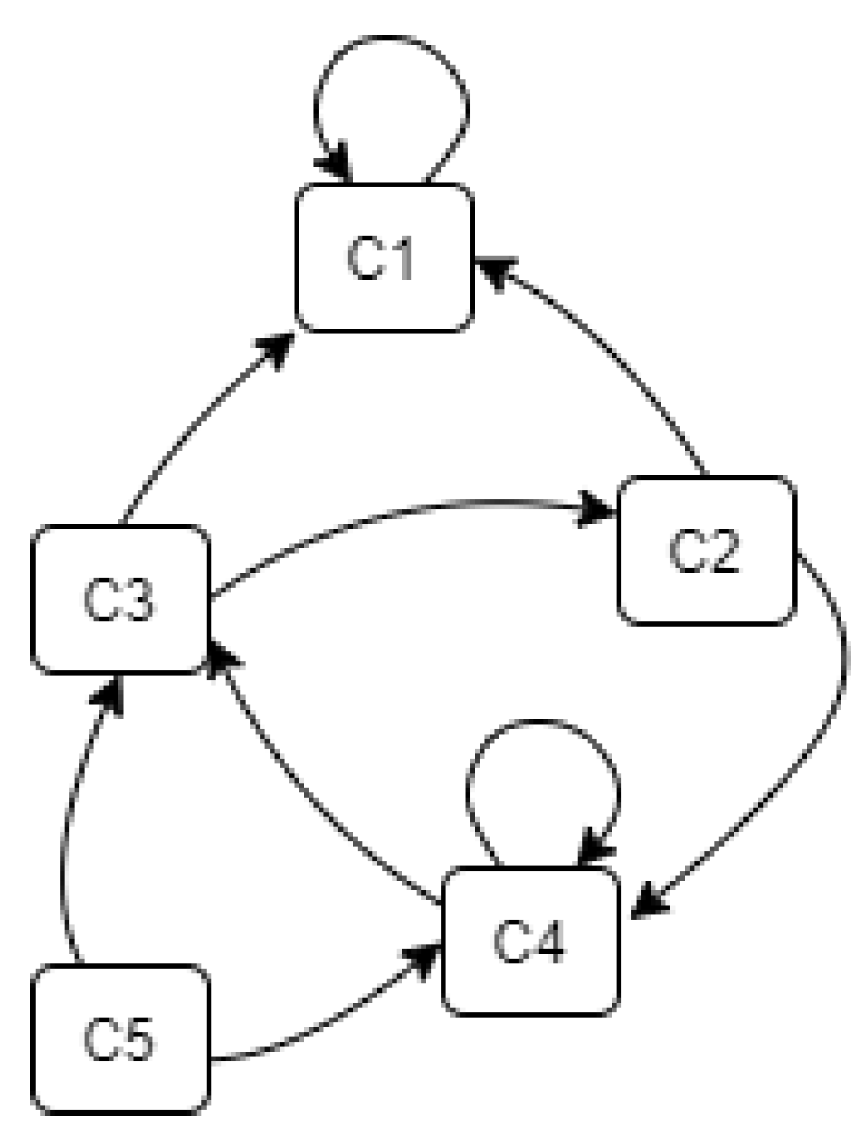
Figure 2.
The two-factor system—causal loop and its simulation as a balancing loop.
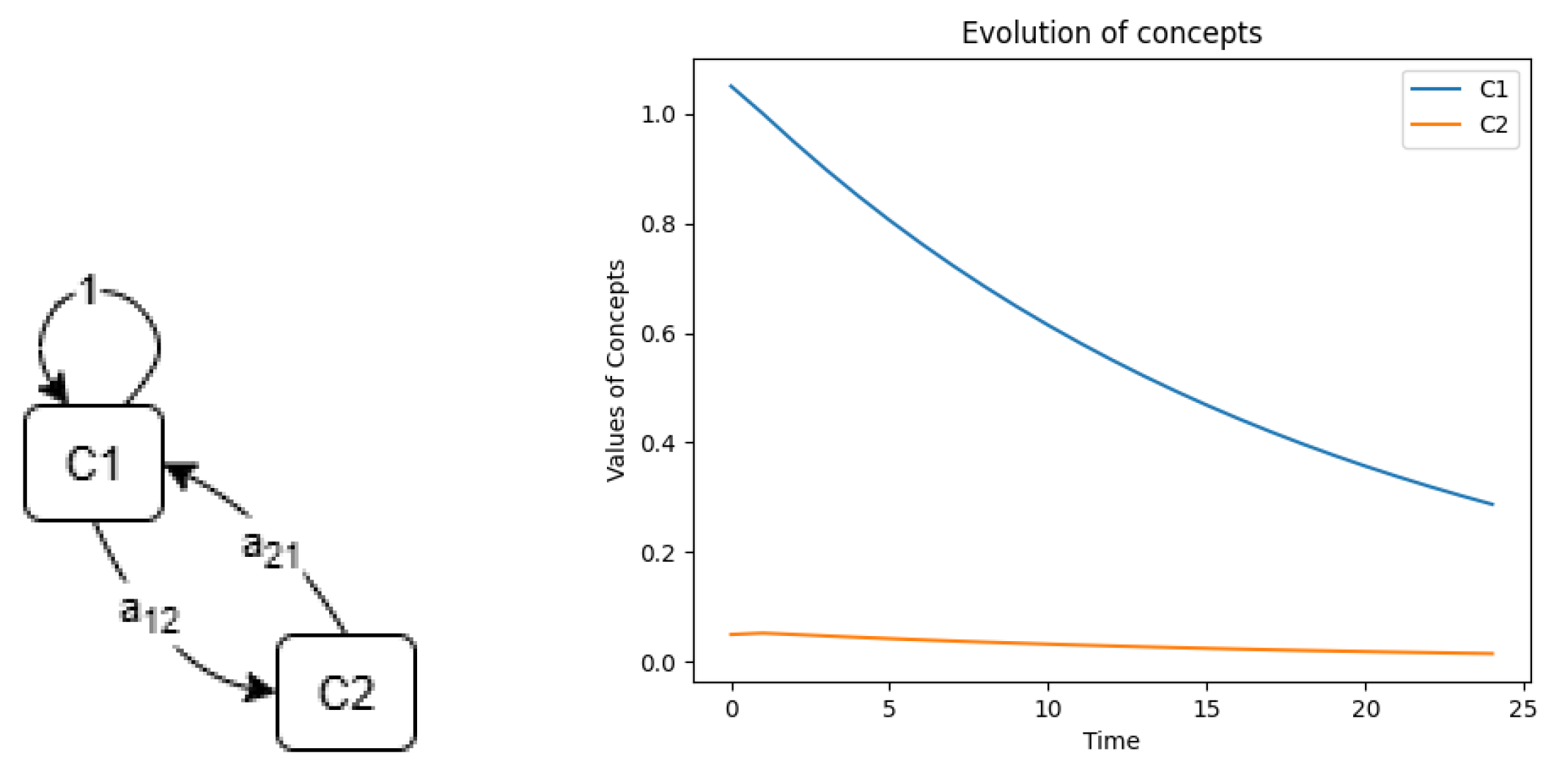
Figure 3.
Model of a container (matrix Eq. (4)) and its simulation (, and ).
Figure 3.
Model of a container (matrix Eq. (4)) and its simulation (, and ).
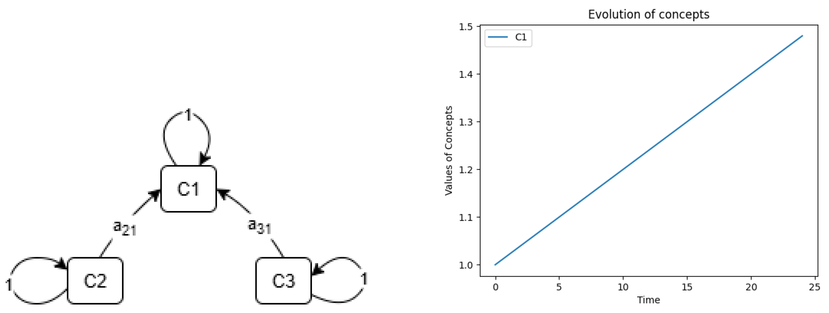
Figure 4.
Model of population (matrix: Eq. (6)) and its simulation (, and ).
Figure 4.
Model of population (matrix: Eq. (6)) and its simulation (, and ).
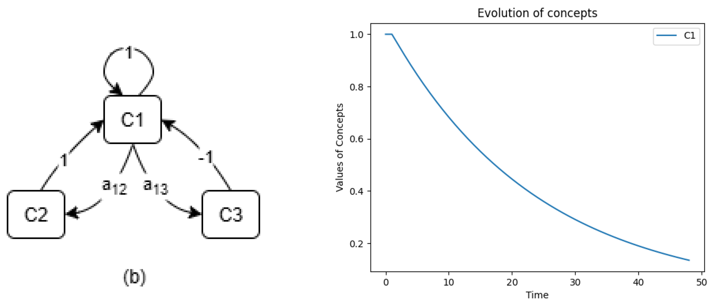
Figure 5.
ALMODES map of a public health system.
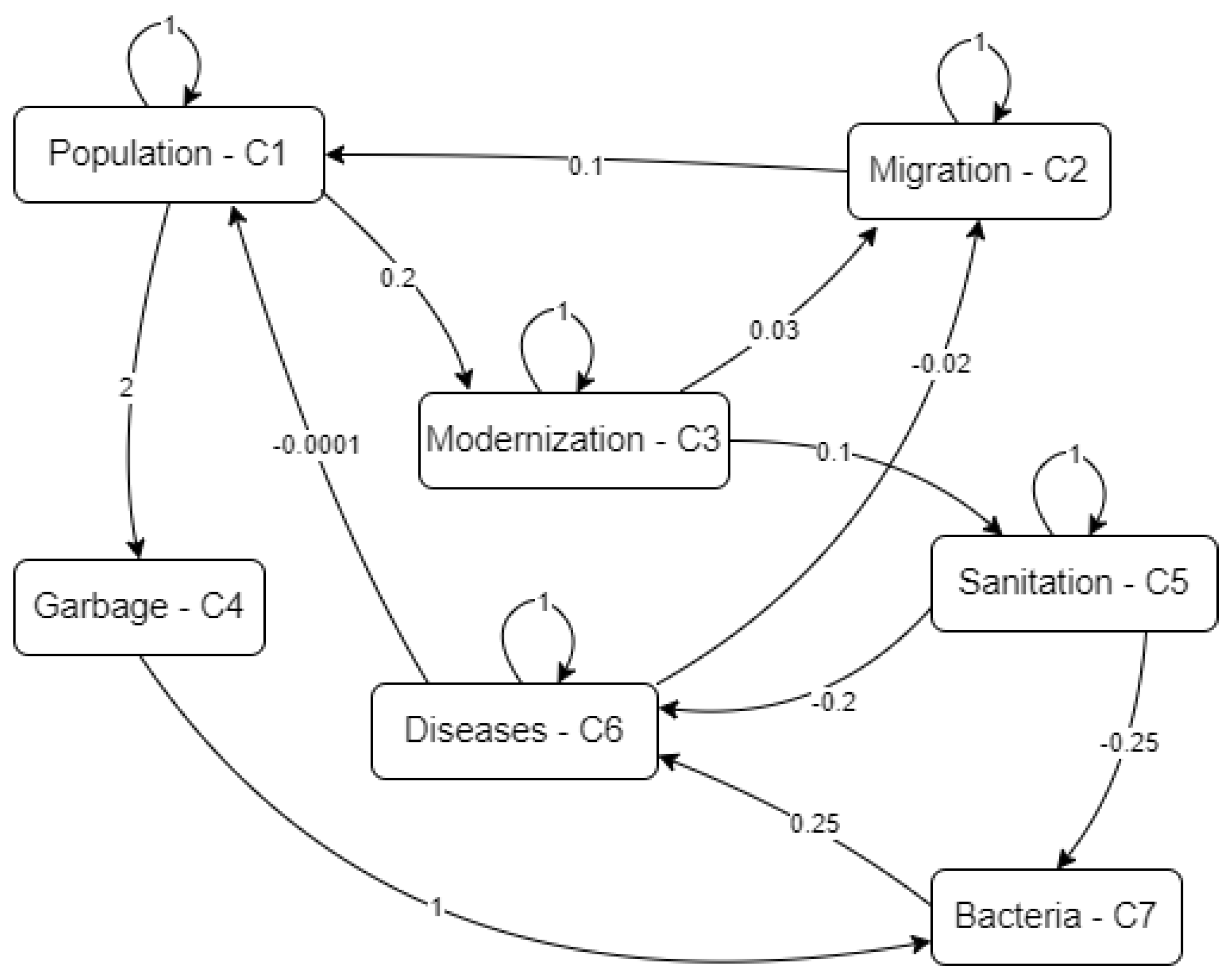
Figure 6.
Evolution of concepts in the public health model.
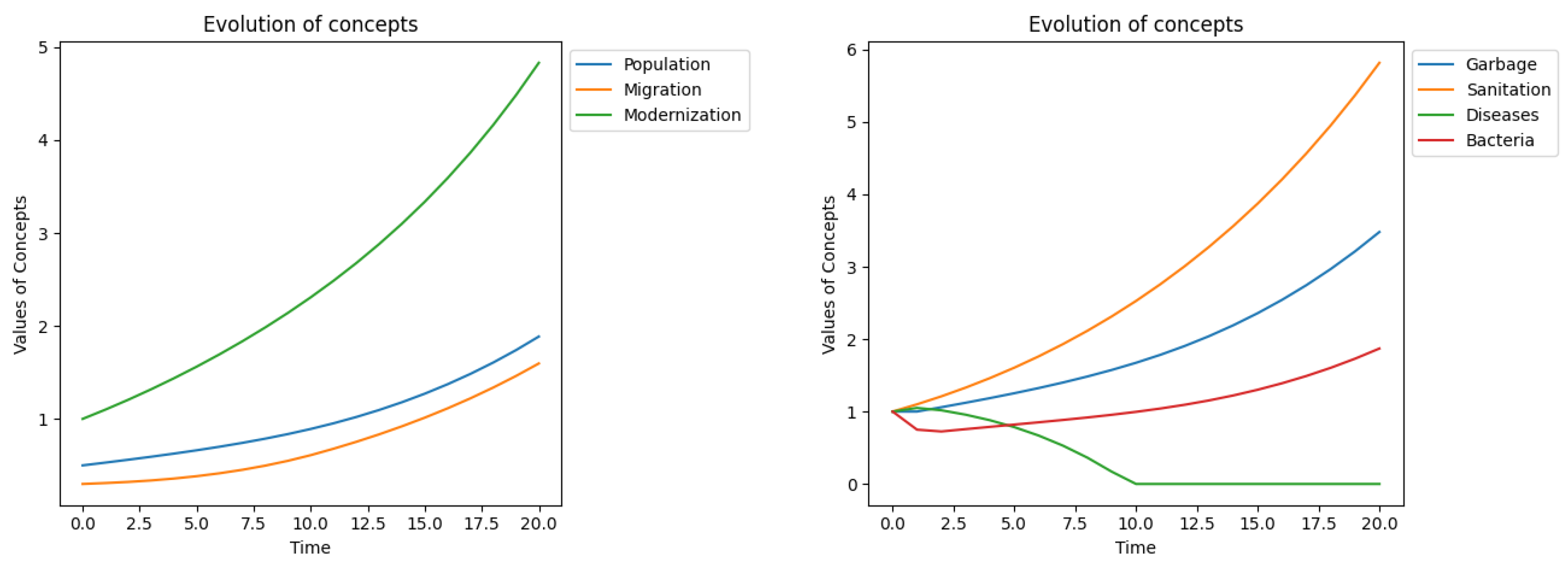
Figure 7.
Evolution of concepts in the public health model—overcrowded city.
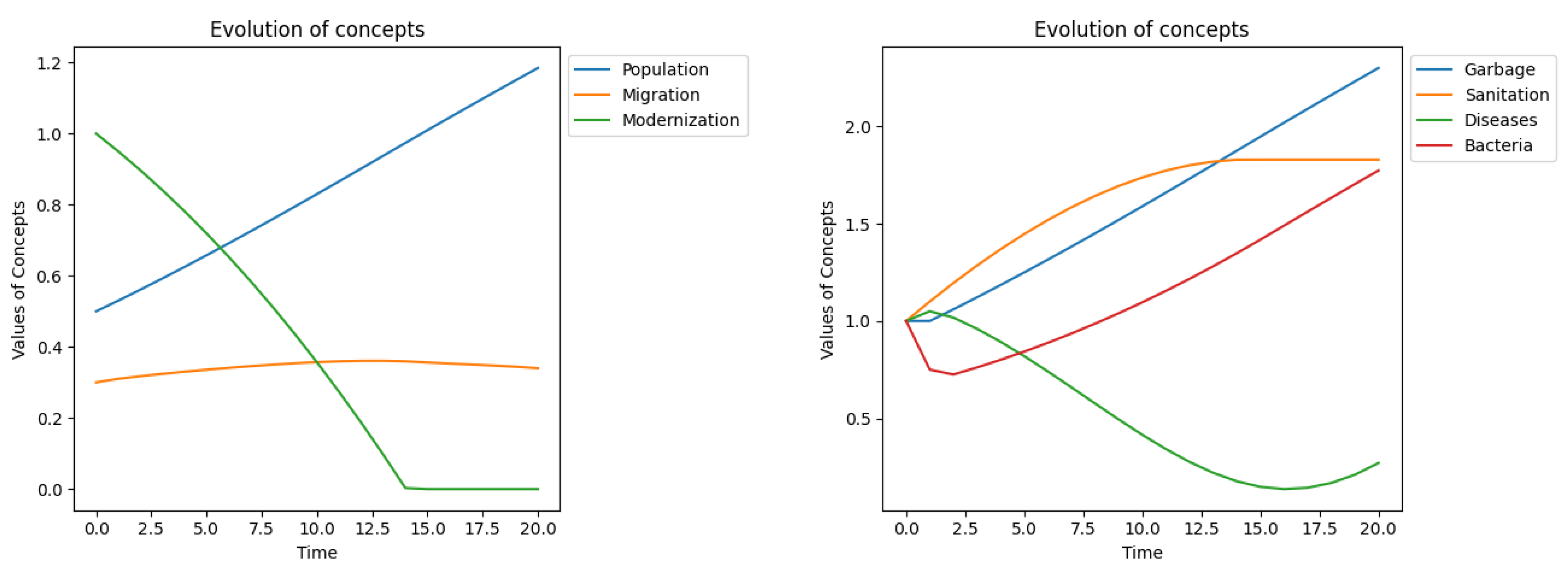
Figure 8.
Impact of potential intervention in an overcrowded city.
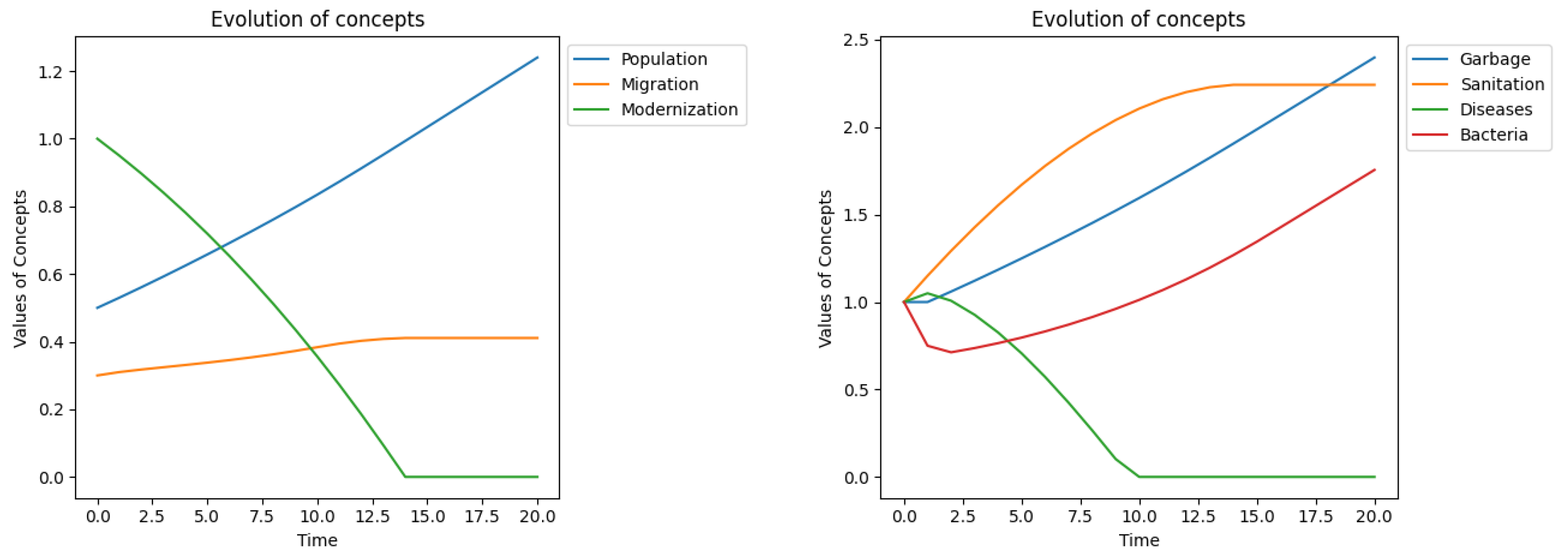
Figure 9.
The BSC model.
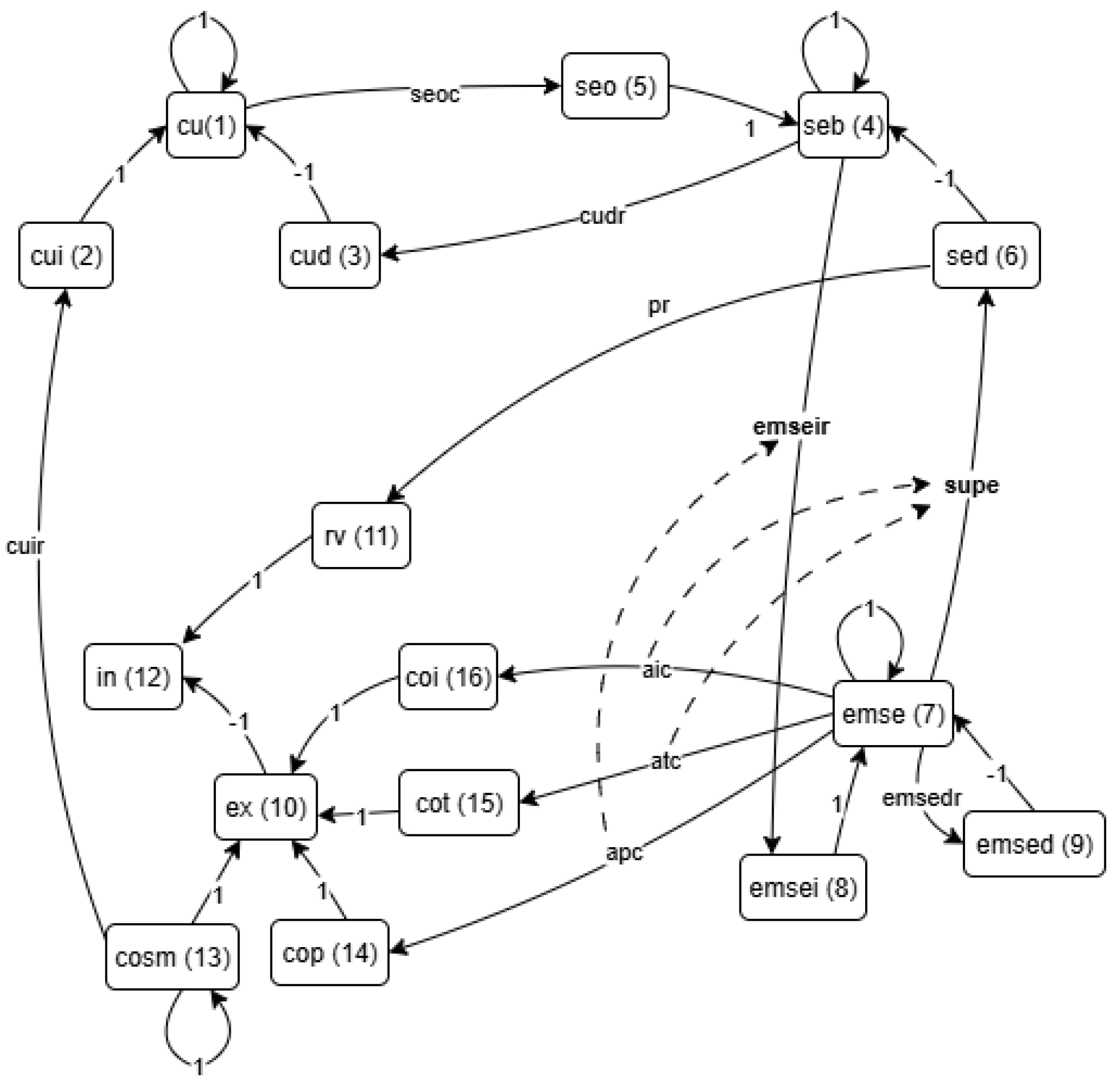
Figure 10.
Initial state. The evolution of customers number C1 (left) and service employees number C7 (right).
Figure 10.
Initial state. The evolution of customers number C1 (left) and service employees number C7 (right).
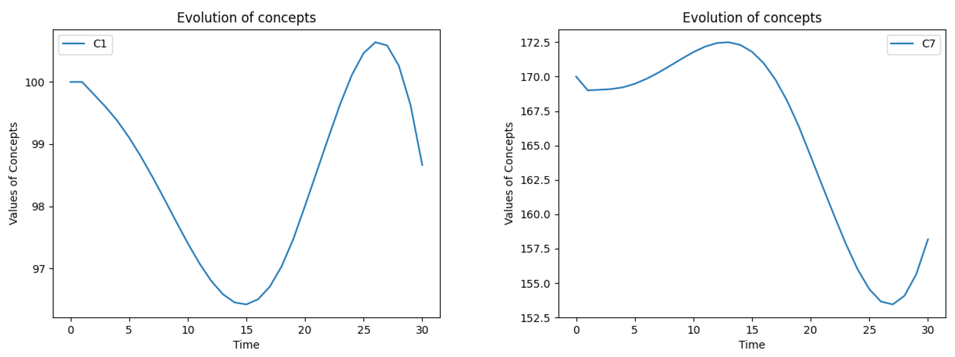
Figure 11.
Initial state. The evolution of: backlog C4 and its increase C5, decrease C6 (left), financial variables C10 – expences, C11 – revenues, C12 – income (right).
Figure 11.
Initial state. The evolution of: backlog C4 and its increase C5, decrease C6 (left), financial variables C10 – expences, C11 – revenues, C12 – income (right).
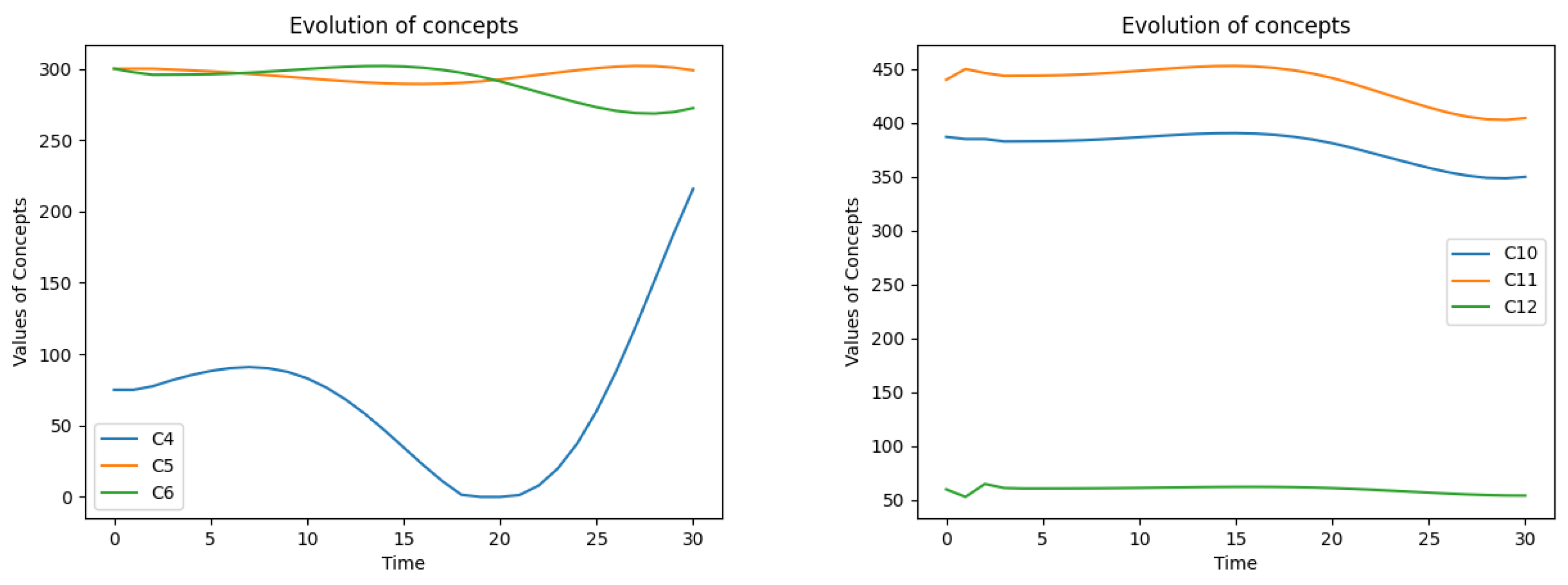
Figure 16.
Change of customers number (left) and change of service employees number C7 (right) caused by change of average productivity ()
Figure 16.
Change of customers number (left) and change of service employees number C7 (right) caused by change of average productivity ()
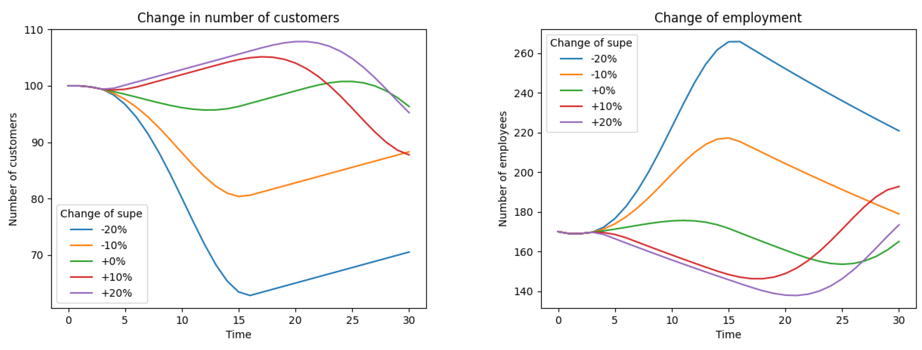
Figure 17.
Change in service backlog (left) and change in income (right) caused by change of average productivity ().
Figure 17.
Change in service backlog (left) and change in income (right) caused by change of average productivity ().
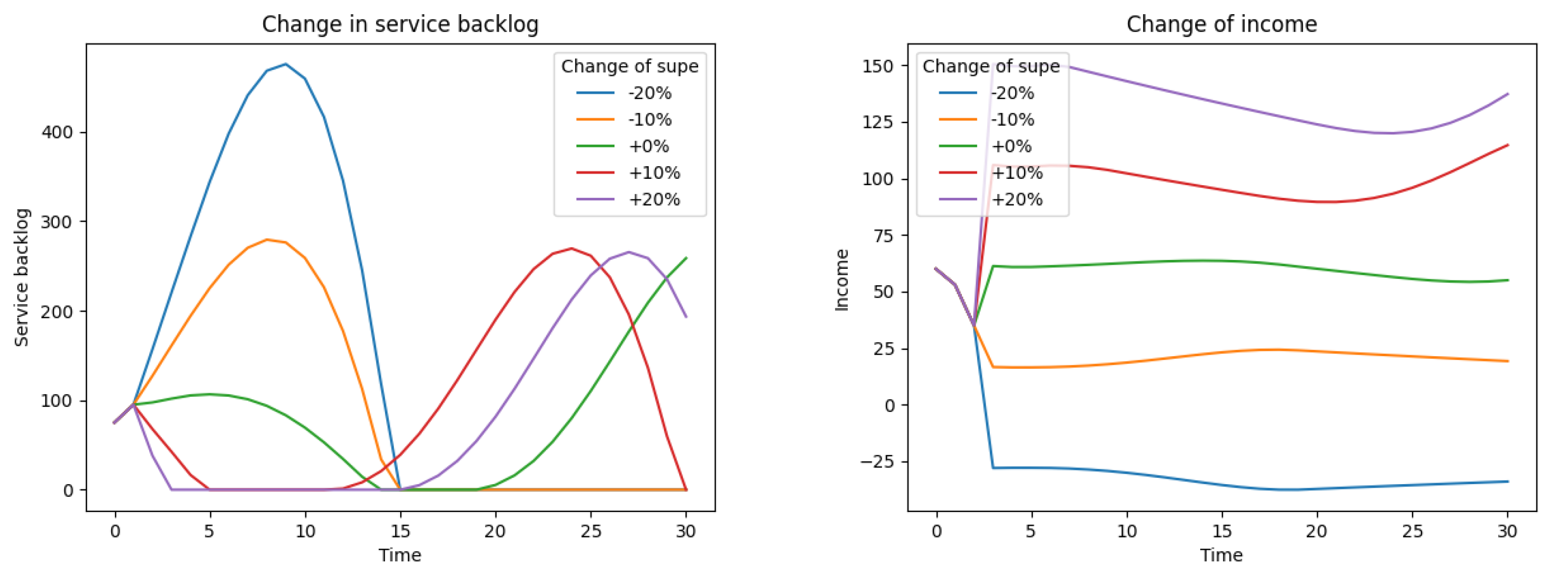

Table 1.
The concepts in the public health model.
| Concept | Unit | Initial value |
|---|---|---|
| C1 Population of a City | [100 000] | 0.5 |
| C2 Migration into a City | [10 000] | 0.3 |
| C3 Modernization | [conventional] | 1 |
| C4 Garbage per Area | [25 000 t] | 1 |
| C5 Sanitation Facilities | [conventional] | 1 |
| C6 Number of Diseases per 1000 Residents | [100] | 1 |
| C7 Bacteria per Area | [conventional] | 1 |
Disclaimer/Publisher’s Note: The statements, opinions and data contained in all publications are solely those of the individual author(s) and contributor(s) and not of MDPI and/or the editor(s). MDPI and/or the editor(s) disclaim responsibility for any injury to people or property resulting from any ideas, methods, instructions or products referred to in the content. |
© 2025 by the author. Licensee MDPI, Basel, Switzerland. This article is an open access article distributed under the terms and conditions of the Creative Commons Attribution (CC BY) license (http://creativecommons.org/licenses/by/4.0/).
Copyright: This open access article is published under a Creative Commons CC BY 4.0 license, which permit the free download, distribution, and reuse, provided that the author and preprint are cited in any reuse.


