
Submitted:
10 March 2025
Posted:
11 March 2025
You are already at the latest version
Abstract
It is known that the input-output model is based on the balance of inter-industry linkages, however, these conditions do not ensure equilibrium transactions among its agents, both producers and consumers. To address this issue, this work focuses on creating, justifying, and computational models for determine equilibrium transactions within the platform industry and ecosystems of Kazakhstan's financial and insurance activities industry. The research employs a conceptual design for computational models, integrating input (produce/selling, payments, imports) and output (purchase/buying, final demand, exports) transactions to analyze equilibrium growth in platform industries and ecosystems using OECD data from Kazakhstan's statistics (1995–2018). The main results of this study include computational models for determine equilibrium within the platform industry and its ecosystems of Kazakhstan's financial and insurance activities. Their application involves identifying time phases of undervalued and overvalued transactions, classifying time phases by their alignment with equilibrium transactions within the domain of feasible solutions, and analyzing the dynamics of equilibrium growth, enabling more efficient resource allocation and promoting sustainable growth for the industry and its ecosystem.
Keywords:
computational models
; equilibrium growth
; sustainable development
; financial and insurance activities
; Kazakhstan
1. Introduction
The incorporation of intelligent systems and sophisticated econometric models into the insurance and financial sectors has accelerated in recent years, driven by advancements in IoT, cloud computing, and machine learning. For example, Yu et al [1] developed a hierarchical game model to optimize job offloading in IoT-Edge-Cloud systems, while Zhang et al [2] introduced a blind post-decision state-based reinforcement learning (b-PDS) to improve decision-making efficacy. Furthermore, Huang [3] highlighted the relevance of IoT in enhancing logistics systems, demonstrating its capacity to improve efficiency within financial ecosystems.
The importance of sustainable development and balanced growth in the financial and insurance sectors of Kazakhstan has been extensively discussed. Daniya and Tang [4] studied the impact of green finance on the transition to a low-carbon economy, and Serkebayeva et al [5] analyzed liquidity issues in country’s stock market.
The insurance industry has also attracted the attention of researchers. Tasdemir and Alsu [6] analyzed the relationship between insurance activity and economic growth in G-20 countries, while Ahn and Park [7] showed the impact of corporate social responsibility (CSR) in the insurance sector on sustainable development. In addition, Avazov et al [8] noted the important role of investment activities in the insurance sector in shaping financial markets.
Technological advances are a significant factor in the development of financial analysis and decision-making processes. Lei et al [9] and Chou et al [10] proposed intelligent systems based on machine learning methods and metaheuristic optimization to improve the accuracy of financial forecasting results. The results achieved in this area were deeply studied in the scientific papers of Zhong and Fan [11] using cloud algorithms for optimizing corporate financial decisions, while Chen [12] was able to improve the accuracy by using the association rule search method in processing big data in the financial direction.
In this regard, the research below provides important concepts for developing the methods for studying equilibrium and growth models. Balbus et al [13] in their studies analyzed models of economic growth that take into account the interests of society and are based on mutual support among society, while Georgescu and Zhang [14] studied the long-term stability and coexistence of several economic agents or systems in logistic growth models. Thus, Jung [15], using a general equilibrium model, studied changes in the labor market from the perspective of the impact of skill diversity and skill levels of the workforce.
The extensive ramifications of these advances are seen in Shinozaki's research [16] regarding the influence of digital finance on small enterprises amid economic instability. Guo [17] and Liu [18] augmented the literature by introducing interactive systems for financial data analysis, highlighting real-time decision support.
The work of Balbus et al [13] on intergenerational growth and Svoboda and Fischer [19] on non-equilibrium thermodynamic models extends these frameworks to dynamic systems analysis. Both of these studies concern the analysis of dynamic systems. Last but not least, Li [20] and Zhong and Fan [11] demonstrated the significance of big data and genetic algorithms in the realm of financial control and investment decision-making, underlining the fact that these technologies are applicable to countries ever-evolving capital market environment.
More advanced computational methods and data-driven methodologies will make intelligent systems increasingly valuable for assessing the scope of balanced development of the insurance and financial sectors. Since financial systems are inherently complex and volatile, effective decision-making approaches must combine technical and economic knowledge. When asked about ways to improve operational efficiency and allocate resources more effectively, they mentioned deep learning and clustering. Several studies have investigated these intersections, providing both practical frameworks and theoretical advances. For example, Wang [21] and Song et al [22] demonstrated how intelligent analysis frameworks based on project and engineering management can optimize decision-making for regional economic development, emphasizing the utility of clustering algorithms and deep learning techniques in improving operational efficiency and resource allocation. Similarly, Farooq et al [23] employed input-output analysis to estimate the economic impact of Intelligent Transportation Systems (ITS), giving a methodology that may be adapted to financial ecosystems for assessing inter-industry effects [20].
To address the potential financial effects of renewable energy on profitability and operational expenditures, Suresh and Jagatheeswari [24] developed a smart grid-based hybrid intelligent optimization system. Consistent with the findings of Li's [20] study on financial big data control, this provides support for the notion that intelligent systems ought to be included in economic and environmental decision-making. Zhang et al [25] extended the employment of hybrid models by examining economic data using Long Short-Term Memory (LSTM) networks and showing that their predicted accuracy was better than that of conventional approaches like ARIMA and SVM.
Moreover, Deshkar's [26] economic modeling of the world cities with deep shallow learning networks and optimization algorithms shows the extensive applicability of intelligent systems to urban financial management. He [27] supports this by constructing a hybrid methodology for studying inequalities in economic development, emphasizing the contribution of machine learning in curbing regional growth imbalances.
Such studies quoted collectively emphasize the adaptability of intelligent systems in financial analysis, varying from project management to city economic forecasting. Nevertheless, such studies sometimes concentrate more on technical efficiency or industry insights and thus fall short in the integration of such systems in inclusive equilibrium growth models for the insurance and financial sectors. Therefore, we stated the following features of the systematization of scientific research and development:
- -
- -
- -
- -
- Partial integration in financial sectors, – most research has had general or sector-specific applications, with less focus on equilibrium growth analysis for financial and insurance sectors specifically;
- -
- Scalability issues, – some frameworks, particularly those built on complex algorithms, may experience difficulties if expanded to national or sectoral levels, as He [27] points out.
This research seeks to address these limitations by developing an intelligent system for equilibrium growth analysis in Kazakhstan's financial and insurance sectors, drawing from the strengths of existing studies to build a comprehensive, integrative framework.
Thus, the purpose of this study is to create, justify and apply an algorithm of the algorithms for determine equilibrium transactions of the platform industry and its ecosystems of Kazakhstan's financial and insurance activities industry. To achieve the purpose of this work we plan to present the research in the following sequence: Introduction (Section 1); Materials and methods: Conceptual design of the an algorithm for analyzing equilibrium growth (Section 2.1), Data, indicators and equilibrium transaction definition for the platform and its ecosystems (Section 2.1); Results: An algorithm to determine the equilibrium on the platform industry and its application (Section 3.1), An algorithm to determine the equilibrium on the internal ecosystem and its application (Section 3.2), An algorithm to determine the equilibrium on the external ecosystem and its application (Section 3.3); Discussion (Section 4); and Conclusions (Section 5).
2. Materials and Methods
2.1. Conceptual Design of Computational Modelling of Equilibrium Growth
Section 2.1 presents the conceptual design of computational modelling for analyzing equilibrium growth in the platform industry and its ecosystem. It emphasizes the role of total input and total output transactions in managing resource-commodity and nominal-monetary flows. In particular, according to [28], we combine the design of computational modelling at the input platform produce/selling, payments and import, and at the output platform purchase/buying, final demand, and export agents. Next, we explore the problem of organizing transaction flows between structures from the point of view of effective support of the technological chain in ensuring equilibrium growth in the platform industry and its ecosystem.
Platform industry – economic activity based on an intelligent information system, providing complex standard solutions for the hold and management of transactions of both resource-commodity and nominal-monetary values between agents of the platform and of the ecosystem.
The concept of computational modelling for analyzing the equilibrium growth of the platform industry consists of a block of the total input (see Figure 1a) and a block of the total output (see Figure 1b), as well as flows of resource-commodity values (see solid line of Figure 1) and nominal-monetary values (see dotted line of Figure 1) between the agents of the platform and the ecosystem [28]:
- -
- A block of the total input is based on platform produce/selling, internal ecosystem: payments and external ecosystem: import agents (see Figure 1a);
- -
- Resource-commodity values of the total input of the industry consist of the platform produce/selling, internal ecosystem payments, and external ecosystem imports transactions sum (see Figure 1a), i.e.
Total input = Produce/selling + Payments + Imports;
- -
- A block of the total output is based on platform purchase/buying, internal ecosystem final demand, and external ecosystem export agents (see Figure 1b);
- -
Total output = Purchase/buying + Final demand + Exports.
Thus, based on the received nominal-monetary values from the total output of the industry as feedback (see the dotted line between Figure 1a and Figure 1b) total input agents based on the distribution of resource-commodity values organize and manage the technological chain obtaining products for formations of values on the total output agents (see solid line between Figure 1a and Figure 1b). Then a necessary condition for the equilibrium growth of the transactions in the industry is equality between the total input and the total output [28]:
Total input = Total output.
However, aggregate equality between total inputs and total output does not give equality to its components. Then the hiding of the equilibrium between:
- -
- platform produce/selling and purchase/buying,
- -
- internal ecosystem payments and final demand,
- -
- external ecosystem imports and exports are the main subjects of this study.
As a result of Section 2.1, we conclude that achieving equilibrium growth requires not only aggregate equality between total inputs and total outputs but also balance among individual components, including platform produce/selling and purchase/buying, internal ecosystem payments and final demand, and external ecosystem imports and exports. Addressing these hidden imbalances is vital for understanding and managing the complexities of transaction flows, ultimately supporting sustainable growth within the platform industry and its interconnected ecosystems.
2.2. Data, Indicators, and Equilibrium Transaction Definition for the Platform and Its Ecosystems
Section 2.2 outlines the data, indicators, and definitions necessary to analyze equilibrium transactions for the platform industry and its ecosystems in Kazakhstan’s financial and insurance activities sector. It focuses on the flows of produce/selling and purchase/buying transactions between the platform, and internal, and external economic agents, providing a detailed framework for determine the equilibrium state based on transaction flows from OECD-sourced economic statistics [29].
2.2.1. Data, Indicators, and Equilibrium Transaction Definition for the Produce/Selling and Purchase/buying
Let us have the initial data set the flow of the platform produce/selling transactions to the platform purchase/buying of this industry and to the platform purchase/buying of the rest of economics, and of the platform produce/selling of the rest of economics to the platform purchase/buying of total output of the financial and insurance activities industry received from source OECD [29]:
- -
- , – the flow of transactions from platform produce/selling to platform purchase/buying of the total output of the financial and insurance activities industry, , , a billion U.S. dollars (see Table 2, row (1), column (1));
- -
- , – the flow of transactions from platform produce/selling to platform purchase/buying of the rest of economics of total output of the financial and insurance activities industry, , , a billion U.S. dollars (see Table 2, row (1), column (2));
- -
- , – the flow of transactions from platform produce/selling of the rest of economics to platform purchase/buying of the total output of the financial and insurance activities industry, , , a billion U.S. dollars (see Table 2, row (2), column (1)).
Now, we obtain the sum of the transactions from platform produce/selling to platform purchase/buying this industry and of the transactions from platform produce/selling of the rest of economics to platform purchase/buying of the total output of the financial and insurance activities industry, a billion U.S. dollars (see Table 1, column (a)) [28]:
and we denote it by .
Also, we obtain the sum of the transactions from platform produce/selling to platform purchase/buying this industry and of the transactions from platform produce/selling this industry to platform purchase/buying of the rest of economics of total output of the financial and insurance activities industry, a billion U.S. dollars (see Table 1, column (b)) [28]:
and we denote it by

Table 1.
Data set for the platform industry and its internal and external ecosystem of the financial and insurance activities transactions of Kazakhstan’s economic statistics.
Table 1.
Data set for the platform industry and its internal and external ecosystem of the financial and insurance activities transactions of Kazakhstan’s economic statistics.
| Year | (a) | (b) | (c) | (d) | (e) | (f) | Year | (a) | (b) | (c) | (d) | (e) | (f) |
|---|---|---|---|---|---|---|---|---|---|---|---|---|---|
| 1995 | 0.090 | 0.536 | 0.741 | 0.336 | 0.059 | 0.018 | 2007 | 0.568 | 4.805 | 3.855 | 0.922 | 1.484 | 0.181 |
| 1996 | 0.097 | 0.497 | 0.758 | 0.404 | 0.064 | 0.018 | 2008 | 0.732 | 5.687 | 4.902 | 1.135 | 1.570 | 0.383 |
| 1997 | 0.114 | 0.548 | 0.799 | 0.447 | 0.102 | 0.021 | 2009 | 0.509 | 4.844 | 4.267 | 1.069 | 1.458 | 0.320 |
| 1998 | 0.113 | 0.488 | 0.788 | 0.490 | 0.100 | 0.022 | 2010 | 0.801 | 6.209 | 5.390 | 1.057 | 1.274 | 0.200 |
| 1999 | 0.092 | 0.462 | 0.605 | 0.317 | 0.106 | 0.023 | 2011 | 1.784 | 5.765 | 3.829 | 0.936 | 1.301 | 0.213 |
| 2000 | 0.076 | 0.612 | 0.649 | 0.285 | 0.198 | 0.025 | 2012 | 2.001 | 6.229 | 4.418 | 1.110 | 1.187 | 0.268 |
| 2001 | 0.092 | 0.742 | 0.785 | 0.338 | 0.228 | 0.026 | 2013 | 2.352 | 8.250 | 6.554 | 1.359 | 0.881 | 0.178 |
| 2002 | 0.128 | 0.867 | 0.874 | 0.426 | 0.320 | 0.029 | 2014 | 2.186 | 7.787 | 6.738 | 1.381 | 0.525 | 0.281 |
| 2003 | 0.162 | 1.053 | 1.100 | 0.506 | 0.331 | 0.034 | 2015 | 1.725 | 6.745 | 6.494 | 1.726 | 0.586 | 0.334 |
| 2004 | 0.237 | 1.466 | 1.557 | 0.679 | 0.395 | 0.044 | 2016 | 1.533 | 5.698 | 4.909 | 1.753 | 1.242 | 0.234 |
| 2005 | 0.320 | 2.125 | 2.059 | 0.862 | 0.647 | 0.040 | 2017 | 2.191 | 7.139 | 6.091 | 1.700 | 0.810 | 0.253 |
| 2006 | 0.462 | 3.893 | 2.927 | 0.797 | 1.361 | 0.060 | 2018 | 2.971 | 8.352 | 6.013 | 1.090 | 0.749 | 0.290 |
Note. (a) Produce/selling transactions of the platform industry. (b) Purchase/buying transactions of the platform industry. (c) Payment transactions of the internal ecosystem. (d) Final demand transactions of the internal ecosystem. (e) Import transactions of the external ecosystem. (f) Exports transactions of the external ecosystem. A Billion U.S. dollars. Compiled by the author based on the Input-Output Tables data from source OECD [29].
Then on the equilibrium transactions state on the platform produce/selling and purchase/buying for the total input, respectively, the total output of the financial and insurance activities industry will have been in, if exists , such that:
2.2.2. Data, Indicators, and Equilibrium Transaction Definition for the Internal Ecosystem Payment and Final Demand
Let us have the initial data set the flow of the payment transactions: taxes less subsidies on intermediate and final products and of gross value added of the internal ecosystem to the total output of financial and insurance activities industry received from source OECD [29]:
- -
- τ1(t), – the flow transactions from taxes less subsidies on intermediate and final products included in the internal ecosystem for payments on the total output of financial and insurance activities industry, , , a billion U.S. dollars (see Table 2, row (4), column (1));
- -
- , – the flow transactions from gross value added included in the internal ecosystem for payments on the total output of financial and insurance activities industry, , , a billion U.S. dollars (see Table 2, row (5), column (1));
Now, we obtain the sum of the transactions the taxes less subsidies on intermediate and final products and the transactions of the gross value added included in the internal ecosystem for payments in the total input of financial and insurance activities industry, a billion U.S. dollars (see Table 1, column (c)) [29]:
and we denote it by .
Let us have the initial data set the flow of the final demand transactions: final total consumption expenditure and gross fixed capital formation of the internal ecosystem to the total input of financial and insurance activities industry received from source OECD [29]:
- -
- , – the flow transactions from final total consumption expenditure included in the internal ecosystem for final demand on the total input of financial and insurance activities industry, , , a billion U.S. dollars (see Table 2, row (1), column (4));
- -
- , – the flow transactions from gross fixed capital formation included in the internal ecosystem for final demand on the total input of financial and insurance activities industry, , , a billion U.S. dollars (see Table 2, row (1), column (5)).
Now, we obtain the sum of the transactions the final total consumption expenditure and the transactions of the gross fixed capital formation included in the internal ecosystem for final demand in the total input of financial and insurance activities industry, a billion U.S. dollars (see Table 1, column (d)) [28]:
and we denote it by .
Then on the equilibrium transactions state on the internal ecosystem payment and final demand for the total input, respectively, the total output of the financial and insurance activities industry will have been in, if exists , such that:
2.2.3. Data Set and Equilibrium State on the Import and Exports for the External Ecosystem Transactions
Let us have the initial data set the flow of the import (or outflow of foreign currency) and the exports (or inflow of foreign currency) transactions of the external ecosystem to the total output, respectively, to the total input of financial and insurance activities industry received from source OECD [29]:
- -
- , – the flow transactions from the import (or outflow of foreign currency) included in the external ecosystem to the total output of the financial and insurance activities industry, , , a billion U.S. dollars (see Table 1, column (e); Table 2, row (7), column (1));
- -
- , – the flow transactions from the exports (or inflow of foreign currency) included in the external ecosystem to the total input of the financial and insurance activities industry, , , a billion U.S. dollars (see Table 1, column (f); Table 2, row (1), column (7))).
Then on the equilibrium transactions state on the external ecosystem import (or outflow of foreign currency) and the exports (or inflow of foreign currency) for the total input, respectively, the total output of the financial and insurance activities industry will have been in if exists , such that:
Table 2.
Design of the transactions for the platform industry and its internal and external ecosystem of economic flows.
Table 2.
Design of the transactions for the platform industry and its internal and external ecosystem of economic flows.
| Platform: <break/>Purchase/buying | Internal ecosystem: <break/> Final demand | External ecosystem: Exports | Total output | |||||
|---|---|---|---|---|---|---|---|---|
| Platform: Produce/selling | ||||||||
| Internal ecosys-tem: Payments | ||||||||
| Externalecosys-tem: Import | ||||||||
| Total input | ||||||||
As a result of Section 2.2, we emphasize the critical role of transaction flow data in determining the equilibrium state of the platform industry and its ecosystems. By analyzing the interactions between platform produce/selling and purchase/buying transactions and its internal and external agents, it establishes a basis for determine equilibrium conditions and offers a systematic approach to studying transaction dynamics within Kazakhstan’s financial and insurance activities sector.
3. Results
3.1. Computational Modelling of Equilibrium Transactions on the Platform Industry and Its Application
In Section 3.1 details the development and application of computational model to detect equilibrium transactions in the platform industry for Kazakhstan's financial and insurance activities sector. By leveraging normalized transaction data, supply and demand functions, regression equations, operations research, operations research, mathematical programming and gradient methods, the computational model we detect the equilibrium points between produce/selling and purchase/buying transactions, offering a systematic approach to analyzing transaction dynamics and achieving balance within the platform industry.
3.1.1. An Algorithm for Determine the Equilibrium on the Platform Industry
Entry: – the platform produce/selling transactions of the total input of financial and insurance activities industry, , , a billion U.S. dollars (see Table 1, column (a)); – the platform purchase/buying transactions of the total output of financial and insurance activities industry, , , a billion U.S. dollars (see Table 1, column (b)).
Outcome: Equilibrium transactions of the platform produce/selling and purchase/buying, respectively, of the total input and the total output of the financial and insurance activities industry.
Step 1: To create the supply function as a data set on the normalized platform produce/selling transactions [0;1] from the domain of the observation , , .
(i) Sorting by the growth of data , , , i.e. rearrange the elements of observation data , , , into a sequence such that the following chains of inequalities hold: , and denote by , (see Table 3, column (a)), where
and
(ii) Calculate the cumulative sum of sorted data , :
Table 3.
Sorted data set for the platform industry and its internal and external ecosystem of the financial and insurance activities transactions of Kazakhstan’s economic statistics.
Table 3.
Sorted data set for the platform industry and its internal and external ecosystem of the financial and insurance activities transactions of Kazakhstan’s economic statistics.
| Year | (a) | (b) | (c) | (d) | (e) | (f) | Year | (a) | (b) | (c) | (d) | (e) | (f) |
|---|---|---|---|---|---|---|---|---|---|---|---|---|---|
| 0.076 | 8.352 | 0.605 | 1.753 | 0.059 | 0.383 | 0.509 | 3.893 | 3.829 | 0.862 | 0.647 | 0.060 | ||
| 0.090 | 8.250 | 0.649 | 1.726 | 0.064 | 0.334 | 0.568 | 2.125 | 3.855 | 0.797 | 0.749 | 0.044 | ||
| 0.092 | 7.787 | 0.741 | 1.700 | 0.100 | 0.320 | 0.732 | 1.466 | 4.267 | 0.679 | 0.810 | 0.040 | ||
| 0.092 | 7.139 | 0.758 | 1.381 | 0.102 | 0.290 | 0.801 | 1.053 | 4.418 | 0.506 | 0.881 | 0.034 | ||
| 0.097 | 6.745 | 0.785 | 1.359 | 0.106 | 0.281 | 1.533 | 0.867 | 4.902 | 0.490 | 1.187 | 0.029 | ||
| 0.113 | 6.229 | 0.788 | 1.135 | 0.198 | 0.268 | 1.725 | 0.742 | 4.909 | 0.447 | 1.242 | 0.026 | ||
| 0.114 | 6.209 | 0.799 | 1.110 | 0.228 | 0.253 | 1.784 | 0.612 | 5.390 | 0.426 | 1.274 | 0.025 | ||
| 0.128 | 5.765 | 0.874 | 1.090 | 0.320 | 0.234 | 2.001 | 0.548 | 6.013 | 0.404 | 1.301 | 0.023 | ||
| 0.162 | 5.698 | 1.100 | 1.069 | 0.331 | 0.213 | 2.186 | 0.536 | 6.091 | 0.338 | 1.361 | 0.022 | ||
| 0.237 | 5.687 | 1.557 | 1.057 | 0.395 | 0.200 | 2.191 | 0.497 | 6.494 | 0.336 | 1.458 | 0.021 | ||
| 0.320 | 4.844 | 2.059 | 0.936 | 0.525 | 0.181 | 2.352 | 0.488 | 6.554 | 0.317 | 1.484 | 0.018 | ||
| 0.462 | 4.805 | 2.927 | 0.922 | 0.586 | 0.178 | 2.971 | 0.462 | 6.738 | 0.285 | 1.570 | 0.018 |
Note. (a) Produce/selling transactions of the platform industry, sorted by growth. (b) Purchase/buying transactions of the platform industry, descending sorted. (c) Payment transactions of the internal ecosystem, sorted by growth. (d) Final demand transactions of the internal ecosystem, descending sort. (e) Import transactions of the external ecosystem, sorted by growth. (f) Exports transactions of the external ecosystem, descending sorted. A Billion U.S. dollars. Compiled by the author based on the Input-Output Tables data [29].
(iii) To normal the cumulative sum of sorted data , :
and denote by , (see Table 4, column (a));
Table 4.
Normalized data set for the platform industry and its internal and external ecosystem of the financial and insurance activities transactions of Kazakhstan’s economic statistics.
Table 4.
Normalized data set for the platform industry and its internal and external ecosystem of the financial and insurance activities transactions of Kazakhstan’s economic statistics.
| Year | (a) | (b) | (c) | (d) | (e) | (f) | Year | (a) | (b) | (c) | (d) | (e) | (f) |
|---|---|---|---|---|---|---|---|---|---|---|---|---|---|
| 0.004 | 0.092 | 0.008 | 0.083 | 0.003 | 0.110 | 0.117 | 0.897 | 0.227 | 0.762 | 0.216 | 0.915 | ||
| 0.008 | 0.183 | 0.016 | 0.165 | 0.007 | 0.205 | 0.143 | 0.920 | 0.277 | 0.800 | 0.260 | 0.927 | ||
| 0.012 | 0.269 | 0.026 | 0.245 | 0.013 | 0.297 | 0.178 | 0.936 | 0.332 | 0.832 | 0.307 | 0.938 | ||
| 0.016 | 0.347 | 0.036 | 0.311 | 0.019 | 0.380 | 0.215 | 0.948 | 0.389 | 0.856 | 0.359 | 0.948 | ||
| 0.021 | 0.422 | 0.046 | 0.375 | 0.025 | 0.460 | 0.287 | 0.957 | 0.453 | 0.879 | 0.429 | 0.956 | ||
| 0.026 | 0.490 | 0.056 | 0.429 | 0.037 | 0.537 | 0.368 | 0.965 | 0.516 | 0.900 | 0.502 | 0.964 | ||
| 0.032 | 0.559 | 0.066 | 0.481 | 0.050 | 0.609 | 0.452 | 0.972 | 0.586 | 0.920 | 0.577 | 0.971 | ||
| 0.038 | 0.622 | 0.078 | 0.533 | 0.069 | 0.676 | 0.545 | 0.978 | 0.664 | 0.940 | 0.654 | 0.978 | ||
| 0.045 | 0.685 | 0.092 | 0.583 | 0.089 | 0.737 | 0.648 | 0.984 | 0.743 | 0.956 | 0.734 | 0.984 | ||
| 0.056 | 0.747 | 0.112 | 0.633 | 0.112 | 0.795 | 0.751 | 0.990 | 0.828 | 0.971 | 0.820 | 0.990 | ||
| 0.071 | 0.801 | 0.139 | 0.678 | 0.143 | 0.846 | 0.861 | 0.995 | 0.913 | 0.986 | 0.908 | 0.995 | ||
| 0.093 | 0.854 | 0.177 | 0.721 | 0.177 | 0.897 | 1.000 | 1.000 | 1.000 | 1.000 | 1.000 | 1.000 |
Note. (a) Produce/selling transactions of the platform industry, normalized. (b) Purchase/buying transactions of the platform industry normalized. (c) Payment transactions of the internal ecosystem, normalized. (d) Final demand transactions of the internal ecosystem, normalized. (e) Import transactions of the external ecosystem, normalized. (f) Exports transactions of the external ecosystem, normalized. Share. Compiled by the authors.
(iv) To build and to visualize the supply as a function to normalized platform produce/selling transactions from a domain of the observation ,
(see Figure 2, histogram with a round marker with a gray fill);
Step 2: Create the regression equations for the supply function of the platform produce/selling transactions , .
(i) Calculate the slope between the dependent and the independent variable , ;
(ii) Calculate the intercept between the dependent and the independent variable , ;
(iii) Calculate the R-square for the regression equation between the dependent and the independent variable , ;
(iv) Calculate the p-value of parameters for the regression equation between the dependent and the independent variable , ;
(v) Calculate the standard errors of parameters for the regression equation between the dependent and the independent variable , ;
(vi) To build the regression equations for the supply function of the platform produce/selling transactions , [35]:
where unknown parameters Slope’, Intercept’, R-square, p-value, and Standard errors will be estimated by the least squares in the above sub steps (i)-(v);
Table 5.
Results of the intelligent analysis of equilibrium growth in the platform industry.
| Year | (a) | (b) | (c) | (d) | (e) | (f) | Year | (a) | (b) | (c) | (d) | (e) | (f) |
|---|---|---|---|---|---|---|---|---|---|---|---|---|---|
| 0.114 | –0.038 | UV | 10.794 | –2.442 | UV | 0.470 | 0.038 | OV | 2.006 | 1.887 | OV | ||
| 0.127 | –0.037 | UV | 9.802 | –1.552 | UV | 0.554 | 0.014 | OV | 1.750 | 0.375 | OV | ||
| 0.140 | –0.049 | UV | 8.865 | –1.078 | UV | 0.663 | 0.070 | OV | 1.573 | –0.108 | UV | ||
| 0.154 | –0.062 | UV | 8.006 | –0.867 | UV | 0.781 | 0.020 | OV | 1.447 | –0.394 | UV | ||
| 0.168 | –0.071 | UV | 7.194 | –0.449 | UV | 1.008 | 0.526 | OV | 1.342 | –0.475 | UV | ||
| 0.185 | –0.072 | UV | 6.445 | –0.216 | UV | 1.263 | 0.462 | OV | 1.253 | –0.512 | UV | ||
| 0.202 | –0.088 | UV | 5.698 | 0.511 | OV | 1.527 | 0.257 | OV | 1.180 | –0.568 | UV | ||
| 0.221 | –0.093 | UV | 5.004 | 0.760 | OV | 1.823 | 0.179 | OV | 1.114 | –0.566 | UV | ||
| 0.245 | –0.083 | UV | 4.319 | 1.379 | OV | 2.146 | 0.040 | OV | 1.049 | –0.513 | UV | ||
| 0.280 | –0.043 | UV | 3.635 | 2.052 | OV | 2.470 | –0.279 | UV | 0.989 | –0.492 | UV | ||
| 0.327 | –0.007 | UV | 3.052 | 1.792 | OV | 2.817 | –0.466 | UV | 0.931 | –0.442 | UV | ||
| 0.395 | 0.066 | OV | 2.474 | 2.331 | OV | 3.256 | –0.286 | UV | 0.875 | –0.413 | UV |
Note. (a) Supply function values for the produce/selling transactions. (b) Nominal estimate of the equilibrium of the produce/selling transactions. (c) Linguistic variables: Undervalue and Overvalue of the equilibrium of the produce/selling transactions. (d) Demand function values for the purchase/buying transactions. (e) Nominal estimate of the equilibrium the purchase/buying transactions. (f) Linguistic variables: Undervalue and Overvalue of the equilibrium of the purchase/buying transactions. A Billion U.S. dollars. Compiled by the authors.
(vii) Visualize the regression equations for the supply function of the platform produce/selling transactions , (see Figure 2, a dotted line with one dot, Table 5, column (a)).
Step 3: To create the demand function as a data set on the normalized platform purchase/buying transactions [0;1] from the domain of the observation , .
(i) Descending sorted of data , , , i.e. rearrange the elements of observation data , , , into a sequence such that the following chains of inequalities hold: , and denote by , (see Table 3, column (b)), where
and
(ii) Calculate the cumulative sum of sorted data , :
(iii) To normal the cumulative sum of sorted data , :
and denote by , (see Table 4, column (b));
(iv) To build and visualize the demand function to normalized platform purchase/buying transactions from the domain of the observation , (see Figure 2, histogram with a square marker with white fill);
Step 4: Create the regression equations for the demand function of the platform purchase/buying transactions: , .
(i) Calculate the slope between the dependent and the independent variable , ;
(ii) Calculate the intercept between the dependent and the independent variable , ;
(iii) Calculate the R-square for the regression equation between the dependent and the independent variable , ;
(iv) Calculate the p-value of parameters for the regression equation between the dependent and the independent variable , ;
(v) Calculate the standard errors of parameters for the regression equation between the dependent and the independent variable , ;
(vi) To build the regression equations for the demand function of the platform purchase/buying transactions , [30]:
where unknown parameters Slope, Intercept, R-square, p-value, and Standard errors will be estimated by the least squares in the above sub-steps (i)-(v);
(vii) Visualize the regression equations for the demand function of the platform purchase/buying transactions , (see Figure 2, the dotted line with two dots, Table 5, column (d)).
Step 5: Find the equilibrium transactions of the platform produce/selling for the financial and insurance activities industry, i.e. prove that .
(i) Construct equations for the equilibrium transactions of the platform produce/selling and the purchase/buying from the equality condition of equations (4) and (5), i.e. . Indeed, from (4) and (5) we obtain:
(ii) Find the normalized sequences , , such that these functions satisfied conditions (6):
(iia) If for , , the following holds:
then we use linear interpolation and ensure convergence of the iteration using the gradient method [31]:
(iib) If for , , the following holds:
or
Then, respectively, we use linear extrapolation and ensure convergence of the iteration by the gradient method [31]:
or
Step 6: Find the equilibrium transactions of the platform purchase/buying for the financial and insurance activities industry, i.e. prove that .
(i) Construct equations for the equilibrium transactions of the platform purchase/buying and the produce/selling from the equality condition of equations (4) and (5), i.e. . Indeed, from (4) and (5) we obtain:
(ii) Find the normalized sequences , , such that these functions satisfied conditions (10):
(iia) If for , , the following holds:
then we use linear interpolation and ensure convergence of the iteration using the gradient method [31]:
(iib) If for , , the following holds:
or
Then, respectively, we use linear extrapolation and ensure convergence of the iteration by the gradient method [31]:
or
3.1.2. Simulation for the Intelligent Analysis of Equilibrium Growth of the Platform Industry
In Section 3.1, the behavior of platform production/selling transactions is evaluated using the supply function, while the behavior of platform purchase/buying transactions is evaluated using the demand function.
First, the regression equation (4) is created for platform produce/selling agent behavior, where the dependent variable is normalized produce/selling transactions, and the independent variable is observed produce/selling transactions.
The regression equation, using the Slope’ and Intercept’ parameters and the normalized produce/selling transaction dependent variable values estimated through the least squares, provides the estimated supply function values:
Also, the values obtained by subtracting the observed produce/selling transactions from the calculated produce/selling transactions represent the estimates of the platform produce/selling behavior.
Thus, we use computational model to detect the equilibrium to identify time phases of undervalued and overvalued nominal estimate and linguistic variables in the platform produce/selling of the financial and insurance activities industry we get (see Table 5, column (b)-(c)):
- -
- The first phase of undervalued of the platform produce/selling of the financial and insurance activities industry is characterized by a flow of transactions with the following attributes: an entry point of 0.038, a peak deviation of 0.093, and an exit point of 0.007 billion U.S. dollars in undervalued transactions;
- -
- The phase of overvalued of the platform produce/selling of the financial and insurance activities industry is characterized by a flow of transactions with the following attributes: an entry point of 0.066, a peak deviation of 0.526, and an exit point of 0.040 billion U.S. dollars in overvalued transactions;
- -
- The second phase of undervalued of the platform produce/selling of the financial and insurance activities industry is characterized by a flow of transactions with the following attributes: an entry point of 0.279, a peak deviation of 0.466, and an exit point of 0.286 billion U.S. dollars in undervalued transactions.
Next, for the platform purchase/buying behavior, a regression equation (5) is created, where the dependent variable is the normalized purchase/buying transactions and the independent variable is the observed purchase/buying transactions. Using Slope, Intercept parameters, values of normalized purchase/buying transaction dependent variable and least squares were estimated the parameters of regression equation and the demand function values are calculated:
Also, the values obtained by subtracting the observed purchase/buying transactions from the calculated purchase/buying transactions represent the estimates of the platform purchase/buying behavior.
We now apply computational model to establish equilibrium, determine time phases of undervaluation and overvaluation of nominal estimate and linguistic variables within the platform purchase/buying in the financial and insurance activities industry we get (see Table 5, column (e)-(f)):
- -
- The first phase of undervalued of the platform purchase/buying of the financial and insurance activities industry is characterized by a flow of transactions with the following attributes: an entry point of 2.442, a peak deviation of 1.552, and an exit point of 0.216 billion U.S. dollars in undervalued transactions;
- -
- The phase of overvalued of the platform purchase/buying of the financial and insurance activities industry is characterized by a flow of transactions with the following attributes: an entry point of 0.511, a peak deviation of 2.331, and an exit point of 0.375 billion U.S. dollars in overvalued transactions;
- -
- The second phase of undervalued of the platform purchase/buying of the financial and insurance activities industry is characterized by a flow of transactions with the following attributes: an entry point of 0.108, a peak deviation of 0.568, and an exit point of 0.413 billion U.S. dollars in undervalued transactions.
Also in Section 3.1, based on studies of the behavior of produce/selling and purchase/buying agents, work is carried out to detect the equilibrium points of the stochastic dynamic state of the platform industry. Indeed, regression equations (4) and (5) are constructed respectively by applying the least squares method to the supply function of the produce/selling transactions data and the demand function of the purchase/buying transactions. This, in turn, the problem of determining the equilibrium points in the behavior of the mentioned produce/selling and purchase/buying agents leads to the problem of calculating the intersection points of the linear equations (4) of supply and (5) of the demand function.
First, for a platform produce/selling agent, if the equilibrium point lies in the feasible domain of solution, then the desired point is detected using the linear interpolation and the gradient method defined by equation (7). The stopping criterion for iterative calculations is obtained from equality (6). Also for the produce/selling of the platform industry, if the equilibrium point does not belong to the feasible domain of solution, then the desired point is detected by equation (8) for the left side, and equation (9) for the right side and It is determining by linear extrapolation and gradient method. And the stopping criterion for iterative calculations is obtained from equality (6).
Second, for a purchase/buying of a platform industry, if the equilibrium point lies in the feasible domain of solution, then the desired point is detected by linear interpolation and gradient method, defined by equation (11). The criterion for stopping the iterative calculations is obtained from equality (10). Also for the purchase/buying of the platform industry, if the equilibrium point does not belong to the feasible domain of solution, then the desired point is detected by equation (12) for the left part, and (13) for the right part and It is determining by linear extrapolation and gradient method. The criterion for stopping the iterative calculations is obtained from equilibrium (10).
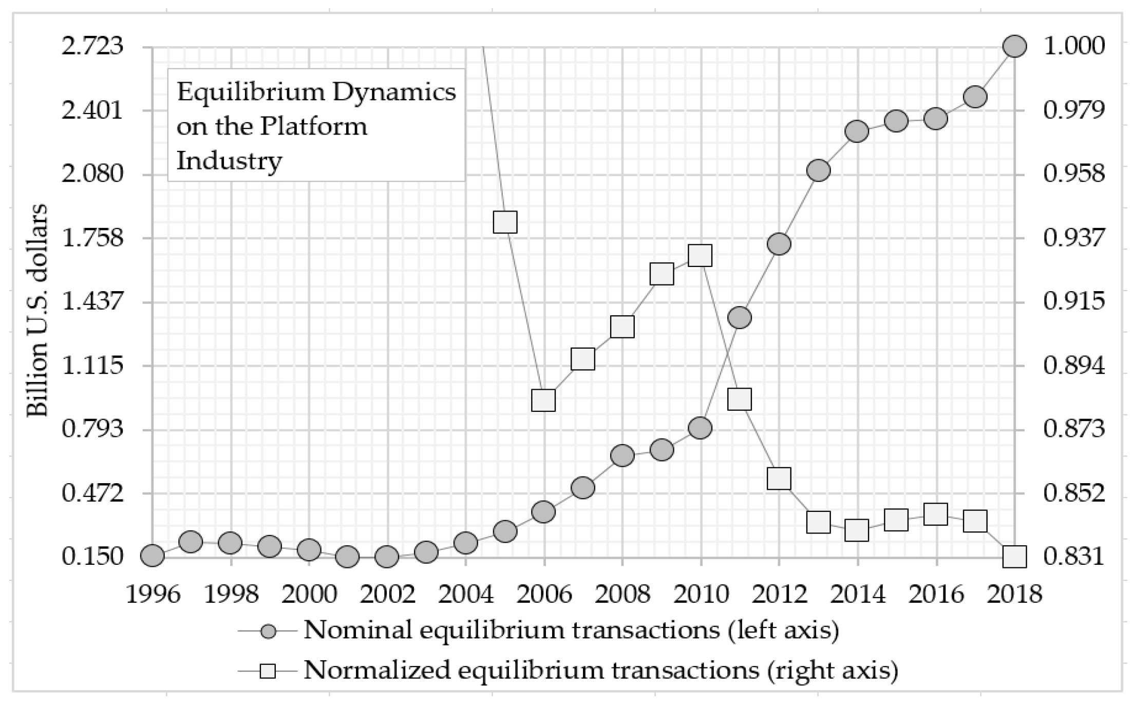
As a result, the equilibrium transaction behavior of the produce/selling and the purchase/buying agents of the platform industry was completely detected by the above computational model and distributed into the following time phases (see Figure 3, the histogram with round marker with gray fill and the histogram with square marker with white fill, Table 6, column (a)-(b)):
- -
- The first time phases cover the period from 1995 to 2004. This period is distinguished by the fact that it does not belong to the feasible domain of solutions for the equilibrium transactions of platform industry produce/selling and purchase/buying agents. That is, for first-time phases the financial and insurance industry has an entry point of 0.159, a peak deviation of 0.228, and an exit point of 0.221 billion U.S. dollars;
- -
- The initial median average was 0.198 and the final median average of the first time phases was 0.174 billion U.S. dollars. That is, in the first time phases, the median average absolute value of equilibrium transactions in the financial and insurance sector decreased by 0.025 billion U.S. dollars, and the median average relative value of equilibrium transactions decreased by 87.52%;
- -
- The second time phases cover the period from 2005 to 2018, this period is in the feasible domain of solution of equilibrium transactions of produce/selling and purchase/buying agents of the platform industry. That is, for the second time phases the financial and insurance industry has an entry point of 0.279, a peak deviation of 2.470, and an exit point of 2.723 billion U.S. dollars;
Figure 3.
Nominal and normalized equilibrium dynamics of the platform produce/selling and purchase/buying transactions in the financial and insurance activities industry.
Figure 3.
Nominal and normalized equilibrium dynamics of the platform produce/selling and purchase/buying transactions in the financial and insurance activities industry.
- -
- The initial median average was 0.666 and the final median average for the second time phase was 2.288 billion U.S. dollars. That is, in the second time phase, the median average absolute value of equilibrium transactions in the financial and insurance sector increased by 1.622 billion U.S. dollars, and the median average relative value of equilibrium transactions increased by 343.36%.
Thus, analyzing the entry points, peak deviations, exit points, time phases, and increase or decrease of median average values of these transactions enables a deeper insight into the fundamental patterns of inter-industry linkages, which help address theoretical and practical issues related to platform agent’s behavior.
As a result, in Section 3.1 we created, substantiated, and implemented of the computational model on the determine equilibrium states by aligning supply and demand functions of the produce/selling and purchase/buying transactions. The novelty of these results are definition of equilibrium transactions; analysis of time phases of undervalued and overvalued transactions; classification of time phases of equilibrium growth within the area of admissible solutions of the produce/selling and purchase/buying and the significance may be to use resources efficiently and ensure sustainable growth in the financial and insurance activities of Kazakhstan.
Table 6.
Dynamics of nominal and normalized equilibrium transactions of the platform industry and its internal and external ecosystem for Kazakhstan’s financial and insurance activities.
Table 6.
Dynamics of nominal and normalized equilibrium transactions of the platform industry and its internal and external ecosystem for Kazakhstan’s financial and insurance activities.
| Year | (a) | (b) | (c) | (d) | (e) | (f) | Year | (a) | (b) | (c) | (d) | (e) | (f) |
|---|---|---|---|---|---|---|---|---|---|---|---|---|---|
| NaN | NaN | NaN | NaN | NaN | NaN | 0.501 | 0.896 | 0.861 | 0.233 | 0.146 | 0.921 | ||
| 0.159 | 5.209 | 0.681 | –1.279 | 0.019 | 4.433 | 0.658 | 0.907 | 1.012 | 0.215 | 0.314 | 0.877 | ||
| 0.228 | 4.191 | 0.645 | –0.670 | 0.023 | 1.295 | 0.689 | 0.925 | 1.096 | 0.195 | 0.359 | 0.875 | ||
| 0.220 | 3.773 | 0.677 | –0.515 | 0.024 | 1.351 | 0.802 | 0.931 | 1.164 | 0.173 | 0.360 | 0.884 | ||
| 0.200 | 3.260 | 0.570 | –0.047 | 0.026 | 1.366 | 1.358 | 0.883 | 1.185 | 0.160 | 0.362 | 0.891 | ||
| 0.186 | 2.470 | 0.568 | –0.047 | 0.026 | 1.063 | 1.728 | 0.857 | 1.236 | 0.151 | 0.373 | 0.893 | ||
| 0.150 | 1.759 | 0.564 | –0.104 | 0.027 | 1.061 | 2.097 | 0.842 | 1.340 | 0.144 | 0.369 | 0.898 | ||
| 0.151 | 1.454 | 0.561 | –0.119 | 0.029 | 1.032 | 2.296 | 0.840 | 1.427 | 0.136 | 0.377 | 0.893 | ||
| 0.173 | 1.244 | 0.551 | 0.035 | 0.033 | 1.041 | 2.348 | 0.843 | 1.583 | 0.141 | 0.392 | 0.883 | ||
| 0.221 | 1.043 | 0.596 | 0.219 | 0.041 | 1.034 | 2.356 | 0.845 | 1.699 | 0.148 | 0.393 | 0.889 | ||
| 0.279 | 0.942 | 0.705 | 0.279 | 0.042 | 0.996 | 2.470 | 0.843 | 1.784 | 0.147 | 0.395 | 0.890 | ||
| 0.378 | 0.883 | 0.766 | 0.258 | 0.051 | 0.936 | 2.723 | 0.831 | 1.783 | 0.137 | 0.400 | 0.888 |
Note. (a) Nominal equilibrium transactions of the platform industry. (b) Normalized equilibrium transactions of the platform industry. (c) Nominal equilibrium transactions of the internal ecosystem. (d) Normalized equilibrium transactions of the internal ecosystem. (e) Nominal equilibrium transactions of the external ecosystem. (f) Normalized equilibrium transactions of the external ecosystem. A Billion U.S. dollars. Compiled by the authors.
3.2. An Algorithm for Determine the Equilibrium of the Internal Ecosystem and Its Application
In Section 3.2 we focus on developing and applying computational model to detect equilibrium transactions within the internal ecosystem of Kazakhstan's financial and insurance activities industry. The usage of normalized data, regression equations, iterative techniques, operations research, mathematical programming and computational model to detect equilibrium transactions allows us to get information on the equilibrium state of internal ecosystem flows and their role in achieving equilibrium growth.
3.2.1. Creating an Algorithm to Determine the Equilibrium in the Internal Ecosystem
Entry: – the internal ecosystem payment transactions of the total input of financial and insurance activities industry, , , a billion U.S. dollars (see Table 1, column (c)); – the internal ecosystem final demand transactions of the total output of the financial and insurance activities industry, , , a billion U.S. dollars (see Table 1, column (d)).
Outcome: Equilibrium transactions of the internal ecosystem payment and final demand, respectively, of the total input and the total output of financial and insurance activities industry.
Step 1: To create the supply function as a data set on the normalized internal ecosystem payment transactions [0;1] from the domain of the observation , , .
(i) Sorting by the growth of data , , , i.e. rearrange the elements of observation data , , , into a sequence such that the following chains of inequalities hold: , and denote by , (see Table 3, column (c)), where
and
(ii) Calculate the cumulative sum of sorted data , :
(iii) To normal the cumulative sum of sorted data , :
and denote by , (see Table 4, column (c));
(iv) To build and to visualize the supply as a function of normalized internal ecosystem payment transactions from the domain of the observation , (see Figure 4, histogram with a round marker with a gray fill);
Step 2: Create the regression equations for the supply function of the internal ecosystem payment transactions , .
(i) Calculate the slope between the dependent and the independent variable , ;
(ii) Calculate the intercept between the dependent and the independent variable , ;
(iii) Calculate the R–square for the regression equation between the dependent and the independent variable , ;
(iv) Calculate the p–value of parameters for the regression equation between the dependent and the independent variable , ;
(v) Calculate the standard errors of parameters for the regression equation between the dependent and the independent variable , ;
Table 7.
Results of the intelligent analysis of equilibrium growth in the internal ecosystem.
| Year | (a) | (b) | (c) | (d) | (e) | (f) | Year | (a) | (b) | (c) | (d) | (e) | (f) |
|---|---|---|---|---|---|---|---|---|---|---|---|---|---|
| 0.803 | –0.198 | UV | 1.874 | –0.121 | UV | 2.469 | 1.360 | OV | 0.721 | 0.141 | OV | ||
| 0.867 | –0.218 | UV | 1.735 | –0.009 | UV | 2.850 | 1.005 | OV | 0.657 | 0.140 | OV | ||
| 0.940 | –0.199 | UV | 1.599 | 0.102 | UV | 3.272 | 0.996 | OV | 0.602 | 0.077 | OV | ||
| 1.015 | –0.257 | UV | 1.488 | –0.106 | UV | 3.708 | 0.710 | OV | 0.562 | –0.056 | UV | ||
| 1.093 | –0.307 | UV | 1.378 | –0.019 | UV | 4.192 | 0.709 | OV | 0.522 | –0.032 | UV | ||
| 1.170 | –0.382 | UV | 1.287 | –0.153 | UV | 4.678 | 0.232 | OV | 0.486 | –0.040 | UV | ||
| 1.249 | –0.450 | UV | 1.198 | –0.088 | OV | 5.210 | 0.180 | OV | 0.452 | –0.026 | UV | ||
| 1.336 | –0.462 | UV | 1.110 | –0.021 | OV | 5.804 | 0.209 | OV | 0.420 | –0.015 | UV | ||
| 1.445 | –0.344 | UV | 1.024 | 0.045 | OV | 6.406 | –0.315 | UV | 0.392 | –0.054 | UV | ||
| 1.598 | –0.042 | UV | 0.939 | 0.117 | OV | 7.048 | –0.554 | UV | 0.365 | –0.030 | UV | ||
| 1.802 | 0.258 | OV | 0.864 | 0.072 | OV | 7.695 | –1.141 | UV | 0.340 | –0.023 | UV | ||
| 2.091 | 0.836 | OV | 0.790 | 0.131 | OV | 8.361 | –1.623 | UV | 0.317 | –0.032 | UV |
Note. (a) Supply function values for the payment transactions. (b) Nominal estimate of the equilibrium of the payment transactions. (c) Linguistic variables: Undervalue and Overvalue of the equilibrium of the payment transactions. (d) Demand function values for the final demand transactions. (e) Nominal estimate of the equilibrium the final demand transactions. (f) Linguistic variables: Undervalue and Overvalue of the equilibrium of the final demand transactions. A Billion U.S. dollars. Compiled by the authors.
(vi) To build the regression equations for the supply function of the normalized data of the internal ecosystem payment transactions on the domain of the observation data , [30]:
where unknown parameters Slope’, Intercept’, R–square, p–value, and Standard errors will be estimated by the least squares in the above sub steps (i)–(v);
(vii) Visualize the regression equations for the supply function of the normalized data of the internal ecosystem payment transactions on the domain of the observation data , (see Figure 4, a dotted line with one dot, Table 7, column (a)).
Step 3: Create the demand function for the normalized data set of the internal ecosystem final demand transactions on the domain of the observation data set , .
(i) Descending sorted of data , , i.e. rearrange the elements of observation data , into a sequence such that the following chains of inequalities hold: , and denote by , (see Table 3, column (d)), where
and
(ii) Calculate the cumulative sum of sorted data , :
(iii) To normal the cumulative sum of sorted data , :
and denote by , ;
(iv) To build and visualize the demand function to normalized platform final demand transactions from the domain of the observation , (see Figure 4, histogram with a square marker with a white fill);
Step 4: Create the regression equations for the demand function of the internal ecosystem final demand transactions: , .
(i) Calculate the slope between the dependent and the independent variable , ;
(ii) Calculate the intercept between the dependent and the independent variable , ;
(iii) Calculate the R–square for the regression equation between the dependent and the independent variable , ;
(iv) Calculate the p–value of parameters for the regression equation between the dependent and the independent variable , ;
(v) Calculate the standard errors of parameters for the regression equation between the dependent and the independent variable , ;
(vi) To build the regression equations for the demand function of the platform purchase/buying transactions , [35]:
where unknown parameters Slope, Intercept, R–square, p–value, Standard errors will be estimated by the least squares in the above sub-steps (i)–(v);
(vii) Visualize the regression equations for the demand function of the internal ecosystem final demand transactions , (see Figure 4, the dotted line with two dots, Table 7, column (d)).
Step 5: Find the equilibrium transactions of the internal ecosystem payment for the financial and insurance activities industry, i.e. prove that .
(i) Construct equations for the equilibrium transactions of the internal ecosystem payment and the final demand from the equality condition of equations (14) and (15), i.e. . Indeed, from (14) and (15) we obtain:
(ii) Find the normalized sequences , , such that these functions satisfied conditions (16):
(iia) If for , , the following holds:
then we use linear interpolation and ensure convergence of the iteration using the gradient method [31]:
(iib) If for , , the following holds:
or
Then, respectively, we use linear extrapolation and ensure convergence of the iteration by the gradient method [31]:
or
Step 6: Find the equilibrium transactions of the internal ecosystem final demand for the financial and insurance activities industry, i.e. prove that .
(i) Construct equations for the equilibrium transactions of the internal ecosystem final demand and the internal ecosystem payment from the equality condition of equations (14) and (15), i.e. . Indeed, from (14) and (15) we obtain:
(ii) Find the normalized sequences , , such that these functions satisfied conditions (20):
(iia) If for , , the following holds:
then we use linear interpolation and ensure convergence of the iteration using the gradient method [31]:
(iib) If for , , the following holds:
or
Then, respectively, we use linear extrapolation and ensure convergence of the iteration by the gradient method [31]:
or
3.2.2. Simulation and Its Application in Intelligent Analysis of Equilibrium Growth of the Internal Ecosystem
In Section 3.2, the behavior of internal ecosystem payment transactions is evaluated using the supply function, while the behavior of internal ecosystem final demand transactions is evaluated using the demand function.
First, the regression equation (14) is created for internal ecosystem payment agent behavior, where the dependent variable is normalized payment, and the independent variable is observed payment transactions.
The regression equation, using the Slope' and Intercept' parameters and the normalized payment transaction dependent variable values estimated through the least squares, provides the estimated supply function values:
Also, the values obtained by subtracting the observed payment transactions from the calculated payment transactions represent the estimates of the internal ecosystem payment behavior.
Thus, we use computational model to detect the equilibrium to identify time phases of undervalued and overvalued nominal estimate and linguistic variables in the internal ecosystem payment of the financial and insurance activities industry we get (see Table 7, column (b)-(c)):
- -
- The first phase of undervalued the internal ecosystem payment of the financial and insurance activities industry is characterized by a flow of transactions with the following attributes: an entry point of 0.198, a peak deviation of 0.462, and an exit point of 0.042 billion U.S. dollars in undervalued transactions;
- -
- The phase of overvalued internal ecosystem payment of the financial and insurance activities industry is characterized by a flow of transactions with the following attributes: an entry point of 0.258, a peak deviation of 1.360, and an exit point of 0.209 billion U.S. dollars in overvalued transactions;
- -
- The second phase of undervalued the internal ecosystem payment of the financial and insurance activities industry is characterized by a flow of transactions with the following attributes: an entry point of 0.315, a peak deviation of 1.141, and an exit point of 1.623 billion U.S. dollars in undervalued transactions.
Next, for the internal ecosystem final demand behavior, a regression equation (15) is created, where the dependent variable is the normalized final demand transactions and the independent variable is the observed final demand transactions. Using Slope, Intercept parameters, values of normalized final demand transaction dependent variable and least squares were estimated the parameters of the regression equation and the demand function values are calculated:
Also, the values obtained by subtracting the observed final demand transactions from the calculated final demand transactions represent the estimates of the internal ecosystem's final demand behavior.
We now apply computational model to establish equilibrium, determine time phases of undervaluation and overvaluation of nominal estimate and linguistic variables within the internal ecosystem final demand in the financial and insurance activities industry we get (see Table 7, column (e)-(f)):
- -
- The first phase of undervalued of the internal ecosystem final demand of the financial and insurance activities industry is characterized by a flow of transactions with the following attributes: an entry point of 0.121, a peak deviation of 0.106, and an exit point of 0.021 billion U.S. dollars in undervalued transactions;
- -
- The phase of overvalued of the internal ecosystem final demand of the financial and insurance activities industry is characterized by a flow of transactions with the following attributes: an entry point of 0.045, a peak deviation of 0.141, and an exit point of 0.077 billion U.S. dollars in overvalued transactions;
- -
- The second phase of undervalued of the internal ecosystem final demand of the financial and insurance activities industry is characterized by a flow of transactions with the following attributes: an entry point of 0.056, a peak deviation of 0.054, and an exit point of 0.032 billion U.S. dollars in undervalued transactions.
Also, in Section 3.2, based on studies of the behavior of payment and final demand agents, work is carried out to detect the equilibrium points of the stochastic dynamic state of the internal ecosystem. Indeed, regression equations (14) and (15) are constructed respectively by applying the least squares method to the supply function of the payment transactions data and the demand function of the final demand transactions. This, in turn, the problem of determining the equilibrium points in the behavior of the mentioned payment and final demand agents leads to the problem of calculating the intersection points of the linear equations (14) of supply and (15) of demand function.
First, for an internal ecosystem payment agent, if the equilibrium point lies in the feasible domain of solution, then the desired point is detected using the linear interpolation and the gradient method defined by equation (17). The stopping criterion for iterative calculations is obtained from equality (16). Also for the internal ecosystem payment, if the equilibrium point does not belong to the feasible domain of solution, then the desired point is detected by equation (18) for the left side and equation (19) for the right side and It is determining by linear extrapolation and gradient method. The stopping criterion for iterative calculations is obtained from equality (16).
Second, for a final demand of an internal ecosystem, if the equilibrium point lies in the feasible domain of solution, then the desired point is detected by linear interpolation and gradient method, defined by equation (21). The criterion for stopping the iterative calculations is obtained from equality (20). Also for the final demand of the internal ecosystem, if the equilibrium point does not belong to the feasible domain of solution, then the desired point is detected by equation (22) for the left part, and (23) for the right part, and It is determining by linear extrapolation and gradient method. The criterion for stopping the iterative calculations is obtained from equilibrium (20).
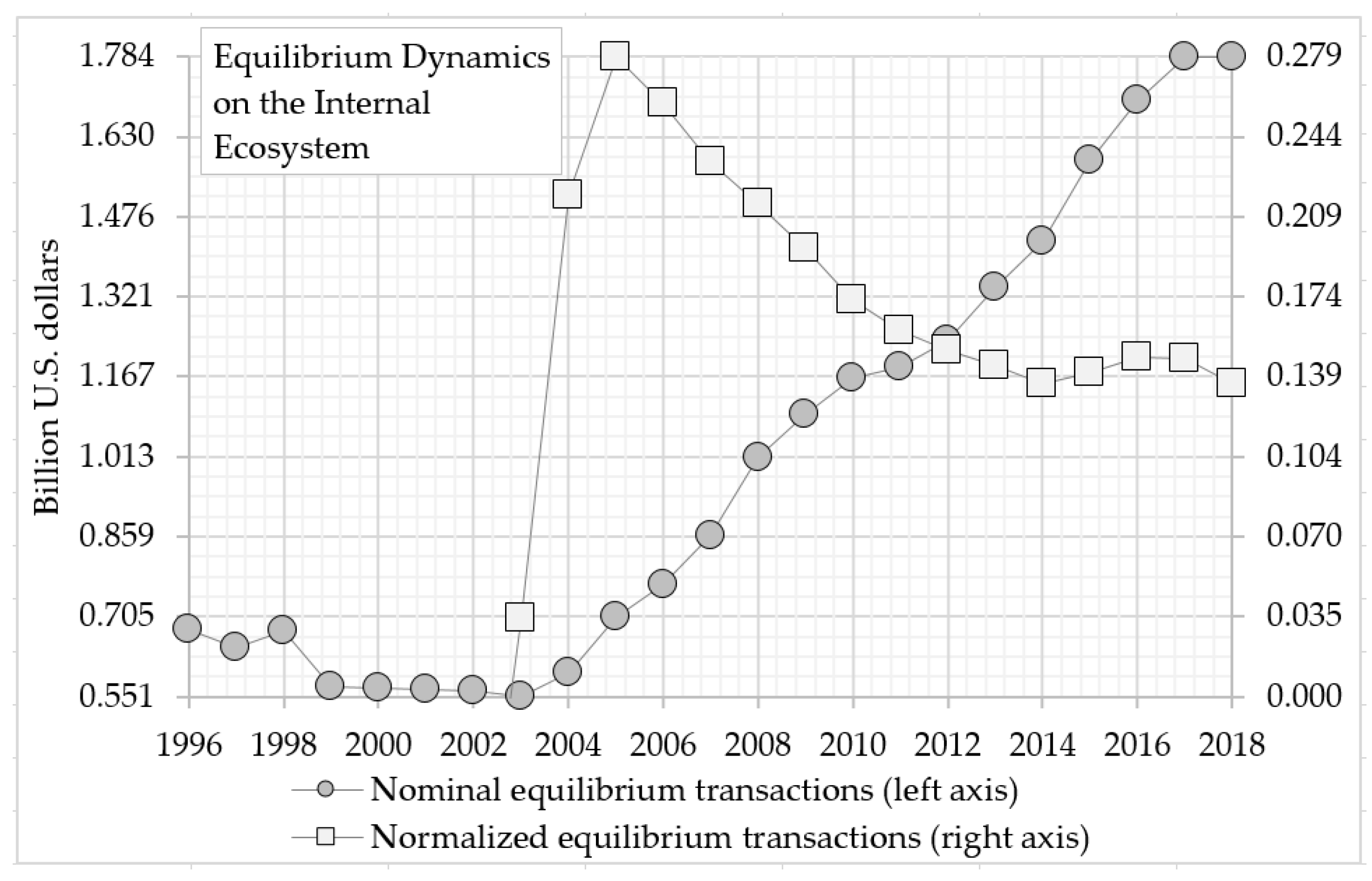
As a result, the equilibrium transaction behavior of the payment and the final demand agents of the internal ecosystem was completely defined and distributed into the following time phases (see Figure 5, the histogram with round marker with gray fill and the histogram with a square marker with white fill, Table 6, column (c)-(d)):
- -
- The first time phases cover the period from 1995 to 2002. This period is distinguished by the fact that it does not belong to the feasible domain of solution for the equilibrium transactions of internal ecosystem payment and final demand agents. That is, for first-time phases the financial and insurance industry has an entry point of 0.681, a peak deviation of 0.677, and an exit point of 0.570 billion U.S. dollars;
- -
- The initial median average was 0.643 and the final median average of the first time phases was 0.565 billion U.S. dollars. That is, in the first time phases, the median average absolute value of equilibrium transactions in the financial and insurance sector decreased by 0.079 billion U.S. dollars, and the median average relative value of equilibrium transactions decreased by 87.74%;
- -
- The second time phases cover the period from 2003 to 2018, this period is in the feasible domain of solution of equilibrium transactions of payment and the final demand agents of the internal ecosystem. That is, for the second time phases the financial and insurance industry has an entry point of 0.551, a peak deviation of 1.096, and an exit point of 1.164 billion U.S. dollars;
- -
- The initial median average was 0.844 and the final median average for the second time phase was 1.505 billion U.S. dollars. That is, in the second time phase, the median average absolute value of equilibrium transactions in the financial and insurance sector increased by 0.661 billion U.S. dollars, and the median average relative value of equilibrium transactions increased by 178.31%.
Figure 5.
Nominal and normalized equilibrium dynamics of the internal ecosystem payment and final demand transactions in the financial and insurance activities industry.
Figure 5.
Nominal and normalized equilibrium dynamics of the internal ecosystem payment and final demand transactions in the financial and insurance activities industry.
Thus, analyzing the entry points, peak deviations, exit points, time phases, and increase or decrease of median average values of these transactions enables a deeper insight into the fundamental patterns of inter-industry linkages, which help address theoretical and practical issues related to the internal ecosystem agent’s behavior.
In Section 3.2 we created, substantiated, and implemented of the computational model on the determine equilibrium states by aligning supply and demand functions of the internal ecosystem transactions. The novelty of these results are definition of equilibrium transactions; analysis of time phases of undervalued and overvalued transactions; classification of time phases of equilibrium growth within the area of admissible solutions of the internal ecosystem payments and demand, classifying equilibrium transactions and the significance may be to use resources efficiently and ensure sustainable growth in the financial and insurance activities of Kazakhstan.
3.3. An Algorithm for Determine the Equilibrium on the External Ecosystem and Its Application
In Section 3.3 we offer on the development and application of computational model to detect equilibrium transactions within the external ecosystem of Kazakhstan's financial and insurance activities industry. By analyzing import (outflow and (or) demand for foreign currency) and export (inflow and (or) supply for foreign currency) transactions, the algorithm employs normalized data, regression modeling, operations research and mathematical programming to align supply and demand functions, providing a systematic approach to understanding external ecosystem interactions and achieving equilibrium growth.
3.3.1. An Algorithm for Determine the Equilibrium on the External Ecosystem
Entry: Let – the external ecosystem export (inflow and (or) supply for foreign currency) transactions of the total output of financial and insurance activities industry, , , a billion U.S. dollars (see Table 1, column (f)); – the external ecosystem import (outflow and (or) demand for foreign currency) transactions of the total input of financial and insurance activities industry, , , a billion U.S. dollars (see Table 1, column (e)).
Outcome: Equilibrium transactions of the external ecosystem import and exports, respectively, of the total input and the total output of the financial and insurance activities industry.
Step 1: To create the supply function as a data set on the normalized external ecosystem export transactions [0;1] from the domain of the observation , .
(i) Sorting by growth of data , , i.e. rearrange the elements of observation data , into a sequence such that the following chains of inequalities hold: , and denote by , (see Table 3, column (f)), where
and
(ii) Calculate the cumulative sum of sorted data , :
(iii) To normal the cumulative sum of sorted data , :
and denote by , (see Table 4, column (f));
(iv) To build and to visualize the supply as function to normalized of external ecosystem export transactions from domain of the observation ,
(see Figure 6, histogram with a round marker with a gray fill);
Step 2: Create the regression equations for the supply function of the external ecosystem export transactions , .
(i) Calculate the slope between the dependent and the independent variable , ;
(ii) Calculate the intercept between the dependent and the independent variable , ;
(iii) Calculate the R–square for the regression equation between the dependent and the independent variable , ;
(iv) Calculate the p–value of parameters for the regression equation between the dependent and the independent variable , ;
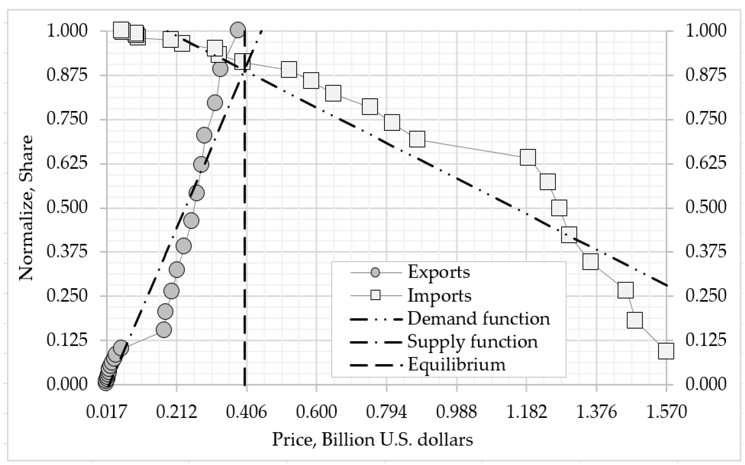
Figure 6.
Observation, regression equations, and equilibrium of the external ecosystem import and export transactions in the financial and insurance activities industry.
Figure 6.
Observation, regression equations, and equilibrium of the external ecosystem import and export transactions in the financial and insurance activities industry.
(v) Calculate the standard errors of parameters for the regression equation between the dependent and the independent variable , ;
(vi) To build the regression equations for the supply function of the normalized data of the internal ecosystem payment transactions on domain of the observation data , [30]:
where unknown parameters Slope’, Intercept’, R–square, p–value, and Standard errors will be estimated by the least squares in the above sub steps (i)–(v);
(vii) Visualize the regression equations for the supply function of the normalized data of the external ecosystem export transactions on the domain of the observation data , (see Figure 6, a dotted line with one dot, Table 8, column (a)).
Table 8.
Results of the intelligent analysis of equilibrium growth in the external ecosystem.
| Year | (a) | (b) | (c) | (d) | (e) | (f) | Year | (a) | (b) | (c) | (d) | (e) | (f) |
|---|---|---|---|---|---|---|---|---|---|---|---|---|---|
| 0.026 | –0.009 | UV | 1.933 | –0.363 | UV | 0.089 | 0.089 | OV | 0.460 | 0.126 | OV | ||
| 0.029 | –0.011 | UV | 1.765 | –0.281 | UV | 0.111 | 0.070 | OV | 0.400 | 0.125 | OV | ||
| 0.031 | –0.010 | UV | 1.599 | –0.141 | UV | 0.135 | 0.065 | OV | 0.355 | 0.040 | OV | ||
| 0.034 | –0.012 | UV | 1.445 | –0.084 | UV | 0.161 | 0.052 | OV | 0.318 | 0.013 | OV | ||
| 0.036 | –0.014 | UV | 1.297 | 0.004 | OV | 0.189 | 0.044 | OV | 0.282 | 0.038 | OV | ||
| 0.040 | –0.014 | UV | 1.153 | 0.122 | OV | 0.220 | 0.033 | OV | 0.256 | –0.027 | UV | ||
| 0.043 | –0.016 | UV | 1.012 | 0.230 | OV | 0.252 | 0.016 | OV | 0.233 | –0.036 | UV | ||
| 0.046 | –0.017 | UV | 0.877 | 0.311 | OV | 0.286 | –0.006 | UV | 0.221 | –0.116 | UV | ||
| 0.050 | –0.017 | UV | 0.777 | 0.105 | OV | 0.322 | –0.032 | UV | 0.210 | –0.108 | UV | ||
| 0.055 | –0.016 | UV | 0.685 | 0.125 | OV | 0.360 | –0.040 | UV | 0.198 | –0.099 | UV | ||
| 0.060 | –0.017 | UV | 0.600 | 0.149 | OV | 0.401 | –0.067 | UV | 0.191 | –0.127 | UV | ||
| 0.068 | –0.007 | UV | 0.526 | 0.120 | OV | 0.447 | –0.064 | UV | 0.184 | –0.126 | UV |
Note. (a) Supply function values for the export transactions. (b) Nominal estimate of the equilibrium, of the export transactions. (c) Linguistic variables: Undervalue and Overvalue of the equilibrium of the export transactions. (d) Demand function values for the import transactions. (e) Nominal estimate of the equilibrium of the import transactions. (f) Linguistic variables: Undervalue and Overvalue of the equilibrium the import transactions. A Billion U.S. dollars. Compiled by the authors.
Step 3: To create the demand function as a data set on the normalized of the external ecosystem import transactions [0;1] from the domain of the observation , .
(i) Descending sorted of data , , i.e. rearrange the elements of observation data , into a sequence such that the following chains of inequalities hold: , and denote by , (see Table 3, column (e)), where
and
(ii) Calculate the cumulative sum of sorted data , :
(iii) To normal the cumulative sum of sorted data , :
and denote by , ;
(iv) To build and visualize the demand function to normalized external ecosystem import transactions from the domain of the observation, (see Figure 6, histogram with a square marker with a white fill);
Step 4: Create the regression equations for the demand function of the external ecosystem import transactions: , .
(i) Calculate the slope between the dependent and the independent variable , ;
(ii) Calculate the intercept between the dependent and the independent variable , ;
(iii) Calculate the R–square for the regression equation between the dependent and the independent variable , ;
(iv) Calculate the p–value of parameters for the regression equation between the dependent and the independent variable , ;
(v) Calculate the standard errors of parameters for the regression equation between the dependent and the independent variable , ;
(vi) To build the regression equations for the demand function of the external ecosystem import transactions , [35]:
where unknown parameters Slope, Intercept, R–square, p–value, and Standard errors will be estimated by the least squares in the above sub-steps (i)–(v);
(vii) Visualize the regression equations for the demand function of the external ecosystem import transactions , (see Figure 6, the dotted line with two dots, Table 8, column (d)).
Step 5: Find the equilibrium transactions of the external ecosystem export for the financial and insurance activities industry, i.e. prove that .
(i) Construct equations for the equilibrium transactions of the external ecosystem the exports and import from the equality condition of equations (24) and (25), i.e. . Indeed, from (24) and (25) we obtain:
(ii) Find the normalized sequences , , such that these functions satisfied conditions (26):
(iia) If for , , the following holds:
then we use linear interpolation and ensure convergence of the iteration using the gradient method [31]:
(iib) If for , , the following holds:
or
Then, respectively, we use linear extrapolation and ensure convergence of the iteration by the gradient method [31]:
or
Step 6: Find the equilibrium transactions of the external ecosystem imports for the financial and insurance activities industry, i.e. prove that
.
(i) Construct equations for the equilibrium transactions of the external ecosystem exports and the external ecosystem import from the equality condition of equations (24) and (25), i.e. . Indeed, from (24) and (25) we obtain:
(ii) Find the normalized sequences , , such that these functions satisfied conditions (30):
(iia) If for , , the following holds:
then we use linear interpolation and ensure convergence of the iteration using the gradient method [36]:
(iib) If for , , the following holds:
or
Then, respectively, we use linear extrapolation and ensure convergence of the iteration by the gradient method [36]:
or
3.3.2. Simulation and Its Application in Intelligent Analysis of Equilibrium Growth of the External Ecosystem
In Section 3.3, the behavior of external ecosystem export (inflow and (or) supply for foreign currency) transactions is evaluated using the supply function, while the behavior of external ecosystem imports (outflow and (or) demand for foreign currency) transactions is evaluated using the demand function.
First, the regression equation (24) is created for external ecosystem export agent behavior, where the dependent variable is normalized export transactions, and the independent variable is observed export transactions.
The regression equation, using the Slope’ and Intercept’ parameters and the normalized external ecosystem exports transaction dependent variable values estimated through the least squares, provides the estimated supply function values:
Also, the values obtained by subtracting the observed export transactions from the calculated export transactions represent the estimates of the external ecosystem export behavior.
Thus, we use computational model to detect the equilibrium to identify time phases of undervalued and overvalued nominal estimate and linguistic variables in the external ecosystem export of the financial and insurance activities industry we get (see Table 8, column (b)-(c)):
- -
- The first phase of undervalued the external ecosystem export of the financial and insurance activities industry is characterized by a flow of transactions with the following attributes: an entry point of 0.009, a peak deviation of 0.017, and an exit point of 0.007 billion U.S. dollars in undervalued transactions;
- -
- The phase of overvalued external ecosystem export of the financial and insurance activities industry is characterized by a flow of transactions with the following attributes: an entry point of 0.089, a peak deviation of 0.070, and an exit point of 0.016 billion U.S. dollars in overvalued transactions;
- -
- The second phase of undervalued the external ecosystem export of the financial and insurance activities industry is characterized by a flow of transactions with the following attributes: an entry point of 0.006, a peak deviation of 0.067, and an exit point of 0.064 billion U.S. dollars in undervalued transactions.
Next, for the external ecosystem import behavior, a regression equation (25) is created, where the dependent variable is the normalized export transactions and the independent variable is the observed import transactions. Using Slope, Intercept parameters, values of normalized import transaction dependent variable, and least squares were estimated the parameters of the regression equation and the demand function values are calculated:
Also, the values obtained by subtracting the observed import transactions from the calculated import transactions represent the estimates of the external ecosystem import behavior.
We now apply computational model to establish equilibrium, determine time phases of undervaluation and overvaluation of nominal estimate and linguistic variables within the external ecosystem import in the financial and insurance activities industry (see Table 8, column (e)-(f)):
- -
- The first phase of undervalued of the external ecosystem import of the financial and insurance activities industry is characterized by a flow of transactions with the following attributes: an entry point of 0.363, a peak deviation of 0.281, and an exit point of 0.084 billion U.S. dollars in undervalued transactions;
- -
- The phase of overvalued external ecosystem import of the financial and insurance activities industry is characterized by a flow of transactions with the following attributes: an entry point of 0.004, a peak deviation of 0.149, and an exit point of 0.038 billion U.S. dollars in overvalued transactions;
- -
- The second phase of undervalued the external ecosystem import of the financial and insurance activities industry is characterized by a flow of transactions with the following attributes: an entry point of 0.027, a peak deviation of 0.127, and an exit point of 0.126 billion U.S. dollars in undervalued transactions.
Also, in Section 3.3, based on studies of the behavior of import and export agents, work is carried out to detect the equilibrium points of the stochastic dynamic state of the external ecosystem. Indeed, regression equations (24) and (25) are constructed respectively by applying the least squares method to the supply function of the import transactions data and the demand function of the export transactions. This, in turn, the problem of determining the equilibrium points in the behavior of the mentioned import and export agents leads to the problem of calculating the intersection points of the linear equations (24) of supply and (25) of demand function.
First, for the external ecosystem import agent, if the equilibrium point lies in the feasible domain of the solution, then the desired point is detected using the linear interpolation and the gradient method defined by equation (27). The stopping criterion for iterative calculations is obtained from equality (26). Also for the import of the external ecosystem, if the equilibrium point does not belong to the feasible domain of solution, then the desired point is detected by equation (28) for the left side, and equation (29) for the right side and It is determining by linear extrapolation and gradient method. The stopping criterion for iterative calculations is obtained from equality (26).
Second, for an export of an external ecosystem, if the equilibrium point lies in the feasible domain of solution, then the desired point is detected by linear interpolation and gradient method, defined by equation (31). The criterion for stopping the iterative calculations is obtained from equality (30). Also, for the export of the external ecosystem, if the equilibrium point does not belong to the feasible domain of solution, then the desired point is detected by equation (32) for the left part and (33) for the right part, and It is determining by linear extrapolation and gradient method. The criterion for stopping the iterative calculations is obtained from equilibrium (30).
As a result, the equilibrium transaction behavior of the export and the import agents of the external ecosystem industry was completely determining by the above model and distributed into the following time phases (see Figure 7, the histogram with round marker with gray fill and the histogram with square marker with white fill, Table 6, column (e)-(f)):
- -
- The first time phases cover the period from 1995 to 2004. This period is distinguished by the fact that it does not belong to the feasible domain of solution for the equilibrium transactions of external ecosystem import and export agents. That is, for first time phases the financial and insurance industry has an entry point of 0.019, a peak deviation of 0.033, and an exit point of 0.041 billion U.S. dollars;
Figure 7.
Nominal and normalized equilibrium dynamics of the external ecosystem import and export transactions in the financial and insurance activities industry.
Figure 7.
Nominal and normalized equilibrium dynamics of the external ecosystem import and export transactions in the financial and insurance activities industry.
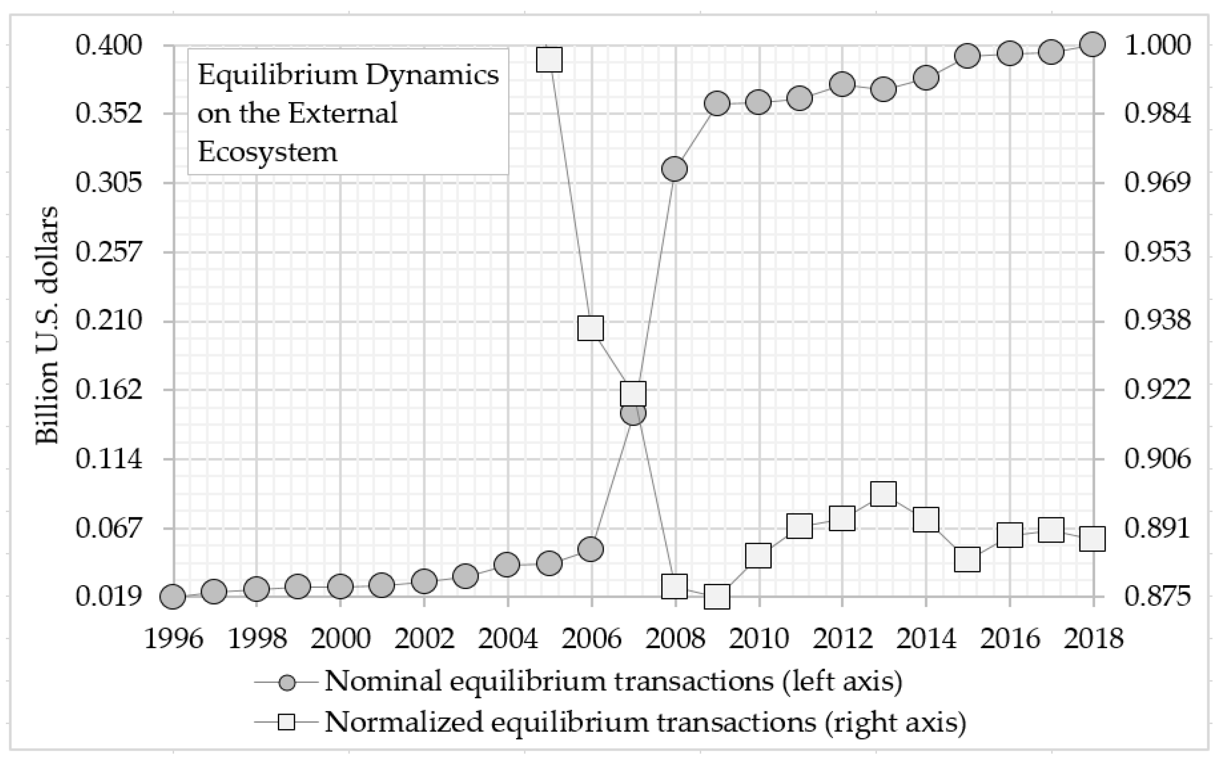
- -
- The initial median average was 0.024 and the final median average of the first-time phases was 0.033 billion U.S. dollars. That is, in the first time phase, the median average absolute value of equilibrium transactions in the financial and insurance sector increased by 0.009 billion U.S. dollars, and the median average relative value of equilibrium transactions decreased by 138.41%;
- -
- The second time phases cover the period from 2005 to 2018, this period is in the feasible domain of solution of equilibrium transactions of import and export agents of the external ecosystem. That is, for the second time phase the financial and insurance industry has an entry point of 0.042, a peak deviation of 0.395, and an exit point of 0.400 billion U.S. dollars;
- -
- The initial median average was 0.234 and the final median average for the second time phase was 0.386 billion U.S. dollars. That is, in the second time phase, the median average absolute value of equilibrium transactions in the financial and insurance sector increased by 0.152 billion U.S. dollars, and the median average relative value of equilibrium transactions increased by 165.07%.
Thus, analyzing the entry points, peak deviations, exit points, time phases, and increase or decrease of median average values of these transactions enables a deeper insight into the fundamental patterns of inter-industry linkages, which help address theoretical and practical issues related to external ecosystem agent’s behavior.
Based on the results of Section 3.3, we created substantiated and implemented of the computational model on the determine equilibrium states for external ecosystem transactions by alignment import (outflow and (or) demand for foreign currency) and export (inflow and (or) supply for foreign currency) flows. The novelty of these results are determine equilibrium transactions; analysis of time phases of undervalued and overvalued transactions; classification of time phases of equilibrium growth within the area of admissible solutions of the external ecosystem imports and exports, classifying equilibrium transactions and the significance may be to use resources efficiently and ensure sustainable growth in the financial and insurance activities of Kazakhstan.
4. Discussion
The application of computational model to the investigation of equilibrium growth in Kazakhstan's insurance and financial sectors presents important opportunities and serious challenges. The diverse lessons that recent studies of platform economies and digital infrastructures have to offer can be used to develop such systems, but they also suggest the challenges in such change-oriented strategies.
The integration of distributed artificial intelligence, as emphasized by Guerreiro Augusto et al [32], and the call for self-determination rights in digital economies by Pisani [33] provide a strong foundation for creating robust, ethically aligned intelligent systems. These studies emphasize that while platform economies have the potential to streamline operations and support autonomous decision-making, they must also ad-here to regulatory frameworks that respect user autonomy and data privacy.
Ferrari et al. [34] and Demir [35] describe the risk of marginalization and exploitation of labor with regard to platform economies. The implications are of greatest relevance in Kazakhstan, where the movement toward labor in intelligent systems would improve the efficiency of financial markets but risk precipitating precariat labor unless addressed carefully. Similarly, Gorissen [36] and McKnight et al [37] write of the convergence between platform governance and worker autonomy and conclude that while digital systems are capable of opening up economic participation, they also can place restrictions that cut off the agency and fair remuneration, especially in sectors like insurance, where data on the individual and trans-transactional openness are critical.
The socioeconomic effects of the platform economy are sufficiently covered by Hao and Ji [38], who talk about urban-rural income inequality, and Meng et al [39], who write about reducing carbon emissions. The two papers point to the possibility of platform ecosystems leading to inclusive growth but caution against unequal growth due to unregulated market expansion. The result of their analysis confirms the arguments of You [40] and Fuster Morell et al [41], who consider the sustainability of the governance of the platform and stress the intelligent system demands that combine sustainable development indicators with long-term socioeconomic impacts on the insurance and financial industries.
Apart from this, recent models like Suresh and Jagatheeswari [24] and Zhang et al [25] illustrate techniques whereby machine learning together with econometric and optimization techniques improve the predictive power as well as economic system sustainability. As mentioned previously, these innovations are important to the financial sector of Kazakhstan in that they promote optimization of resource utilization, effective risk management, and accurate time series econometric prediction. Deshkar [26] and He [27] illustrate the application of the economic region's hybrid algorithm in economic inequality understanding, which is central to the development of financial systems that support balanced demo-graphic growth diversity, thus building upon the ideas.
The studies unveil severe restrictions, even when examining the possibilities these technological solutions provide. In focus, Ferrari et al [34] and Demir [35] discuss the risks associated with exploitation of labor that platform economies are characteristically susceptible to, and argue how there is a significant gap within systems intelligence in the context of necessary protective measures for adequate system fairness. Also, similar to You [40], Hao and Ji [38] show that the gaps in data systems and administratively controlled information about people and commerce put the effectiveness of intelligent systems towards the goal of equilibrium sustainable growth to be less practical than they want. If these regulatory gaps are not attended to, as highlighted by McKnight et al [37,38], the adoption of platform based systems into the economy and insurance serves of Kazakhstan may end up reproducing the same problems of injustice and exploitation that are observed in other countries. Therefore, a realization of the scientific research, development, and imple-mentation of the system is as follows:
- -
- -
- -
- -
- -
Thus, while the research provides valuable insights into Kazakhstan's financial and insurance industries' equilibrium growth analysis development of a computational model, it also indicates the necessity of responsible regulation and a harmonious strategy prioritizing both technological advancement and socioeconomic equity.
5. Conclusions
Using the conceptual principles of system solutions, the interaction of supply and demand functions, and gradient methods for finding the equilibrium state, we created three computational modelling for analyzing the equilibrium growth of transactions in the platform industry and its ecosystems.
In this study, firstly, we created and justified computational model for determine equilibrium states by aligning supply and demand functions for produce/selling and purchasing/buying transactions and its application for the financial and insurance activities industry of Kazakhstan's statistics. The efficiency of the modelling to detect equilibrium transactions is substantiated based on:
- -
- the time phases of undervalued and overvalued of the platform produce/selling and purchase/buying transactions on the relation equilibrium structure to the supply and demand functions;
- -
- the classification of time phases by belonging to equilibrium transactions on the domain of feasible solutions of the platform produce/selling and purchase/buying;
- -
- the time phases of dynamics of the equilibrium growth of the platform produce/selling and purchase/buying transactions.
Secondly, we created and justified computational model for determine equilibrium states by aligning supply and demand functions for internal ecosystem payment and final demand transactions and its application for the financial and insurance activities industry of Kazakhstan's statistics. The efficiency of the modelling to detect equilibrium transactions is substantiated based on:
- -
- the time phases of undervalued and overvalued of the internal ecosystem payment and final demand transactions on the relation equilibrium structure to the supply and demand functions, respectively, for internal producers and internal consumers of the ecosystem;
- -
- the classification of time phases by belonging to equilibrium transactions on the domain of feasible solutions of the internal ecosystem payment and final demand;
- -
- the time phases of dynamics of the equilibrium growth of the internal ecosystem payment and final demand transactions.
Thirdly, we created and justified computational model for determine equilibrium states by aligning demand and supply for foreign currency functions for external ecosystem import and export transactions and its application for the financial and insurance activities industry of Kazakhstan's statistics. The efficiency of the modelling to detect equilibrium transactions is substantiated based on:
- -
- the time phases of undervalued and overvalued of the external ecosystem import and export transactions on the relation equilibrium structure to the demand and supply for foreign currency functions, respectively, for external producers and external consumers of the ecosystem;
- -
- the classification of time phases by belonging to equilibrium transactions on the domain of feasible solutions of the external ecosystem import and export;
- -
- the time phases of dynamics of the equilibrium growth of the external ecosystem import and export transactions.
Thus, based on data analysis, mathematical modeling, operations research and mathematical programming, computational model for determine equilibrium states by aligning supply and demand functions for produce/selling and purchasing/buying, internal ecosystem payment, and final demand and demand and supply for foreign currency functions for external ecosystem import and export transactions which allows for more efficient resource allocation and promotes sustainable growth of industry and its ecosystem of the financial and insurance internal of the financial and insurance activities of Kazakhstan.
Author Contributions
Author Contributions: Conceptualization, S.K. and Z.A.; methodology, S.K., Z.A. and A.A.; software, S.K., Z.A. and A.A.; validation, S.K., Z.A. and A.A.; formal analysis, Z.A., A.A., Sh.K. and S.Y.; investigation, Z.A., A.A., Sh.K. and S.Y.; resources, Z.A., A.A., Sh.K. and S.Y.; data curation, Z.A., A.A., Sh.K. and S.Y.; writing-original draft preparation, S.K., Z.A. and A.A.; writing-review and editing, S.K., Z.A. and A.A.; visualization, S.K., Z.A. and A.A.; supervision, S.K.; project administration, S.K., Z.A.; funding acquisition, S.K., Z.A. All authors have read and agreed to the published version of the manuscript.
Funding
This research was funded by the Science Committee of the Ministry of Science and Higher Education of the Republic of Kazakhstan (Grant No. AP14972847 and Grant No. AP09259435).
Data Availability Statement
The datasets used during the current study are available online: https://stats.oecd.org (accessed 14 October 2024) at the Organization for Economic Co-operation and Development Statistics website.
Acknowledgments
We express gratitude to the applicants Toraighyrov University and L.N. Gumilyov Eurasian National University for its support of the realization this research as part of the projects (Grant No. AP14972847, respectively Grant No. AP09259435) from the Science Committee of the Ministry of Science and Higher Education of the Republic of Kazakhstan.
Conflicts of Interest
The authors declare no conflicts of interest.
References
- Yu, M.; Liu, A.; Xiong, N.N.; Wang, T. An Intelligent Game-Based Offloading Scheme for Maximizing Benefits of IoT-Edge-Cloud Ecosystems. IEEE Internet of Things Journal 2022, 9, 5600–5616. [Google Scholar]
- Zhang, J.; He, X.; Dai, H. Blind Post-Decision State-Based Reinforcement Learning for Intelligent IoT. IEEE Internet of Things Journal 2023, 10, 10605–10620. [Google Scholar]
- Huang, Y. Design of Logistics Economic Management Measures System in the Era of Internet of Things. Scientific Programming 2022, 2022, 6475022. [Google Scholar]
- Daniya, G.; Tang, D. Green Finance and Industrial Low-Carbon Transition: A Case Study on Green Economy Policy in Kazakhstan. Sustainability 2024, 16, 7731. [Google Scholar] [CrossRef]
- Serkebayeva, R.K.; Kazbekov, G.K.; Sabirova, R.K.; Alpysbayeva, A.K.; Sadvokassova, K.Z.; Kabdiy, N.G. Technical Peculiarities of the Stock Market Implementation: State Policy and Problems of Liquidity. International Journal of Engineering Research and Technology 2019, 12, 2163–2168. [Google Scholar]
- Tasdemir, A.; Alsu, E. The relationship between activities of the insurance industry and economic growth: The case of G-20 economies. Sustainability 2024, 16, 7634. [Google Scholar] [CrossRef]
- Ahn, Y.B.; Park, H.C. Sustainability Management through Corporate Social Responsibility Activities in the Life Insurance Industry: Lessons from the Success Story of Kyobo Life Insurance in Korea. Sustainability 2023, 15, 11632. [Google Scholar] [CrossRef]
- Avazov, E.X.; Saidov, E.I.; Khurramov, A.; Rustamov, D. Investment activities of insurance companies: The role of insurance companies in the financial market. Journal of Advanced Research in Dynamical and Control Systems 2020, 12, 719–725. [Google Scholar]
- Lei, X.; Mohamad, U.H.; Sarlan, A.; Shutaywi, M.; Daradkeh, Y.I.; Mohammed, H.O. Development of an Intelligent Information System for Financial Analysis Depend on Supervised Machine Learning Algorithms. Information Processing & Management 2022, 59, 103036. [Google Scholar]
- Chou, J.-S.; Nguyen, N.-M.; Chang, C.-P. Intelligent candlestick forecast system for financial time-series analysis using metaheuristics-optimized multi-output machine learning. Applied Soft Computing 2022, 130, 109642. [Google Scholar]
- Zhong, Q.; Fan, K. Intelligent algorithm-based analysis of corporate financial decisions in the era of cloud accounting. Applied Mathematics and Nonlinear Sciences 2024, 9, 1. [Google Scholar]
- Chen, S. Intelligent Analysis and Processing Technology of Financial Big Data Based on Association Rule Mining Algorithm. In: Al-Turjman, F., Rasheed, J. (eds) Forthcoming Networks and Sustainability in the IoT Era. FoNeS-IoT 2021. Springer, Cham, Lecture Notes on Data Engineering and Communications Technologies 2022, 129, 149–156. 129,.
- Balbus, Ł.; Jaśkiewicz, A.; Nowak, A.S. Equilibria in altruistic economic growth models. Dynamic Games and Applications 2020, 10, 1–18. [Google Scholar]
- Georgescu, P.; Zhang, H. Facultative mutualisms and θ-logistic growth: How larger exponents promote global stability of co-existence equilibria. Mathematics 2023, 11, 4373. [Google Scholar] [CrossRef]
- Jung, J. The labor market and growth implications of skill distribution: A dynamic general equilibrium model with skill heterogeneity. Mathematics 2024, 12, 3366. [Google Scholar] [CrossRef]
- Shinozaki, S. Do Digitalization and Digital Finance Help Small Firms Survive Global Economic Uncertainty in Central and West Asia? Evidence from Rapid Surveys. Sustainability 2023, 15, 10696. [Google Scholar] [CrossRef]
- Guo, Y. CNS: Interactive intelligent analysis of financial management software based on Apriori data mining algorithm. International Journal of Cooperative Information Systems 2021, 30, 2150008. [Google Scholar]
- Liu, H. Financial risk intelligent early warning system of a municipal company based on genetic tabu algorithm and big data analysis. International Journal of Information Technologies and Systems Approach 2022, 15, 1–14. [Google Scholar]
- Svoboda, J.; Fischer, F.D. Abnormal grain growth: A non-equilibrium thermodynamic model for multi-grain binary systems. Modelling and Simulation in Materials Science and Engineering 2013, 22, 015013. [Google Scholar]
- Li, D. Financial big data control and intelligent analysis method for investment decision of renewable energy projects. Applied Mathematics and Nonlinear Sciences 2024, 9. [Google Scholar]
- Wang, H. Application of intelligent analysis based on project management in development decision-making of regional economic development. Applied Artificial Intelligence 2023, 37. [Google Scholar]
- Song, Q.; Yao, T.; Dai, Y. Application of intelligent analysis based on engineering management and decision making for economic development of regional enterprise. Scalable Computing: Practice and Experience 2024, 25, 3886–3894. [Google Scholar] [CrossRef]
- Farooq, U.; Hardy, J.L.; Gao, L.; Siddiqui, M.A. Economic impact/forecast model of intelligent transportation systems in Michigan: An input output analysis. Journal of Intelligent Transportation Systems 2008, 12, 86–95. [Google Scholar] [CrossRef]
- Suresh, K.; Jagatheeswari, P. Economic analysis of a hybrid intelligent optimization-based renewable energy system using smart grids. Journal of Intelligent & Fuzzy Systems 2022, 43, 6651–6662. [Google Scholar]
- Zhang, B.; Yu, Q.; Zhang, Y. Construction of Intelligent Analysis Model of Economic Data Based on Artificial Intelligence. In 2024 International Conference on Data Science and Network Security (ICDSNS); IEEE: Tiptur, India, 2024. [Google Scholar]
- Deshkar, P.A. Economic analysis of world cities using improved deep shallow learning network with intelligent shell game optimization. Intelligent Decision Technologies 2023, 18, 273–296. [Google Scholar] [CrossRef]
- He, C. An intelligent hybrid algorithm for economic development difference analysis based on data analysis. In 2024 Second International Conference on Networks, Multimedia and Information Technology (NMITCON), IEEE 2024, 1–5.
- Miller, R.E.; Blair, P.D. Input-Output Analysis: Foundations and Extensions, 3rd ed. Cambridge University Press, 2022; 1–812.
- Input-Output Tables data (IOTs). Organization for Economic Co-operation and Development Stat. 2021. Available online: https://stats.oecd.org/Index.aspx?DataSetCode=IOTS_2021 (accessed on 14 October 2024).
- Greene, W.H. Econometric Analysis, 8th ed. New York University, 2018; 1–1168.
- Yang, X.-S.; Koziel, S. Introduction to optimization and gradient-based methods. Simulation-Driven Design Optimization and Modeling for Microwave Engineering.
- Guerreiro Augusto, M.; Acar, B.; Soto, A. C.; Sivrikaya, F.; Albayrak, S. Driving into the future: A cross-cutting analysis of distributed artificial intelligence, CCAM and the platform economy. Autonomous Intelligent Systems 2024, 4(1), 1. [Google Scholar] [CrossRef]
- Pisani, G. The right to self-determination in the digital platform economy. Computer Law & Security Review 2024, 53, 105964. [Google Scholar]
- Ferrari, F.; Bertolini, A.; Borkert, M.; Graham, M. The German platform economy: Strict regulations but unfair standards? Digital Geography and Society 2024, 6, 100084. [Google Scholar] [CrossRef]
- Demir, İ. Errand Runners of Digital Platform Capitalism: The Errand Economy as a Contribution to the Discussion on the Gig Economy. TripleC: Communication, Capitalism & Critique.
- Gorissen, S. Content creation and gig-work in the platform economy: What contemporary sex work can teach us about the futures of digital labor. The Information Society 2024, 1–20. [Google Scholar] [CrossRef]
- McKnight, S.; Kenney, M.; Breznitz, D. Regulating the platform giants: Building and governing China's online economy. Policy & Internet.
- Hao, N.; Ji, M. Development of platform economy and urban–rural income gap: Theoretical deductions and empirical analyses. Sustainability 2023, 15, 7684. [Google Scholar] [CrossRef]
- Meng, X.; Zhao, L.; Zhao, Y. Information sharing and sales format strategy under platform economy and cap-and-trade. Computers & Industrial Engineering 2022, 174, 108774. [Google Scholar]
- You, C. Half a loaf is better than none: The new data protection regime for China's platform economy. Computer Law & Security Review, 0566. [Google Scholar]
- Fuster Morell, M.; Espelt, R.; Renau Cano, M. Sustainable platform economy: Connections with the sustainable development goals. Sustainability 2020, 12(18), 7640. [Google Scholar] [CrossRef]
Figure 1.
Conceptual design computational model for the transactions of resource-commodity and nominal-monetary values between agents of the industry and its ecosystems.
Figure 1.
Conceptual design computational model for the transactions of resource-commodity and nominal-monetary values between agents of the industry and its ecosystems.
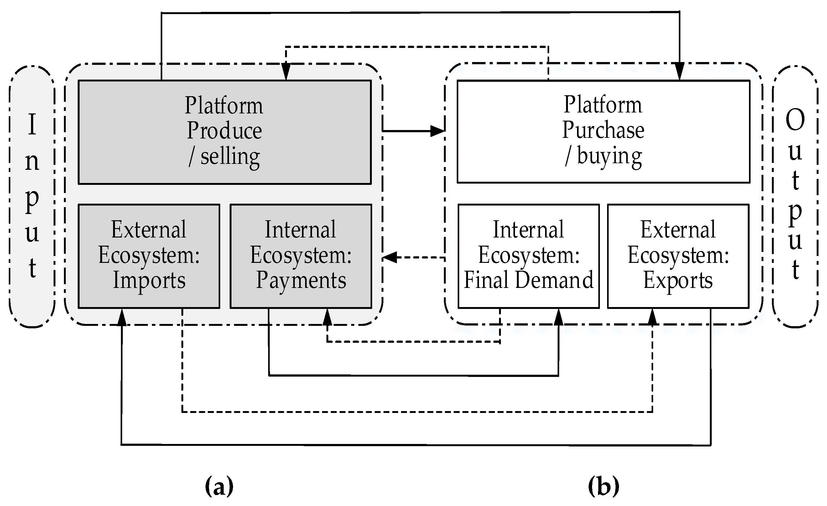
Figure 2.
Observation, regression equations, and equilibrium of the platform produce/selling and purchase/buying transactions in the financial and insurance activities industry.
Figure 2.
Observation, regression equations, and equilibrium of the platform produce/selling and purchase/buying transactions in the financial and insurance activities industry.
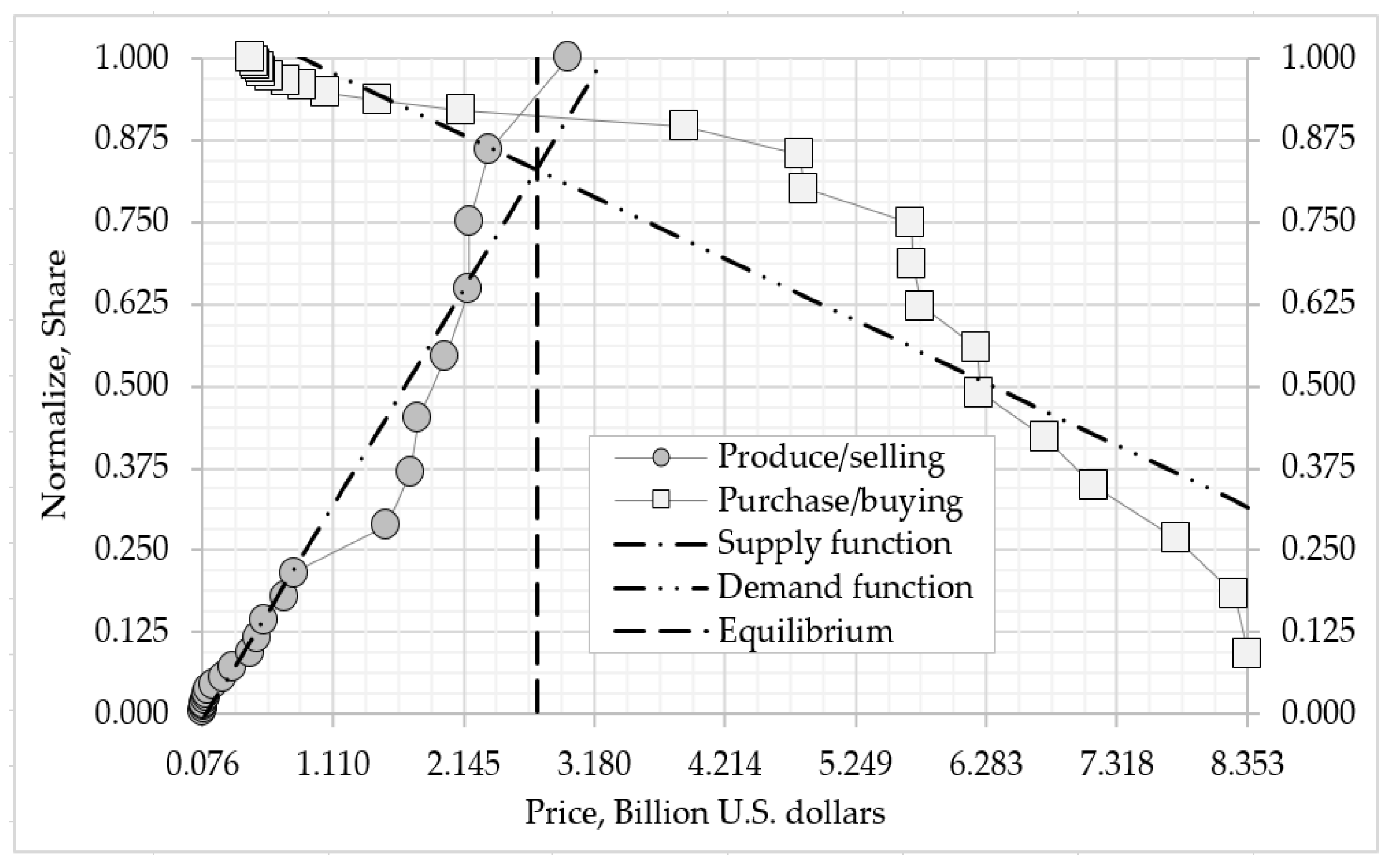
Figure 4.
Observation, regression equations, and equilibrium of the internal ecosystem payment and final demand transactions in the financial and insurance activities industry.
Figure 4.
Observation, regression equations, and equilibrium of the internal ecosystem payment and final demand transactions in the financial and insurance activities industry.
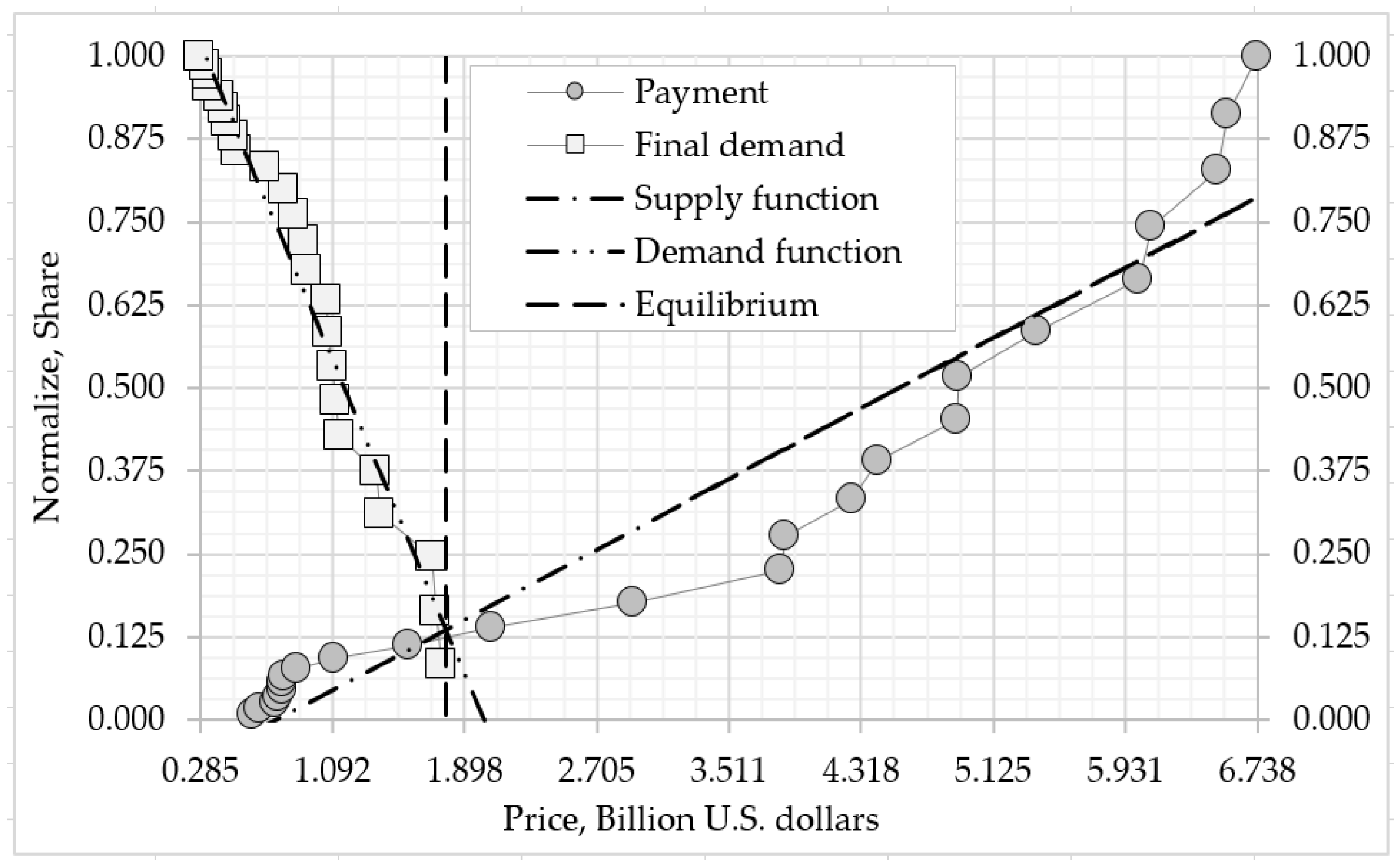
Disclaimer/Publisher’s Note: The statements, opinions and data contained in all publications are solely those of the individual author(s) and contributor(s) and not of MDPI and/or the editor(s). MDPI and/or the editor(s) disclaim responsibility for any injury to people or property resulting from any ideas, methods, instructions or products referred to in the content. |
© 2025 by the authors. Licensee MDPI, Basel, Switzerland. This article is an open access article distributed under the terms and conditions of the Creative Commons Attribution (CC BY) license (http://creativecommons.org/licenses/by/4.0/).
Copyright: This open access article is published under a Creative Commons CC BY 4.0 license, which permit the free download, distribution, and reuse, provided that the author and preprint are cited in any reuse.


