
Submitted:
19 August 2025
Posted:
19 August 2025
You are already at the latest version
Abstract
Urban systems are increasingly challenged by the complex interplay of social, economic, environmental, and infrastructural dynamics. Traditional methods typically focus on isolated impacts, failing to adequately account for the interconnectedness of urban subsystems. This paper addresses this research gap by leveraging system dynamics as a robust modeling and simulation methodology for exploring urban developmental patterns and their long-term implications. The approach is contextualized within the sustainable development discourse, emphasizing systemic feedback relationships among transport, population, economy, and environment subsystems. We demonstrate the method's efficacy through an in-depth case study of Mandra, Greece, a city facing typical urban challenges such as congestion, economic stagnation, and environmental degradation. The developed simulation model establishes clear causal links among key variables, enabling scenario testing and long-term forecasting of policy impacts. Results from diverse scenarios illustrate how various urban development policies might affect system sustainability over extended periods. The model proves valuable for urban planners by simplifying complex urban dynamics into actionable insights, thus significantly enhancing informed decision-making. Ultimately, this study underscores the potential of system dynamics to bridge urban complexity with practical policymaking, offering an innovative analytical framework to guide cities toward sustainable futures.
Keywords:
system dynamics
; sustainability
; transportation
; urban development
; simulation
; policymaking
1. Introduction
The rapid increase of urban development and cities’ population is causing different issues to be addressed concerning different aspects of a city, such as environment, economy, and social sustainability (Bibri & Krogstie, 2017). Urban areas often face issues such as traffic congestion, inadequate infrastructure, public health concerns, energy shortages, education system shortcomings (Lee J., Phaal & Lee, S., 2013), insufficient housing, increases in crime and unemployment, deteriorating facilities, frequent power failures, and limited real-time data sharing. Addressing these challenges requires smarter approaches to improve urban living, upgrade infrastructure, and enhance services (Radek Kuchta, 2014).These new challenges concern people’s quality of life, the renewal of natural resources, and the sustainability of the urban environment. The challenge of sustainable urban development has led to “smart cities”, becoming an interesting topic of research and practice worldwide.
Since more than half of the world’s population lives in urban areas and an ever-increasing proportion of them in cities (United Nations, 2012), the problem of sustainable development now lies in the process of urban development. Cities account for roughly 70% of global resource consumption, making them the largest consumers of energy. Their high population density and concentrated socio-economic activities, coupled with inefficiencies in the built environment, also make urban areas major contributors to greenhouse gas (GHG) emissions.
Over the years, as the population has grown and cities have expanded due to the effects of globalization and increased free trade, the transportation infrastructure and systems have undergone significant growth. Yet, these significant achievements have been accompanied by notable drawbacks, leaving impacts on environmental quality, social well-being, and economic stability. The concept of sustainable development was specifically designed to assess the economic, environmental, and social consequences of human activities. A sustainable system involves the dynamic interaction of three key components: the economy, the environment, and society. When applied to transportation, this concept underscores the importance of establishing interconnected relationships between transportation and these three aspects over time.
The traditional approach to sustainability in transportation has primarily focused on isolated impacts, often neglecting feedback loops and systemic interdependencies. This limitation hinders a comprehensive understanding and effective policy development. Thus, there is a clear research gap in methodologies capable of capturing these dynamic interactions.
Finding the connections between what appear to be unconnected systems takes considerably longer than it needs to because city departments usually do not communicate frequently. A policy that proves to be destructive is typically changed only after significant harm has been done. This leads to the need for a holistic approach to the problems that arise, investigating them in a clearly defined framework (system), considering the possible influence of external variables. For a conflict resolution process to be effective, it should meet the needs and requirements of all stakeholders involved (Al-Masri et al., 2021).
For this purpose, it is essential to have frameworks or guiding principles that support the modeling and simulation of complex dynamic systems. A systems thinking perspective is particularly well-suited, as it focuses on understanding systems in their entirety rather than treating them merely as separate conceptual or analytical components. Interconnectivity and hierarchy describe the spatial and structural dimensions of a system, but systems—especially complex ones—have another dimension, the temporal one. Systems whose state and behavior change over time are referred to as dynamic systems, reflecting the significant influence of their temporal characteristics. More specifically, though, change over time is governed mathematically by a well-defined rule or set of rules, such as an equation or an algorithm. This well-defined rule also makes the system deterministic by default (Zelinka & Daher, 2021). Systems thinking is a method of studying the dynamic behavior of a complex system, taking into account the system approach, i.e., the system as a whole and not in isolation from its wider environment. Systems dynamics is a tool or field of knowledge for understanding a dynamic system’s change and complexity over time.
This study aims to develop an experimental simulation model to explore the complex and interdependent relationships between the various components within the social, economic, environmental, and transportation sectors. The model is utilized to evaluate the impacts of development policies and generate predictions over the medium to long term. It also examines the potential outcomes of various scenarios under alternative policies, which aids the government in making informed decisions about urban development policies.
2. Literature Review
Urban environments today are complex. They experience rapid growth, spatial expansion, environmental decline, and changing socio-economic conditions. These systems result from dynamic interactions among infrastructure, governance, behavior, and ecological processes. To understand and manage this complexity, we need methods that go beyond straightforward planning. We must capture the feedback-rich, path-dependent nature of cities. System Dynamics (SD) offers one such method, allowing us to simulate urban processes over time, model delays, and show how local actions lead to larger systemic consequences (Sterman, 2000). In the past decade, SD has become a common approach in urban systems research. Recent studies use SD to evaluate development scenarios, test resilience strategies, and simulate changes across different urban areas. What sets SD apart from other modeling tools is its ability to capture feedback loops, time lags, and policy ripple effects. These elements are critical to today’s urban challenges. For instance, Yeomans (2023) improves the classic SD model by adding SimDec, a sensitivity analysis tool that shows how small changes in parameters can lead to big outcomes. This promotes clearer and more flexible urban decision-making. Similarly, Yang et al. (2024) created an SD framework that includes Data Envelopment Analysis (DEA) to compare various development scenarios across social, economic, and environmental aspects. This broader view helps urban managers assess the trade-offs involved in growth strategies. These tools are very useful when cities face multiple pressures, such as economic shifts, population increases, and environmental decline. Wu and Huang (2023) modeled a spatial planning system using SD to explore how “production-living-ecological” functions interact. Their work highlights the interconnectedness of land use and urban well-being. Additionally, Hou (2025) simulated Beijing’s green productivity over ten years, showing how factors like innovation, policies, and human capital affect sustainable development over time. As cities become more unpredictable, another branch of SD modeling directly incorporates uncertainty into planning. Wu et al. (2023) introduces a probabilistic SD model that uses Monte Carlo simulations to account for uncertainty in transport, environment, and urban form relationships. These tools not only help optimize policies but also visualize long-term risks and adaptive pathways. This growing body of research shows that SD is not just for conceptual mapping or sector-specific models. It acts as a platform for integrated, long-term scenario testing, allowing decision-makers to experiment with policy options safely before putting them into practice. Beyond high-level development models, SD effectively models vital urban subsystems, especially transportation. Mylonakou et al. (2023) highlighted that transportation strongly connects to land use, air quality, and spatial equity. By integrating transport into a larger SD model, the study aims to show how small adjustments—like shifts in transportation modes or pricing strategies—can lead to significant social and environmental impacts. Alipouri et al. (2023) further support this idea by demonstrating that land use and mobility must be examined together to create just and efficient urban spaces. Suryani et al. (2020) used SD to examine how the dynamic interplay of economic, environmental, and social factors shapes the overall sustainability of transportation systems. Nunes et al. (2021) combine cognitive mapping and the system dynamics approach to find which factors foster smart city success, as well as the cause-and-effect relationships among these determinants. Meanwhile, Moradi and Vagnoni (2018) studied low-carbon mobility pathways, offering insights into changes within urban transport systems. Lara et al. (2023) used causal loop diagrams to aid collaboration between transport and spatial planning, illustrating that SD models can facilitate both technical assessments and participatory governance. These examples highlight that SD is adaptable. It spans from infrastructure planning to engaging stakeholders, creating a shared language for understanding trade-offs and anticipating unintended effects. As cities confront climate changes, economic shocks, and governance issues, SD increasingly models resilience and systemic sustainability. Datola et al. (2022) proposed a Sustainable Development Model (SDM) that uses SD to explore the connections among governance structures, environmental quality, infrastructure strength, and social equity. Their model acts as a guide for cities aiming to move from static risk evaluations to dynamic resilience planning.
Together, these studies demonstrate that SD is effective for analyzing urban complexity. They show that SD can capture the cumulative, delayed, and non-linear effects of urban decisions. These qualities are crucial for long-term planning in unstable conditions. However, challenges remain. Many current SD models focus only on single sectors, making it hard to evaluate interdependencies. Others are too vague and don’t respond well to local cultural, spatial, or behavioral contexts. What we need is a dynamic modeling environment that simulates how various urban subsystems—mobility, environment, population, economy—interact, evolve, and respond to different policy approaches. We also require models that connect these systemic behaviors directly to planning tools, allowing policymakers to foresee synergies, trade-offs, and risks over time and space.
In light of these research gaps, this study will use System Dynamics as the main method for modeling urban complexity. The goal is to create a simulation environment that reflects feedback loops, non-linear interactions, and time delays among key subsystems: transportation, population, economy, and environment. Unlike sector-specific models, this approach offers a holistic view of the city, enabling stakeholders to simulate and compare different development paths. To implement the model, specialized SD software like Vensim, has been utilized. The result will be a decision-support tool aimed at urban authorities and planners, enabling them to explore “what-if” scenarios, quantify trade-offs, and align policy choices with sustainability and resilience goals. More than just a technical solution, the model will serve as a cognitive aid, helping stakeholders understand the city as a connected system rather than a collection of separate parts.
This paper is constructed as follows. The case study and the indicators employed in the model are outlined in Section 1, which pertains to the development of the system dynamics model. In Section 2, the research objectives are addressed by the use of causal loop modeling. The subsequent section outlines the methodology that aims to achieve a more accurate representation of the problem, along with the mathematical equations incorporating several variables used in the model, to develop a model that can effectively analyze real-world data. The dynamic model is finalized after creating the equations and computing the values of each variable. The following section presents the baseline scenario and many suggestive scenarios, which aim to evaluate different tactics and initiatives implemented by the local authorities. In the last section, the findings and conclusions are presented, along with potential future additions that could be implemented.
3. Proposed Model
3.1. Methodology
The study presents a model that focuses on a tool for evaluating the influencers and causal links within a city’s systems. It proposes a novel approach for assessing the impacts of new practices or policies and can significantly contribute to the decision-making process. The application of this model to any municipality or city can be effortlessly accomplished by inputting the relevant data on each occasion. Equations, variables, and feedback loops are all used in SD approaches. The causal loop graphic (Figure 1) illustrates how the feedback loops work. Stock, flow, and auxiliary variables are among the variables.
- A stock, also called a level variable, represents the condition of a system element that gathers or holds a flow over a given period.
- The flow, or rate variable, reflects how much the stock changes, either increasing or decreasing, during that period.
- The rate that defines a flow is determined by related factors known as auxiliary variables.Other integral, differential, or other equations connect all of these variables (Asasuppakit & Thiengburanathum, 2020).
To strengthen systems thinking and enhance learning, the system should be both modeled and simulated. Bala et al. (2016) outline six key phases for developing a system dynamics model: starting with identifying and defining the problem, then designing the system, formulating the model, testing and evaluating it, applying and implementing the model, sharing the outcomes, and creating suitable strategies or infrastructure informed by the results.
In this study, the procedure adopted to model and simulate these complex systems through a systems-thinking lens included the following steps:
- 1.
- Problem identification and system understanding.
- 2.
- Identification of subsystems and causal relationships.
- 3.
- System structure visualization using causal diagrams (qualitative analysis).
- 4.
- Analysis of relationships between system variables (quantitative analysis).
- 5.
- Scenario modelling.
- 6.
- Simulation results evaluation.
In this study, the city of Mandra, the former municipality in West Attica (Greece), was selected as a case study. This study employed the Vensim PLE System Dynamics software for modeling and simulation tasks. Vensim enables users to create models through a visual interface that incorporates flowcharts and causal diagrams, supported by a declarative, equation-based programming structure. Figure 2 illustrates the methodological workflow followed in this research.
3.1.1. Identification of the Urban Subsystems
The city of Mandra, located in West Attica, Greece, is characterized by a population of approximately 15,000 residents. The city faces typical urban challenges, such as traffic congestion, economic stagnation, and environmental stress, making it an ideal context for exploring urban system dynamics.
Figure 3.
Main transportation routes and landmarks in Mandra.
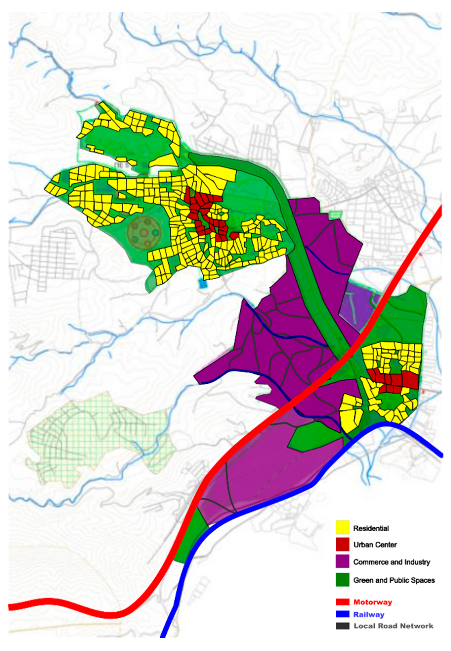
Table 1 shows a brief description of each subsystem that makes up the urban system under study, along with some variables that help approach them. The selected subsystems are:
- Society
- Economy
- Transportation/s
- Environment
To better understand the model, some basic assumptions must be defined. These are initially listed as follows:
- Urbanization is a complex and dynamic system that presents a range of interconnected problems that require systemic solutions. The urban system can be studied through the prism of four main domains: the domain of society, economy, environment and transportation
- These areas come into contact and are connected through certain factors.
- The deeper internal micro-mechanism between actors is ignored in the model.
- To focus the study on human activity, the effect of physical changes (laws of nature) on the system in the short term is considered negligible.
- The model disregards random effects due to limited data availability and the little impact of randomness on the fundamental behavioral patterns. Consequently, mean values are allocated to all parameters and inputs.
The proposed framework, built with a system dynamics approach, is composed of two main components. The first is a causal loop diagram (CLD) illustrating the cause-and-effect interactions among the different subsystems. The second is a stock–flow diagram that depicts the quantitative linkages between the model’s variables. The concept of the stock and flow diagram of selected variables is described mathematically below (Duggan, J., 2016):
where Inflow and Outflow are the inventory inflow and outflow, respectively.
If the focus was on the flows and not the stocks, then equation [1] could be expressed as follows:
3.1.2. Qualitative Analysis (Causal Loop Diagram)
The most critical step in the development of a model using system dynamics is the creation of a “map” of the system, including all parameters as well as the relationships between them (interactions). In this phase of the analysis, the primary purpose is to identify some key variables that influence the identified pillars, as well as their expected effect on them (positive or negative). This mapping is a basis for the search for more relationships through new variables in the studied subsystems. This means that the qualitative capture could contain more and more variables with which the model would become more and more complex, but also more accurate. However, in the context of this analysis, we consider this extent satisfactory for the level of analysis we are interested in, and more variables will be referred to more extensively in the quantitative analysis phase.
3.1.3. Quantitative Analysis
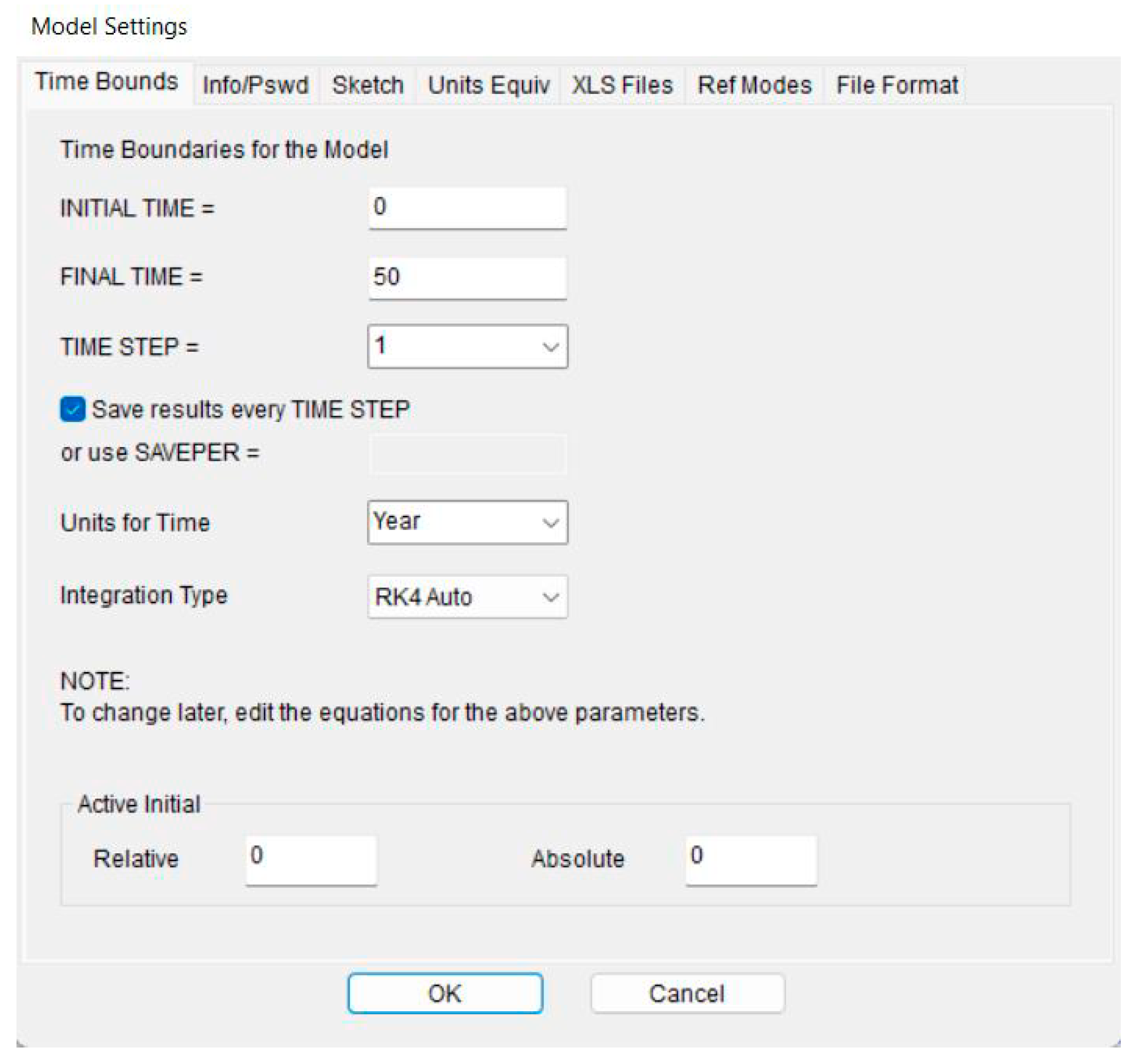
In the quantitative representation of the model, the initial conditions were first defined. The present study explores the simulation of the system for a duration of 50 years, with an analysis step of one year. The 4th-order Runge-Kutta method was chosen for the calculations, as it provides more accurate mathematical results for the desired level of analysis. Figure. 4 depicts the initial conditions definition window in Vensim.
Figure 4.
Initial conditions setting in Vensim.
Using the toolbar offered in this program, an urban system was mapped. Using the toolbar offered in this program, an urban system was mapped. The main variables considered in this system are the city population, active workforce, individual income, public means of transport fleet, number of motorized vehicles, and pollutant emissions.
Figure 5 shows a Stock and Flow Diagram (SFD) created in Vensim, intended to clarify the complex, non-linear relationships in urban systems. The model starts simulations with an initial population of 15,000 people over a 50-year period. To address the common issue of limited data at the urban level, we scaled down national economic indicators, specifically GDP data from Greece (1981–2021), to maintain local relevance. This model incorporates six key stock variables—City Population, Active Workforce, Individual Income, Public Transport Fleet, Motorized Trips, and Pollutant Emissions. Each variable is affected by specific inflow and outflow processes. Internal feedback mechanisms and external factors, such as CO₂ absorption rates in urban green spaces and demographic migration rates influence these flows. Using historical averages for parameterization strengthens the model and allows for its use in different urban settings. The model’s strength lies in its use of reinforcing and balancing feedback loops, described in Annex II. These loops capture the subtle yet essential behaviors and feedback processes found in complex adaptive urban systems. This feedback structure enables the study of non-linear dynamics, policy resistance, and delayed reactions—elements often overlooked by traditional linear models. This improves the analytical depth and predictive accuracy of the findings. Moreover, the model offers a new logical framework through its integrated, multi-sector approach. It captures the co-evolutionary dynamics among demographic, economic, transportation, and environmental systems. This integration allows for a simultaneous analysis of various urban processes, revealing insights into combined or conflicting policy effects that single-sector models might miss. The model’s effectiveness comes from its strong methodology and adaptability, allowing for detailed scenario analyses and extensive sensitivity testing. As a result, urban policymakers can use this model to reliably predict the systemic effects of proposed actions, leading to more effective, evidence-based urban sustainability strategies. All mathematical relationships and measurement units that define system dynamics are laid out in Annex I to ensure transparency and reproducibility.
4. Scenarios Development and Results
Since the model was fully rendered in Vensim, the first simulation was also done based on the values chosen as initial values for the model. The results per stock variable are presented below.
The resulting values for the population variable (Figure. 6) seem to be reasonable and reflect a realistic situation. At the end of the simulation period, based on the tables with data extracted from Vensim, projection indicates that the city’s population will reach 15,511, representing an increase of 511 residents compared to the starting figure of 15,000. This means that the variables contributing to population growth (Birth rate, Rate of immigration inflows) have been considered at a marginally higher rate than those contributing to population decline (migration outflow rate, Death rate). Accordingly, for the next stock variable, the public transport fleet, the following diagrams have been calculated (Figure 7).
As shown in Figure 7, for reasonable values of purchase rates (0.001) and attrition rates (0.02), there is an increase over time in the total number of public transport users. This happens mainly because of the need to buy new vehicles, which in turn results from the increase in the city’s population, as was seen in Figure 6. This analysis isolates the reported variables from the rest of the system. However, the relationships and interconnections in the model interrelate all the variables of the subsystems in order to achieve a rational and as realistic as possible result.
In the case of labor in Figure 8, the results are reasonable as well, based on the values and relationships that have been set. The active workforce shows a decreasing trend, as a result of the decreasing hiring rate (dependent on the lack of workers in the labor market and labor market demand parameters) and the redundancy rate (Annex 1).
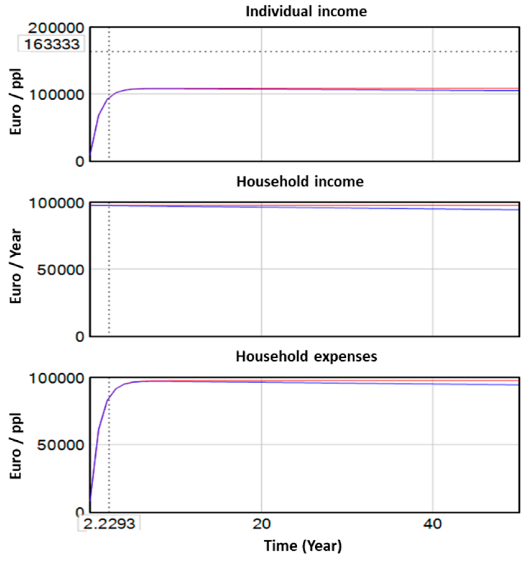
The plots of the variables shown in Figure 9 are related to individual income. The results are not logical, as on the one hand, the amounts corresponding to the individual income start from very low and end up stabilizing. This means that the proposed model does not offer a good representation of the situation. Since the values stabilize after some time, it could mean that the inputs to the specific subsystem do not have much variation, or else that some of the variables related to it also need to be modified (eg Country Population).
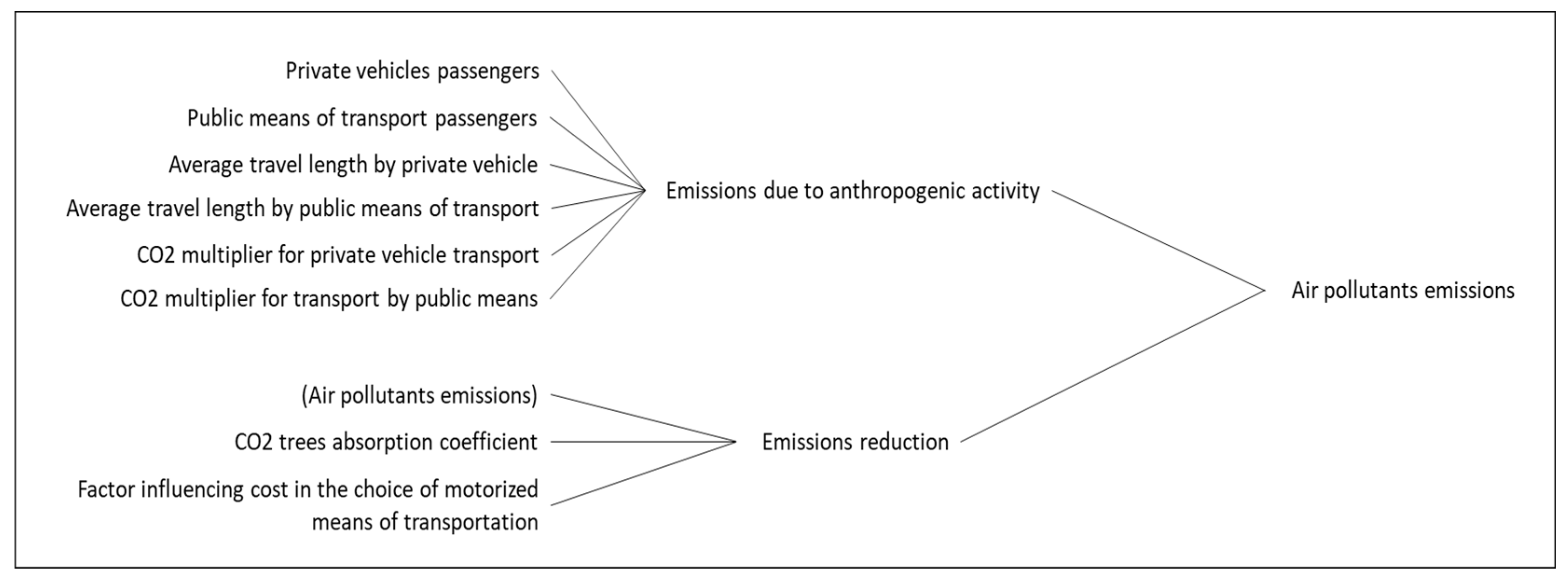
Figure 10 presents the diagram for pollutant emission. In this case, the simulation seems to have an issue in the first part, where emissions due to human activity are zeroed out. Of course, this cannot be done, as emissions due to anthropogenic activity are never going to go to zero as long as the human species survives and there is economic activity.
However, it is observed that the quantities that act as inputs to the system refer to only one side of anthropogenic activity, the one that contributes to pollution only due to transport. Therefore, the change that needs to be made is to expand the system boundaries to this subsystem and study it by considering another variable/coefficient.
Figure 11 shows the diagrams related to the number of motorized movements in a city. As can be seen, over a period of 50 years, the diagram has a parabolic shape. Towards the end of the period of interest, the results are quite large numbers, which, to some extent, is justified due to the fact that it concerns the total motorized trips per year. However, perhaps this is an indication that models of this size and scale deserve a lifespan of less than 50 years.
Since the weaknesses of the model are now known from the Baseline Scenario, 3 new scenarios arise for examination.
- Scenario 1: The population of the country is not an exogenous variable, but a Stock Variable.
- Scenario 2: Anthropogenic activity contributing to CO2 emissions is not limited to emissions resulting from transport alone.
- Scenario 3: The simulation of systems with a large number of variables needs to be done for time intervals of 5-10 years.
In Scenario 1, the population is not considered an exogenous variable but a Stock variable. This means that the influence of outside forces does not dominate the system’s behavior and that the population will be ultimately affected by the system. For the stock variable, the initial value is the population of Greece in the year 2021, and the rest of the rates of change remain the same regarding the city population. After changing the necessary elements in the model, its final form is the one shown in Figure 12.
Figure 12 shows the Stock and Flow Diagram (SFD) created for Scenario 1 in the urban systems analysis using Vensim. This diagram looks at the implications of treating the national population as an internal stock variable instead of an external parameter. This change makes the model more realistic by allowing a direct connection between urban and national demographic dynamics. The starting point for this scenario uses Greece’s national population data from 2021 while keeping other urban-specific growth rates. This shift in the modeling approach lets us explore the feedback interactions between urban and national populations. It recognizes that urban populations both affect and are affected by wider national demographic trends. By including these interactions, the model greatly improves its ability to simulate and predict complex social, economic, and environmental outcomes at various levels. The model’s strength comes from its detailed construction of feedback loops. It accurately captures the complex relationship between urban and national demographic processes. These loops allow for thorough testing of how local policies or shifts in demographics might impact national population trends and the opposite. This integration across different scales is a major improvement in urban systems modeling. Scenario 1 highlights a significant step forward in System Dynamics modeling. It provides urban planners and policymakers with a detailed, multi-layered tool that delivers realistic insights into demographic sustainability and urban development. The specific mathematical relationships that define this scenario, along with their measurement units, are fully documented in Annex I.
Figure 13.
Individual income and related variables change over 50 years for Scenario 1.
Scenario 2 considers adding new variables to the environment subsystem to better capture anthropogenic activity. In particular, it was decided to add the exogenous variable “Remaining anthropogenic activity that contributes to CO2 emission”, which was assumed to constitute the 45% (IPCC, 2022) of the total annual emissions.
The results for the diagram of interest are shown in Figure 14. The main conclusion from this diagram is that although the variables now change over time, the emissions due to commuting end up zeroing out near year 10. This results from the fact that the choice of motor vehicle in the model is affected by the cost of travel, which in the event that travel costs exceed household expenses, travel is automatically zeroed out. So, the next step would be to refine the relationships that link these variables in the model. This case, however, is not covered in the context of this analysis. Regarding the charts of the remaining Stocks and their respective inflows and outflows, the changes are negligible for this and not worth mentioning. In Scenario 3, after testing various alternatives, the choice of 5 years for the simulation was made. Specifically, Figure 15 below presents all the diagrams related to the Stock variables, including their input and output diagrams.
The simulations highlight the interconnectedness of demographic growth, economic activity, mobility patterns, and environmental performance as forces behind key urban expansion. Changes in one of these areas were shown to influence the others, highlighting the value of integrated, feedback-based modeling for decision-making. Short-time horizon simulations produced stable and actionable projections, while longer time horizons revealed extensive systemic trends and pressures on the horizon. These results offer a basis on which leverage points—i.e., strategic mobility investment, demographic planning, and environmental management—can be identified through one unified framework that supports sustainable and adaptive city planning.
Overall, the scenario analysis demonstrates the potential of system dynamics in approximating urban complexity in a manner that supports strategic, intersectoral decision-making. The integrated approach enables policymakers to anticipate more effectively direct and indirect consequences of interventions, and thus align short-term interventions with long-term resilience goals. By revealing systemic interactions and points of influence, the model is an effective decision-support tool for adaptive, data-based planning for supporting sustainable urban development.
5. Conclusions
This research offers a practical method for examining the interactions among the interconnected sectors of society, the economy, the environment, and transportation, applying principles from system dynamics (SD). The results demonstrate that SD-based simulations are effective tools for assessing the cross-sectoral and interlinked variables that influence overall performance. Such models support a holistic understanding of systems and guide the creation of policies that protect resources while allowing progress, thereby fostering a healthy environment and promoting a sustainable quality of life for generations to come. Our proposed methodology excels in identifying causal links between variables over extended periods and facilitating hypothesis testing by transforming the entire process into a stock and flow system that reflects the most critical relationships. The techniques we employ simplify and structure an expansive and intricate topic, empowering decision-makers to make more informed choices. The result is a tool that allows planners to “play” with different ideas to see how proposed actions might affect other systems within the city. System dynamics provides a framework for assessing possible outcomes and developing plans that account for both short-term and long-term effects. The Systems Dynamics (SD) approach enhances the understanding of complex systems by creating hypothetical scenarios through simulations. This process helps in constructing a robust model that can provide valuable insights for decision makers. When combined with meaningful stakeholder participation, it can leverage analytical tools to address gaps in understanding that traditional information-gathering might overlook. While maintaining the value of direct public input, decision-makers can use system dynamics to gain a fuller picture of the factors that influence urban performance. Such an approach can significantly contribute to building smarter cities—ones that better recognize the interconnections between their systems and policies, and that are capable of aligning these systems to work together more effectively than before. This is consistent with findings in previous research applying SD modeling to the city of Patras, which demonstrated similar benefits in the area of urban transport and citizen satisfaction (Mylonakou et al. 2023). Finally, from this research effort it could be concluded that should not be considered only quantitative variables such as vehicle population or consumption, and city GDP to represent sustainable development of the city, but also qualitative aspects like community values and residents’ quality of life should be incorporated to capture the true nature of sustainable urban development and well-being, supporting progress toward the Sustainable Development Goals (SDGs). Quality of life metrics can serve as a valuable addition to gross domestic product (GDP), which is typically considered the primary measure of economic and social growth. For example, in the Eurostat online publication (Eurostat Statistics), for each quality-of-life dimension, a set of selected relevant indicators is presented and analysed. The pilot model developed in this work is dynamic in nature and offers the flexibility to incorporate additional sectors, such as the energy domain, demonstrating its capacity for expansion. Each sector could also be explored in greater detail by integrating more specific indicators. Future investigations should also consider embedding a cost equation within the model. The ability to replicate this model is a significant advantage as its structure can be adapted to various urban contexts by adjusting specific parameters and initial conditions to match local situations. This flexibility boosts the model’s potential value. It offers urban planners and policymakers a strong analytical tool that can be applied in various settings. The clear documentation of mathematical relationships, feedback loops, and measurement units ensures easy replication and validation, supporting comparative analyses across different urban areas. Thus, the model provides immediate practical insights while establishing a versatile framework for ongoing research and continuous improvement in urban sustainability and planning practices
Author Contributions
Conceptualization, Stylianos Karatzas, Vasiliki Lazari and Ioanna Kassa; Data curation, Stylianos Karatzas and Ioanna Kassa; Formal analysis, Stylianos Karatzas, Vasiliki Lazari and Ioanna Kassa; Methodology, Stylianos Karatzas, Vasiliki Lazari and Ioanna Kassa; Software, Ioanna Kassa; Supervision, Stylianos Karatzas and Athanasios Chassiakos; Validation, Ioanna Kassa; Writing—original draft, Stylianos Karatzas and Vasiliki Lazari; Writing—review & editing, Athanasios Chassiakos.
Funding Information: This research received no funding.
Data Availability: The original contributions presented in this study are included in the article/supplementary material. Further inquiries can be directed to the corresponding author(s).
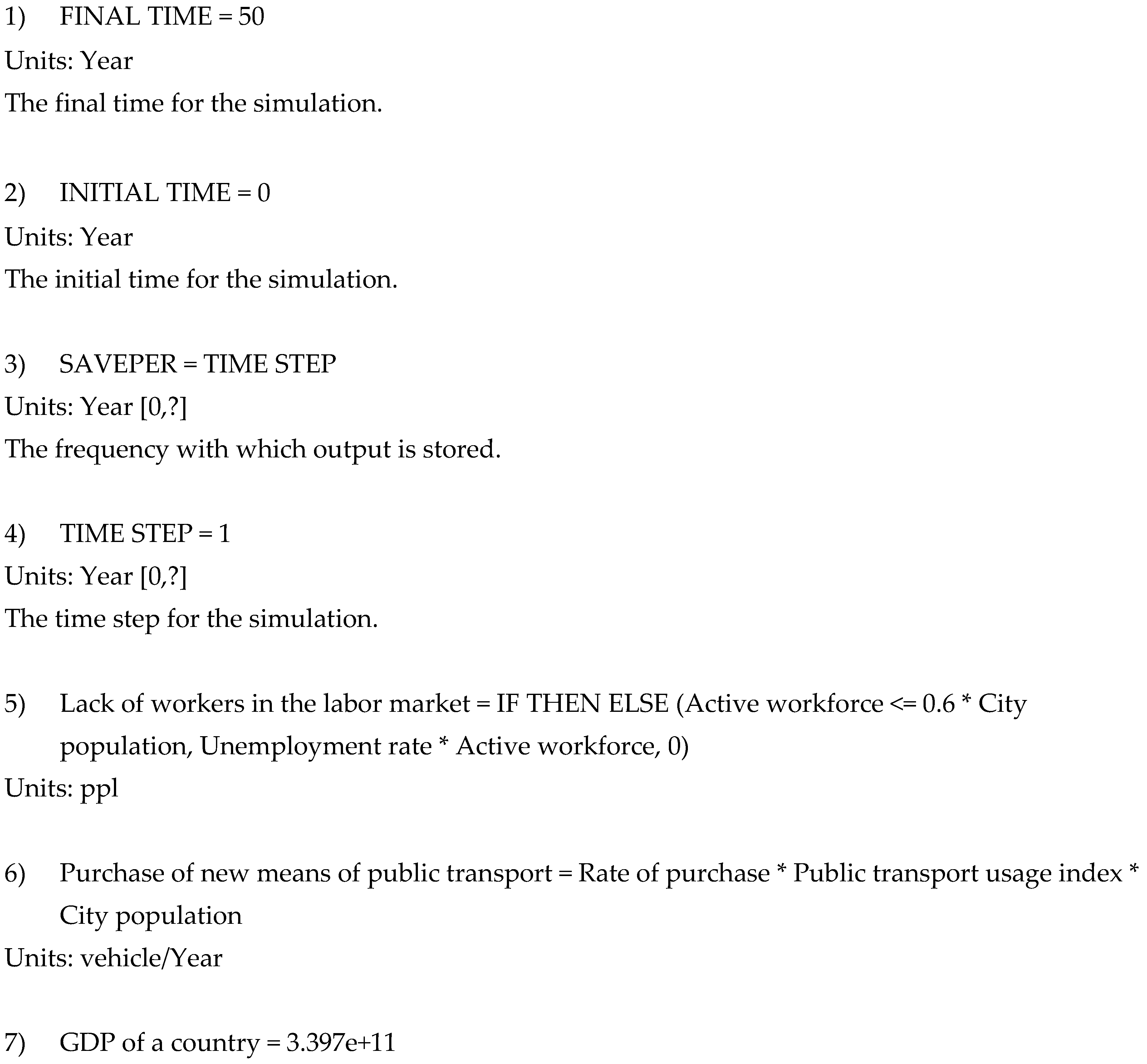
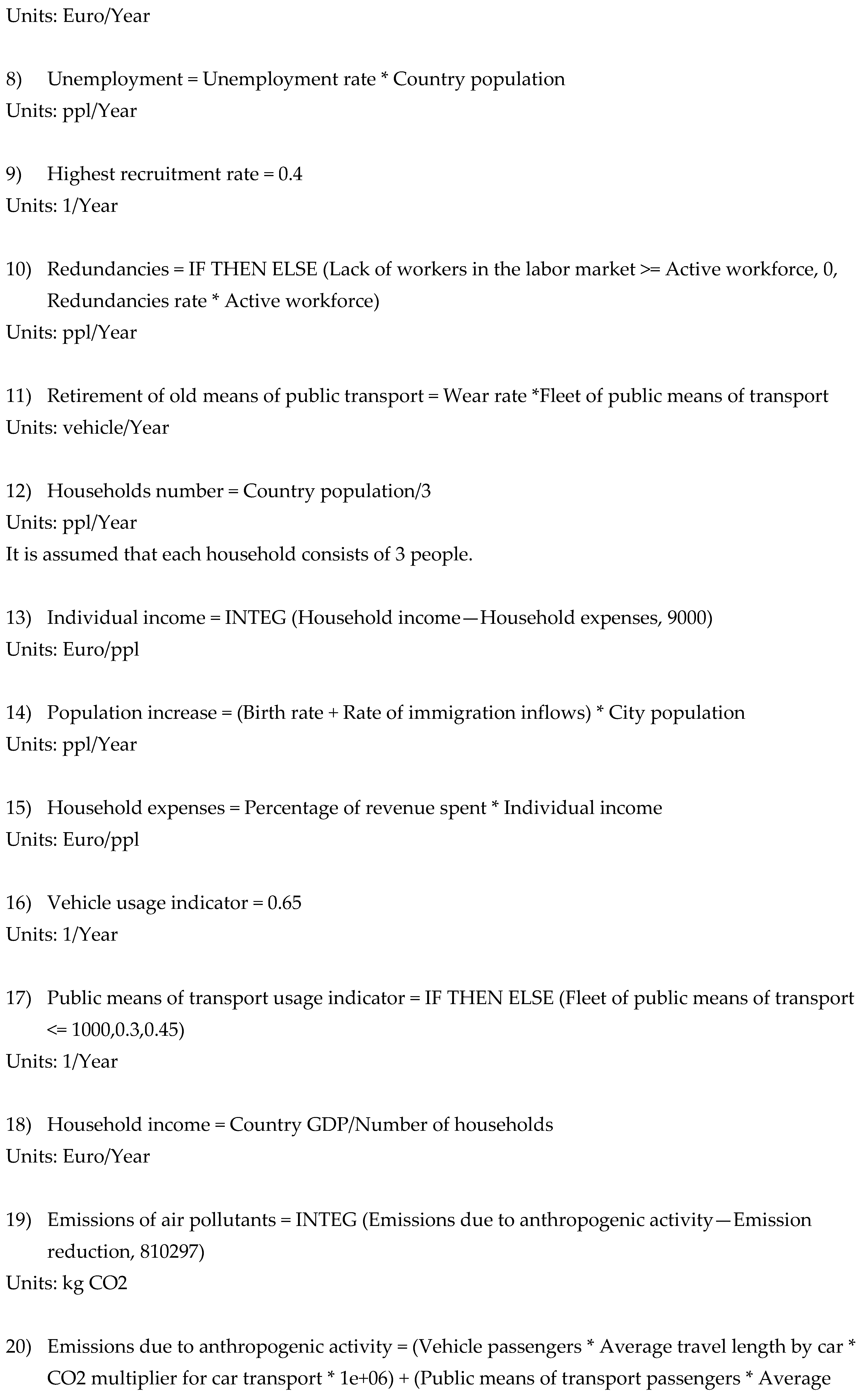
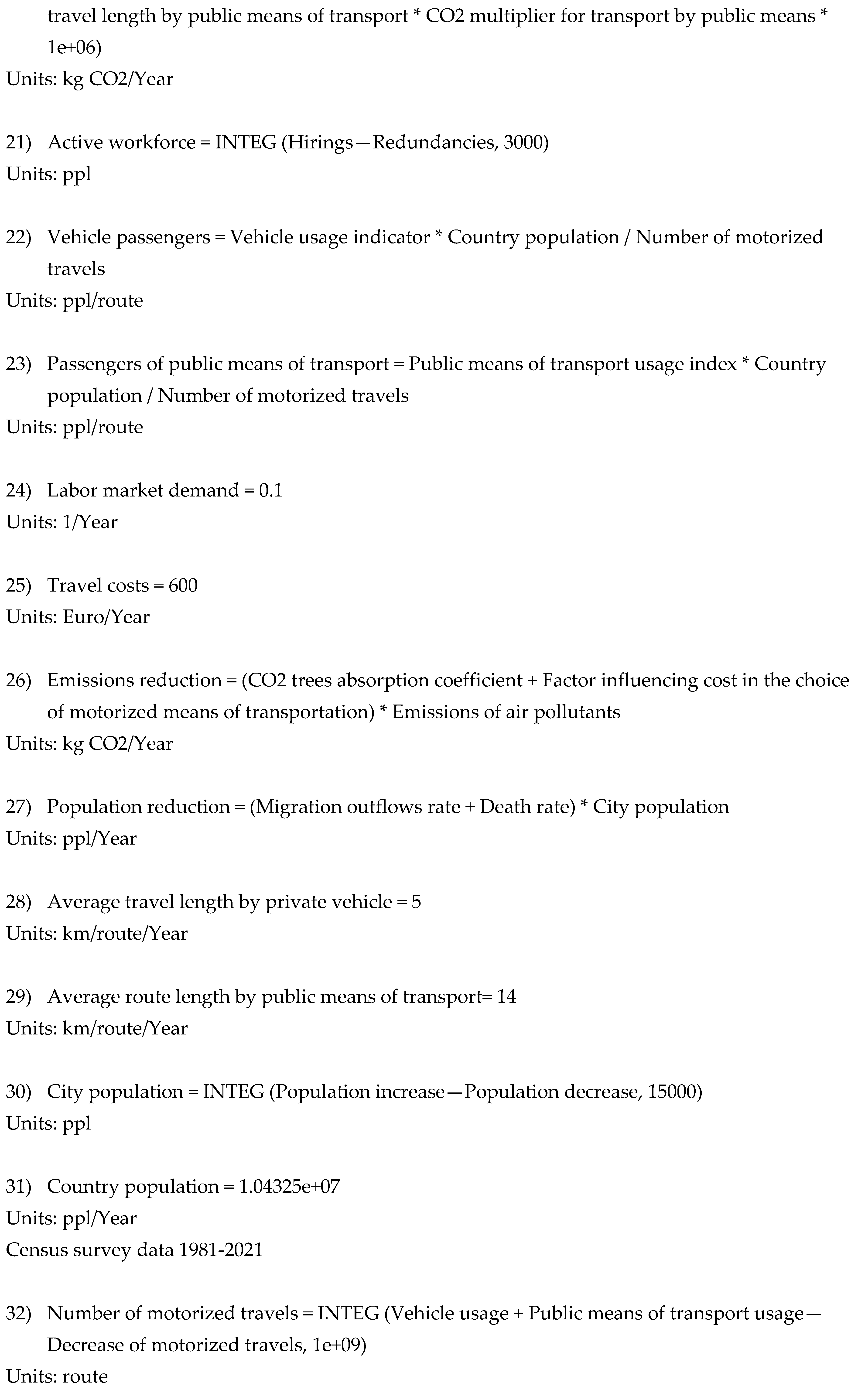
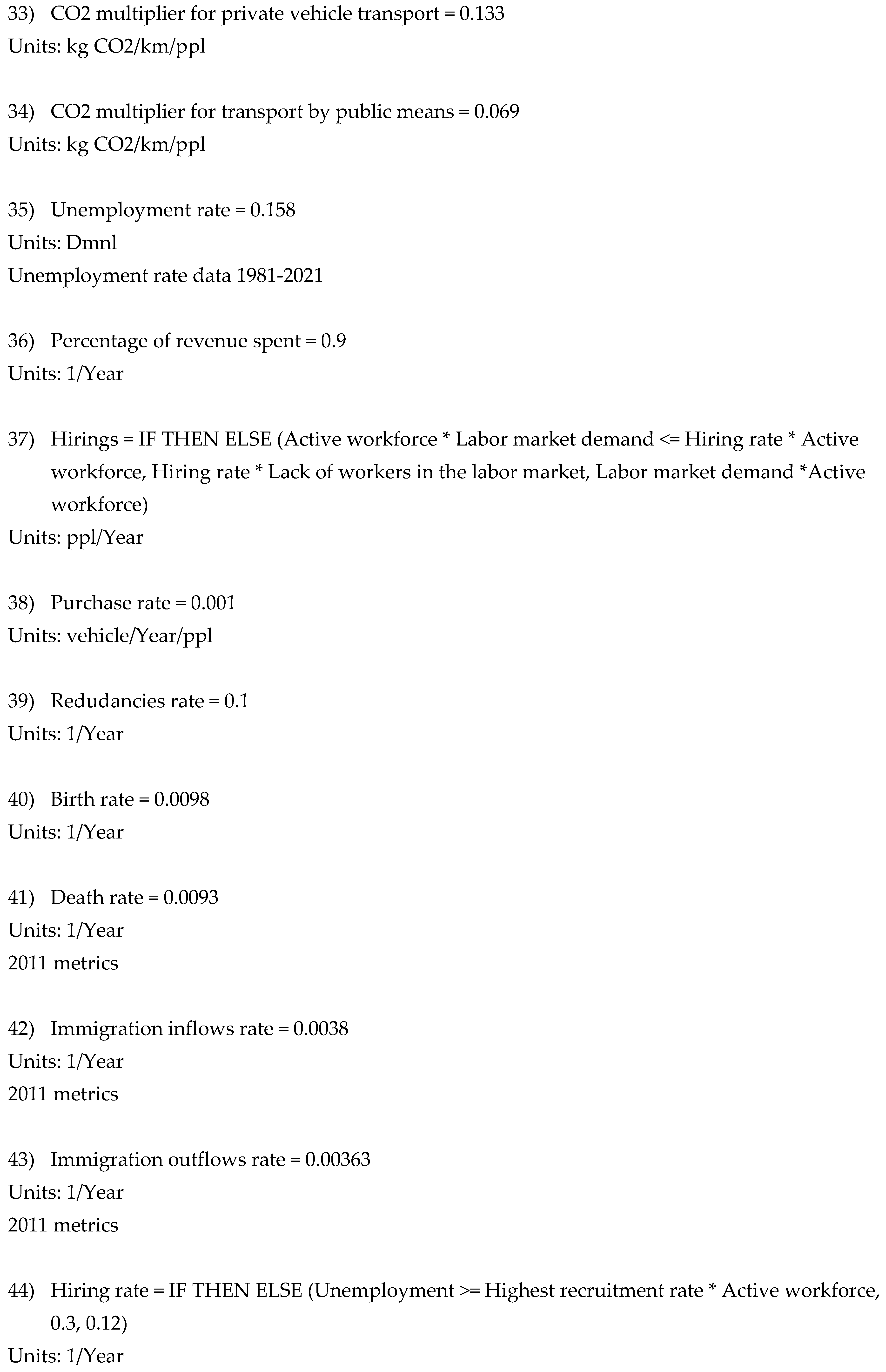
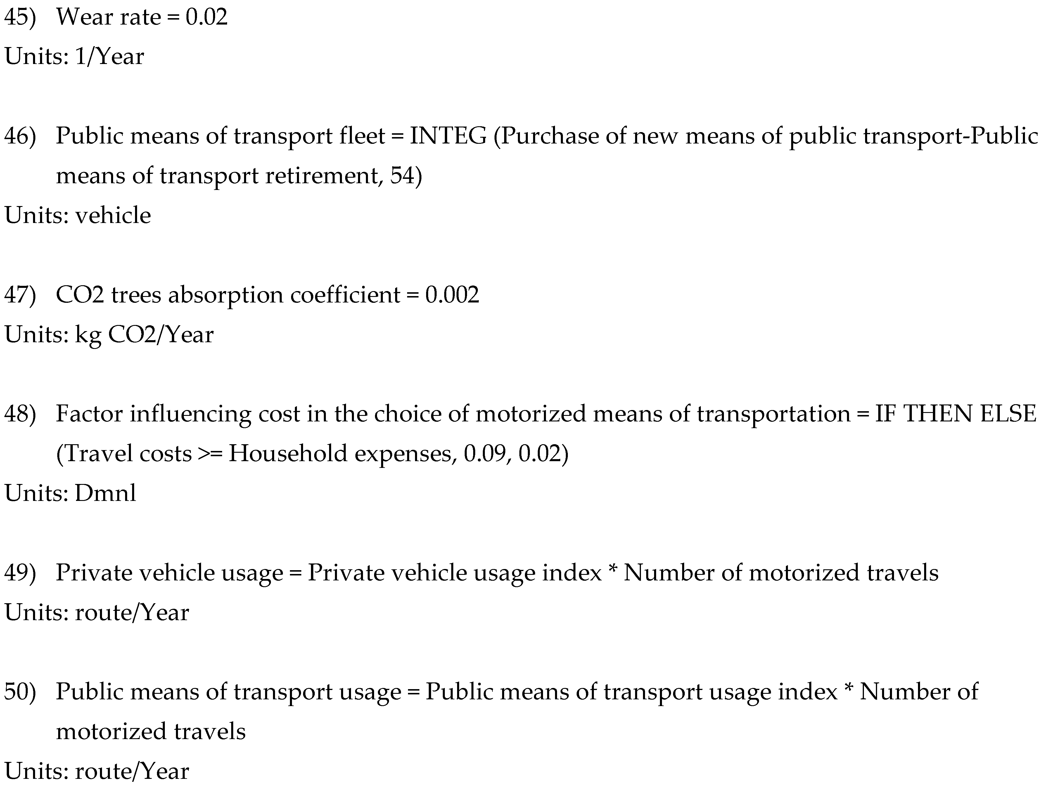
Appendix A—Mathematical Relationships Used in Vensim for the Baseline Scenario:
Appendix B—Casual Loops per Stock Variable
Figure A1.
Causal Loop for the stock variable: City population.
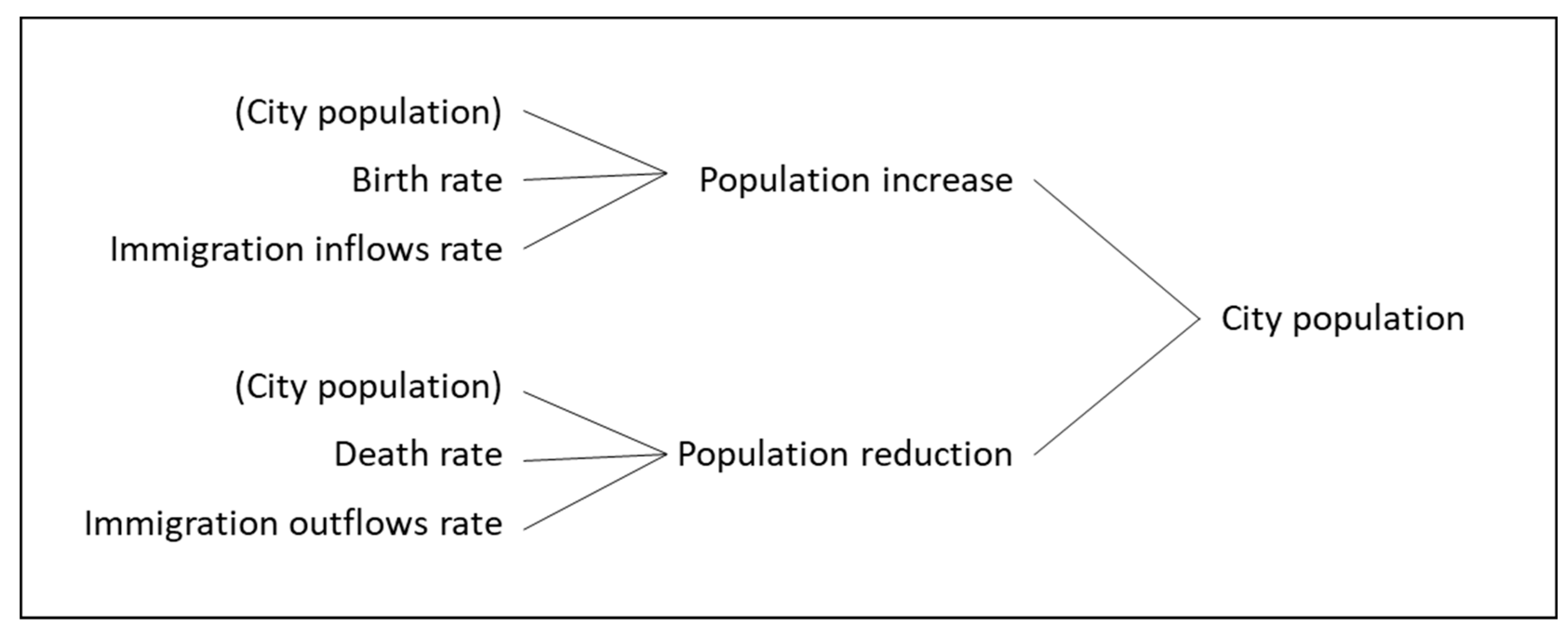
Figure A2.
Causal Loop for the stock variable: Active workforce.
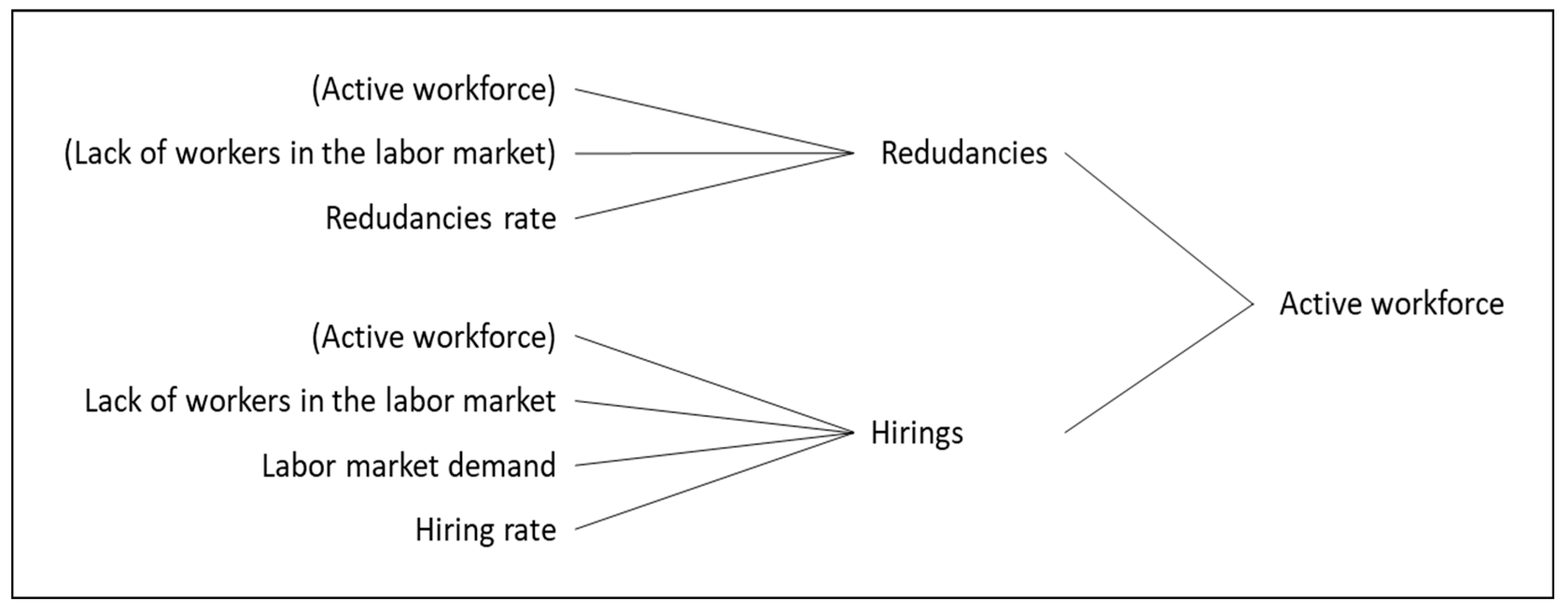
Figure A3.
ausal Loop for the stock variable: Individual income.
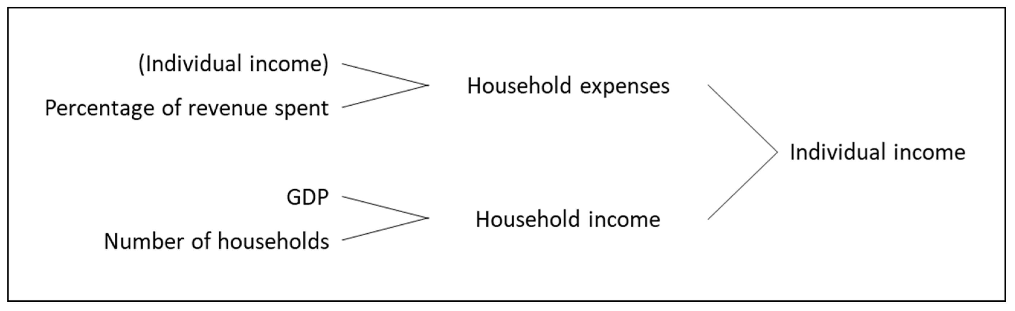
Figure A4.
Causal Loop for the stock variable: Public means of transport fleet.
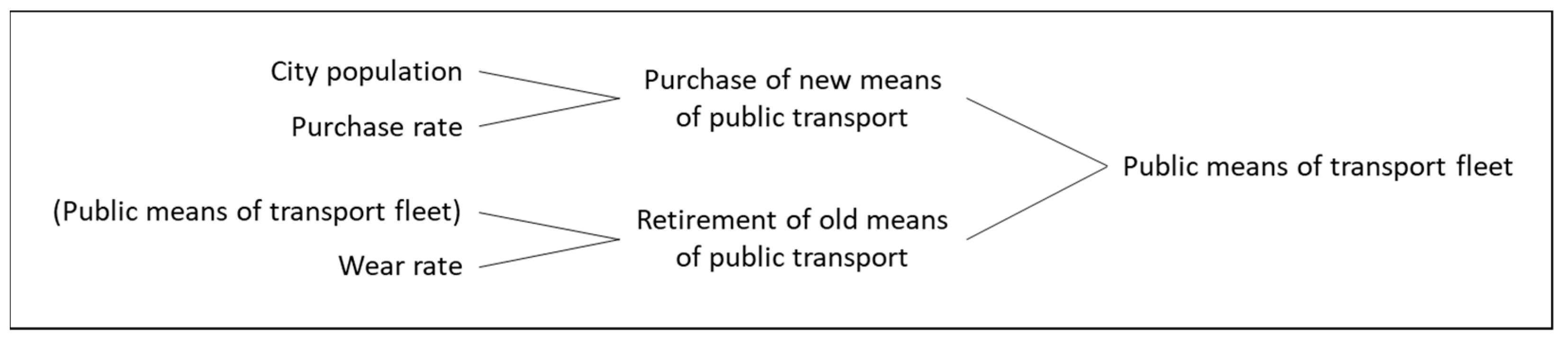
Figure A5.
Causal Loop for the stock variable: Number of motorized travels.
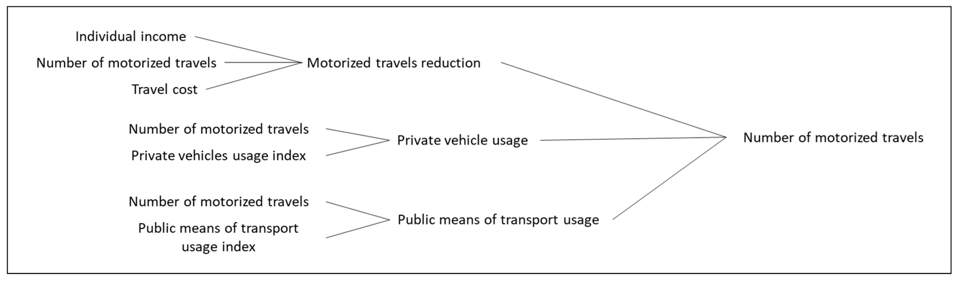
Figure A6.
Causal Loop for the stock variable: Air pollutants emissions.
References
- Al-Masri, R. A., Spyridopoulos, T., Karatzas, S., Lazari, V. M., & Tryfonas, T. (2021). A Systems Approach to Understanding Geopolitical Tensions in the Middle East in the Face of a Global Water Shortage. International Journal of System Dynamics Applications, 10(4), 1–23. [CrossRef]
- Alipour, D., & Dia, H. (2023). A Systematic Review of the Role of Land Use, Transport, and Energy-Environment Integration in Shaping Sustainable Cities. Sustainability, 15(8), 6447. https://doi.org/10.3390/su15086447.
- Bala, B. K., Arshad, F. M., & Noh, K. M. (2017). Tests for Confidence Building. Springer Texts in Business and Economics. [CrossRef]
- Bibri, S. E., & Krogstie, J. (2017). Smart sustainable cities of the future: An extensive interdisciplinary literature review. Sustainable Cities and Society, 31, 183–212. [CrossRef]
- Castellacci, F. (2017). Co-evolutionary growth: A system dynamics model. Economic Modelling, 70, 272–287. [CrossRef]
- Datola, G., Bottero, M., De Angelis, E., & Romagnoli, F. (2022). Operationalising resilience: A methodological framework for assessing urban resilience through System Dynamics Model. Ecological Modelling, 465, (. [CrossRef]
- Duggan, J. (2016). An Introduction to System Dynamics. In: System Dynamics Modeling with R. Lecture Notes in Social Networks. Springer, Cham. [CrossRef]
- Eurostat Statistics, Quality of Life Indicators, Retrieved from https://ec.europa.eu/eurostat/statistics-explained/index.php?title=Quality_of_life_indicators.
- Hou, C. (2025). Analysis of the factors promoting urban green productivity using a system dynamics simulation. Scientific Reports, 15(1), 27928.
- 2022; 10. IPCC, Climate Change 2022 Mitigation of Climate Change, Intergovernmental Panel on Climate Change, 2022, Retrieved from.
- https://www.ipcc.ch/report/ar6/wg3/downloads/report/IPCC_AR6_WGIII_SPM.pdf.
- J.W. Forrester Principies of Systems. Text and Workbook, Chapters 1 through 10. Second Preliminary Edition. Cambridge (Mass.), Wright-Allen Press, Inc., 1971, pagination irrégulière, (1973). In Recherches économiques de Louvain (Vol. 39, Issue 4, pp. 518–519). CAIRN. [CrossRef]
- Lara, D. V. R., Pfaffenbichler, P., & da Silva, A. N. R. (2023). Modeling the resilience of urban mobility when exposed to the COVID-19 pandemic: A qualitative system dynamics approach. Sustainable Cities and Society, 91. (. [CrossRef]
- Lee, J. P., Phaal, R., & Lee, S. (2013). An integrated service-device-technology roadmap for smart city development. Technological Forecasting and Social Change, 80(2), 286–306. [CrossRef]
- Li, C. Y., Wang, J. H., Zhi, Y. R., Wang, Z. R., & Gong, J. H. (2018). Simulation of the chlorination process safety management system based on system dynamics approach. Procedia engineering, 211, 332-342. [CrossRef]
- Moradi, A., & Vagnoni, E. (2018). A multi-level perspective analysis of urban mobility system dynamics: what are the future transition pathways?. Technological Forecasting and Social Change, 126, 231-243. [CrossRef]
- Mylonakou, M., Chassiakos, A. P., Karatzas, S., & Liappi, G. (2023). System Dynamics Analysis of the Relationship between Urban Transportation and Overall Citizen Satisfaction: A Case Study of Patras City, Greece. Systems, 11(3), 112. [CrossRef]
- Novotný, R., Kuchta, R., & Kadlec, J. (2014). Smart City Concept, Applications and Services. Journal of Telecommunications System & Management, 03(02). [CrossRef]
- Nunes, S., Ferreira, J. J., Govindan, K., & Pereira, L. F. (2021). “Cities go smart!”: A system dynamics-based approach to smart city conceptualization. Journal of Cleaner Production, 313, 127683. [CrossRef]
- Praopun Asasuppakit, & Poon Thiengburanathum. (2020). System dynamics model of co2 emissions from urban transportation in chiang mai city. GEOMATE Journal, 18(68), 209–216. Retrieved from https://geomatejournal.com/geomate/article/view/564.
- Sterman, J. D. (2000). Business Dynamics: Systems Thinking and Modeling for a Complex World. Boston: Irwin/McGraw-Hill.
- Suryani, E., Hendrawan, R. A., Adipraja, P. F. E., & Indraswari, R. (2020). System dynamics simulation model for urban transportation planning: a case study. International Journal of Simulation Modelling, 19(1), 5-16. [CrossRef]
- United Nations. (2012). World Urbanization Prospects The 2011 Revision. New York: Department of Economic and Social Affairs. Population Division. Retrieved from https://www.un.org/en/development/desa/population/publications/pdf/urbanization/WUP2011_Report.pdf.
- Ventana Systems. (n.d.). Vensim software. https://vensim.com.
- Wu, J., & Huang, J. (2023). A system dynamics-based synergistic model of urban production-living-ecological systems: An analytical framework and case study. Plos one, 18(10), e0293207.
- Wu, M., Wang, J., Zhang, Y., & Zhang, L. (2023). Modeling, assessment, and optimization of urban sustainability using probabilistic system dynamics. Journal of Building Design and Environment, 1(3), 8993-8993.
- Yang, L., Ma, Y., & Lou, K. (2024). Urban Development Scenario Simulation and Model Research Based on System Dynamics from the Perspective of Effect and Efficiency. Systems, 12(7), 259. [CrossRef]
- Yeomans Julian Scott, Kozlova Mariia, Extending system dynamics modeling using simulation decomposition to improve the urban planning process, Frontiers in Sustainable Cities, Volume 5—2023, 2023, DOI=10.3389/frsc.2023.1129316.
Figure 1.
The stock, flow and auxiliary variables (Li et al., 2020).
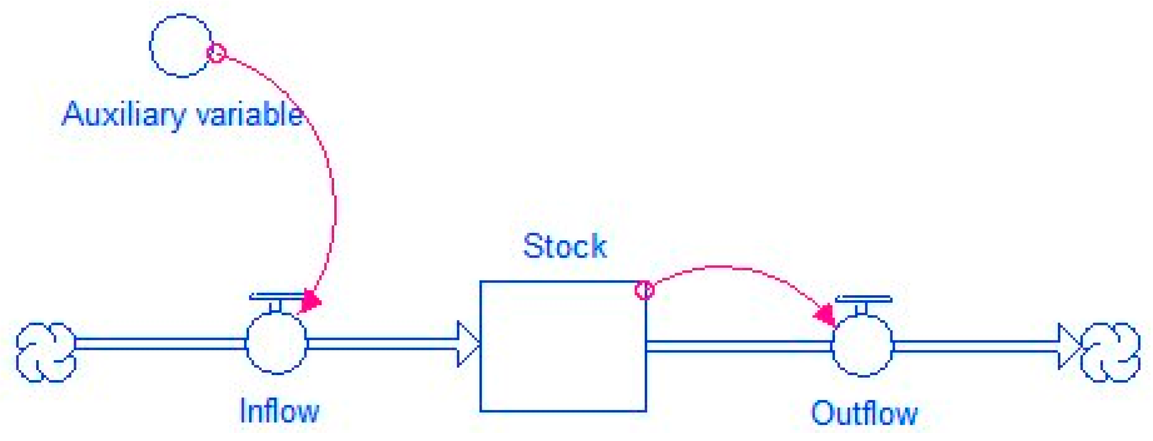
Figure 2.
Systems analysis process developed through the System Dynamics methodology.
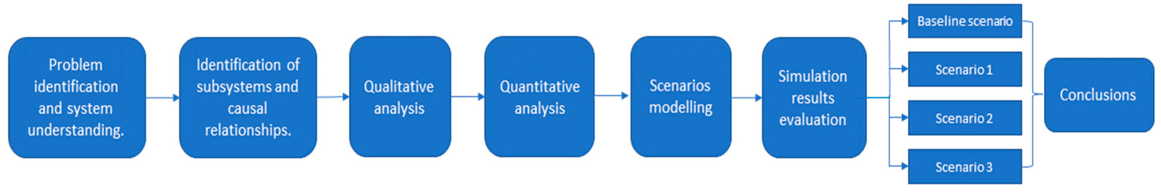
Figure 5.
Stock–flow representation of the urban system.
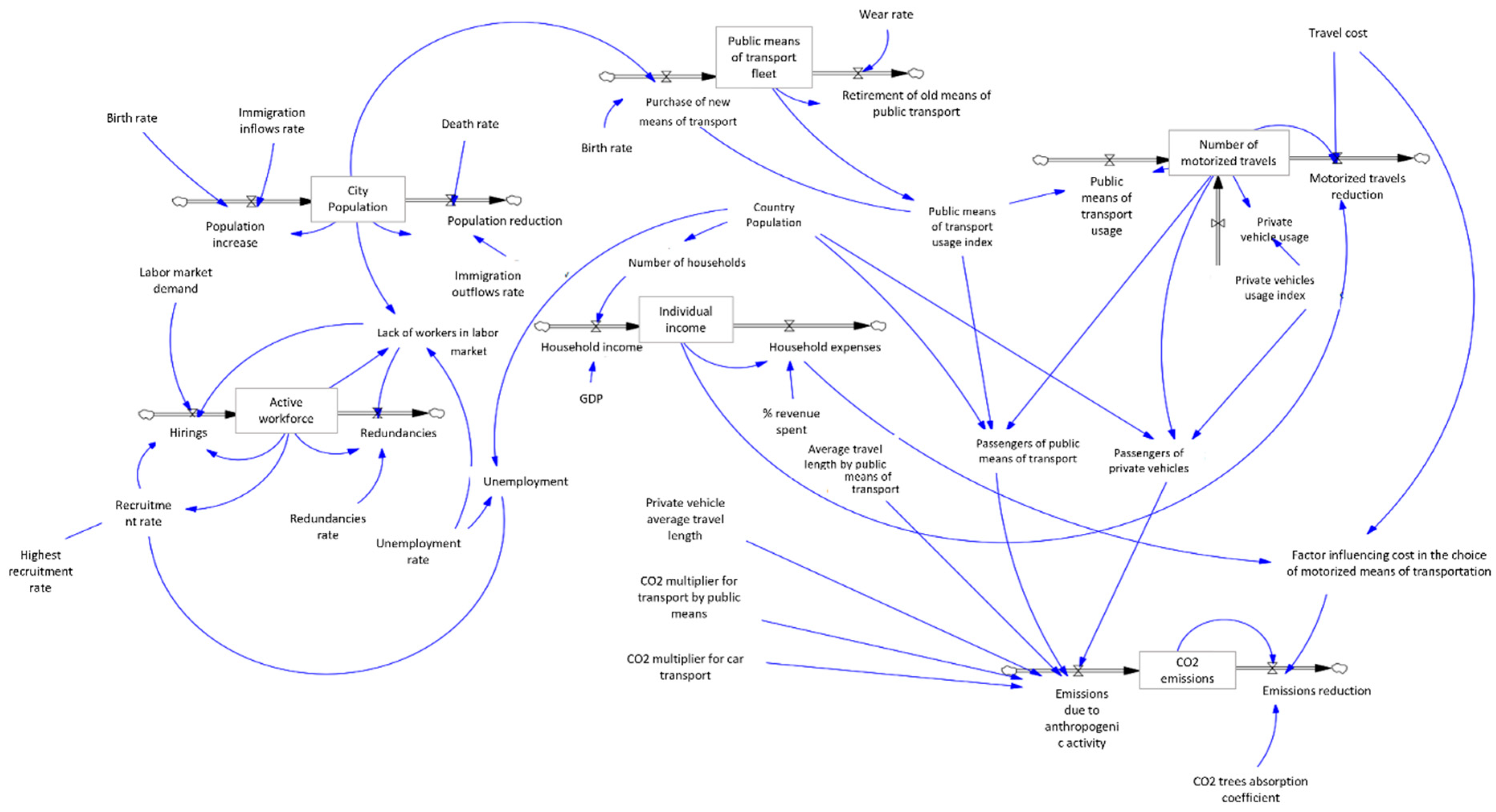
Figure 6.
Population growth over 50 years for the baseline scenario.
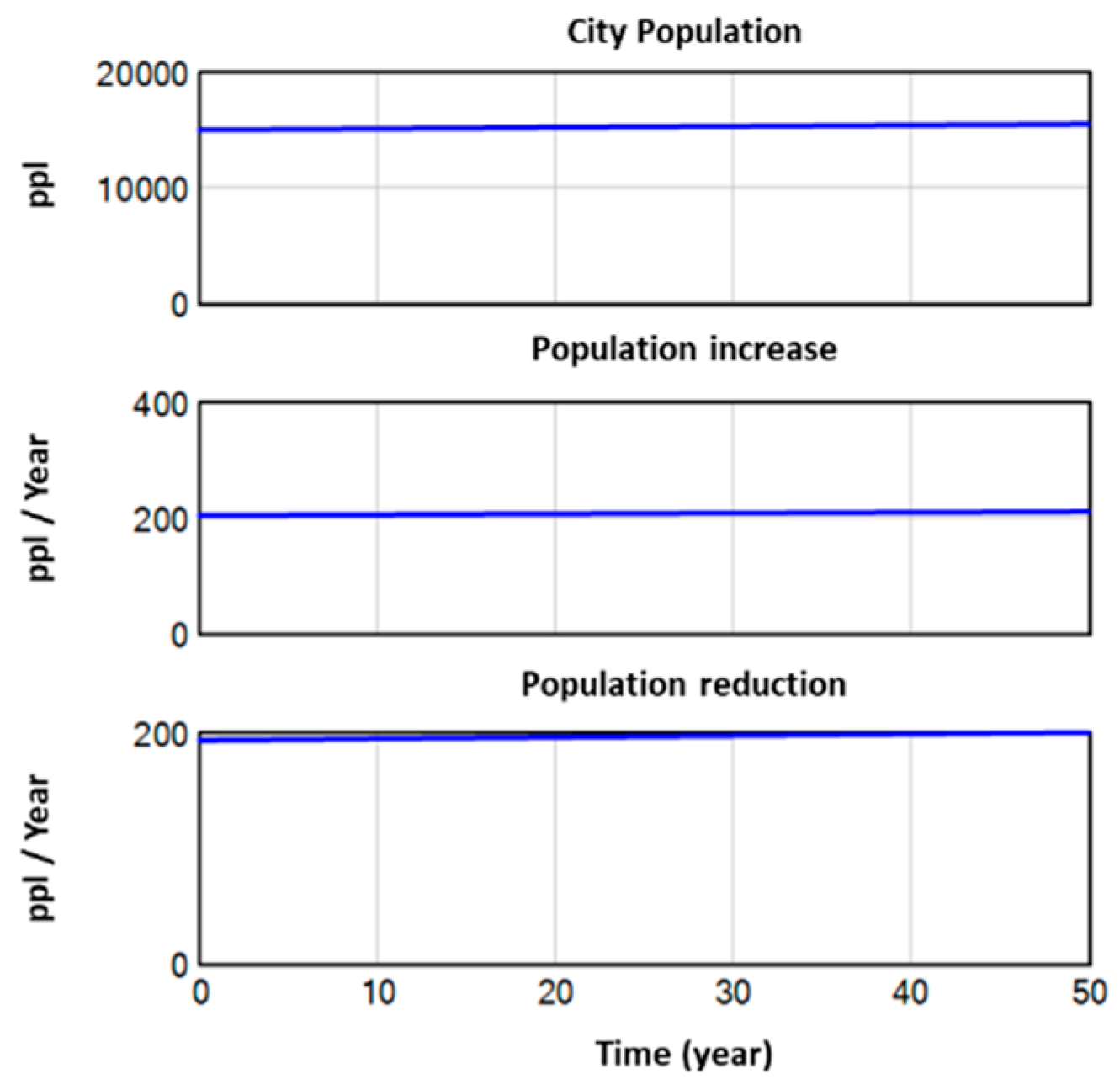
Figure 7.
Public transport fleet change within the study period of the baseline scenario.
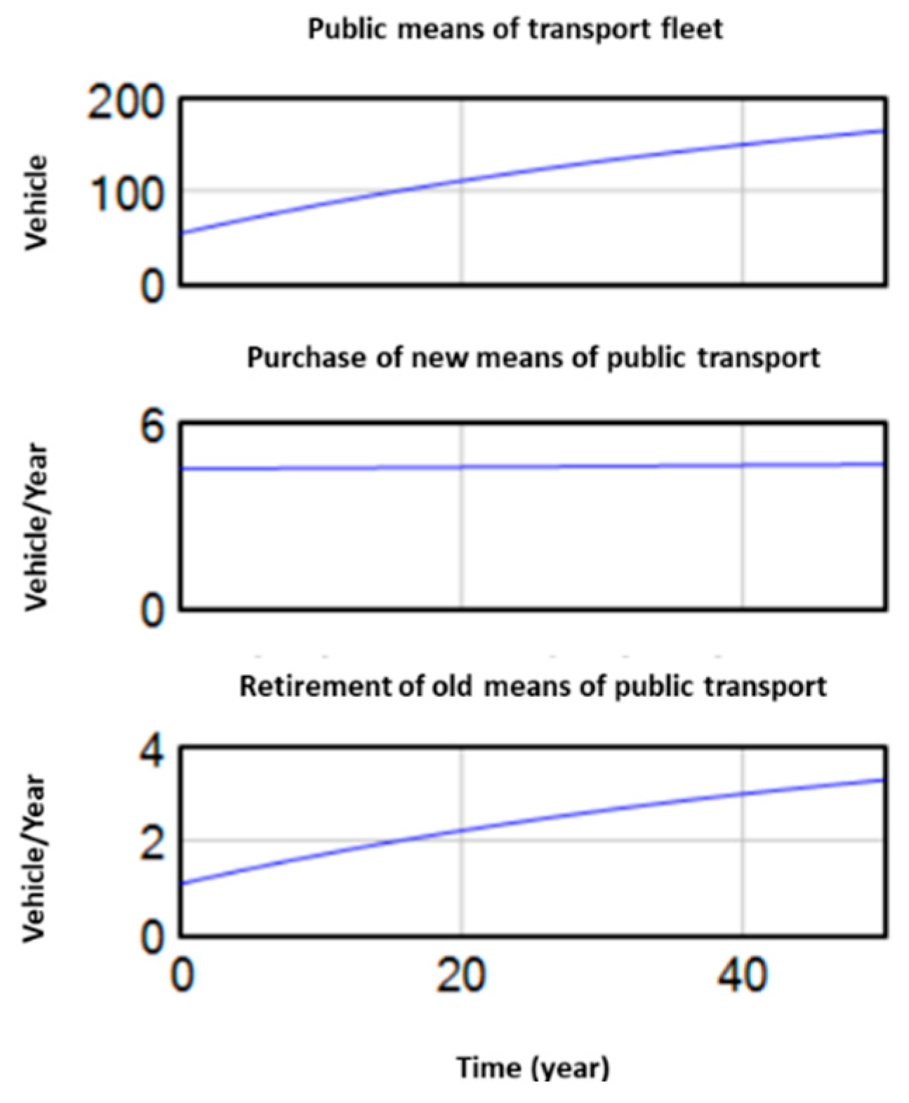
Figure 8.
Workforce change within the study period of the baseline scenario.
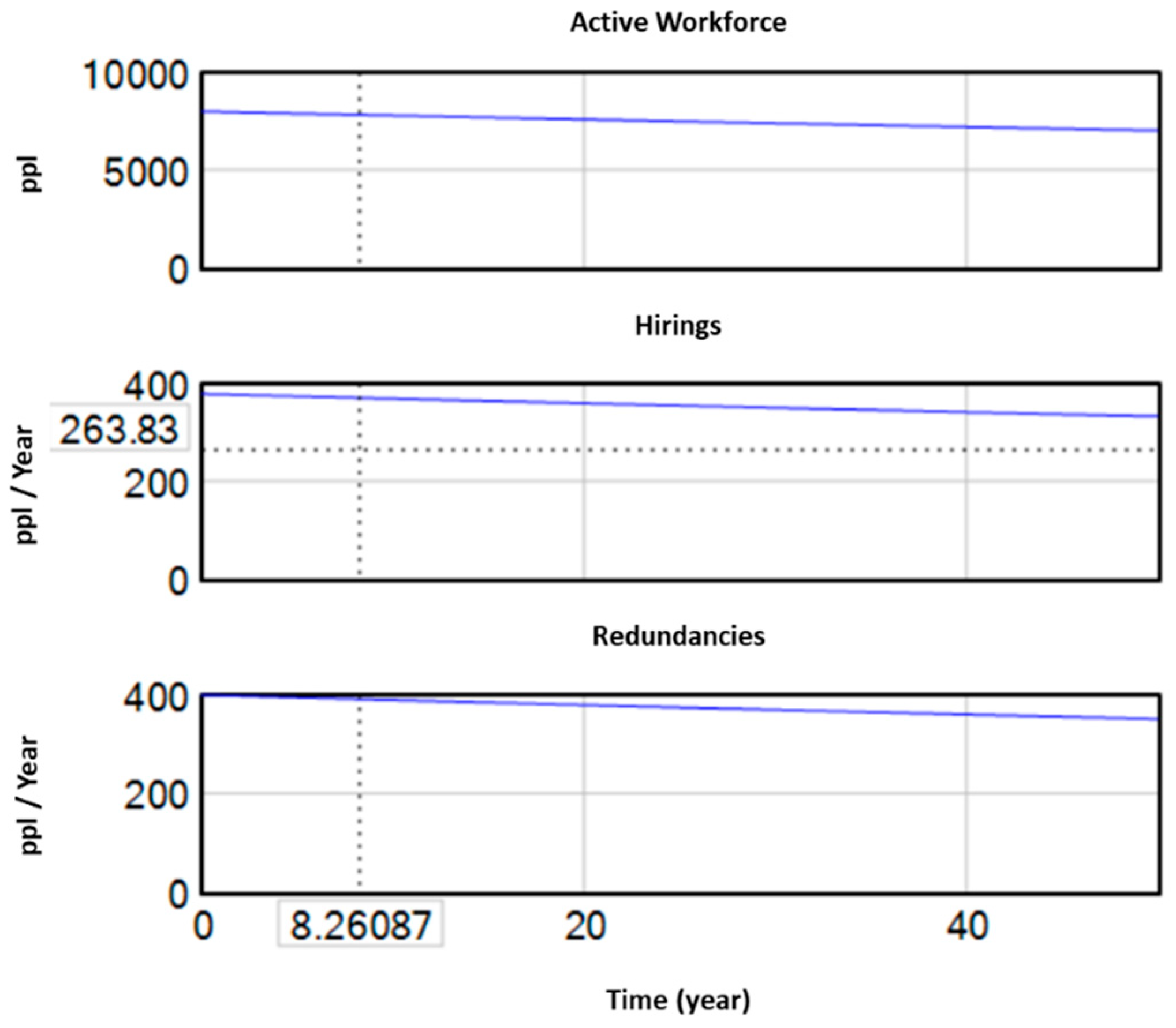
Figure 9.
Individual income and related variables change over 50 years for the baseline scenario.
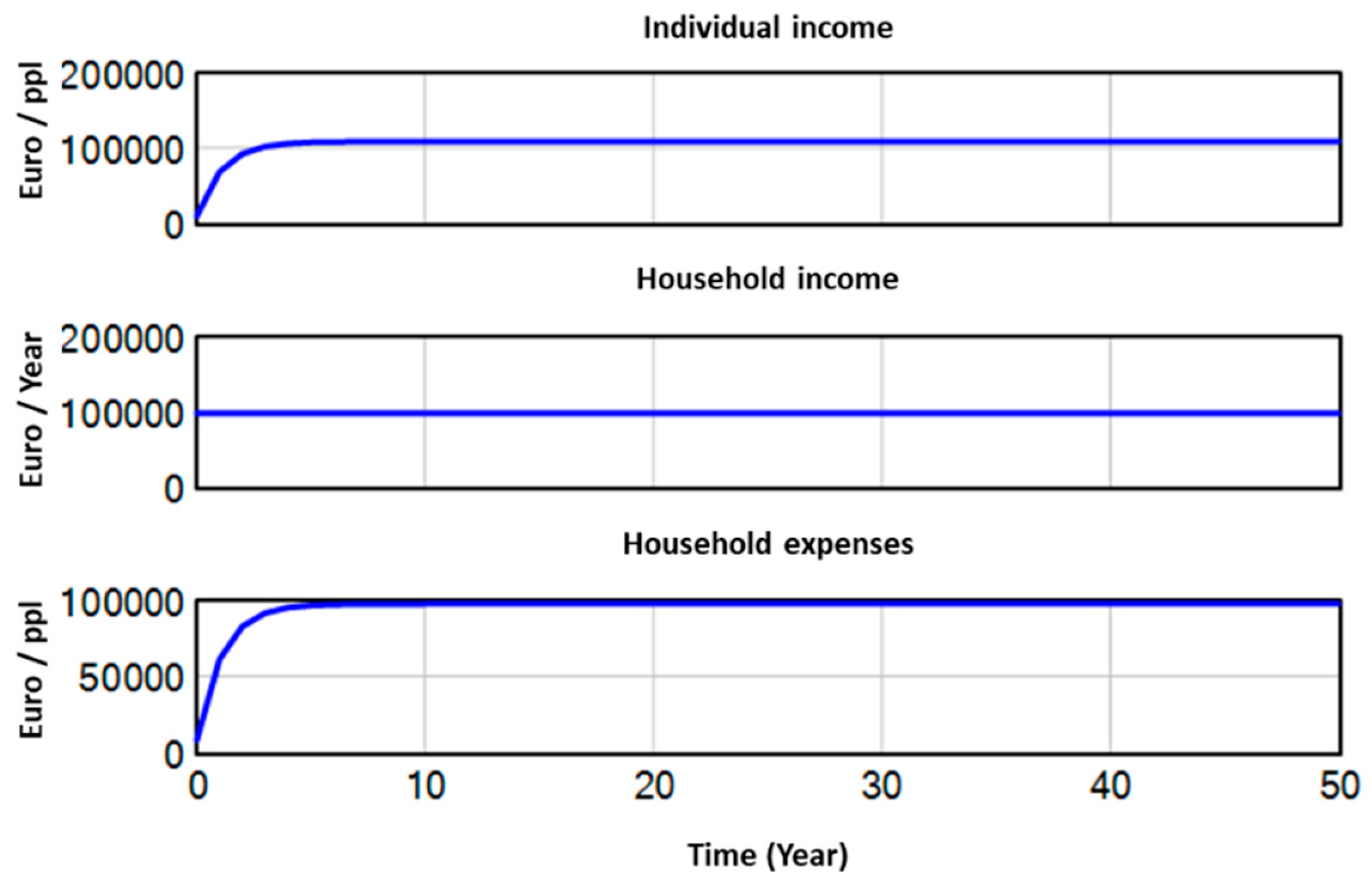
Figure 10.
CO2 emissions and related variables change over 50 years for the baseline scenario.
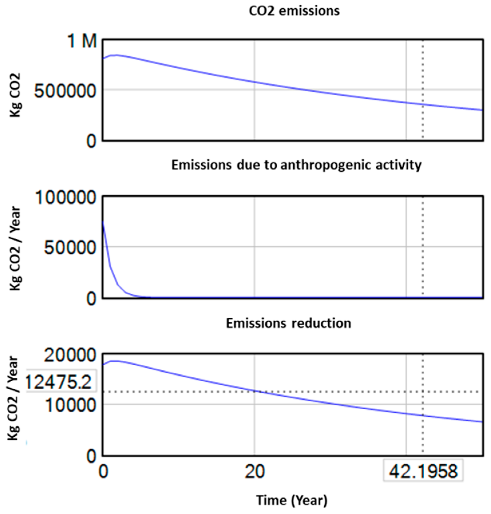
Figure 11.
Number of motorized travels and related variables change over 50 years for the baseline scenario.
Figure 11.
Number of motorized travels and related variables change over 50 years for the baseline scenario.
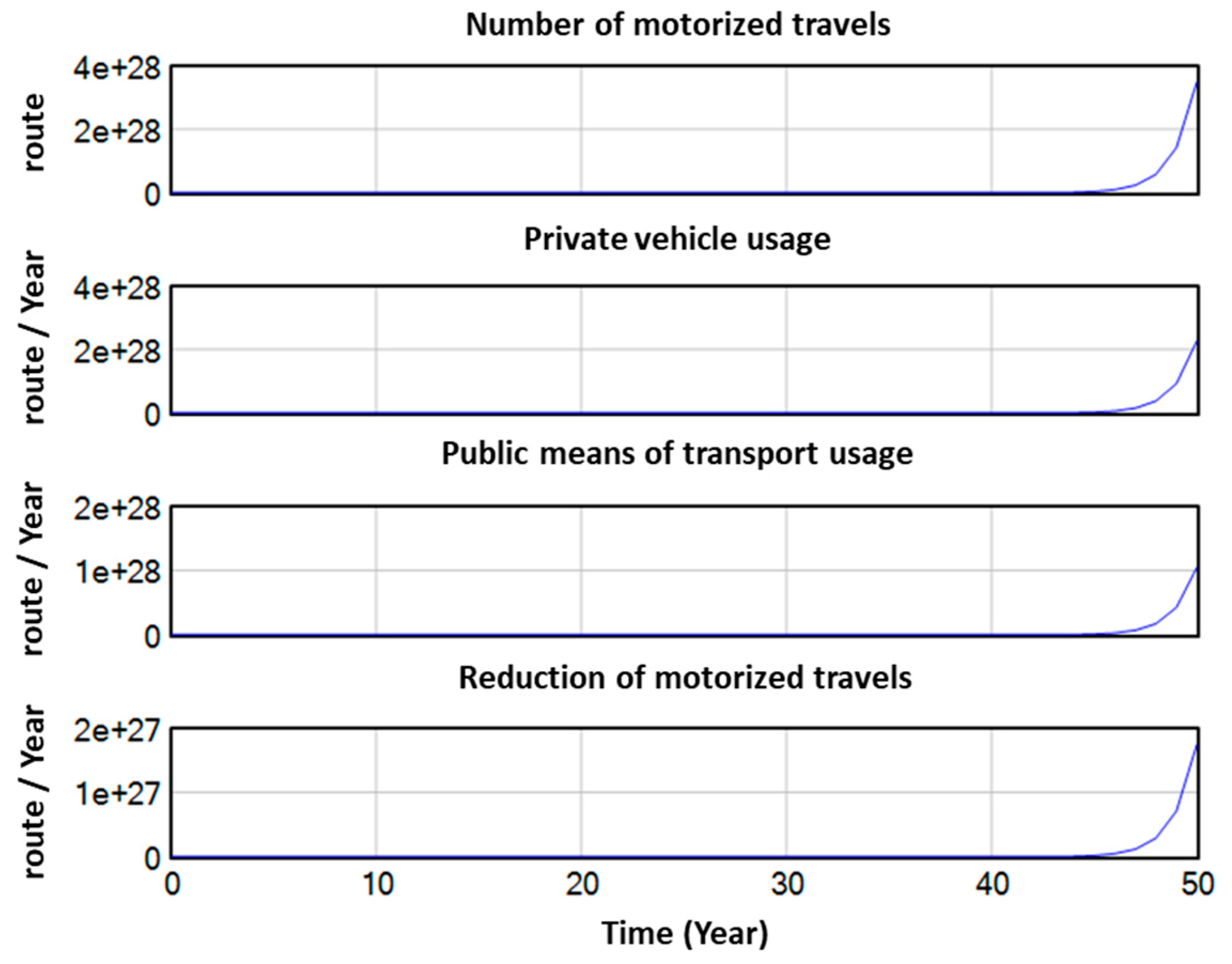
Figure 12.
Stock–flow representation of the urban system under Scenario 1.
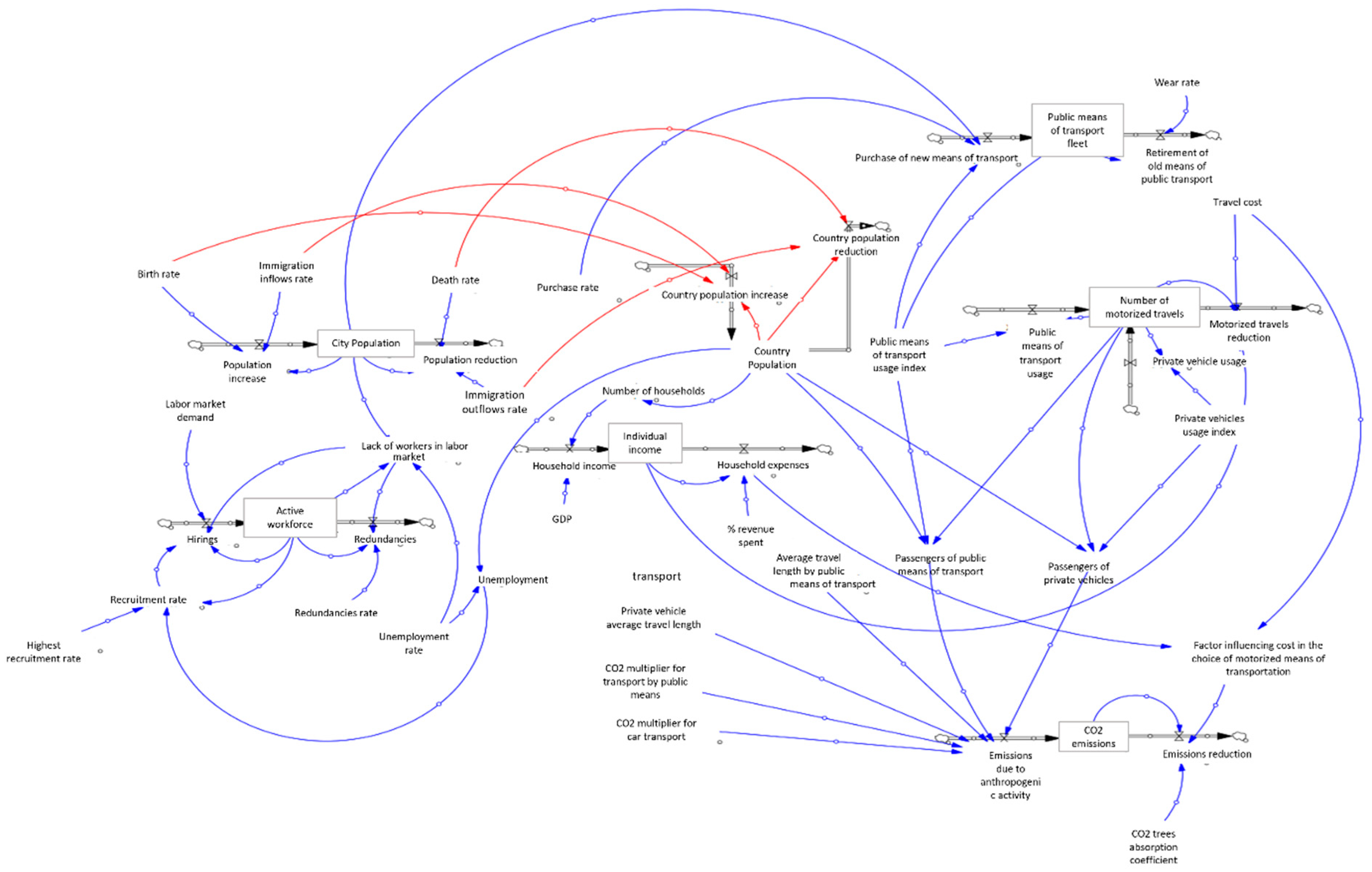
Figure 14.
CO2 emissions and related variables change over 50 years for Scenario 2.
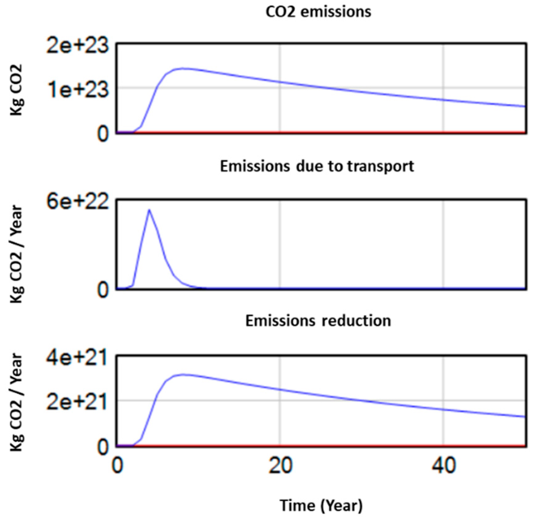
Figure 15.
Plots for all variables of interest in Scenario 3.
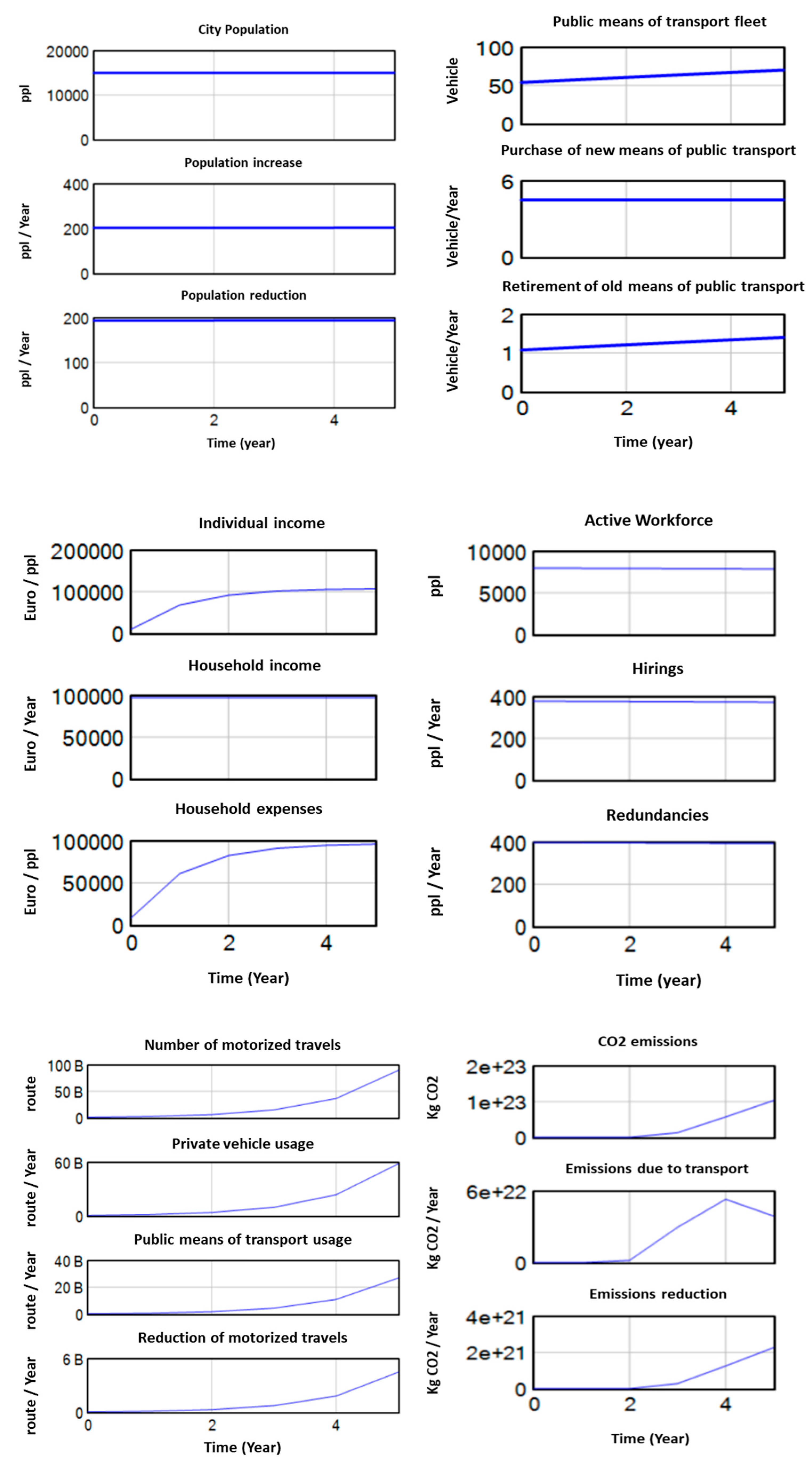

Table 1.
Description of the urban environment subsystems.
| Subsystem | Description |
|---|---|
| Society | It estimates the total population of the city, which was chosen as a “stock” variable, while the birth rate, the death rate, and the immigration rates are auxiliary variables. It is a key cluster in all models related to systems of this range, which is why it was not mentioned in the pillars to be studied. |
| Economy | It estimates per capita Gross Domestic Product (GDP) using population growth data. Variations in GDP per person can strongly influence the transportation network, as these two subsystems are connected through the economic activity generated by transport. |
| Transportation | It estimates the number of travels in the urban environment by taking into account factors such as the mode of travel, the number of cars, and the average number of passengers per car, combined with GDP per capita. |
| Environment | It estimates CO2 emissions using the number of vehicles, the distance traveled per vehicle category, and the emission factors associated with each vehicle type and fuel source. |
Disclaimer/Publisher’s Note: The statements, opinions and data contained in all publications are solely those of the individual author(s) and contributor(s) and not of MDPI and/or the editor(s). MDPI and/or the editor(s) disclaim responsibility for any injury to people or property resulting from any ideas, methods, instructions or products referred to in the content. |
© 2025 by the authors. Licensee MDPI, Basel, Switzerland. This article is an open access article distributed under the terms and conditions of the Creative Commons Attribution (CC BY) license (http://creativecommons.org/licenses/by/4.0/).
Copyright: This open access article is published under a Creative Commons CC BY 4.0 license, which permit the free download, distribution, and reuse, provided that the author and preprint are cited in any reuse.


