Submitted:
11 August 2025
Posted:
12 August 2025
You are already at the latest version
Abstract
Analysis of nonlinear plasma waves, formulated and applied for ionospheric HF heat-ing experiments, indicates that Langmuir/upper hybrid waves excited by parametric instabilities can evolve into traveling solitary waves accompanied by self-induced cavitons. These cavitons were explored by using a digisonde in fast mode. An iono-gram recorded two minutes after O-mode heater activation showed two distinct bumps in the virtual height spread, located slightly below the HF reflection and upper hybrid resonance heights. These heights are slightly below the excitation regions of Langmuir/upper hybrid PDIs by an O-mode HF heater.
Keywords:
space plasmas
; nonlinear phenomena
; parametric instabilities
; solitary waves
; ionospheric hf heating
; cubic NLSE
1. Introduction
Active wave-ionosphere interaction has been a subject of extensive research for many years. This research involves transmitting high-power HF waves from ground heating facilities, such as Arecibo [1] in Puerto Rico; EISCAT [2] in Tromso, Norway; and HAARP [3] in Gakona, Alaska, to the ionosphere. These HF heaters initiate linear and nonlinear wave-plasma interactions, which help reveal the properties of ionospheric plasma [4].
To optimize this interaction, the HF waves are transmitted with right-hand (RH) circular polarization (L-mode in a downward magnetic field) at a frequency below foF2 (the maximum plasma frequency of the ionosphere). This allows the HF waves to convert to O-mode before being reflected in the F region on the bottom-side of the ionosphere. In this region, parametric instabilities [5,6] are exciting, rapidly converting the O-mode HF waves into electrostatic (ES) plasma waves. As a result, these waves energize electron plasma, enhance airglow [7,8], generate ionization layers [9,10,11,12,13], introduce anomalous heating, and form nonlinear waves. The anomalous heating can form field-aligned density ducts [14] as well as lead to a large region of spread-F [15], and plasma density enhancement [16,17,18].
UHF/VHF radars have been used to monitor HFPLs and HFILs [2,19,20,21,22], which are indicators of the parametric excitation of Langmuir and ion acoustic waves by HF heaters. This radar detects return signals that are backscattered by electron and ion plasma waves, provided they satisfy the imposed Bragg backscattering conditions. However, a limitation of backscatter UHF radar is its inability to detect magnetic field-aligned waves, such as upper and lower hybrid waves, because these waves do not meet the Bragg backscattering conditions.
In an overdense ionosphere, the O-mode heater passes through the upper hybrid resonance layer before reaching the reflection height. Theoretical work by Stenflo et al. has shown that the HF heater can parametrically excite upper hybrid instability [23,24,25]. When intense Langmuir/upper hybrid waves evolve into nonlinear waves [26], they can form periodic and solitary envelopes [27]. Solitary Langmuir/upper hybrid waves are particularly notable as they become trapped in self-induced density cavities. The feature of electrostatic solitary structures is also of research interest in space plasmas [28]. In multi-dimensional scenarios, solitons can become unstable and collapse [29,30,31,32] if their variance identities become negative [27]. Dynamical variation of the background plasma can also instigate soliton collapse [33,34].
This study explores nonlinear waves generated by Langmuir/upper hybrid parametric instabilities, with experimental observations made using a digisonde [35,36]. The presence of plasma density irregularities is indicated by the HF enhanced virtual height-spread observed around and below the HF reflection height/upper hybrid resonance region. Further analysis suggests the manifestation of density cavities due to apparent bumps in the virtual height spread [37,38].
Section 2 details the derivation of coupled nonlinear equations for low/high-frequency electrostatic plasma waves. These equations are then combined under specific conditions for high-frequency plasma waves, particularly when low-frequency responses lack carrier frequencies, leading to the formation of cavities or density irregularities. Subsequently, Section 3 focuses on the derivation and analysis of nonlinear envelope equations for Langmuir/upper hybrid waves. Section 4 presents observations from an experiment conducted on November 20, 2009, with the results being applied to substantiate the proposed theory. A comprehensive summary of this work will be provided in Section 5.
2. Derivation of Coupled Nonlinear Equations for Low-frequency and High-frequency Electrostatic Plasma Waves
The formulation of the governing equation for low-frequency plasma density perturbations, is presented. These perturbations, which include density irregularities, ion acoustic waves, and lower hybrid waves, are driven by ponderomotive forces. These forces are induced by high-frequency electrostatic electron plasma wave fields through the nonlinearity of the plasma.
In this formulation, the perturbations are considered quasi-neutral, i.e., , and collision effects are neglected. The background magnetic field is set in the negative z direction.
The continuity and momentum equations for electron (and ion (fluids are given to be
where are the electron/ion thermal speeds, are the electron density and velocity perturbations associated with the high-frequency plasma waves, are the electron/ion cyclotron frequencies, and 〈〉 operates as a mode type filter. Applying quasi-neutral assumption, (2) and (3) are combined to a one fluid equation
where is the ion acoustic speed.
With the aid of (4), the time derivative of the ion continuity equation in (1) gives
The second term on the LHS of (5) is then expressed explicitly in terms of the derivatives on the density perturbation , a detail formulation is presented in Appendix A; hence, a nonlinear equation for the low frequency plasma density perturbation , is derived to be
The LHS of (6) is a mode equation for the low-frequency plasma waves and the RHS is the ponderomotive force induced by large amplitude high-frequency electrostatic electron plasma waves, such as Langmuir waves and upper hybrid waves. Without the nonlinear coupling, i.e., setting the RHS of (6) equal to zero, it converts to a linear mode equation, which, for instance, implies that 1. gives the dispersion relation of the ion acoustic wave, and 2. for the lower hybrid wave.
Regarding the high-frequency plasma wave, only electrons respond effectively to its field. Therefore, the formulations should only involve electron fluid equations. These can then be combined into a nonlinear equation for the electrostatic electron plasma wave field.
The continuity and momentum equations and Poisson’s equation for the electron density and velocity perturbations, and the electrostatic wave field, , are given to be
where is the total electron density; the convective term in the momentum equation (8), which is relatively small, is neglected; electron response to the wave field is adiabatic.
We now combine (7) and (8), by substituting (8) into the equation from the time derivative of (7), it gives
where is the electron plasma frequency; as shown in Appendix B, the curl term on the LHS of (10) can be explicitly expressed in terms of the derivatives on ; with the aid of Poisson’s equation (9), a nonlinear equation for the high-frequency plasma wave field , is derived to be
The LHS of (11) is a mode equation for the high-frequency plasma waves and the RHS is the nonlinear feedback. Without the nonlinear effect, i.e., setting the RHS of (11) equal to zero, it converts to a linear mode equation giving the dispersion relations of high-frequency electrostatic electron plasma waves, for instance, which include 1. Langmuir wave having the dispersion equation and 2. upper hybrid wave having the dispersion equation .
3. Nonlinear Envelope Equation for High-frequency Plasma Waves
In the absence of the plasma nonlinearity, (6) and (11) simplify to the dispersion equations for low-frequency electrostatic plasma modes, which include the lower hybrid mode: , and ion acoustic mode: . They also simplify to the dispersion equations for high-frequency electrostatic plasma modes, such as the Langmuir mode: , and upper hybrid mode: .
Set , where is the carrier frequency and c.c. stands for complex conjugate; thus, the electron linear velocity and density responses to the wave field are evaluated to be
and
where the convective term and pressure term in the electron momentum equation are neglected. are related as ascribing to In Appendix C, the RHS terms of (6) are converted to the forms in terms of the derivatives of the high-frequency plasma wave field, it leads (6) to be
Because the time variation of the high-frequency wave envelope is much slower compared to its carrier, the second time derivative on the envelope will be neglected to convert (11) to a single mode type envelope equation. After removing the carrier, (11) becomes
We now study the propagation and envelope evolution of high-frequency electrostatic plasma waves in self-induced non-oscillatory (in time) plasma density irregularities, , where the temporal variation is relatively slow.
3.1. Parallel-propagating Langmuir Wave
Set , (12) and (13) reduce to be
and
We now set in (15), where is the envelope of the Langmuir wave packet, and k is the wave number of the carrier and related to the carrier frequency through the dispersion relation , then, (15) becomes
where is the group velocity of the wave packet, , and . In a moving frame at a velocity, (15.1) converts to a conventional cubic nonlinear Schrodinger equation, which is solved via to give a traveling solitary wave solution [39]:
where the amplitude is given by the initial condition. From (14), the induced caviton is given to be
3.2. Perpendicular-propagating Upper Hybrid Wave
Set , (12) and (13) become
3.2.1. For Short-scale Density Irregularities, i.e.,
(19) becomes
Applying a similar procedure by setting in (20), where is the envelope of the upper hybrid wave packet, and k is the wave number of the carrier and related to the carrier frequency through the dispersion relation , then, (20) in a moving frame at a velocity , , where , becomes
where , and . (21) has a solution like (16), except that the initial amplitude needs to be very large for a short pulse.
3.2.2. For Large-scale Density Irregularities, i.e.,
(19) becomes
Applying the same moving frame transform as case (3.2.1.), it becomes
where (23) does not have a solitary solution.
Slightly Oblique-propagating Upper Hybrid Wave, i.e.,
Set and , where are related through the dispersion relation: ; gives thus, , (12) and (13) become
and
where is applied. Like (15), (25) has a traveling solitary wave solution,
where , , and . The induced caviton is given by (14) as
4. Experimental Observations
Digisonde is an HF radar used to probe the electron density distribution in the bottomside of the ionosphere. It transmits O-mode and X-mode sounding pulses with a carrier frequency (f) swept from 1 to 10 MHz, recording sounding echoes in an ionogram.
A sounding echo represents a backscatter signal from a layer of the ionosphere. In a stable, unperturbed ionosphere, these echoes form a smooth sounding echo trace with minimal spread in an ionogram, indicating a virtual height distribution of the ionospheric plasma. This virtual height distribution is then converted to a true height distribution using an inverse ray tracing technique [35,36].
However, when an F1 layer is present in the ionosphere, a virtual height bump appears in the sounding echo trace at frequencies near foF1. The true height profile shows a density ledge (or cusp) at foF1, which retards the propagation of sounding signals with frequencies close to foF1. This suggests that digisonde could be used to indirectly explore solitons through the co-products of cavitons.
The following outlines a study that examines the effects of HF heating experiments conducted at the HAARP transmitter facility in Gakona, AK, on November 16, 2009, 21:00 to 22:36 UTC (12:00–13:36 local time) and on November 20, 2009, from 21:10 to 23:00 UTC (12:10 to 14:00 local time) [5,15,16].
During these experiments, the HAARP digisonde operated in its normal mode, radiating within a 30° (3 dB) half-cone angle. The backscattered signals were recorded as ionogram echoes [35,36], with the digisonde receiver acquiring ionograms every 30 seconds (at the minute and 30 seconds after the minute). Each recording took less than 14 seconds, and the ionograms ranged from 1.0 to 7.0 MHz.
The HF heating experiments utilized the HAARP transmitter at full power (3.6 MW), with the HF heater transmitting at directed along the geomagnetic zenith. The heater operated in 2-minute "on" and 2-minute "off" cycles. During the "on" periods, the polarization of the heating wave alternated between O-mode and X-mode. Since the Sun remained above the HAARP horizon throughout the experiment, there was no precondition on the background plasma for each O/X mode heating period.
To analyze the impact of the HF heater, we will compare an ionogram acquired the moment the O-mode heater turned off (which still displayed ionospheric effects of the HF heater) with an ionogram acquired before next O-mode heater on. The latter ionogram represents the recovered background, as the X-mode HF heater has no impact on the ionosphere. The difference between these two ionograms reveals heater-induced changes in the background plasma density and the presence of density irregularities.
In the November 16 experiments, Langmuir PDI was the primary process. Figures 1a and 1b, recorded at 21:42 and 21:43 UT, illustrate this. Figure 1a, taken two minutes after the O-mode heater was activated, shows a significant virtual height spread and a distinct virtual height "bump" below 3.2 MHz (the HF reflection height). In contrast, Figure 1b, which represents the background plasma, has minimal echo spread and very low HF wave absorption by the lower ionosphere, as indicated by the second hop echoes.
For the November 20 experiments, upper hybrid PDI was dominant, although Langmuir PDI was also present in the early stages. This is shown in Figure 2 and Figure 3. Figures 2a and 2b, recorded at 21:52 and 21:56 UT, respectively, highlight this. Figure 2a, recorded shortly after the O-mode heater was activated for two minutes, also shows a notable virtual height spread. However, it displays two distinct virtual height "bumps" below 3.2 MHz (the HF reflection height) and 2.88 MHz (the upper hybrid resonance height). Figure 2b represents background plasma.
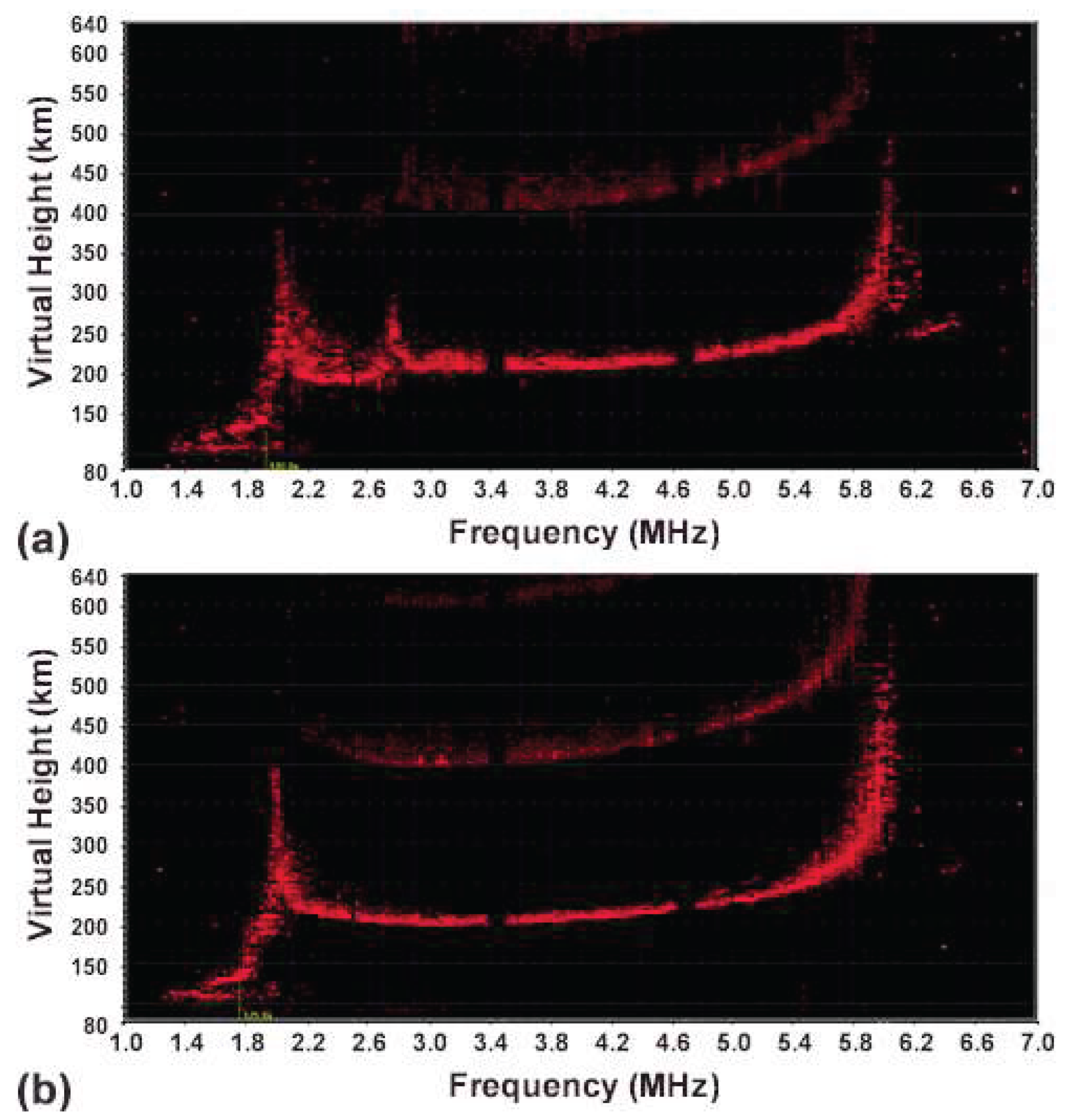
Ionograms in Figures 3a and 3b, recorded at 22:40 and 22:44 UT, respectively, show only one virtual height "bump" in Figure 3a, which appears below 2.88 MHz. Figure 3b represents the background plasma.
These heating-induced bumps are like the virtual height bump observed at foF1 when an F1 layer is present. This suggests the formation of two types of heater-stimulated plasma density cavities, located below the HF reflection height and the upper hybrid resonance height, which explain the observed bumps. These cavities are likely formed by the ponderomotive forces of Langmuir and upper hybrid waves. These plasma waves are excited by the HF heater wave through parametric instabilities in their corresponding matching regions. The November 20 experiments indicate that Langmuir PDI was suppressed by instabilities that drained heater energy in the upper hybrid resonance region.
5. Summary
Both theoretical predictions and experimental observations using UHF/VHF backscatter radars have confirmed the excitation of Langmuir PDI in HF heating experiments. While upper hybrid PDI was also theoretically predicted, it cannot be monitored by these radars. As the HF heater power increases and favorable ionospheric conditions (such as minimum D region absorption and low ionosphere) are present, the excited plasma waves intensify and nonlinearly evolve, modifying their spectral distributions.
As discussed in Section 3, these spectral waves condense into wave packages. Their envelopes are governed by a cubic nonlinear Schrödinger equation, which has traveling solitary wave solutions. Each solitary wave is accompanied by an induced caviton. This caviton forms when intense electron plasma waves nonlinearly evolve into a solitary wave, trapping it and essentially acting as a self-induced structure for pressure balance.
Naturally occurring density irregularities in the ionosphere cause the spread of virtual height echoes recorded in ionograms. When an F1 layer is present, a natural bump of virtual height echoes appears in the background ionogram near frequencies close to foF1. This bump is attributed to a density cusp at the E-F2 layer transition, which causes retardation of sounding pulses as approaches one, as well as density depletion in the cusp region. This phenomenon is demonstrated in Figure 1a.
Therefore, ionosondes can be used to detect cavitons generated in HF heating experiments, as a caviton will produce a bump of the virtual height echoes in the ionogram. Indeed, as shown in Figure 1b, two bumps of virtual height echoes appear in the HF heater modified ionogram: one slightly below the HF reflection height and another slightly below the upper hybrid resonance region. These display the cavitons associated with the Langmuir and upper hybrid solitons, respectively.
Author Contributions
original draft preparation, S.K.; all authors have read and agreed to the published version of the manuscript.
Acknowledgments
This work was supported by the US Air Force High Frequency Active Auroral Research Program (HAARP).
Abbreviations
The following abbreviations are used in this manuscript:
| HAARP | High Frequency Active Auroral Research Program |
| NLSE | Nonlinear Schrodinger Equation |
| PDI | Parametric Decay Instability |
| HF | High Frequency |
| L-mode | Left-hand Circular Polarization (with respect to the magnetic field direction) Mode |
| O-mode | Ordinary Mode |
| X-mode | Extraordinary Mode |
| HFPLs | HF Heater Enhanced Plasma Lines |
| HFILs | HF Heater Enhanced Ion Lines |
| UHF/VHF | Ultra-high Frequency/Very-high Frequency |
| RHS | Right-hand Side |
| LHS | Left-hand Side |
Appendix A: Representing the cross (second) term on the LHS of (5)
Apply the difference between (2) and (3), it gives
Substitute (A1) into (5), it yields
From (2), it gives
Because thus, (3) gives
(A3) and (A4) are combined to eliminate the terms, it gives
With the aid of the z component of (4), the time derivative of the ion continuity equation in (1) gives
which is used to represent the term in (A5); it leads to
Then,
With the aid of (A8) to represent the term in the second term on the LHS of (A2), (6) is derived.
Appendix B: Representing the cross (second) term on the LHS of (10)
With the aid of (8) and (7), the curl term in (10) becomes
With the aid of the z-components of (8), (B1) leads to
Substituting (B2) into the second time derivative of (10) and with the aid of Poisson’s equation (9), (11) is derived.
Appendix C: Evaluation of terms on the RHS of (6)
The terms on the RHS of (6) are evaluated in the following:
and
add to
and
add to
and
Hence,
References
- Gordon, W. E.; Carlson, H. C. Arecibo heating experiments. Radio Sci. 1974, 9(11), 1041-1047.
- Hagfors, T.; Kofman, W.; Kopka, H.; Stubbe, P.; Aijanen, T. Observations of enhanced plasma lines by EISCAT during heating experiments. Radio Sci. 1983, 18(6), 861-866. [CrossRef]
- Kossey, P.; Heckscher, J.; Carlson, H.; Kennedy, E. HAARP: High Frequency Active Auroral Research Program. J. Arctic Res., U. S. 1999, 1, 1.
- Kuo, S. Ionospheric modifications in high frequency heating experiments. Phys. Plasmas 2015, 22(1), 012901 (1-16).
- Kuo, S.; Snyder, A.; Lee, M. C. Experiments and theory on parametric instabilities excited in HF heating experiments at HAARP. Phys. Plasmas 2014, 21(7), 062902 (1 -10).
- Kuo, S. Plasma Physics in Active Wave Ionosphere Interaction; World Scientific, 2018; pp. 143-178. ISBN: 978-981-3232-12-9.
- Mishin, E. V.; Burke, W. J.; Pedersen, T. On the onset of HF-induced airglow at HAARP. J. Geophys. Res. 2004, 109, A02305.
- Kosch, M.; Pedersen, T.; Hughes, J.; Marshall, R.; Gerken, E.; Senior, A.; Sentman,D.; McCarrick, M.; Djuth, F. Artificial optical emissions at HAARP for pump frequencies near the third and second electron gyro-harmonic. Ann. Geophys. 2005, 23(5), 11585-1592.
- Pedersen, T.; Gustavsson,B.; Mishin, E.; MacKenzie, E.; Carlson, H. C.; Starks, M.; Mills, T. Optical ring formation and ionization production in high power HF heating experiments at HAARP. Geophys. Res. Lett. 2009, 36(18), L18107(1-4).
- Pedersen, T.; Gustavsson,B.; Mishin, E.; Kendall, E.; Mills, T.; Carlson, H. C.; Snyder, A. L. Creation of artificial ionospheric layers using high-power HF waves. Geophys. Res. Lett. 2010, 37(2), L02106(1-4).
- Pedersen, T.; Holmes, J. M.; Gustavsson, B.; Mills, T. J. Multisite Optical Imaging of Artificial Ionospheric Plasmas. IEEE Trans. Plasma Sci. 2011, 39(11), 2704-2705.
- Pedersen, T.; Mccarrick, M.; Reinisch, B.; Watkins, B.; Hamel, R.; Paznukhov, V. Production of artificial ionospheric layers by frequency sweeping near the 2nd gyroharmonic. Ann. Geophys .2011, 29(1), 47-51.
- Mishin, E.; Pedersen, T. Ionizing wave via high-power HF acceleration. Geophys. Res. Lett. 2011, 38(1), L01105(1-4).
- Blagoveshchenskaya, N.F.; Borisova, T.D.; Kalishin, A.S.; Egorov, I.M. Artificial Ducts Created via High-Power HF Radio Waves at EISCAT. Remote Sens. 2023, 15, 2300. [CrossRef]
- Kuo, S.; Snyder, A. Artificial plasma cusp generated by upper hybrid instabilities in HF heating experiments at HAARP. J. Geophys. Res. Space Physics 2013, 118(5), 2734–2743.
- Kuo, S.; Snyder, A. Observation of artificial Spread-F and large region ionization enhancement in an HF heating experiment at HAARP. Geophys. Res. Lett. 2010, 37, L07101.
- Kuo, S. Linear and nonlinear plasma processes in ionospheric HF heating. Plasma 2021, 4(1), 108-144.
- Shindin, A. V.; Sergeev, E. N.; Grach, S. M.; Milikh,G. M.; Bernhardt, P.; Siefring, C.; McCarrick, M. J.; Legostaeva, Y. K. HF-Induced Modifications of the Electron Density Profile in the Earth’s Ionosphere Using the Pump Frequencies near the Fourth Electron Gyroharmonic. Remote Sens. 2021, 13(23), 4895. [CrossRef]
- Showen, R. L. The Spectral Measurement of Plasma Lines. Radio Sci. 1979, 14(3), 503-508.
- Oyama, S.; Watkins, B. J.; Djuth, F. T.; Kosch, M. J.; Bernhardt, P. A.; Heinselman, C. J. Persistent enhancement of the HF pump-induced plasma line measured with a UHF diagnostic radar at HAARP. J. Geophys. Res. 2006, 111, A06309.
- Watkins, B. J.; Kuo, S.; Secan, J.; Fallen, C. Ionospheric HF heating experiment with Frequency ramping-up sweep: approach for artificial ionization layer Generation. J. Geophys. Res. Space Phys. 2020, 125(3), e2019JA027669 (1-12).
- Watkins, B. J.; Kuo, S. Experimental determination of threshold powers for the onset of HF-enhanced plasma lines and artificial ionization in the lower F-region ionosphere. IEEE Trans. Plasma Sci. 2020, 48(9), 2971-2976.
- Stenflo, L. Parametric excitation of collisional modes in the high‐latitude ionosphere. J. Geophys. Res. 1985, 90, 5355.
- Dysthe, K. B.; Mjolhus, E.; Pecseli, H. L.; Stenflo, L. Nonlinear electrostatic wave equations for magnetized plasmas. II. Plasma Phys. Contr. Fusion 1985, 27(4), 501-508.
- Stenflo, L.; Shukla, P. K. Filamentation instability of electron and ion cyclotron waves in the ionosphere. J. Geophys. Res. 1988, 93, 4115.
- Kuo, S. On the nonlinear plasma waves in the high-frequency (HF) wave heating of the ionosphere. IEEE Trans. Plasma Sci. 2014, 42(4), 1000-1005.
- Kuo, S. Linear and Nonlinear Wave Propagation; World Scientific, 2021; pp. 124-129 and 161-162. ISBN: 978-981-12-3163-6.
- Lakhina, G. S.; Singh, S.; Rubia R.; Devanandhan, S. Electrostatic Solitary Structures in Space Plasmas: Soliton Perspective. Plasma 2021, 4(4), 681-731; doi:10.3390/plasma4040035.
- Zakharov, V. E. Collapse of Langmuir waves. Zh. Eksp. Teor. Fiz. 1972, 62, 1745-1759; Soviet Phys. JETP 1972, 35 (5), 908-914.
- Kaufman, A. N.; Stenflo, L. Upper-Hybrid solitons. Phys. Scr. 1975, 11(5), 269.
- Stenflo, L. Upper-Hybrid Wave Collapse. Phys. Rev. Lett. 1982, 48(20), 1441.
- Stenflo, L. Wave collapse in the lower part of the ionosphere. J. Plasma Phys. 1991, 45, 355.
- Abdelrahman, M. A. E.; El-Shewy, E. K.; Omar, Y.; Abdo, N. F. Modulations of Collapsing Stochastic Modified NLSE Structures. Mathematics 2023, 11(20), 4330. [CrossRef]
- Escorcia, J. M.; Suazo, E. On Blow-Up and Explicit Soliton Solutions for Coupled Variable Coefficient Nonlinear Schrödinger Equations. Mathematics 2024, 12(17), 2694. [CrossRef]
- Reinisch, B. W.; Galkin, I. A.; Khmyrov, G. M.; Kozlov, A. V.; Lisysyan, I. A.; Bibl, K.; Cheney, G.; Kitrosser, D.; Stelmash, S.; Roche, K.; Luo, Y.; Paznukhov, V. V.; Hamel, R. New digisonde for research and monitoring applications. Radio Sci. 2009, 44, RS0A24.
- Galkin, I. A.; Khmyrov, G. M.; Reinisch, B. W.; McElroy, J. The SAOXML 5: New format for ionogram-derived data. Radio Sounding and Plasma Physics, AIP Conf. Proc. 2008, 974, 160-166.
- Kuo, S. Nonlinear upper hybrid waves and the induced density irregularities. Phys. Plasmas 2015, 22(9), 082904.
- Kuo, S. P.; Brenton, W. Nonlinear upper hybrid waves generated in ionospheric HF heating experiments at HAARP. IEEE Trans. Plasma Sci. 2019, 47(12), 5334-5338.
- Kuo, S. Nonlinear Waves and Inverse Scattering Transform; World Scientific, 2023; pp. 21-24. ISBN: 978-1-80061-405-1.
Figure 1.
Two contrasting ionograms, acquired at 21:42 and 21:43 UT from Nov. 16 experiments, show the impact of the O-mode HF heater on the ionosphere. (a) recorded at the moment the O mode heater turns off after being on for 2 minutes, and (b) recorded after the O mode heater turns off for 60s, which is an ionogram of the recovered background.
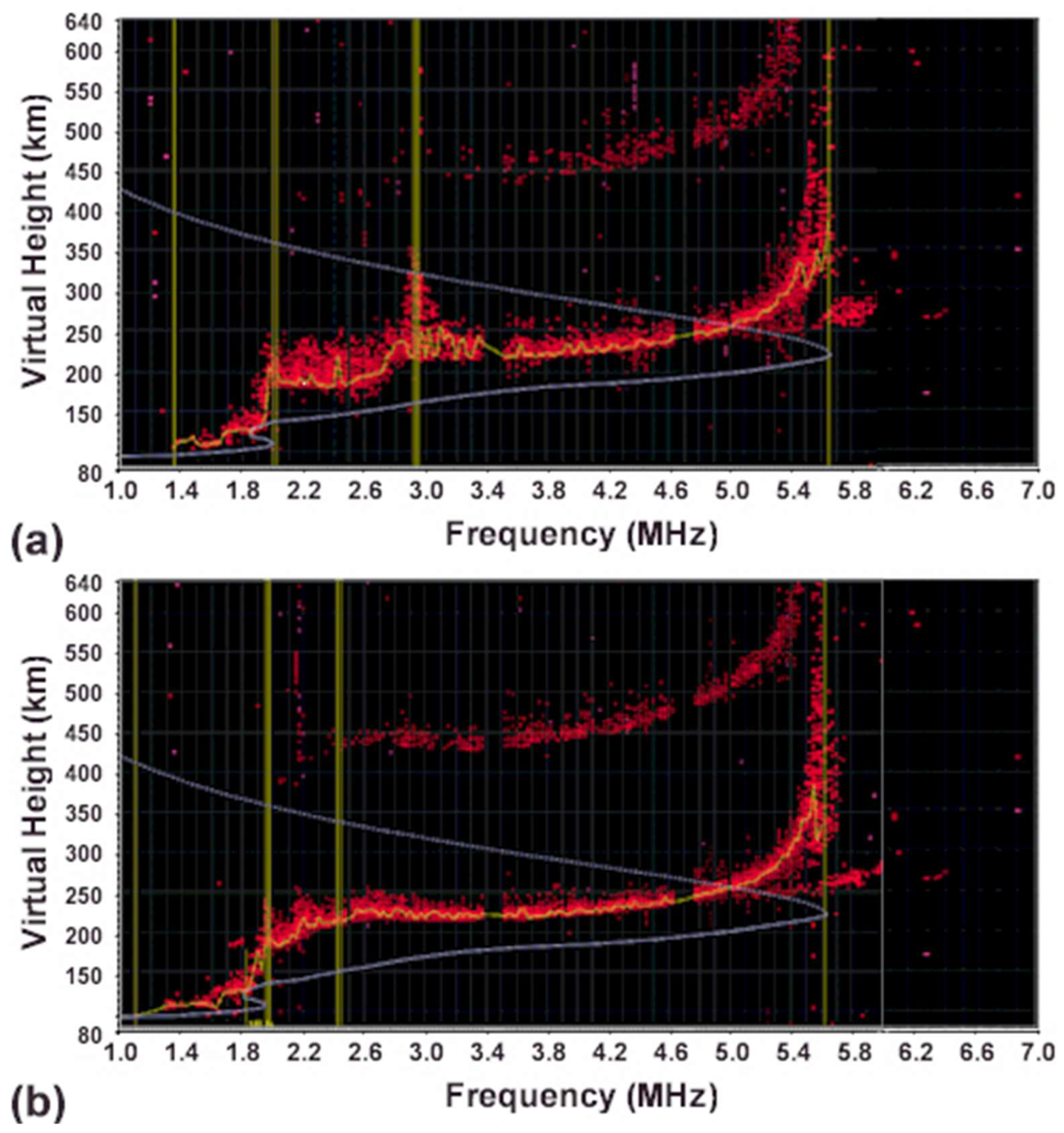
Figure 2.
Two contrasting ionograms, acquired at 21:52 and 21:56 UT from Nov. 20 experiments, show (a) the impact of the O-mode HF heater on the ionosphere and (b) the recovered background.
Figure 2.
Two contrasting ionograms, acquired at 21:52 and 21:56 UT from Nov. 20 experiments, show (a) the impact of the O-mode HF heater on the ionosphere and (b) the recovered background.
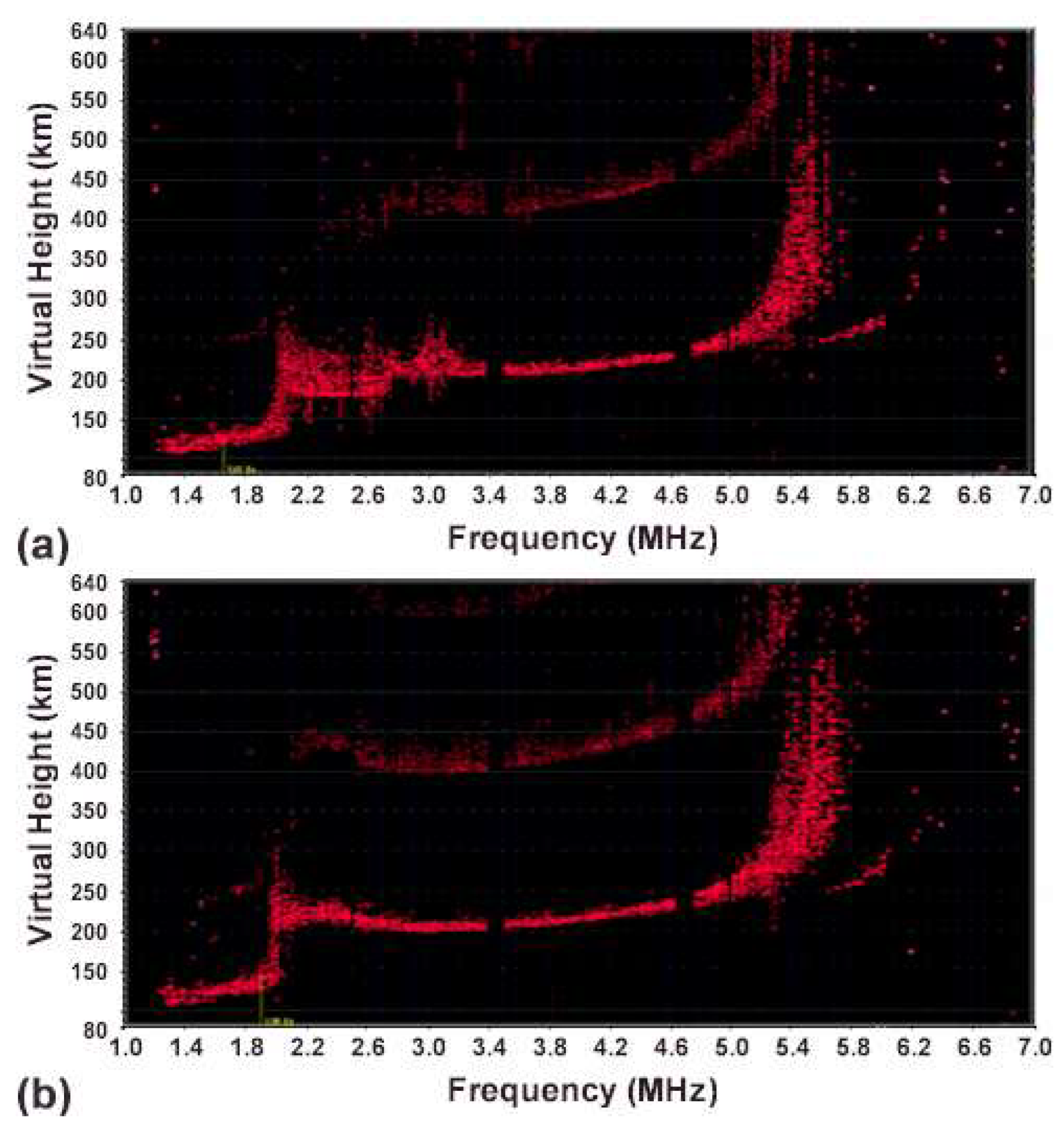
Figure 3.
Two contrasting ionograms, acquired at 22:40 and 22:44 UT from Nov. 20 experiments, show (a) the impact of the O-mode HF heater on the ionosphere and (b) the recovered background.
Figure 3.
Two contrasting ionograms, acquired at 22:40 and 22:44 UT from Nov. 20 experiments, show (a) the impact of the O-mode HF heater on the ionosphere and (b) the recovered background.
Disclaimer/Publisher’s Note: The statements, opinions and data contained in all publications are solely those of the individual author(s) and contributor(s) and not of MDPI and/or the editor(s). MDPI and/or the editor(s) disclaim responsibility for any injury to people or property resulting from any ideas, methods, instructions or products referred to in the content. |
© 2025 by the authors. Licensee MDPI, Basel, Switzerland. This article is an open access article distributed under the terms and conditions of the Creative Commons Attribution (CC BY) license (http://creativecommons.org/licenses/by/4.0/).
Copyright: This open access article is published under a Creative Commons CC BY 4.0 license, which permit the free download, distribution, and reuse, provided that the author and preprint are cited in any reuse.


