
Submitted:
08 August 2025
Posted:
13 August 2025
You are already at the latest version
Abstract
A Universal Numerical Integrator (UNI) is a computational framework that combines a classical numerical integration method, such as Euler, Runge-Kutta, or Adams-Bashforth, with a universal approximator of functions, such as a feed-forward neural network (including MLP, SVM, RBF, among others) or a fuzzy inference system. The Euler-Type Universal Numerical Integrator (E-TUNI) is a particular case of UNI based on the first-order Euler integrator and is designed to model nonlinear dynamic systems observed in real-world scenarios accurately. The UNI framework can be organized into three primary methodologies: the NARMAX model (Nonlinear AutoRegressive Moving Average with eXogenous input), the mean derivatives approach (which characterizes E-TUNI), and the instantaneous derivatives approach. The E-TUNI methodology relies exclusively on mean derivative functions, distinguishing it from techniques that employ instantaneous derivatives. Although it is based on a first-order scheme, the E-TUNI achieves an accuracy level comparable to that of higher-order integrators. This performance is made possible by the incorporation of a neural network acting as a universal approximator, which significantly reduces the approximation error. This article provides a comprehensive overview of the E-TUNI methodology, focusing on its application to the modeling of nonlinear autonomous dynamic systems and its use in predictive control. Several computational experiments are presented to illustrate and validate the effectiveness of the proposed method.
Keywords:
Adams-Bashforth neural network
; Euler-type universal numerical integrator
; neural differential equation
; Runge-Kutta neural network
; universal numerical integrator
1. Introduction
One of the first works on artificial neural networks is credited to McCulloch and Pitts in [1] and is a work from 1943. In these eighty years of development of artificial intelligence and artificial neural networks, many interesting things have emerged in this area of human knowledge. In [2], a 1957 work credited to the great Russian mathematician Kolmogorov, it is demonstrated that any n-dimensional function can be represented by linearly combining one-dimensional non-linear functions. In [3], Kolmogorov’s work from 1957 was extensively recognized, and the term Kolmogorov neural networks was introduced in the literature. In [4], the classic back-propagation algorithm is proposed for training Multi-Layer Perceptron (MLP) networks with at least one inner layer. In [5,6], it is demonstrated, independently, that MLP networks are universal approximators of functions. A very detailed summary of the main scientific knowledge achieved by artificial neural networks in the 20th century can be found at [7].
One of the great applications of artificial neural networks is in the modeling of non-linear dynamic systems in the real world. Thus, next, a bibliographical review is reported, only on this theme, considering only neural networks with feed-forward architecture trained through supervised learning.
In [8], the concept of Universal Numerical Integrator (UNI) is defined. A UNI is nothing more than the coupling of a conventional numerical integrator (e.g., Euler, Runge-Kutta, predictive-corrector, among others) with a universal approximator of functions (e.g., MLP, SVM, RBF, and wavelet networks, fuzzy inference system, paraconsistent inference system, among others). However, it is essential to note that this definition only took into account neural networks with feed-forward architecture trained exclusively through supervised learning using input/output training patterns.
Also in [8], an interesting classification for UNIs is given. According to this reference, the UNIs can be divided into three large classes, thus giving rise to three distinct methodologies, namely: (i) the NARMAX model, (ii) the mean derivative methodology (e.g., E-TUNI), and ( iii) the instantaneous derivatives methodology (e.g., Runge-Kutta neural network, Adams-Bashforth neural network, predictive-corrector neural network, among others). In [8], these methodologies are also presented in some depth, and a detailed table comparing these three methodologies is presented. It is important to note that in the classification of UNIs, the NARMAX model was included. The reason for this is that, although in the NARMAX model, the neural network is not included in the numerical integrator structure, the neural network behaves as if it were a numerical integrator.
In [9,10,11], they are all classic 20th-century books on conventional numerical integrators. The term "conventional" is used here to inform the reader that such structures do not have a universal approximator of functions coupled to them. In [12,13], the NARMAX methodology is discussed in detail using artificial neural networks. In [14] is Leonard Euler’s original work on the first-order integrator that bears his name. This is a 1768 work and initially uses instantaneous derivatives rather than mean derivatives. Everyone knows that the first-order Euler integrator, although mathematically quite simple, is relatively imprecise. However, when the instantaneous derivative functions are exchanged for the mean derivative functions, the Euler integrator becomes as accurate as any other higher-order integrator. In this case, such structures are given the special name of Euler-Type Universal Numerical Integrator (E-TUNI).
Furthermore, a correction must be given here. In [8], the E-TUNI is called Euler Neural Networks and is a 2019 reference. However, in the 2009 reference [15], the term Euler Neural Network is also used, but in a different context. Therefore, to avoid any confusion, we decided to name the first-order UNI of E-TUNI. That said, the references [16,17,18] refer directly or indirectly to E-TUNI. However, since reference [16] is relatively old, the term E-TUNI is referred to there only as Euler Neural Integrator or Mean Derivative Methodology.
In [16], the E-TUNI was coupled to a neural network with an MLP architecture and applied in a predictive control structure. In [17], a qualitative analysis on the design of a Universal Numerical Integrator (UNI) is carried out in detail. In this reference, the E-TUNI is compared with the NARMAX Model and the Runge-Kutta Neural Network (RKNN). Reference [18] is a continuation of reference [17]. In reference [18], a quantitative analysis of the design of a universal numerical integrator is presented in some mathematical depth. In [19], an important work is done involving E-TUNI in a backward integration process. It is worth noticing that E-TUNI, as well as the NARMAX model, are dynamic models that are naturally discrete and not continuous.
The first work we find in the UNI literature is credited to Wang and Lin in [20]. This reference is from 1998, and nothing before that has been found in the literature. This work is about the Runge-Kutta Neural Network (RKNN). In [21], the Runge-Kutta neural network is used in control. It is interesting to note that there is a gap of more than 20 years between the [20] and [21] references. It is also essential to note that the Predictive-Corrector Neural Network (PCNN) still does not exist in the literature. In [22], it is an essential and current work on neural differential equations. In [23], it is another work on the Runge-Kutta neural network applied in control.
It is vital to know that both the NARMAX model and the mean derivatives methodology (E-TUNI) are inherently of fixed integration step . This property means that if it is desired to change the integration step in these two methodologies, then it is necessary to do a new neural training. However, in the instantaneous derivatives methodology (RKNN, ABNN, PCNN, among others) the integration step can be changed, within certain limits imposed by the order of the referred integrator used, without having to carry out a new training [8,17,18,20]. Finally, some small theoretical models of non-linear ordinary differential equations can be taken from [24] to test any UNI.
The original contributions of this paper are as follows: (i) it presents an overview of how E-TUNI works to solve dynamics and control problems, (ii) it presents three studies of practical technological applications of the proposed model (e.g., including the orbit transfer problem and the non-linear simple pendulum problem), (iii) it presents a practical example of how to generate an approximate continuous solution for the E-TUNI model (see the nonlinear simple pendulum problem), which is naturally discrete in solution, and (iv) it presents a correct proof of the general expression for E-TUNI, since in [16] it is not correct. Furthermore, the E-TUNI has its origins in [16].
Accordingly, the remainder of this article is organized as follows. Section 2 describes in detail the meaning of the main discrete and continuous variables, which are used to describe the proposed E-TUNI model. Section 3 presents a concise yet comprehensive theoretical overview of the Euler-Type Universal Numerical Integrator (E-TUNI), outlining its foundational principles and key mathematical formulations. Section 4 details three numerical simulations that serve to validate the proposed methodology and demonstrate its practical effectiveness. Finally, Section 5 summarizes the main conclusions, highlighting the contributions and potential future directions of this research.
2. Preliminaries and Symbols Used
To facilitate a deeper understanding of the theoretical framework developed in this paper, we present a complete definition of all symbols and variables used throughout the work. The proposed methodology is named Euler Type Universal Numerical Integrator (E TUNI), and it is based on a forward integration scheme that operates in a discrete-time setting. This approach is designed to approximate the behavior of continuous-time autonomous ordinary differential equations by means of a discrete formulation. For clarity, all notation used in this context is listed below and classified into two main categories: (i) variables defined in continuous time and (ii) variables defined in discrete time.
(i) Continuous Variables
- … System of continuous differential equations.
- … State Variables.
- … Instantaneous derivative functions.
- … Particular continuous and differentiable curve of a family of solution curves of the dynamical system .
- … First derivative of .
(ii) Discrete Variables
- … Vector of state variables at time .
- … Scalar state variable for at time . It is a generic discretization point of the state variables generated by the integers i, j, and k.
- n… Total number of state variables.
- … Vector of control variables at time .
- … Scalar control variable for at time .
- m… Total number of control variables.
- … Exact vector of state variables at time .
- … Exact scalar state variable for at time .
- … Estimated Vector of state variables by UNI or E-TUNI at time .
- … Scalar state variable estimated by UNI or E-TUNI for at time .
- … Estimated Vector of state variables when using only the integrator and without using the neural network at time .
- … Exact vector of positive mean derivative functions at time .
- … Scalar positive mean derivative functions for at time .
- … Estimated vector of positive mean derivative functions by the E-TUNI at time .
- … Vector of positive instantaneous derivatives at time .
- … Scalar positive instantaneous derivative for at instant .
- … Time instant .
- … Time instant .
- … Integration step.
- i… Over-index that enumerates a particular curve from the family of curves of the dynamical system to be modelled ().
- j… Under-index that enumerates the state and control variables.
- k… Over-index that enumerates the discrete time instants ().
- r… Total number of horizons of the time variable.
- q… Total number of curves from the family of curves curves of the dynamic system to be modelled.
- … Instant of time within the interval as a result of the Differential Mean Value Theorem (see Theorem 1).
- … Instant of time within the interval as a result of the Integral Mean Value Theorem (see Theorem 2).
To interpret the notation used in this work, it is essential to distinguish between the variables , , and . The vector variable is the exact value of the state variables at time . The vector variable is the estimated value of the state variables using only the numerical integrator. Finally, the vector variable is the estimated value of the state variables using the numerical integrator coupled to an artificial neural network. Figure 1 follows this convention and helps to understand better the notations adopted here. Additionally, it is important to understand the meaning of the auxiliary variables i, j, and k. This is accomplished in the next paragraph.
A key point in this notation is the interpretation of the over-indexes k and i and the under-index j in the variables and . When the auxiliary variables i, j, and k are used simultaneously, they uniquely identify the secant () at the point . Note that the over-index k indicates the time instant of the secant, the under-index j indicates the state variable in question, where , and the over-index i indicates the particular curve where the respective secant is located, from the family of possible curves of the system of differential equations considered. The value of q can be as large as desired. The larger the value of q, the more different curves the neural network trains on, and the better its generalization. This convention is quite useful to fully understand the formal proof of the general expression of E-TUNI that is performed in section 3.2.
3. Mathematical Development
In this section, we present a concise and complete description of the Euler-Type Universal Numerical Integrator (E-TUNI). To this end, we present a formal mathematical proof for the general expression that governs E-TUNI’s operation to generate discrete solutions for autonomous nonlinear dynamical systems governed by ordinary differential equations. Additionally, we also present the correct way to use E-TUNI in a predictive control framework. We conclude this section by obtaining an approximate mathematical expression for E-TUNI to provide a continuous solution, rather than a discrete solution, for autonomous dynamical systems.
3.1. Basic Mathematical Development of E-TUNI
We provide a brief mathematical description of E-TUNI below. Then, in the following sub-section, we perform a formal mathematical demonstration of the general expression of the first-order Euler Integrator designed with mean derivative functions. So, by definition, the secants or mean derivatives for between the points and are given by:
where, is the forward state of the dynamic system, is the present state of the dynamical system, the over-index k on the left indicates the instant k, the over-index i on the right suggests a discretization of the continuum, the sub-index j on the right indicates the j-th state variable, n is the total number of state variables and is the integration step. We talk more about the over-index i later in this article.
A geometric and intuitive difference between the mean and the instantaneous derivative functions is shown in Figure 1. In line with the Figure 1 and Figure 2, the E-TUNI is entirely based on the concept of mean derivative functions and not on the idea of instantaneous derivative functions. As will be seen throughout this article, this change is quite significant when incorporated adequately into the Euler-type first-order integrator. Furthermore, the mean derivative functions can also be obtained from supervised training with input/output patterns using a neural network with any feed-forward architecture (MLP, RBF, SVM, among others).
It is also essential to note that it is possible to train E-TUNI in two different ways, namely: a) through the direct approach or b) through the indirect or empirical approach. In the direct approach, the neural network is trained decoupled from the Euler-type integrator, while in the indirect or empirical approach, the neural network is trained coupled to the structure of the first-order Euler integrator. For this reason, in the indirect approach, the back-propagation algorithm needs to be modified slightly. In the references [8,17,18] this is explained in more detail.
In this way, be a non-linear dynamic system of n simultaneous first-order equations with dependent variables . If each of these variables satisfies a given initial condition for the same value a of t, then we have an initial value problem for a first-order system, and we can write:
In [14], the mathematician Leonard Euler himself proposed in 1768 the first numerical integrator, in the history of mathematics, to approximately solve non-linear dynamical systems governed by the equation (2). This solution, which is well-known to everyone, is given by:
where, for are instantaneous derivative functions, according to the graphical notation shown in Figure 1. On the other hand, there is an attempt in [18] to prove mathematically that if you exchange the instantaneous derivatives in (3) for the mean derivatives, then the solution proposed by Leonard Euler becomes accurate, i.e.,
Comparing equations (3) and (4), it is observed that the instantaneous derivative functions do not depend on the integration step, but the mean derivative functions do. Additionally, the equations in (4) can also be expressed in a more compact notation, given by:
where, […, [… e […. The generalization of the mean derivatives methodology to multiple backward inputs and/or multiple forward outputs is relatively easy. This expression can be obtained by following the equation:
where p is the number of backward and/or forward instants and . For example, if then it is possible to design an E-TUNI with inputs in the role of backward mean derivatives and outputs in the role of forward mean derivative. In this way, the reader is free to choose the values of and as long as the previous equality is satisfied. However, it should be noted that the first input of the neural network must be an absolute value, not a relative one.
On the other hand, notice that if the reader tries to compare the NARMAX model with the E-TUNI structure, one can see that the former is very similar to the latter. In the NARMAX model, for example, the output of the universal approximator of functions is the forward instant . However, in the E-TUNI model, the output of the universal approximator of functions is the mean derivative function at the present instant. This description is the only practical difference between these two methodologies. However, the E-TUNI may be a little more computationally efficient than the NARMAX model, as explained in the following paragraph.
Considering the direct approach to training the mean derivative functions required by the E-TUNI structure, it is then possible to perform a theoretical analysis of the local error committed by this first-order universal numerical integrator. Thus, let the exact value and the estimated value be obtained, respectively, by the equations (7) and (8) of a given solution of a generic dynamical system.
where is the mean absolute error of the output variables of the universal approximator of functions used to learn the mean derivative functions. Thus, if the equation (7) is subtracted from the equation (8) and the result of this subtraction is squared, we have:
The equation (9) states that the local squared error made by E-TUNI can dampen the squared error of training the universal approximator of functions, used in neural training, if . If , the local error will be amplified. However, for a more accurate analysis of the global training error, further studies are needed.
The equation (9) is fundamental, as it partially explains why training the E-TUNI with a mean square error , greater than that obtained by training the NARMAX model can also yield good results from estimation and potentially surpass those obtained in the NARMAX methodology. However, as stated earlier, this is true only if .
Therefore, an E-TUNI neural integrator can be used for supervised training of a generic plant. Additionally, this plant can be used in a predictive control framework. Thus, the plant’s neural model can be used, as a model of the system’s internal response to derive a smooth control policy. This control is then able to track a reference trajectory by minimizing a finite-horizon quadratic functional, given by [16]:
where, is the reference trajectory at the instant ; m is the number of horizons ahead; and are positive definite weight matrices; is the output of the previously trained E-TUNI. Thus, in [16] it is shown that it is necessary to know the partial derivatives to solve the problem of optimization given by the equation iteratively (10) through the Kalman filter. Also, in [16] these partial derivatives can be calculated as follows:
where,
In the equations (11) to (14), we have that is the total number of state variables and is the total number of control variables. Furthermore, to derive these equations, it was assumed that the neural network, which learns the mean derivative functions, was designed with only one late input for the state and control variables, and also only one forward output for the mean derivatives.
So, for example, if a neural network with an MLP architecture is used, the calculation of the partial derivatives, necessary for the use of the gradient training algorithm, can be obtained as follows [16]:
where,
It is essential to note that l is a generic layer of the MLP network. So are the output values of the l layer, and when l is the last layer, then these outputs necessarily are the mean derivative functions. The functions can be any sigmoid function. Furthermore, if another neural architecture is used, for example, RBF networks or Wavelets, it will only change the equation (15). The equations (11), (12), (13) and (14) remain unchanged. The reason for this is that the equations from (11) to (14) refer exclusively to the type of integrator used, which, in this case, is necessarily the E-TUNI.
On the other hand, the equation (15) refers exclusively to the type of feed-forward neural network used, which, in this case, is necessarily the MLP network. Thus, the equation (15) is nothing more than an iterative version of the back-propagation algorithm, which calculates the partial derivatives from the output of the MLP network, concerning its inputs and not concerning the synaptic weights.
It is also worth noticing that, to fully understand the equations from (11) to (14), it is convenient to consult the reference [16], as it is necessary to make a temporal chain of several first-order Euler integrators, which work exclusively with mean derivative functions. This fact is because the horizon m has, in general, temporal advances in an amount greater than the total number of delayed inputs of the E-TUNI used.
3.2. Correct Mathematical Demonstration of the E-TUNI General Expression
In this section, we formally demonstrate the general mathematical expression of E-TUNI, which is nothing more than a first-order Euler-type integrator working with mean derivative functions. This development is done here because, as previously stated, there is a demonstration error in the general E-TUNI expression presented in reference [16]. So, the starting point is Figure 3.
So, for the reader to understand this figure, we explain it, starting from the point . The point is an instant of the solution of the considered autonomous dynamic system. The variable j means the jth state variable of the considered dynamic system, where , that is, there are a total of n state variables. The variable i represents the i-th curve of the family of curves confined in the interval and which is the solution of the considered dynamic system. By the continuum hypothesis, one can have infinite curves (). The variable k represents the k-th instant of time, that is, . In the case of the variable k, if the dynamical system solution does not come out of the region of interest [] and the system is autonomous then the variable k can also go to infinity (). Also, when we write or it means that and .
This notation for is sufficient to uniquely map it to its respective region of interest, where its associated secant characteristic is confined. So, in this case, for example, we can say that for the state we have its associated characteristic secant given by .
Thus, the secant is associated with the state variable with a curve i specific to the family of solutions, in this case, by and the instant . The fact that the secant is associated with the instant means that it is confined to the closed interval . Thus, the secant starts at and ends at .
Furthermore, the states and are special states, where both and are also confined to the closed interval . The instants as are directly associated, respectively, with the integral mean value theorem and the differential mean value theorem [25,26]. So, having made these preliminary considerations, we begin now with this demonstration in a precise manner. Thus, let the following autonomous system of non-linear differential equations be given by,
Consider also, by definition, for a particular trajectory for a family of solutions to the system of differential equations passing through at instant , i.e., initializing from a domain of interest , where and are finite. It is also appropriate to introduce the following vector notation over (16):
In [25], by definition, the secant curve between two points and belonging to the curve to is the line segment joining these two points. Thus, the tangents of the secants between the points and , and , …, and are defined as:
with,
for . Thus, we can state now the two fundamental theorems to consolidate our proof. These two theorems are the differential mean value theorem and the integral mean value theorem, which are presented below without proof [25,26].
Theorem 1 (The Differential Mean Value Theorem): If a function for is a continuous function and defined over the closed interval is differentiable over the open interval , then there is at least one number with such that,
Theorem 2 (The Integral Mean Value Theorem): If a function for is a continuous function and defined over the closed interval , then there is at least one inner point in such that,
It is important to note that generally is different from . Also, the mean value theorems say nothing about how to determine the value of and . These two theorems simply state that and are confined to the closed interval .
Property 1: Applying Theorem 2 on the curve is equivalent to applying Theorem 1 on the curve both on the same interval closed , that is, .
Proof: from Theorem 2 applied to the continuous curve results in a for such that as a result of the fundamental theorem of calculus. Thus, . On the other hand, the application of Theorem 1 about the continuous and differentiable curve implies the existence of a for , such that . Thus, . However, this proof does not prove that . □
That said, we prove now the main theorem of this section, namely Theorem 3. But before that, it is worth commenting on some preliminary considerations. In Theorem 3 when we write we are specifying that the general dynamical system is harnessed to the particular solution of the curve i belonging to the family of curves that is a solution of . Thus, is an alternative way of saying that the general dynamical system is harnessed to some initial condition . Thus, the notation with the index i is more didactic to accept the uniqueness of the mapping explained at the beginning of this sub-section in Figure 3. However, in this article, we did not prove the uniqueness of the mapping discussed in Figure 3, but we assume it is true. To better understand this type of mapping, see a practical example of the same that appears in [19] (see Fig. 7 in this same reference).
Another essential consideration for understanding the proof of Theorem 3 is that it is necessary to know the solution of the dynamic system beforehand, which can then be solved using the Euler integrator that works with mean derivative functions. Also, notice that, since we are working with supervised learning with input/output training patterns, this is not absurd. This fact is easy to understand, as it is necessary to know the references and to accurately estimate the mean derivative , between these two points, through a universal approximator of functions with exclusively feed-forward architecture.
Thus, if the solution of the non-linear dynamical system that is wanted to estimate, then it is necessary to treat this problem as n independent equations with only one time variable t each (black-box approach), rather than n vector coupled equations (white-box approach). This last statement can be justified with the help of Principle 1, which is proved, by reduction to absurdity, right after the proof of Theorem 3.
Therefore, if the solution of the considered dynamic system is previously known and given by for and then the function are easily obtained by direct differentiation (numerically or analytically). In this way, the original dynamic system can be replaced by for and , for a time interval confined in with the help of Principle 1.
However, it should be noted that the math function , in general, has nothing similar to the math function . Note also that this simplification makes it possible to reduce the proposed proof to a differential calculus of only one variable. Thus, it allows the use of the differential and integral mean value theorems. Note that must also have the over-index i, as this function must necessarily also depend on the initial condition as well as its equivalent instantaneous derivative function .
Theorem 3: The discrete and exact general solution for the autonomous system of non-linear ordinary differential equations of the type can be established through the first-order Euler relation of the type , for and fixed; since that the general solution of this dynamical system, given by, and are, previously, known for ; and t. Furthermore, the solutions for must all be continuous and differentiable. However, note that for is suffice to be continuous.
Proof: Let the autonomous non-linear dynamical system of first-order be given by for and . If the dynamical system solution is known and equals to then the function can be replaced by , that is, . In this way, we can write that . Note that the indices i, j, and k uniquely map the secant that interests us according to Figure 3. This last integral can still be simplified as as a result of the fundamental theorem of calculus. So, applying the integral mean value theorem, in this last expression, we get where and for . On the other hand, applying the differential mean value theorem on the function for in the interval we get that . So, by Property 1 we have that to . So, to or, in vector form, it turns out that
The reason that the functions for are all continuous and differentiable is that, in the proof of Theorem 3, we used the differential mean value theorem over and this theorem requires these two conditions to be applied. The reason that the functions for are all continuous is that, in the proof of the same Theorem 3, the integral mean value theorem was applied over the function and this theorem requires this condition. Note that for the application of the integral mean value theorem, the function is not required to be differentiable.
Principle 1: Given the non-linear autonomous dynamic system and their respective general solutions for and then, the autonomous instantaneous derivative functions can be replaced by the exclusively non-autonomous instantaneous derivative functions given by , that is, for and .
Proof: Assume, for absurdity, that the referred principle is false. If this is true, then there would be no compromise of veracity between the computational data acquisition system (through sensors) and the real universe, and thus the black-box approach would not work; but this is absurd. So, by exclusion, the principle is true . □
Notice that when a computational data acquisition system is performed, for example, from a particular real-world plant, something interesting happens. Thus, whoever maintains the consistency of the acquired data, through several sensors acting simultaneously and independently of each other, is the omnipresent and immutable manifestation of the natural physical laws, which govern the proper functioning of the universe (e.g., the law of universal gravitation, conservation of energy law, Faraday’s law, among others). In this case, little is allowed to human wisdom and technology.
Finally, the E-TUNI universal numerical integrator is suitable for solving only ordinary differential equations. However, it should be noted that the current use of neural networks in solving Partial Differential Equations (PDEs) is quite extensive [27,28,29,30,31,32,33,34,35]. Additionally, [36] explains how to use the Runge-Kutta numerical integrator to solve partial differential equations (mainly hyperbolic ones). Therefore, using the E-TUNI to solve partial differential equations may be a good option for future work and should be investigated more carefully.
3.3. Mathematical Relationship Between Mean and Instantaneous Derivatives
A very remarkable fact is that it is possible to obtain an equation that relates the instantaneous derivative functions to the mean derivative functions. This equation can be easily obtained using the chain rule for functions on several independent variables [25,26]. In this way, two previously trained neural networks are known to represent the instantaneous and mean derivative functions, respectively, by:
and
For reasons of simplification, we do not consider the case using control variables in the equations (25) and (26). So, if we use the chain rule [25,26] in the equation (26) we get:
The operator ∘ is just the usual dot product applied over a Euclidean space. So, just for completeness, the vector form of the equation (28) can also be expressed by:
where,
There is an essential fact between instantaneous and mean derivative functions. Using these two kinds of derivative functions, that is, and it is possible to interpolate a parabola between the discrete interval , which passes at least at two precise points of the exact solution of the considered non-linear dynamical system, in this same interval. Thus, Table 1 considers the points used to perform this parabolic interpolation, and the equations (34), (35), and (36) are the coefficients of the parabola (33).
where,
4. Results and Analysis
In this article, we perform a complete computational numerical analysis, studying the training of the neural integration structures discussed in the previous sections, i.e., the E-TUNI. Thus, for all the experiments that are presented below, it was standardized to use MLP neural networks with the traditional back-propagation [4] and Kalman filter [37,38,39] training algorithms in Example 2; and the Levenberg–Marquardt [40] training algorithm in Example 3. All experiments were trained using only one inner layer in the MLP network.
Example 1. Check the validity of Principle 1 for the dynamical system .
Proof: from then, , as a result of the fundamental theorem of calculus. Solving this integral, analytically, results in . Differentiating the function , with respect to time t, we have that = = . Thus, replacing in results in .
The graph in Figure 4 illustrates the drawing of the function (upper part) and the drawing of the function (lower part). For a proper understanding of the graphs in Figure 4, it should be noted that and there are seven curves in the graphs of Figure 4 representing the solution family of Example 1. For example, in part a particular solution of the dynamical system that have a vertical asymptote at (upper part of Figure 4). Note that to the left of this asymptote, the solution of the dynamical system has been plotted in blue. On the other hand, to the right of this asymptote, the solution has been plotted in red. This convention is followed to plot the remaining solutions that appear in Figure 4. It is also important to note that the blue curves have distinct vertical asymptotes for each of the initial conditions. On the other hand, all red curves have horizontal asymptotes at , when t tends to infinity.
Note that Principle 1 is valid for discontinuous solutions in . However, the use of the general expression of E-TUNI to learn this discontinuous solution is not possible according to the theory presented in this article. The reasons for this impossibility are as follows: (i) the integral and differential mean value theorems require that the E-TUNI solution be continuous and differentiable, and (ii) E-TUNI would have to learn a numerical value equal to infinity, at the points of the vertical asymptotes shown in Figure 4 (upper part), and this is impossible, as conventional computers have finite memory. For the use of E-TUNI, in examples like this, further studies are required.
Example 2. Solve the predictive control problem, necessarily using E-TUNI as a model of the non-linear plant, for the system of non-linear ordinary differential equations, which describes the Earth/Mars orbit transfer dynamics for a rocket of mass m, as shown in Figure 5. Solve this problem for two different horizons, that is, and , according to equations (10) to (15). The set of ordinary differential equations describing this problem is given below [30]:
An illustrative scheme of this dynamic system can be seen in Figure 5. So, the state variables for this predictive control problem are m (rocket mass), r (orbit radius), w (radial velocity), and v (transverse velocity). The only controlling variable is the thrust angle of the rocket. The normalized constants of this problem are (gravitational constant), (rocket thrust), (initial instant), and (final instant). In this problem, each unit of time equals 58.2 days.
We trained the E-TUNI using an MLP network with only one inner layer. This inner layer contained 41 neurons and one bias neuron. We applied the hyperbolic tangent activation function in the inner layer, while we used a purely linear activation function at the network output. The training and testing yielded mean square errors (MSE) of and , respectively.
In the neural training of the E-TUNI structure, two standard training algorithms were used: the classic back-propagation [4] and the Kalman filter with recursive and parallel processing [39]. They have been casually changed. In addition, this training took a considerable amount of time, as a shallow architecture network was used instead of a deep architecture network.
Figure 6 presents the trajectory traced by the Kalman filter, for a predictive control structure whose plant model was obtained through E-TUNI. The solid line is the reference trajectory, and the dotted line is the trajectory tracked by the Kalman filter. Figure 7 presents the control estimated by the Kalman filter in a predictive control structure designed according to equations (10) to (15) and associated with the trajectory traced in Figure 6. However, the Kalman filter equations employed were taken from [16]. The integration step used was and the horizon equal to . As can be seen, the estimated control was not very good for just using one horizon in equation (10).
On the other hand, Figure 8 and Figure 9 present the same E-TUNI structure as in the previous case, but now in a new control estimating with the horizon used equally to . Note that this small change significantly improved the result obtained. However, while the training time for a horizon of may only take between an hour or two, the training time for a horizon of can be as long as ten days, if the integration step is changed from to . For a better understanding of E-TUNI coupled to a predictive control structure see reference [16].
Figure 6, Figure 7, Figure 8 and Figure 9 are an original extension of what can be found in [16]. In [16], the predictive control structure with E-TUNI for reference trajectories displaced from the initial condition was not explored, as presented here. Similar behavior for the other state variables m, w, and v was observed. Therefore, we have omitted the other graphics due to space constraints.
Figure 10 and Figure 11 were taken from [16]. They represent the application of a predictive control structure on the E-TUNI, for the case where a deviation between the reference trajectories and the initial condition of the dynamic system in question was not imposed. However, note that an integration step of and a horizon of was used. Note also that the 10-fold reduction in the integration step, although it makes the algorithm much slower, manages to considerably refine the control policy obtained in Figure 11, compared to Figure 7 and Figure 9.
Example 3. The non-linear simple pendulum is a second-order autonomous system given by . Note that l and g are, respectively, the length of the pendulum and the local acceleration due to gravity. Here, we solve this problem by using E-TUNI for several different integration steps. Furthermore, for each of these integration steps, we obtain the interpolating parabolas governed by the equations from (33) to (36).
To precisely understand the resolution of Example 3, we follow the following basic algorithm:
Step 1. Generate the E-TUNI input/output training patterns through the Runge-Kutta 4-5 integrator, applied to the non-linear simple pendulum equation. Note that, as this dynamical system is a non-linear equation, its solution in the phase plane is not a perfect circle.
Step 2. Use the Levenberg-Marquardt algorithm in the direct approach to training two distinct neural networks, namely: (i) a neural network to learn the instantaneous derivative functions and (ii) another neural network to learn the mean derivative functions.
Step 3. Determine the vector using the equations from (29) to (32). Just pay attention to the fact that the partial derivatives were obtained numerically and not analytically. For this, a was used.
Step 4. Determine the interpolating parabolas within a horizon of interest and with a step of . For this, the equations from (33) to (36) were used recursively.
Step 5. Compare the results obtained for different integration steps. Also, compare the solution of the interpolating parabolas with the mean derivative equations.
To solve this problem appropriately, all graphical simulation results will be displayed using an MLP neural network with only one inner layer (shallow network). In the inner layer, the hyperbolic tangent sigmoid activation function was used, and in the output of the neural network, a purely linear function was used. The training algorithm used was the traditional Levenberg-Marquardt [40], always using the direct approach of E-TUNI and not the indirect approach. For that, the MATLAB neural networks toolbox was used.
The dynamical system in question was trained within the finite domains and . For all neural networks trained, 400 training patterns were used. of them were used for training, for validation, and for testing. All training has been standardized to be trained with exactly epochs. Table 2 summarizes the main results achieved in these training sessions.
Analyzing Table 2 it is observed that the greater the integration step , used in the E-TUNI training, the greater the training error for the validation patterns. This fact experimentally confirms (9), which states that the integration step amplifies the Mean Squared Error (MSE) of E-TUNI training when it is greater than .
However, the most interesting numerical results, concerning Example 3, are shown in Figure 12 and Figure 13. In Figure 12, the integration steps are decreased from top to bottom. Notice that when the integration step is equal to , E-TUNI could not accurately learn the angular position prediction (see all blue points in Figure 12). With the integration steps equal to or less than , E-TUNI was able to learn them perfectly. The reason for this is that several E-TUNI training was carried out for the integration step equal to , but the best result achieved was the one presented in Table 2, that is, , confirming, again, the validity of the equation (9), as a limiting factor for this method. The E-TUNI training, which involved integration steps equal to or less than , was easily learned by the MLP neural networks in the first attempts.
Figure 13 also presents several simulation graphs with the integration steps , used in the E-TUNI training, also decreasing from top to bottom. The dotted pink lines represent the true values of the dynamical system in question. The solid lines in blue represent the mean derivatives between two consecutive points. Continuous lines in red, interpolating parabolas between two successive points. Note that, for tiny integration steps, the parabolic interpolation using mean and instantaneous derivatives functions, simultaneously, is quite accurate and relatively better than using E-TUNI alone.
Analyzing Figure 13 more closely, observe that the E-TUNI equation is equivalent to consecutive uniform rectilinear movements and with constant velocities equal to the mean derivatives (constant from interval to interval). On the other hand, the equations of the interpolating parabolas are consecutive equations of uniformly varied motions and with consecutive accelerations (also constant interval to interval).
Note also that uniformly varied motions (interpolating parabolas) allow at most one change of direction in their motion. However, uniform rectilinear motion (E-TUNI) does not. For this reason, it appears that interpolating parabolas are more accurate than mean derivative curves for tiny integration steps. Because neural networks are universal approximators of functions [2,5,6], the physical variables that can be used as input to E-TUNI can be any.
Additionally, the Euler integrator, designed exclusively with instantaneous derivative functions, is never able to achieve the equivalent precision of the Euler integrator, designed with mean derivative functions. This fact happens mainly if substantial integration steps are used.
Finally, it is only possible to use control variables (in the inputs of E-TUNI) to obtain the parabolic interpolations if the control variable remains with its constant value throughout the entire interval . This property is only practical for control if the E-TUNI integration step is tiny and close to zero.
5. Conclusions
In this paper, a detailed mathematical development of the Euler-Type Universal Numerical Integrator (E-TUNI) was presented. Its main mathematical properties were presented, with a direct and quite objective development. A correct demonstration of the general expression of E-TUNI was also presented, since in previous articles, this demonstration was presented in the wrong way. Three practical case studies using E-TUNI were presented, demonstrating the computational versatility of E-TUNI.
The E-TUNI is an alternative methodology to the traditional NARMAX methodology. The E-TUNI can also be an alternative to the conventional Runge-Kutta Neural Network (RKNN) and Adams-Bashforth Neural Network (ABNN). However, it is essential to note that the NARMAX and mean derivatives (E-TUNI) methodologies are fixed-step, whereas the instantaneous derivatives methodology (RKNN, ABNN, among others) is variable-step, when both are used in the simulation phase. In the training phase, all methods are fixed-step.
To understand how the Euler-Type Universal Numerical Integrator (E-TUNI) works, it is helpful to use Figure 1. This figure illustrates the elementary difference between mean derivative functions and instantaneous derivative functions. As everyone knows, the secant between two points on a curve is the mean derivative, and the tangent line to a point on a curve is the instantaneous derivative function.
Thus, if a Runge-Kutta Neural Network (RKNN) of order four is trained with a tiny training error, then in [20] it is demonstrated that the neural network converges to the instantaneous derivative functions. However, if now this neural network is decoupled from the Runge-Kutta integrator and re-coupled into an E-TUNI, then the output error in the latter integrator will increase because, as illustrated in Figure 1, an Euler integrator designed with an instantaneous derivative function generates a substantial error.
However, if neural training is restarted in E-TUNI, as the neural network is a universal function approximator, then it reduces the training error back to zero. As the solution of autonomous and non-linear dynamical systems is unique, there is only one way to correct this error. So, as Figure 1 illustrates, it is done by making the instantaneous derivative functions converge to the mean derivative functions in the neural architecture. However, as the secant between two points varies with the variation of the horizontal distance between these two points, the E-TUNI works with a fixed integration step. If it is desired to change this step, then new neural training have to be done. Note that the high-order Runge-Kutta Neural Network (RKNN) can vary the integration step within certain limits since the instantaneous derivative function does not depend on the integration step.
Principle 1 can be applied to both continuous and discontinuous solutions of real-world dynamical systems governed by autonomous non-linear ordinary differential equations. However, the general E-TUNI expression using mean derivative functions only applies to continuous solutions, as demonstrated earlier in this article. The integral and differential mean value theorems impose this limitation. A demonstration of the general expression of E-TUNI, for discontinuous solutions, requires further studies.
Note that Principle 1 can provide a rather interesting theoretical framework for explaining why the black-box approach works well in practice. Note also that this principle establishes a precise relationship of equivalence between (metaphysical property of the universe) and (the physical property of the universe). Prior knowledge of is metaphysical, as these equations can be mentally abstracted through mathematics and the laws of physics only. Prior knowledge of does not require carrying out any laboratory experiments or numerical calculations. On the other hand, knowledge of , in general, requires carrying out a laboratory experiment or analytical (or numerical) resolution of .
Finally, the software used to test the E-TUNI was developed using only shallow neural networks. Furthermore, the predictive control part could not be availed from the Artificial Neural Networks Toolbox of MATLAB, as it required the implementation of the original equations from (10) to (15). In this way, the software was relatively slow in terms of processing time. Thus, modern techniques and algorithms involving Deep Neural Networks (DNNs) or Convolutional Neural Networks (CNNs) can significantly improve the training time and simulation time of E-TUNI in the future.
Author Contributions
P.M.T. designed the proposed model and wrote the main part of the mathematical model. J.C.M., L.A.V.D. and A.M.d.C. supervised the writing of the paper and its technical and grammatical review. P.M.T. and G.S.G. (supervised by J.C.M., L.A.V.D. and A.M.d.C.) developed the software and performed several computer simulations to validate the proposed model. All authors have read and agreed to the published version of the manuscript.
Funding
This research received no external funding.
Institutional Review Board Statement
Not applicable.
Informed Consent Statement
Not applicable.
Data Availability Statement
The original contributions presented in the study are included in the article, further inquiries can be directed to the corresponding author.
Acknowledgments
I would like to thank my great friend Atair Rios Neto for his valuable tips for improving this article. Finally, I would also like to thank the valuable improvement tips given by the good reviewers of this journal. The authors of this article would also like to thank God for making all of this possible.
Conflicts of Interest
The authors declare no conflict of interest.
Abbreviations
The following abbreviations are used in this manuscript:
| ABNN | Adams-Bashforth Neural Network |
| CNN | Convolutional Neural Network |
| DNN | Deep Neural Networks |
| E-TUNI | Euler-Type Universal Numerical Integrator |
| MLP | Multi-Layer Perceptron |
| MSE | Mean Squared Error |
| NARMAX | Nonlinear Auto Regressive Moving Average with eXogenous input |
| PCNN | Predictive-Corrector Neural Network |
| RBF | Radial Basis Function |
| RKNN | Runge-Kutta Neural Network |
| SVM | Support Vector Machine |
| UNI | Universal Numerical Integrator |
References
- McCulloch, W.; Pitts,W. A logical calculus of the ideas immanent in nervous activity. Bull. Math. Biophys. 1943, 5(6), 115–133. [Google Scholar] [CrossRef]
- Kolmogorov, A. N. On the representation of continuous functions of many variables by superposition of continuous functions of one variable and addition. Doklady Akademii Nauk SSR 1957, 114, 953–956. [Google Scholar] [CrossRef]
- Charpentier, E.; Lesne, A.; Nikolski, N. Kolmogorov’s Heritage in Mathematics, 1st ed.; Publisher: Spring Berlin, Heidelberg, and New York, USA, 2004. [Google Scholar]
- Rumelhart, D. E.; Hinton, G. E.; Williams, R. J. Learning representations by back-propagating errors. Nature 1986, 323, 533–536. [Google Scholar] [CrossRef]
- Cybenko, G. Approximation by superpositions of a sigmoidal function. Math. Control Signals Syst. 1989, 2(4), 303–314. [Google Scholar] [CrossRef]
- Hornik, K.; Stinchcombe, M.; White, H. Multilayer feedforward networks are universal approximators. Neural Networks 1989, 2(5), 359–366. [Google Scholar] [CrossRef]
- Haykin, S. Neural Networks: A Comprehensive Foundation. Publisher: Prentice-Hall, Inc., New Jersey, USA, 1999.
- Tasinaffo, P. M.; Gonçalves, G. S.; Cunha, A. M.; Dias, L. A. V. An introduction to universal numerical integrators. Int. J. Innov. Comput. Inf. Control 2019, 15(1), 383–406. [Google Scholar] [CrossRef]
- Henrici, P. Elements of Numerical Analysis. Publisher: John Wiley and Sons, New York, USA, 1964.
- Vidyasagar, M. Nonlinear Systems Analysis. Publisher: Prentice-Hall, Inc., Electrical Engineering Series, New Jersey, USA, 1978. [CrossRef]
- Rama Rao, K. A Review on Numerical Methods for Initial Value Problems. Publisher: Internal Report, INPE-3011-RPI/088, São José dos Campos/SP, Brazil, 1984.
- Chen, S.; Billings, S. A. Representations of nonlinear systems: the NARMAX model. Int. J. Control https://api.semanticscholar.org/CorpusID. 1989, 49, 1013–1032. [Google Scholar] [CrossRef]
- Hunt, K. J.; Sbarbaro, D.; Zbikowski, R.; Gawthrop, P. J. Neural networks for control systems – A survey. Automatica https://api.semanticscholar.org/CorpusID. 1992, 28, 1083–1112. [Google Scholar] [CrossRef]
- Euler, L. P. Institutiones Calculi Integralis. Publisher: Impensis Academiae Imperialis Scientiarum, St. Petersburg, 1768.
- Zhang,Y.; Li, L.; Yang, Y.; Ruan, G. Euler neural network with its weight-direct-determination and structure-automatic-determination algorithms. In Proceedings of the Ninth International Conference on Hybrid Intelligent Systems (IEEE Computer Society), Shenyang, China, 2009, 319–324.
- Tasinaffo, P. M. Estruturas de Integração Neural Feedforward Testadas em Problemas de Controle Preditivo. Doctoral Thesis, INPE-10475-TDI/945, São José dos Campos/SP, Brazil, 2003. [Google Scholar]
- Tasinaffo, P. M.; Dias, L. A. V.; da Cunha, A. M. A qualitative approach to universal numerical integrators (UNIs) with computational application. Human-Centric Intelligent Systems 2024, 4, 571–598. [Google Scholar] [CrossRef]
- Tasinaffo, P. M.; Dias, L. A. V.; da Cunha, Ad. M. A quantitative approach to universal numerical integrators (UNIs) with computational application. Human-Centric Intelligent Systems 2025, 5, 1–20. [Google Scholar] [CrossRef]
- Tasinaffo, P.M.; Gonçalves, G.S.; Marques, J.C.; Dias, L.A.V.; da Cunha, A.M. The Euler-type universal numerical integrator (E-TUNI) with backward integration. Algorithms 2025, 18(153), 1–28. [Google Scholar] [CrossRef]
- Wang, Y.-J.; Lin, C.-T. Runge-Kutta neural network for identification of dynamical systems in high accuracy. IEEE Transactions on Neural Networks 1998, 9(2), 294–307. [Google Scholar] [CrossRef]
- Uçak, K. A Runge-Kutta neural network-based control method for nonlinear MIMO systems. Soft Computing 2019, 23(17), 7769–7803. [Google Scholar] [CrossRef]
- Chen, R. T. Q.; Rubanova, Y.; Bettencourt, J.; Duveand, D. Neural ordinary differential equations. In Proceedings of the 32nd Conference on Neural Information Processing Systems (NeurlPS), Montréal, Canada, 1–19. 2018. [Google Scholar] [CrossRef]
- Uçak, K. A novel model predictive Runge-Kutta neural network controller for nonlinear MIMO systems. Neural Processing Letters 2020, 51(2), 1789–1833. [Google Scholar] [CrossRef]
- Sage, A. P. Optimum Systems Control. Publisher: Prentice-Hall, Inc., Englewood Cliffs, NJ, 1968.
- Munem, M. A.; Foulis, D. J. Calculus with Analytic Geometry (Volumes I and II). Publisher: Worth Publishers, Inc., New York, USA, 1978.
- Wilson, E. Advanced Calculus. Publisher: Dover Publications, New York, USA, 1958.
- Lagaris, I. E.; Likas, A.; Fotiadis, D. I. Artificial neural networks for solving ordinary and partial differential equations. IEEE Transactions on Neural Networks 1998, 9(5), 987–1000. [Google Scholar] [CrossRef]
- Hayati, M.; Karami, B. Feedforward neural network for solving partial differential equations. J. Appl. Sci. (Faisalabad) 2007, 7(19), 2812–2817. [Google Scholar] [CrossRef]
- Lagaris, I. E.; Likas, A.; Fotiadis, D. I. Neural-network methods for boundary value problems with irregular boundaries. IEEE Transactions on Neural Networks 2000, 11(5), 1041–1049. [Google Scholar] [CrossRef] [PubMed]
- Weinan, E.; Han, J.; Jentzen, A. Deep learning-based numerical methods for high-dimensional parabolic partial differential equations and backward stochastic differential equations. Commun. Math. Stat. 2017, 5, 349–380. [Google Scholar] [CrossRef]
- Han, J.; Arnulf, J.; Weinan, E. Solving high-dimensional partial differential equations using deep learning. Proc. Natl. Acad. Sci. U.S.A. 2018, 115(34), 8505–8510. [Google Scholar] [CrossRef]
- Sacchetti, A.; Bachmann, B.; Löffel, K.; Künzi, U.-M.; Paoli, B. Neural networks to solve partial differential equations: A comparison With finite elements. J. IEEE Access 2022, 10, 32271–32279. [Google Scholar] [CrossRef]
- Zhu, Q.; Yang, J. A local deep learning method for solving high order partial differential equations. Numer. Math. Theor. Meth. Appl. 2022, 15(1), 42–67. [Google Scholar] [CrossRef]
- Lu, L.; Meng, X.; Mao, Z.; Karniadakis, G. E. Deepxde: a deep learning library for solving differential equations. SIAM Review 2021, 63(1), 208–228. [Google Scholar] [CrossRef]
- Han, J.; Nica, M.; Stinchcombe, A. R. A derivative-free method for solving elliptic partial differential equations with deep neural networks. Journal of Computational Physics 2020, 419, 109672. [Google Scholar] [CrossRef]
- van der Houven, P. J. The development of Runge-Kutta methods for partial differential equations. Applied Numerical Mathematics 1996, 20, 261–272. [Google Scholar] [CrossRef]
- Kalman, R. E. A new approach to linear filtering and prediction problems. J. Basic Eng. 1960, 82(1), 35–45. [Google Scholar] [CrossRef]
- Singhal, S.; Wu, L. Training multilayer perceptrons with the extended Kalman algorithm. Adv. Neural Inf. Process. Syst. 1989, 1, 133–140. [Google Scholar]
- Rios Neto, A. stochastic optimal linear parameter estimation and neural nets training in systems modeling. In Proceedings of the RBCM - J. of the Braz. Soc. Mechanical Sciences, Brazil, 138–146. 1997. [Google Scholar]
- Hagan, M. T.; Menhaj, M. B Training feedforward networks with the Marquardt algorithm. IEEE Transactions on Neural Networks 1994, 5(6), 989–993. [Google Scholar] [CrossRef] [PubMed]
Figure 1.
Difference between mean derivative and instantaneous derivative functions (Source: see [19]).
Figure 1.
Difference between mean derivative and instantaneous derivative functions (Source: see [19]).
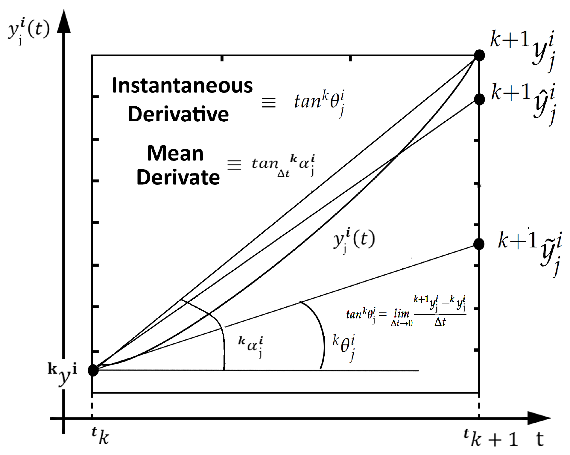
Figure 2.
A feed-forward neural network project with the concept of mean derivative functions.
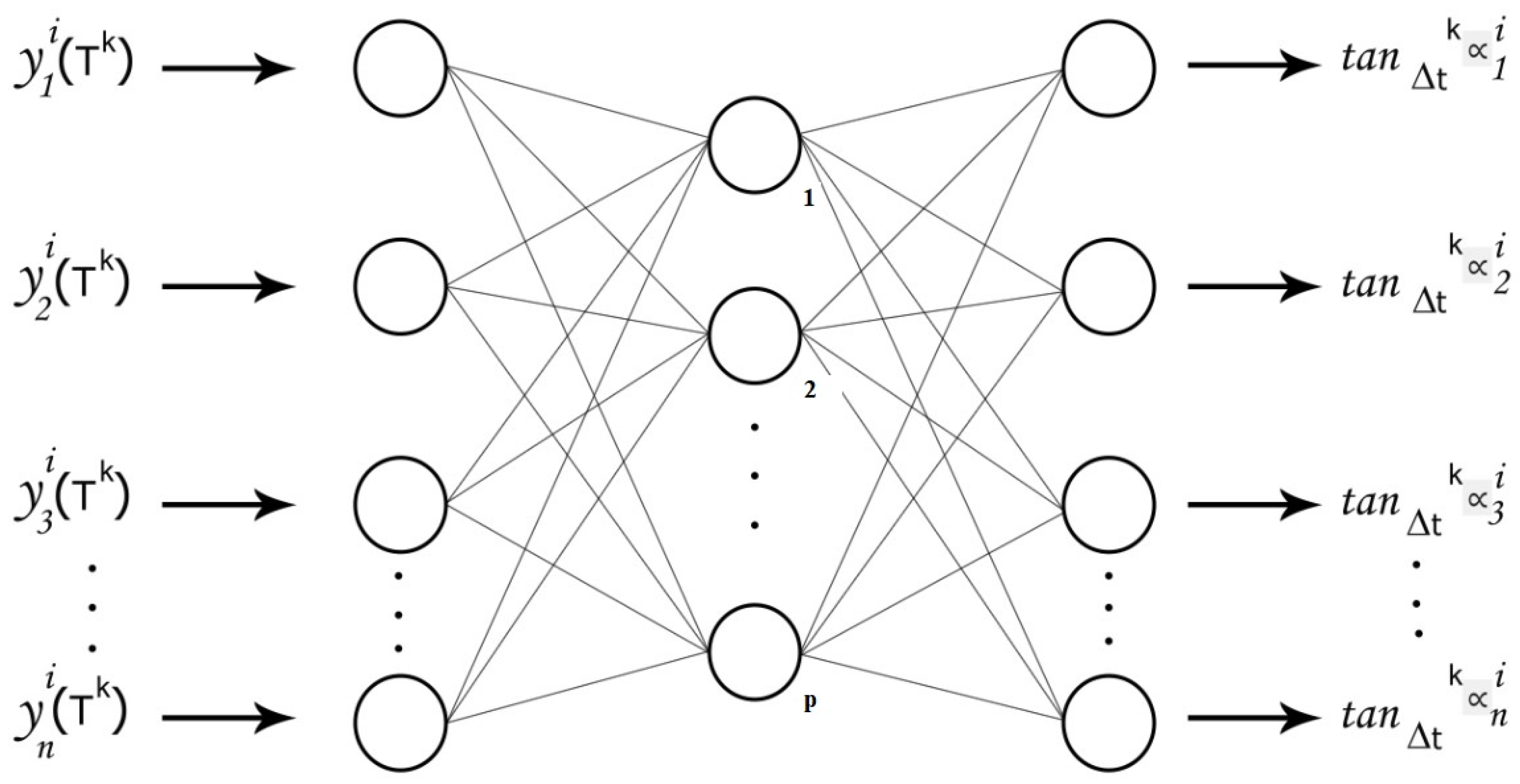
Figure 3.
Mapping scheme used to characterize the discretization of the solution obtained through E-TUNI (Source: see [19]).
Figure 3.
Mapping scheme used to characterize the discretization of the solution obtained through E-TUNI (Source: see [19]).
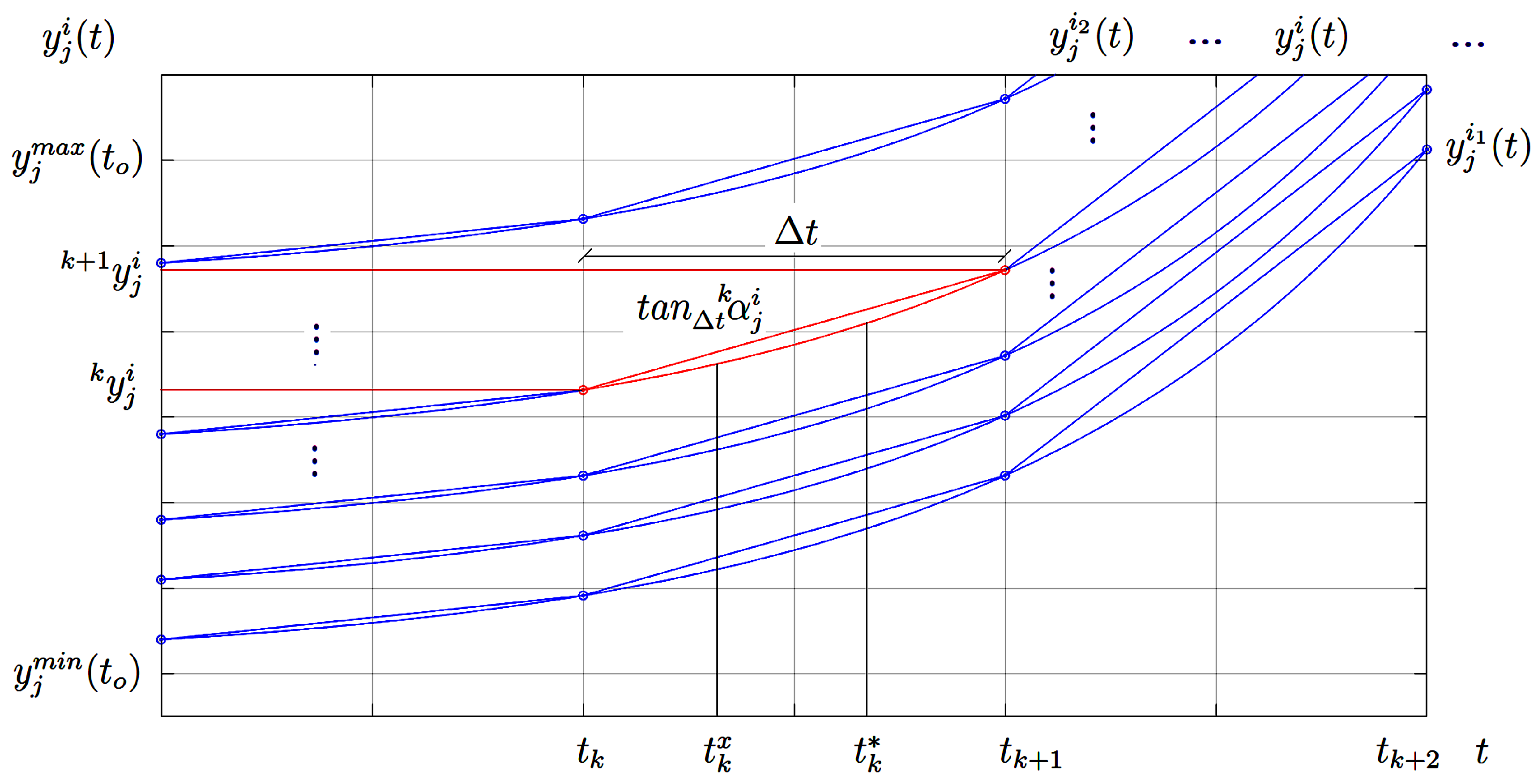
Figure 4.
Analytical solution of the dynamical system presented in example 1.
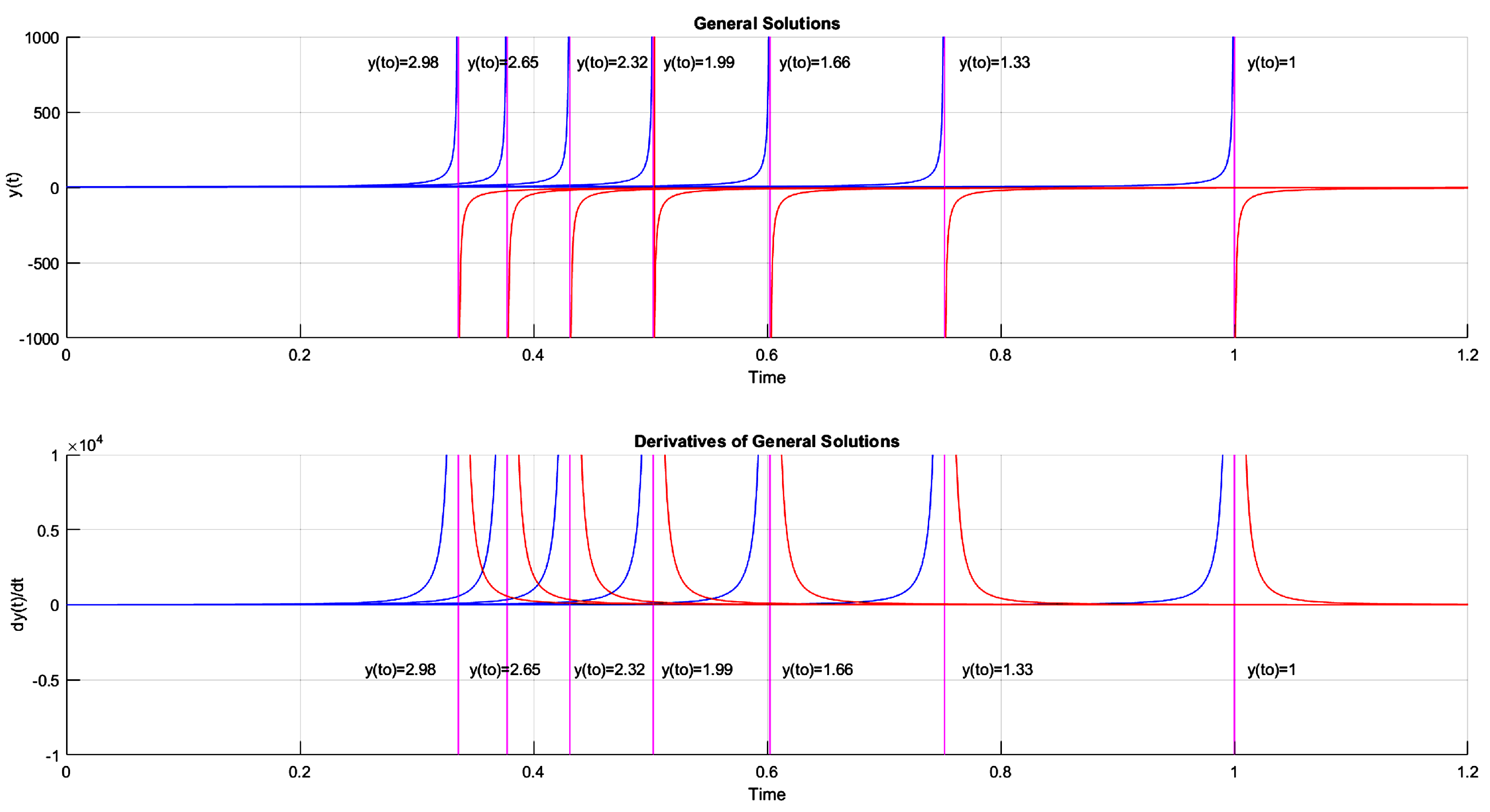
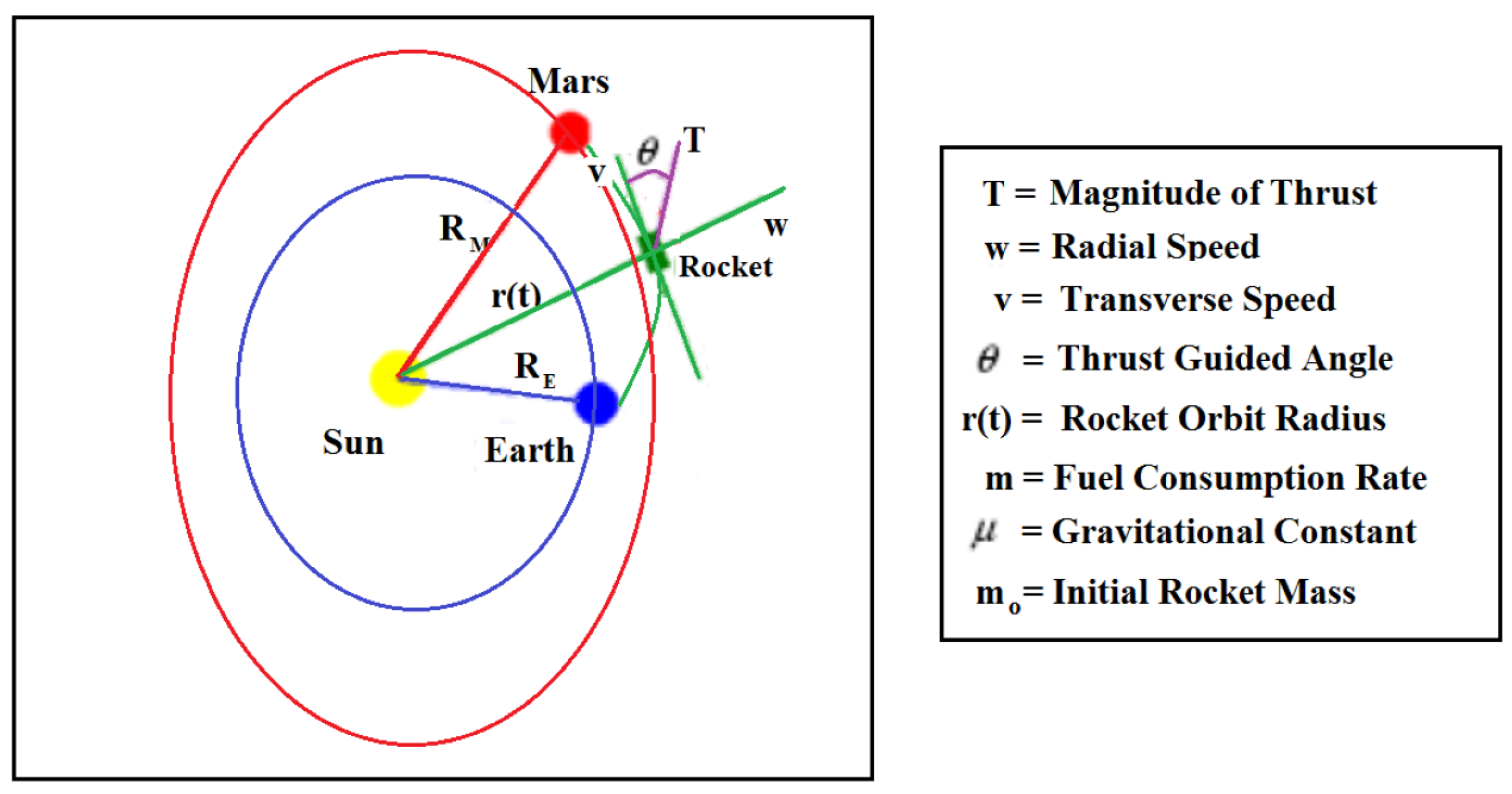
Figure 6.
Orbit radius trajectory for and .
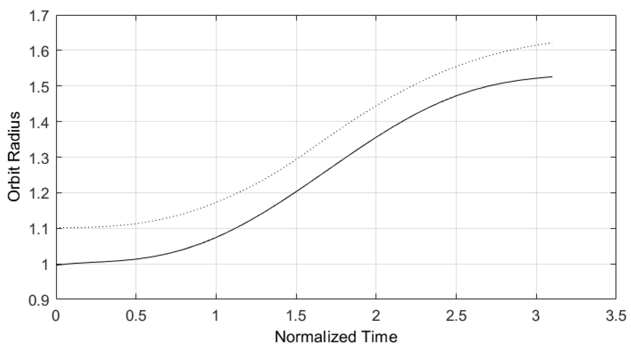
Figure 7.
Rocket angle thrust estimated by predictive control structure designed with E-TUNI and referring to Figure 6.
Figure 7.
Rocket angle thrust estimated by predictive control structure designed with E-TUNI and referring to Figure 6.
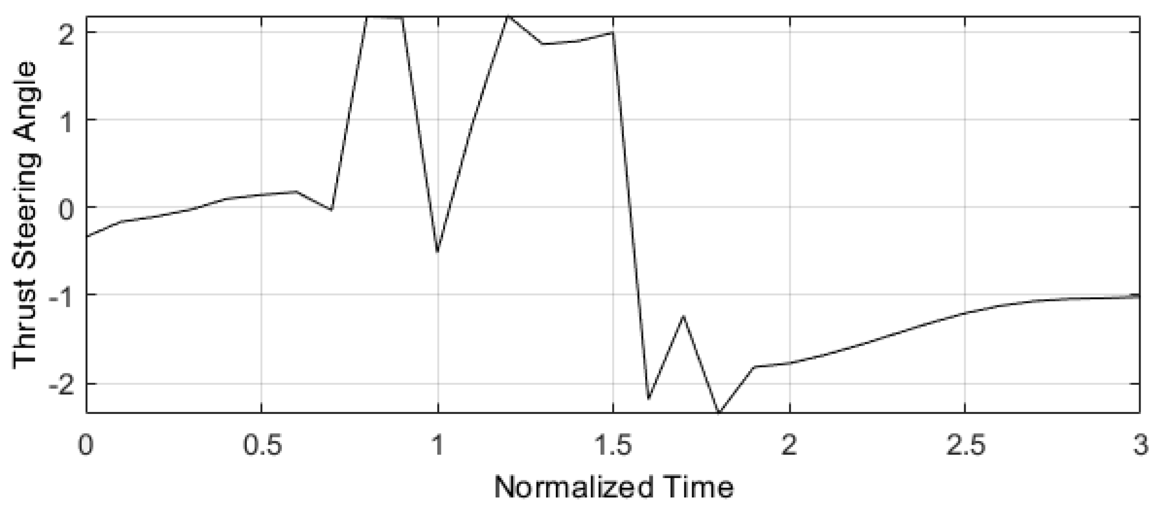
Figure 8.
Orbit radius trajectory for and .
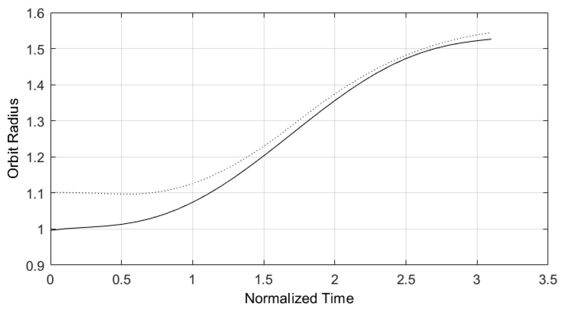
Figure 9.
Rocket angle thrust estimated by predictive control structure designed with E-TUNI and referring to Figure 8.
Figure 9.
Rocket angle thrust estimated by predictive control structure designed with E-TUNI and referring to Figure 8.
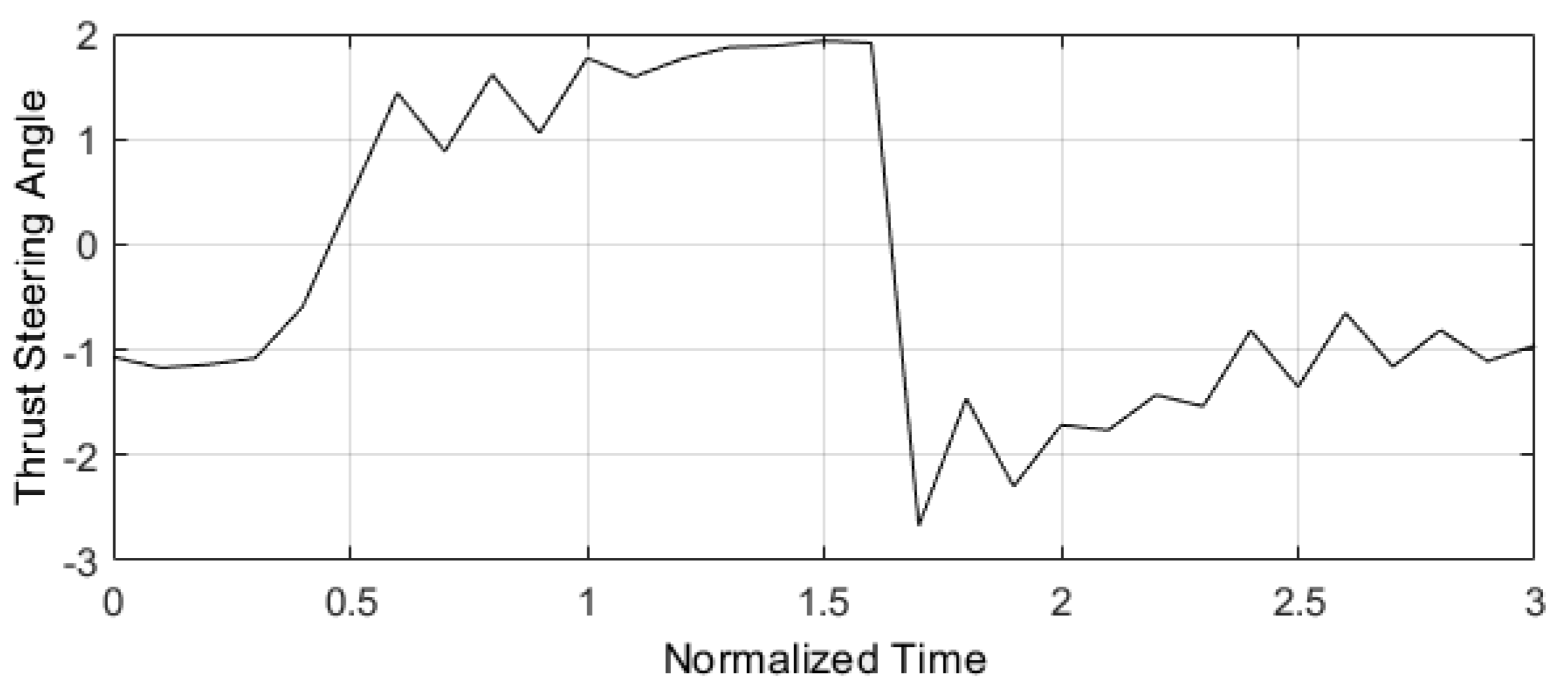
Figure 10.
Orbit radius trajectory for and (Source: see [16]).
Figure 10.
Orbit radius trajectory for and (Source: see [16]).
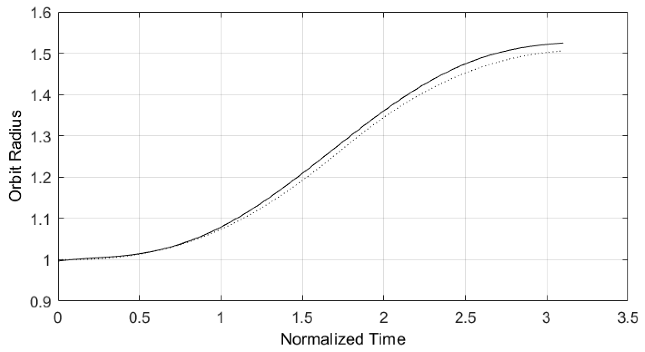
Figure 11.
Rocket angle thrust estimated by predictive control structure designed with E-TUNI and referring to Figure 10 (Source: see [16]).
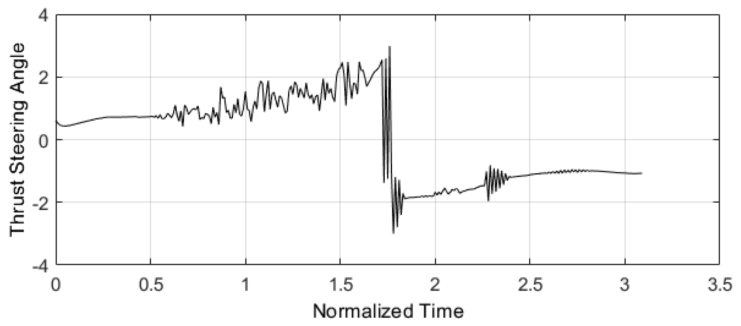
Figure 12.
The E-TUNI was designed with several distinct integration steps.
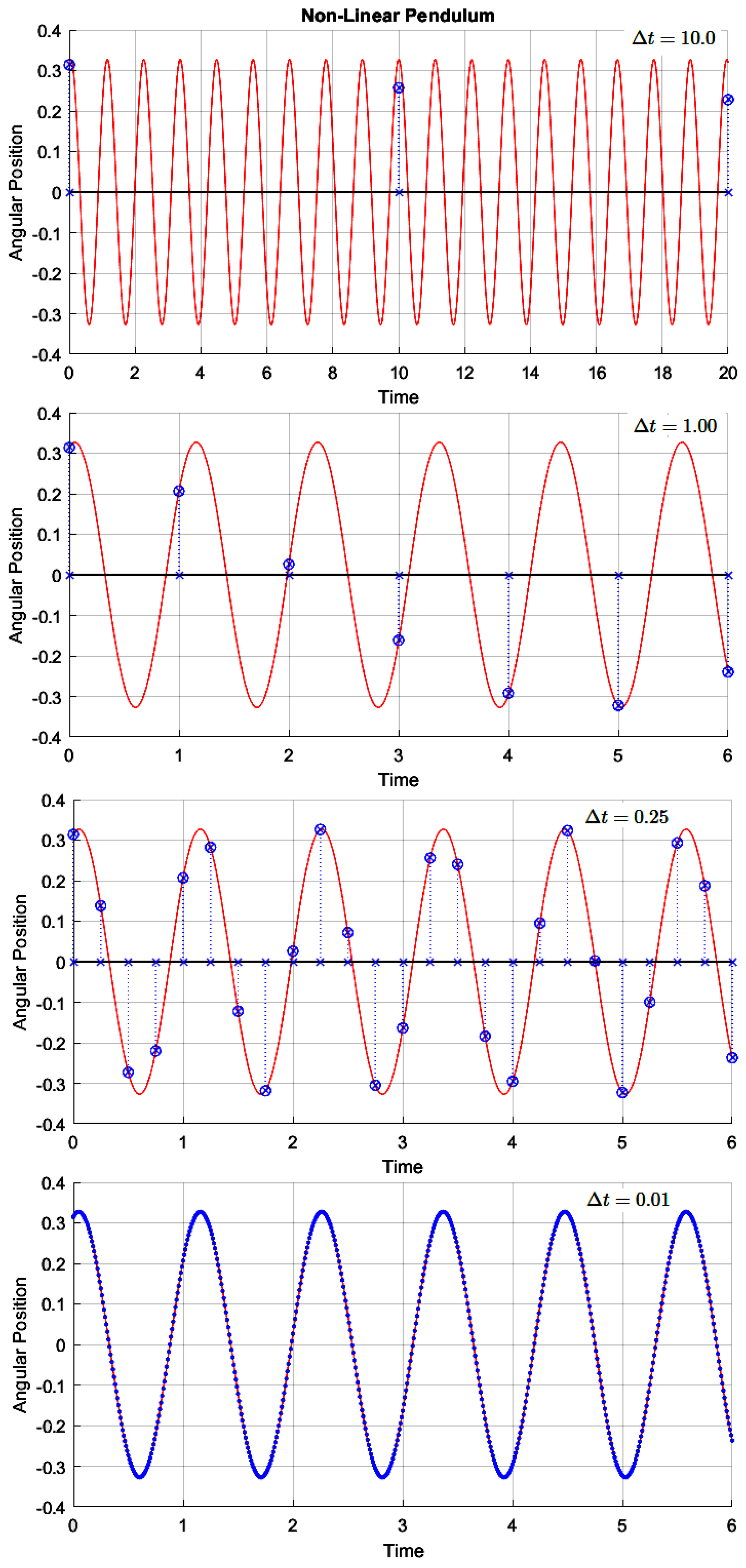
Figure 13.
The E-TUNI equivalent to the previous figure, but with the mean derivatives and interpolating parabolas present.
Figure 13.
The E-TUNI equivalent to the previous figure, but with the mean derivatives and interpolating parabolas present.
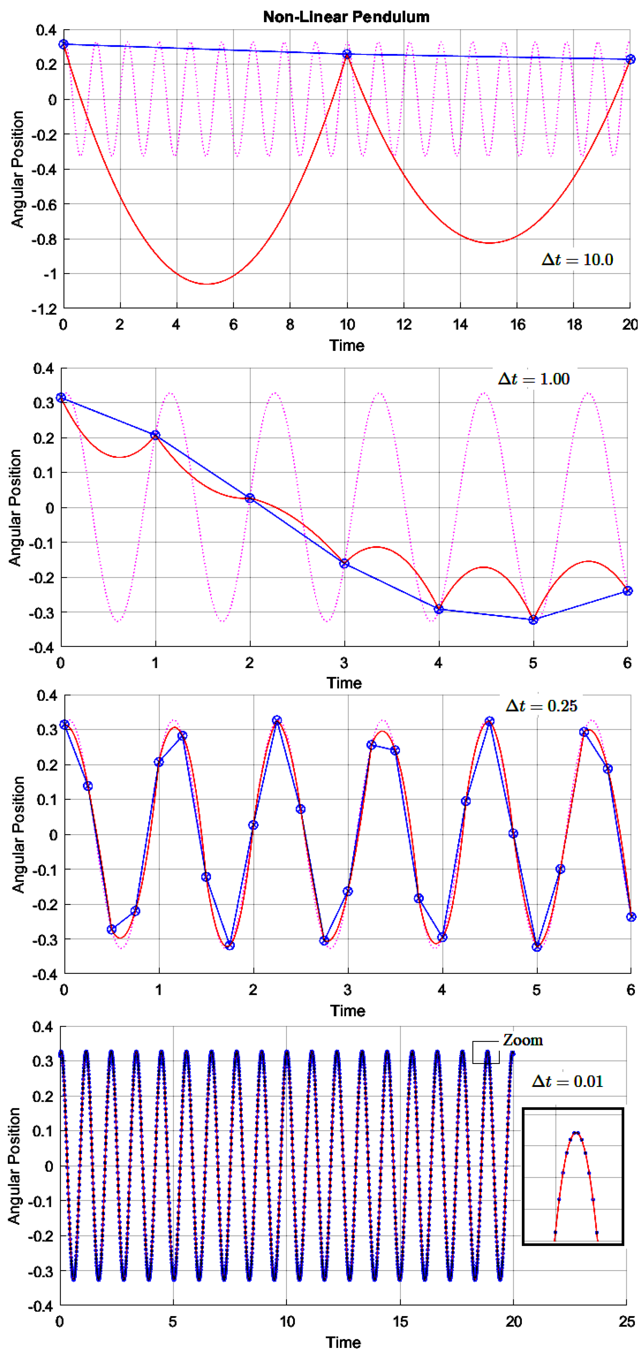

Table 1.
Coordinate points within the interval .
| n | Time | Determining Form | |
|---|---|---|---|
| 1 | Initial Instant | ||
| 2 | Given by E-TUNI | ||
| 3 | Output of net | ||
| 4 | From Equations (28) or (29) |
Table 2.
Summary of training performed for example 3.
| MSE of Validation Patterns | Direct Approach | |
|---|---|---|
| - | Instantaneous Derivatives | |
| Mean Derivatives | ||
| Mean Derivatives | ||
| Mean Derivatives | ||
| Mean Derivatives |
Disclaimer/Publisher’s Note: The statements, opinions and data contained in all publications are solely those of the individual author(s) and contributor(s) and not of MDPI and/or the editor(s). MDPI and/or the editor(s) disclaim responsibility for any injury to people or property resulting from any ideas, methods, instructions or products referred to in the content. |
© 2025 by the authors. Licensee MDPI, Basel, Switzerland. This article is an open access article distributed under the terms and conditions of the Creative Commons Attribution (CC BY) license (http://creativecommons.org/licenses/by/4.0/).
Copyright: This open access article is published under a Creative Commons CC BY 4.0 license, which permit the free download, distribution, and reuse, provided that the author and preprint are cited in any reuse.


