
Submitted:
05 December 2024
Posted:
06 December 2024
You are already at the latest version
Abstract
This paper extends Lyapunov stability theory to mixed fractional-order direct model reference adaptive control (FO-DMRAC), where the adaptive control parameter is of fractional order, and the control error model is of integer order. The proposed approach can also be applied to other types of model reference adaptive controllers (MRAC), provided the form of the control error dynamics and the fractional-order adaptive control law are similar. The paper demonstrates that the control error will converge to zero, even if the derivative of the classical Lyapunov function V is positive during a transient period, as long as V(e,ϕ) tends to zero as time approaches infinity. Finally, the paper provides application examples that illustrate both the convergence of the control error to zero and the behavior of V(e,ϕ).
Keywords:
Lyapunov function
; fractional order control
; fractional order direct model reference adaptive control (FO-DMRAC)
; convergence of the control error
1. Introduction
The principal aim of this paper is to show that the control error for some class of fractional order dynamic systems as the fractional order direct model reference adaptive control (FO-DMRAC) tend to zero as time tend to infinite using the classical Lyapunov stability approach.
The idea is not to show the performance of the controllers, but rather to show that although some of the conditions of the Lyapunov method () are not met for all , the control error converges to 0 as long as the limit of tends to zero as t tends to infinity, where is the plant output and is the reference model output.
It is important to mention that the classic Lyapunov method has been used, avoiding conceptual complexities as much as possible.
Many of the approaches applied to fractional adaptive systems use fractional (and not integer) derivatives of the Lyapunov function, achieving at most, demonstrate stability of the control error, but not convergence of this error to 0 [1,2,3].
Furthermore, many of these approaches are applied to fractional order systems with adaptive laws also of fractional order, facilitating the stability analysis for such systems. However, in most cases, the systems are of integer order and not fractional. Using the aforementioned approaches, it has only been possible to establish, that the limit of the integral of the mean square error to infinite grows at most with a certain speed (, ), which is useful but does not allow to establish convergence of the error itself to 0 [4,5].
Other approaches have used the gradient technique, but the error model dynamic is of fractional order [6,7].
Finally, to carry out this analysis, the adaptive error model 3 has been used in which there is no access to the system's states, making the analysis more complex.
The organization of the paper is as follows. Section 2 presents the classical or integer order implementation of the direct model reference adaptive control (IO-DMRAC). Section 3 shows some basic concepts and important results of the fractional calculus which will be the basis for analyzing the FO-DMRAC systems stability. Section 4 shows some of the difficulties in proving convergence of control error to 0 and the approach to establish such a convergence. In Section 5, simulation results are presented considering various examples that show the convergence to 0 of the control error and the behavior of the function. Finally, in Section 6 some conclusions are drawn.
2. Control Model System
Figure 2 shows a simplified block diagram for the classical or integer order Direct Model Reference Adaptive Control (DMRAC), in which control parameters and are adjusted using their corresponding adaptive laws to keep the control error as small as possible.
2.1. DMRAC Algorithm
The objective of the MRAC is to minimize the control error . In the DMRAC approach, for the adjustment of the controller parameters, it is not relevant that asymptotic convergence to the ideal parameters occurs, making the implementation simpler since the identification block is avoided [8].
Therefore, the DMRAC adaptive control scheme of a linear (or linearized) nth order plant, with relative degree 1 is shown in Figure 4, where only the control error is accessible (Error Model 3) but not the whole state error vector (Error Model 2), in which case, the analysis for determining stability conditions is simpler [8].
Figure 3 shows the block implementation of the classical DMRAC in more detail.
In which, the control law has the form
are the controller parameters and the auxiliary signals respectively, and , is the order of the plant.
are the parameters error vector controller
are the ideal controller parameters.
The auxiliary signals are defined by
with , and is any arbitrary stable and controllable pair, with a Hurwitz matrix.
For simplicity, we choose in the controllable canonical form. Furthermore, when , the control parameters for the classical or integer order adaptive laws (IO-DMRAC) can be chosen as:
On the other hand, for the fractional order adaptive laws (FO-DMRAC) case, these adaptive laws can be written as
3. Fractional Calculus Preliminaries
In this section we present some definitions and the main advances in the stability of fractional order model reference adaptive control systems.
3.1. Basic Concepts of Fractional Calculus
The basic definitions of fractional derivative and integral most used in engineering are presented [9,10] that will be useful for the implementation of the FO-DMRAC control.
Definition 1 [10]. The Riemann-Liouville fractional integral of order of a function is defined by
where is the Gamma function defined as
Some additional lemmas and a theorem are important for the stability analysis of fractional order adaptive control systems, which will be mentioned and whose proofs will be referenced in what follows.
3.2. Principal Adavances in Stability of Fractional Order Systems
Theorem 1. Let the state error and the control error be represented by equations
where is a Hurwitz matrix and such that given a matrix . Then, there exists a matrix such that
whose adaptive adjustment laws, to estimate the unknown controller parameters, are given by
where is the gain of the plant, which is unknow, but the sign is known. Also, and . Then, if and are differentiable and uniformly continuous functions, it holds that
- a)
- The parametric error , the state error and the control error remain bounded for all time.
- b)
- Furthermore, if the auxiliary signal is bounded, then and also remain bounded.
- c)
- The mean value of the squared norm of the state error is , or equivalentellywhere means that the speed of converges to zero is higher than . The proof of this theorem can be found in [3].
Remark 1. This theorem applies to system whose relative degree is grater than 1 as long as the model trasfer function is strictly positive real. Otherwise, it is necessary to modify so that it meets this condition.
From Theorem 1, since with a constant vector, then, the control error also will be .
if (c) holds, it must also hold for the mean value of the square norm of , since with a vector whose components are constants.
There is a lemma that relaxes the hypothesis (b) imposed from Theorem 1 when (i.e. the error model equation is of integer order), therefore all the internal signals are bounded and there is no need to impose the boundedness condition over . The proof of this lemma can be found in [13,14].
Furthermore, as the auxiliary signal is bounded and Theorem 1 guarantees (c), then the squared norm of the control error , also tends to 0 as t tends to infinity. That is
Therefore, the stability of the proposed FO-DMRAC is guaranteed.
Nevertheless, it is not possible to conclude convergence of the errors ( and ) to 0 as t tends to . Also, it is still a pending issue to prove the analytical differentiability of .
The high frequency gain of the plant is supposed to be unknown but its sign is assumed to be known (.
4. Some Issues That Difficult to Prove Convergence of Errors to 0 in Adaptive Fractional Order Systems
In the very well-known classical (or integer order) DMRAC, the proof of the convergence of the state error and the control error ( and respectively) to 0 rests on the Barbalat Lemma. That is, the derivative of the Lyapunov function
Then, using Barbalat Lemma we can conclude that the state error tends to 0 () and therefore, the control error also tend to 0 () [8].
Nevertheless, even that is not explicitly mentioned in the literature, because of the above, it must also be satisfied that .
In the case of mixed fractional order direct model reference adaptive control (FO-MRAC), there is not an equivalent Barbalat Lemma, therefore, it is not possible to conclude the convergence of the state error and the control error to 0.
If we write the Lyapunov function for the mixed adaptive system, we have (considering, from Figure 3, for simplicity)
therefore,
As we can see, it is not easy to know the sign of the second term or the term
with. To make easier the notation, we can make the variable change , therefore . Then, (11) could be re-written as
By Lemma 2 [11,12] we know that is boundness. By part (a) of Theorem 1, is boundness, therefore, (when tends to infinity) by Caputo derivative property. Moreover, as is boundness by the same theorem. Then, (12) is a boundedness term.
Still, we cannot prove that the term
Remark 2. If the signals are of the PE type (Persisting Excitation type) class of an adequate order, could converge to 0, but this is more related to the case of identification problems [8,13]. In the direct model reference adaptive control (DMRAC), not necessarily.
Even in this case, we can only show that but it is not enough to conclude that or and thus, also conclude that . Remember that Q is a constant and symmetric matrix.
Therefore, we need to explore what happens with the term inside the parenthesis. That is, the term .
First, we know that all the signal inside the parenthesis is boundedness, then
because as we show before, by Caputo derivative property, , as t tends to , because the term will be at least constant. Then, as is a bounded signal, if then and also and therefore and that will be the prove for the convergence to 0 of all errors (state error and control error ). But we are assumed that which is not possible to stablish a priori.
It is important to mention that several fractional adaptive systems present this behavior. That is, and . In the simulation results section (Section 5) we will show some examples that show this behavior for both, stable and unstable systems.
Now, from (7), as is arbitrary, as long as we can choose , therefore, (7) can be re-written as
, which give a term that is divide by . Even more, as part (a) of Theorem 1, is boundedness or by part (b) of the same theorem, is boundedness and as is part of (5), where all the other terms are boundedness, then must be boundedness, therefore the numerator of (5) can be infinite or constant (if is square integrable), then, we can use L’Hopital rule, that is
Then, since with a constant vector, then which mean that the control error tends to 0 conform t tends to . Therefore, we have proven the convergence of the state and control error to 0 which is new for fractional order direct model reference adaptive control systems (FO-DMRAC). Also, this result means that as in the integer order case.
5. Simulation Results
In this section we will show some examples (of different relative degree plants) that support what has been developed and conclude in section 4. The simulations were performed using Matlab-Simulink [14,15]. For all examples, zero initial conditions were considered.
For simplicity of the analysis but without loss of generality is considered. Then, as it was said before (9), a typical Lyapunov function can be choose such as . Therefore
. If , then, the above term can be rewritten as
Unlike the classic case, in (13), a term with a fractional derivative appears. For doing the simulation analysis, the designer can choose any such as . In this case, we will choose .
In the mixed FO-DMRAC control case where error model dynamics is of integer order and the adaptive laws are fractional (see Equation (1)), the dynamic of the state error , considering the plant together with the controller (error model 3) [13], is
where
and
Although from a theoretical point of view, it is not necessary to calculate the value of from since it is enough that the conditions of the Meyer-Kalman-Yakubovich (MKY) lemma are met, it is important for the purposes of carrying out the calculation of .
Next, we present some examples to show the behavior of the control error and the derivative of the Lyapunov function that confirm the convergence to 0 of which is the main result of this paper and it was proven in the previous section.
5.1. Scalar Stable Plant
Example 1: (and

Table 1.
FO-DMRAC implementation for a stable plant.
| Plant model | Reference Model |
|
. . . . |
. . . . . |
Remark 3. In the scalar case, and where and are the ideal control parameters and is the control law.
Then, using MKY lemma, that is, for any exist a such that
we may calculate , and for the system of Example 1 and thus, be able to calculate .
In this example, , , and .
The fractional adaptive laws were implemented using the Ninteger Toolbox [15]. Specifically, the NID block was used based on the Oustaloup method [16].
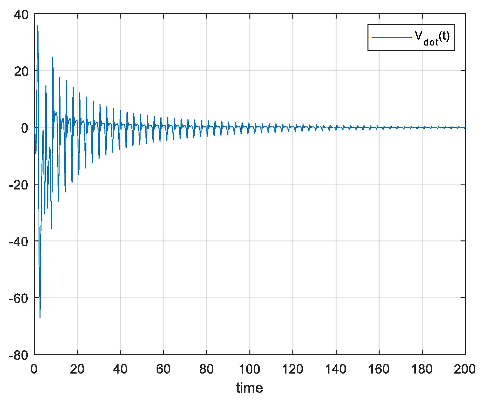
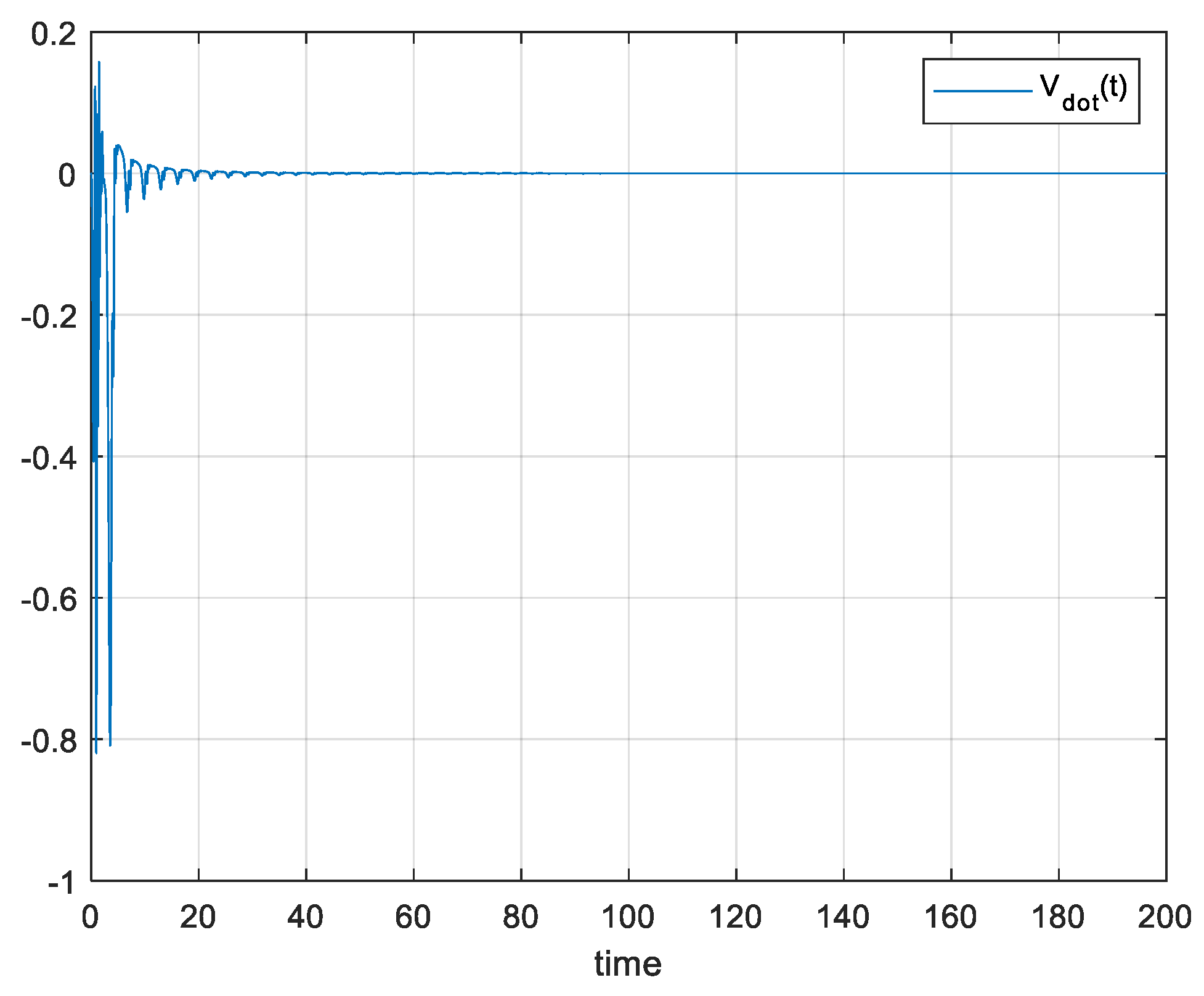
Figure 4 shows the plant response , reference output and control error respectively. From Figure 5 we can see the evolution of respectively.
Figure 4.
(a) FO-DMRAC reference output, response and (b) control error when .
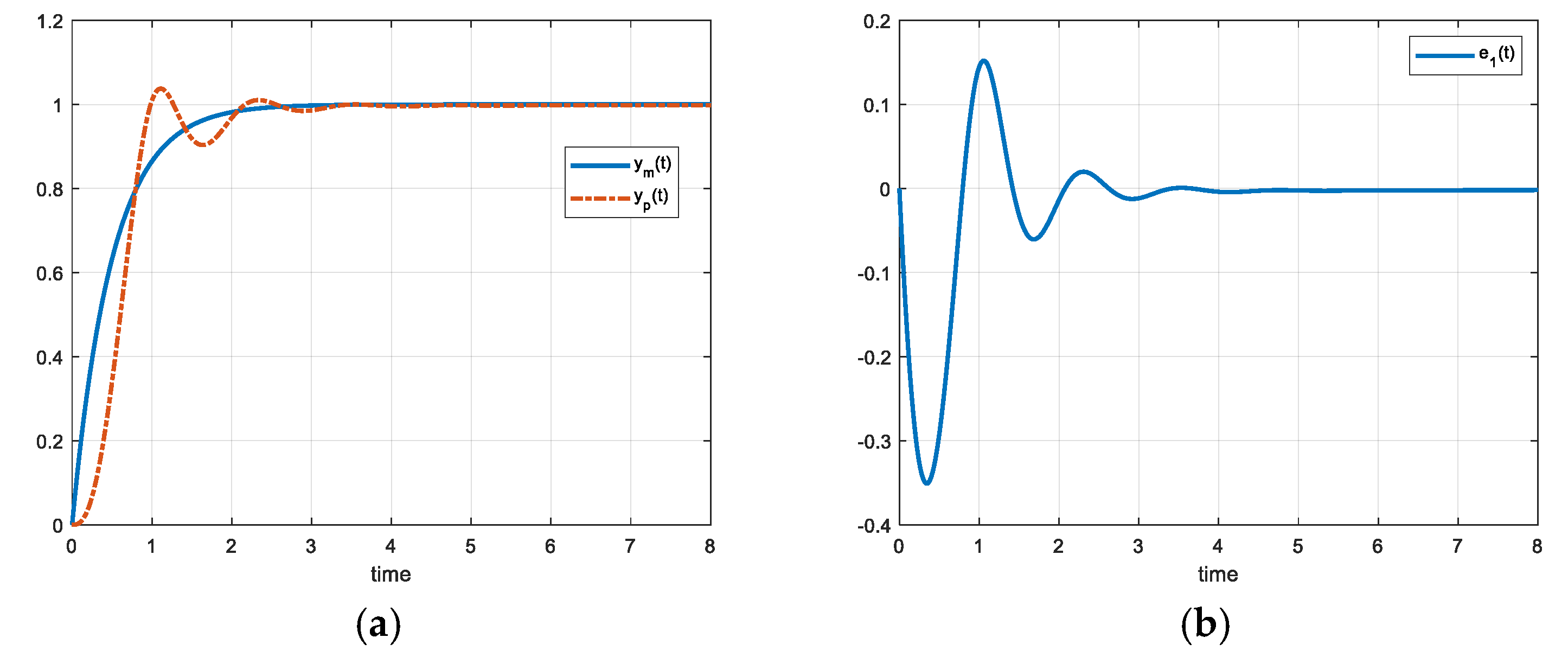
Also, from Figure 4 and Figure 5 it can be seen that the control error converges to 0 and can be greater than 0 in some time intervals, but also converge to 0 conform tends to such as the classical case.
5.2. Scalar unstable plant
Example 2: (and
Table 2.
FO-DMRAC implementation for an unstable plant.
| Plant model | Reference Model |
|
. . . . |
. . . . . |
The next figures show similar convergence behavior as the graphics of Example 1 for the unstable plant.
Figure 8.
(a) FO-DMRAC reference output, response and (b) control error when .
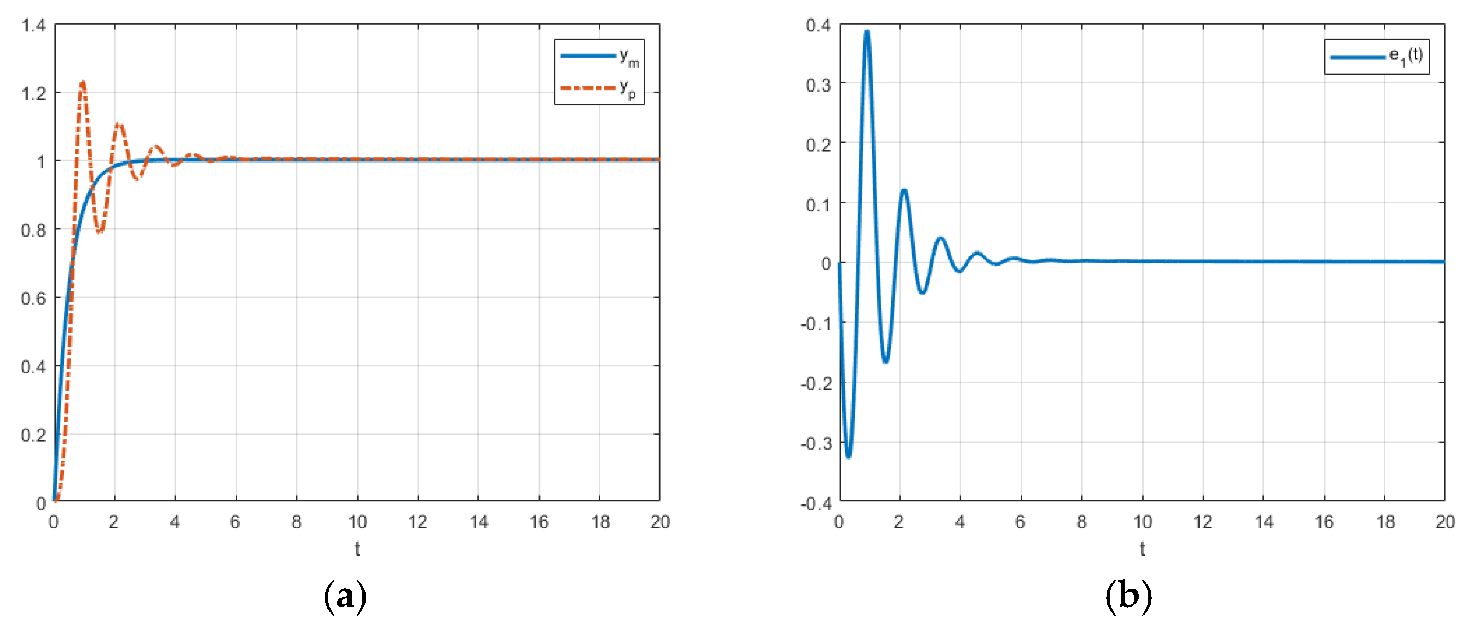
Figure 9.
FO-DMRAC graph of when .

5.3. Vectorial Case (stable Plant)
Example 3: (and
Table 3.
FO-DMRAC implementation.
| Plant model | Reference Model |
|
. . |
. . . . Controllable canonical form: |
|
, | |
Remark 4. The reference model transfer function has been changed (order 2) just to match the conditions for finding the control ideal parameters , but the behavior is the same as the original transfer function .
Control Laws:
Note: and
Internal auxiliary signals:
Fractional order adaptive laws:
Remark 5. is a diagonal matrix where . For practical implementation simplicity, we choose (identity matrix of appropriated dimension).
are the parameters error vector controller and are the ideal controller parameters.
Finally, , whose eigenvalues are -1, -2, -1 and -1 therefore is Hurwitz. Also, if which is a symmetrical and positive defined matrix, then which is also a symmetrical and positive defined matrix that satisfies the MKY Lemma. That is
Figure 12.
(a) FO-DMRAC reference output, response and (b) control error when .
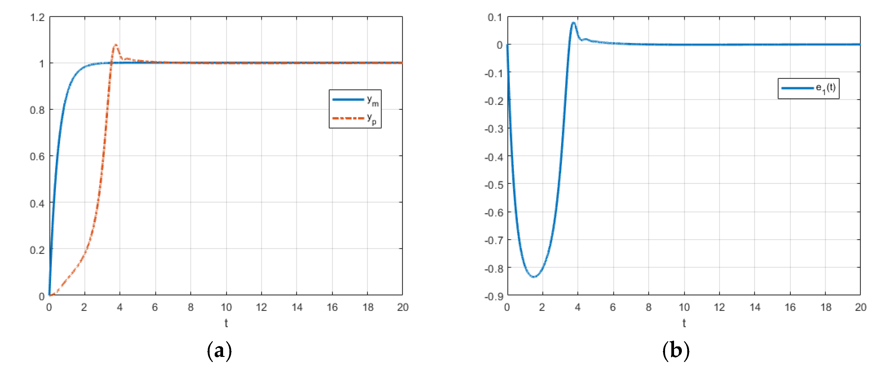
Figure 13.
FO-DMRAC graph of when .
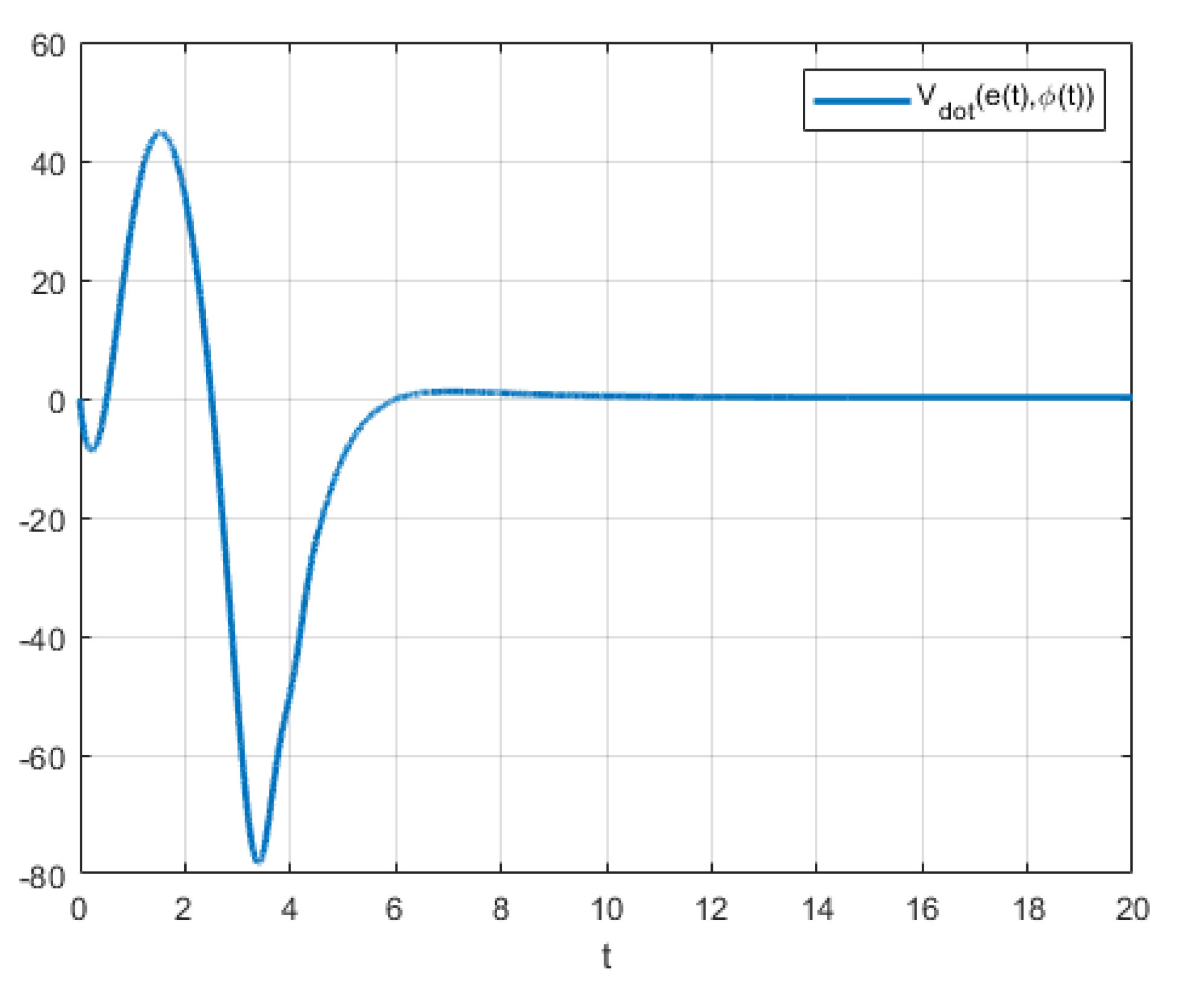
From Figure 12 it can see a similar behavior as the examples 1 and 2, that is, the plant output converges to the model reference output which is equivalent to saying that the control error tends to 0 as t tends to . Also, from Figure 13 we confirm that even if in some time intervals (mainly in the transient period), can be positive.
Now, changing the reference signal to a sinusoidal one as in the previous example, that is, , we obtain the following dynamic behavior which are show in the next figures.
Figure 12.
(a) FO-DMRAC reference output, response and (b) control error when .
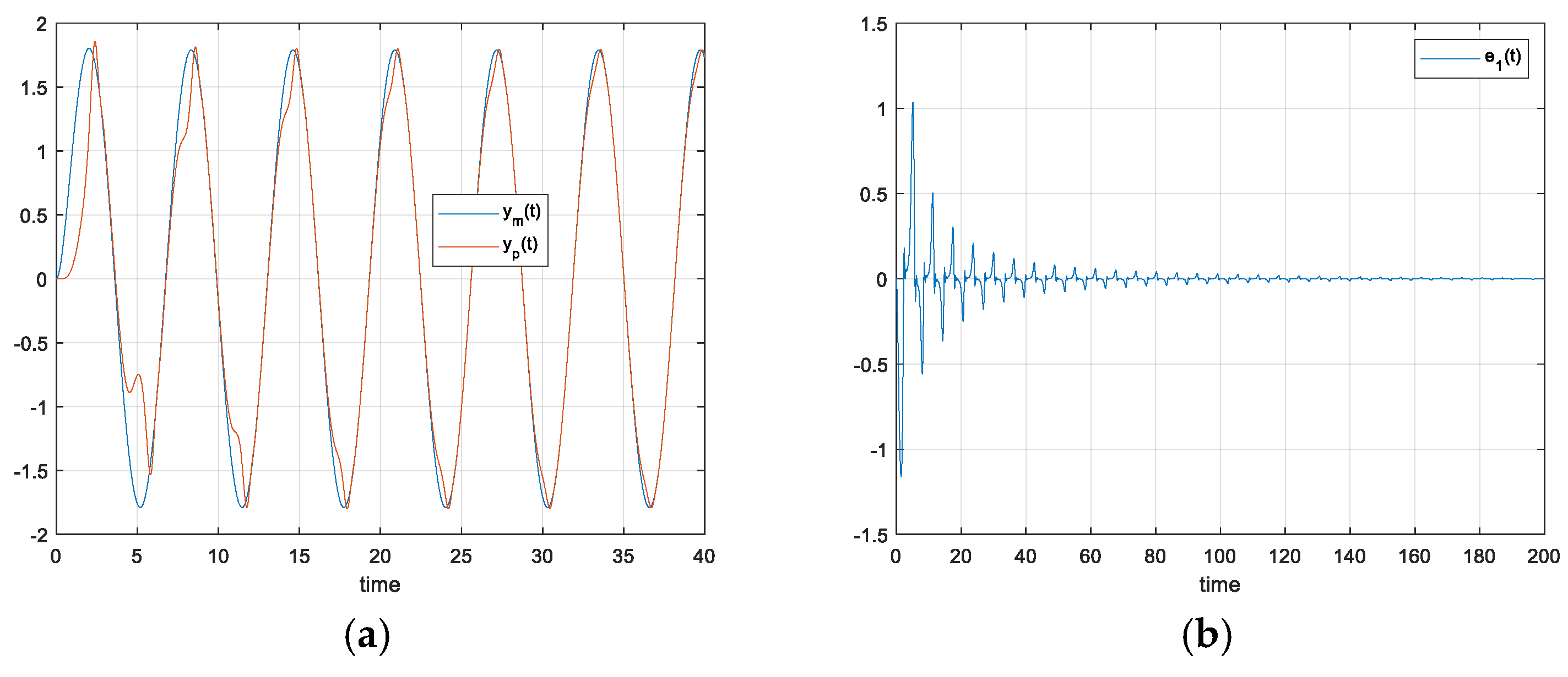
Figure 13.
FO-DMRAC graph of when .
Remark 5. These simulations are made to show that (control error converge to 0) in the case of fractional order model reference adaptive control implementation (FO-DMRAC) and not to show the performance of the controllers. Better performance can be achieved by using an optimization algorithm such as PSO [17] or another one, in such a way as to choose the fractional parameters and adaptive gains more conveniently.
Finally, it can be established new conditions of the Lyapunov method applied to FO-DMRAC. That is, let be a a continuous and derivable function, then
- i)
- ii)
- iii)
- If , then, , which implies that the control error also converge to 0.
6. Conclusions
In this article, we have proven that in the FO-DMRAC case, the control error converges to 0 even if the derivative of the Lyapunov function is greater than 0 in some time intervals (mainly in the transient periods). Some examples have been presented to show the convergence of the control error and the behavior of the function as approaches infinity.
One of the main difficulties in carrying out the synthesis of for simulation purposes is that we need to compute the ideal control parameters analytically and the matrix Q explicitly, which is not an easy task when the order of the plant to control grows in order. One practical approach to determine the ideal controller parameters is to implement the controller system using a Persistent Excitation (PE) reference input signal and wait for convergence. Sometimes, it could take a long time depending on the systems order because the higher the order, the more parameters we must compute.
In conclusion, the convergence of the state error and the control error to zero has been demonstrated for a class of fractional adaptive control systems (FO-DMRAC) using the classical Lyapunov approach avoiding additional complexities in the analysis. Previously, it had only been established that the mean square errors converge to zero as time approaches infinity; however, the convergence of errors themselves had not been explicitly demonstrated until now.
Author Contributions
Conceptualization and methodology, G.E.C.B.; investigation, G.E.C.B. and M.A.D.-M.; validation, G.E.C.B. and M.A.D.-M.; writing—original draft, G.E.C.B.; writing—review and editing, G.E.C.B., M.A.D.-M and L.B.M. All authors have read and agreed to the published version of the manuscript.
Funding
The authors are grateful for the support obtained from the Universidad Central de Chile. The data are contained within the article.
Acknowledgments
The research presented in this paper has been supported by the Faculty of Engineering and Architecture (FINARQ) of the Universidad Central de Chile.
Conflicts of Interest
The authors declare no conflicts of interest.
References
- M.A. Duarte-Mermoud, N. Aguila-Camacho, J.A. Gallegos, R. Castro-Linares, “Using General Quadratic Lyapunov Functions to Prove Lyapunov Uniform Stability for Fractional Order Systems”. Communications in Nonlinear Science and Numerical Simulation, Vol. 22, No. 1-3, May 2015, pp. 650-659, 2015.
- N. Aguila-Camacho, M.A. Duarte-Mermoud, “Boundedness of the solutions for certain classes of fractional differential equations with application to adaptive systems. ISA Trans. 60 (2016), 82-88;. [CrossRef]
- N. Aguila-Camacho, J. Gallegos, M.A. Duarte-Mermoud, “Analysis of fractional order error models in adaptive systems: Mixed order cases”, Fractional Calculus and Applied Analysis. Vol. 22, No. 4, 2019, pp 1113-1132, 2019.
- N. Aguila-Camacho, M.A. Duarte-Mermoud, J.A. Gallegos, “Lyapunov Functions for Fractional Order Systems”. Communications in Nonlinear Science and Numerical Simulation, Vol. 19, No. 9, 2014, pp. 2951-2957, 2014.
- Aguila-Camacho, N.; Duarte-Mermoud, M.A. “Boundedness of the solutions for certain classes of fractional differential equations with application to adaptive systems”. ISA Trans. 2016, 60, 82–88.
- Gallegos, J.A.; Duarte-Mermoud, M.A. Convergence of fractional adaptive systems using gradient approach. ISA Trans. 2017, 69, 31–42.
- Javier A. Gallegos; Manuel A. Duarte-Mermoud,“Impoved performance of identification and adaptive control schemes using fractional operators”, Int. J Robust Nonlinear Control.2021;31;4118-4130.
- K. S. Narendra and A. M. Annaswamy, Stable Adaptive Systems. Dover Publications Inc., 2005.
- A. Kilbas, H. Srivastava, and J. Trujillo, Theory and applications of fractional differential equations. Elsevier, 2006.
- K. Diethelem, “The Analysis of Fractional Differential Equations” Springer-Verlag, Berlin-Heidelberg, 2010.
- Gustavo E. Ceballos Benavides, Manuel A. Duarte-Mermoud, Marcos E. Orchard and Juan Carlos Travieso-Torres, “Pitch Angle Control of an Airplane Using Fractional Order Direct Model Reference Adaptive Controllers”, Fractal Fract. 2023,7, 342. [CrossRef]
- Gustavo E. Ceballos Benavides, Manuel A. Duarte-Mermoud, Marcos E. Orchard and Alfonso Ehijo, “Enhancing the Pitch-Rate Control Performance of an F-16 Aircraft Using Fractional-Order Direct-MRAC Adaptive Control”, Fractal Fract. 2024, 8, 338. [CrossRef]
- Narendra, K.S.; Annaswamy, A.M. Persistent excitation in adaptive systems. Int. J. Control 1987, 45, 127–160.
- The Math Works Inc. Control system toolbox user's guide. 1998. "http:\\www.mathworks.com".
- Valerio, D. & da Costa, “Ninteger: a non-integer control toolbox for matlab”. In Fractional Derivatives and Applications. OIFAC, Bordeaux, France, 2004.
- Sabatier, J.; Aoun, M.; Oustaloup, A.; Gregoire, G.; Ragot, F.; Roy, P. Fractional system identification for lead acid battery state of charge estimation. Signal Process. 2006, 86, 2645–2657.
- Maurice Clerc, “Particle Swarm Optimization”, ISTE Ltd, 2006.
Figure 2.
Classical DMRAC Block diagram.
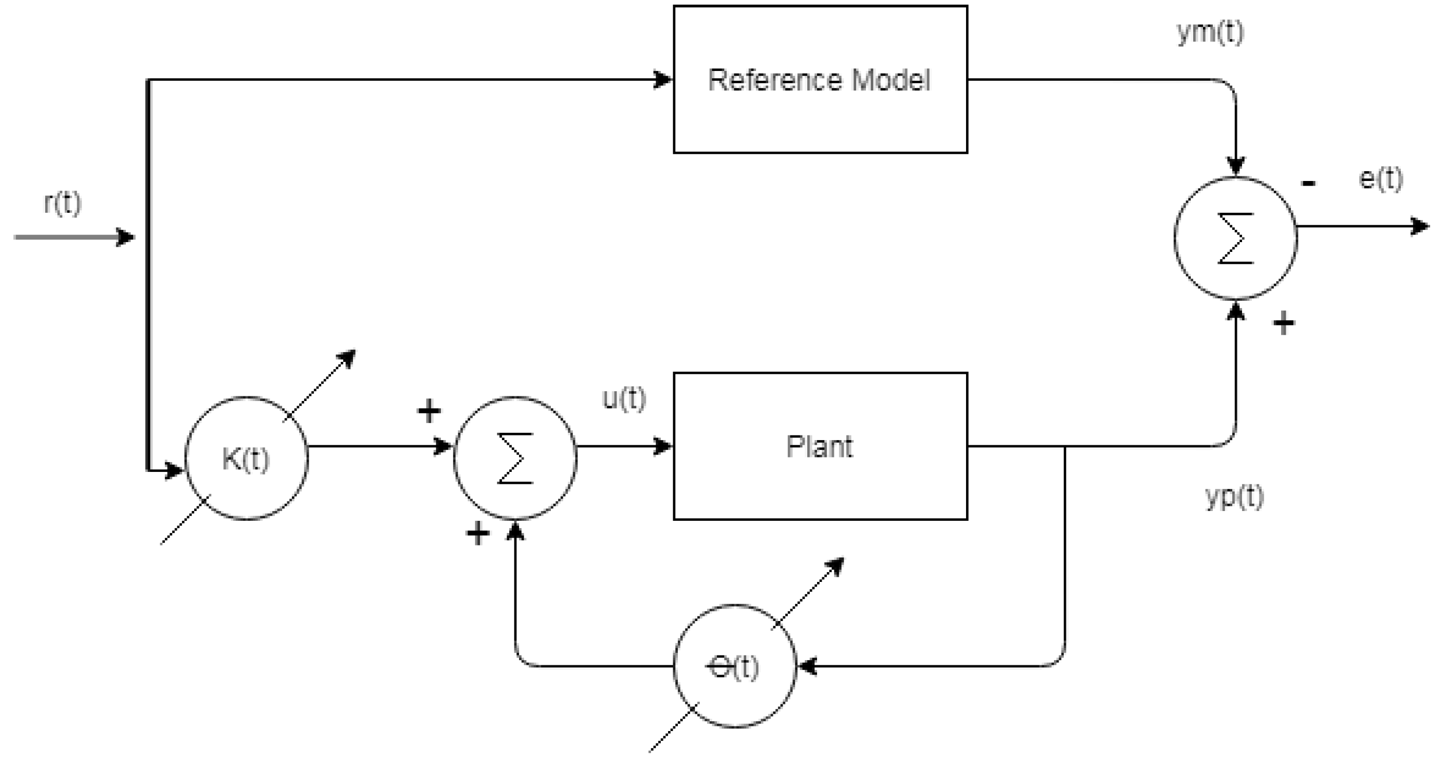
Figure 3.
DMRAC block diagram for Plant relative degree is 1 ().
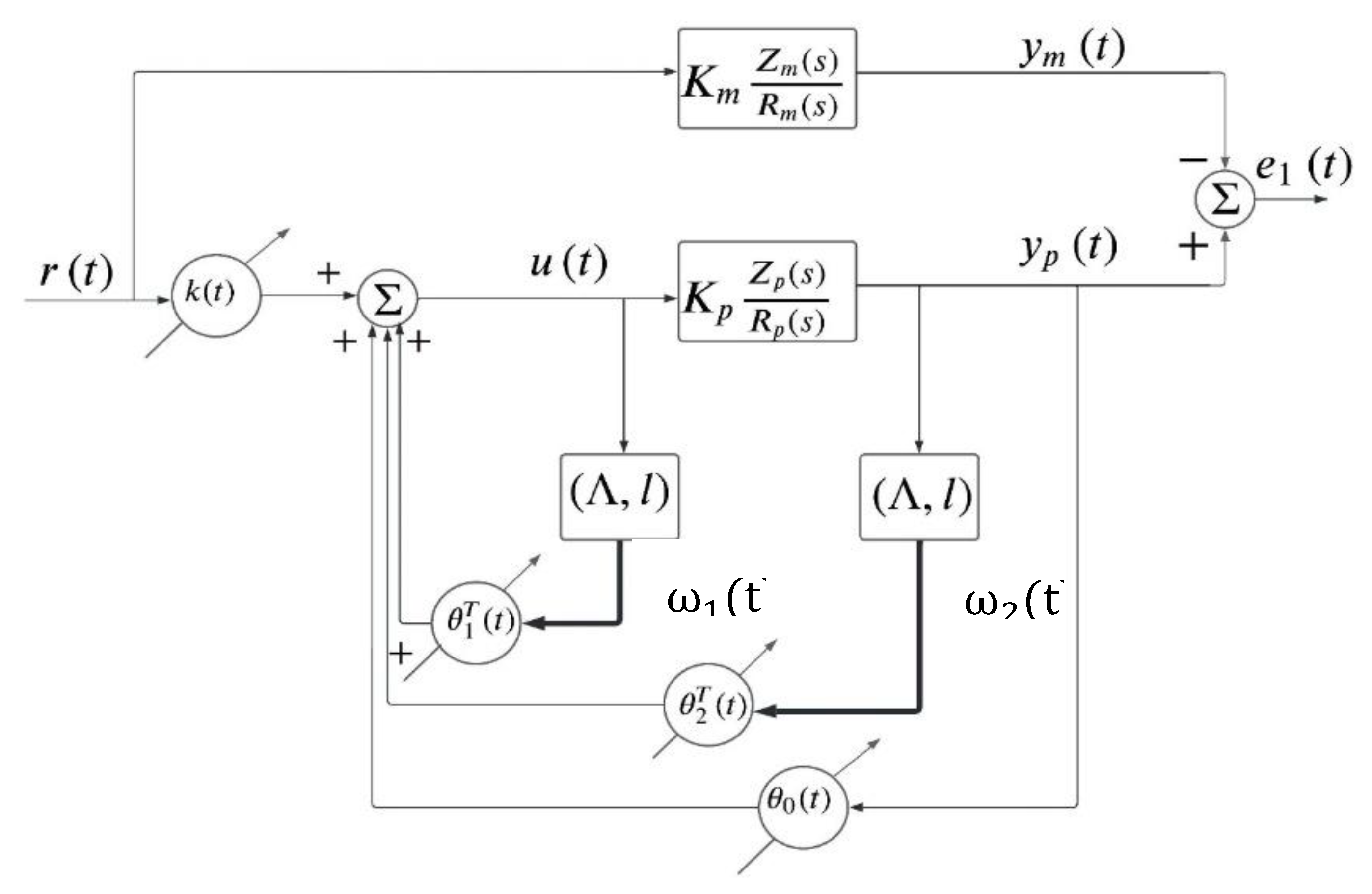
Figure 5.
FO-DMRAC graph of when .
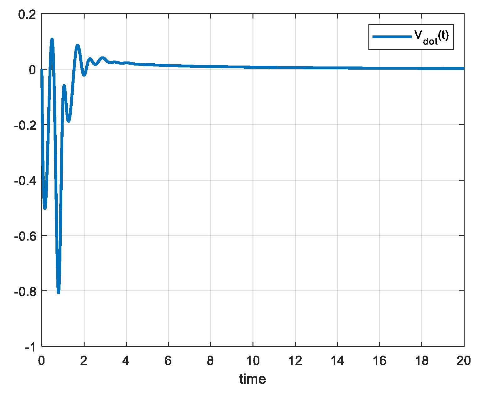
Figure 6.
(a) FO-DMRAC reference output, response and (b) control error when .
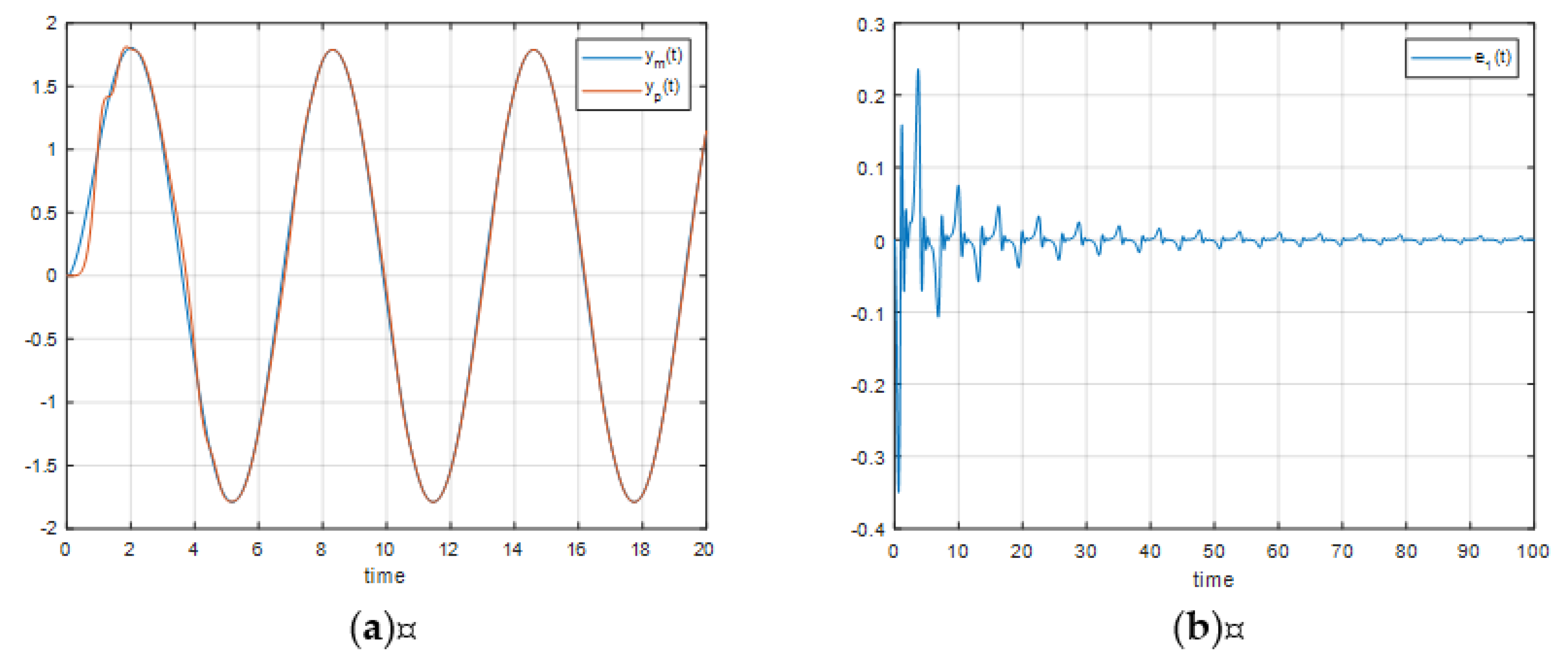
Figure 7.
FO-DMRAC graph of when .
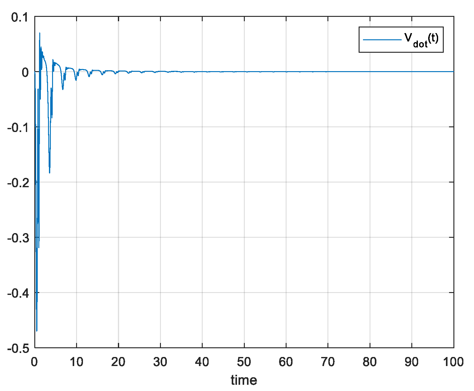
Figure 10.
(a) FO-DMRAC reference output, response and (b) control error when .
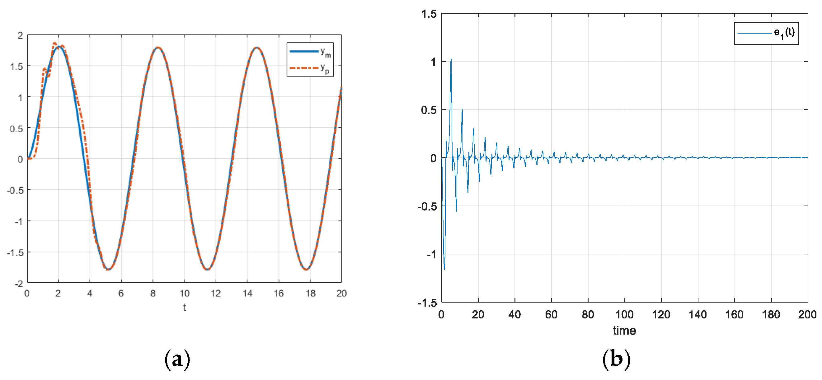
Figure 11.
FO-DMRAC graph of when .
Disclaimer/Publisher’s Note: The statements, opinions and data contained in all publications are solely those of the individual author(s) and contributor(s) and not of MDPI and/or the editor(s). MDPI and/or the editor(s) disclaim responsibility for any injury to people or property resulting from any ideas, methods, instructions or products referred to in the content. |
© 2024 by the authors. Licensee MDPI, Basel, Switzerland. This article is an open access article distributed under the terms and conditions of the Creative Commons Attribution (CC BY) license (http://creativecommons.org/licenses/by/4.0/).
Copyright: This open access article is published under a Creative Commons CC BY 4.0 license, which permit the free download, distribution, and reuse, provided that the author and preprint are cited in any reuse.


