
Submitted:
12 October 2025
Posted:
14 October 2025
You are already at the latest version
Abstract
This paper investigates the stability analysis and stabilization problems for a class of nonlinear time-delay systems described by conformable derivatives. We consider systems with one-sided Lipschitz nonlinearities and quadratic inner-boundedness conditions, which encompass a broad range of practical applications. Through the construction of appropriate Lyapunov-Krasovskii functionals, we develop novel linear matrix inequality (LMI) conditions for exponential stability of autonomous systems and practical exponential stability for systems subject to bounded perturbations. Furthermore, we propose state-feedback stabilization strategies that transform the controller design problem into a convex optimization framework solvable via efficient LMI techniques. The theoretical developments are comprehensively validated through numerical examples that demonstrate the effectiveness of the proposed stability and stabilization criteria. The results establish a rigorous framework for analyzing and controlling conformable fractional-order systems with time delays, bridging theoretical advances with practical implementation considerations.
Keywords:
conformable derivatives
; nonlinear time-delay systems
; exponential stability
; practical stability
; Lyapunov-Krasovskii functionals
; linear matrix inequalities
; state-feedback stabilization
; one-sided Lipschitz nonlinearities
; quadratic inner-boundedness
1. Introduction
Fractional calculus has become an essential mathematical framework for modeling complex physical phenomena with memory effects and hereditary properties [1,2]. Unlike classical integer-order calculus, fractional derivatives incorporate non-local operators that capture history-dependent behavior, making them particularly suitable for viscoelastic materials, biological systems, and anomalous diffusion. Among various fractional derivative definitions, the conformable fractional derivative introduced by Khalil et al. [1] and refined by Abdeljawad [2] has gained significant attention due to its mathematical simplicity and preservation of classical derivative properties. Subsequent generalizations by Zhao and Luo [3], Atangana et al. [4], Martínez et al. [5], and Sadek and Akgul [6] have further expanded the theoretical foundation, revealing additional properties and applications across scientific domains.
The adoption of conformable derivatives in this study is motivated by several compelling advantages over traditional fractional derivatives. Unlike Riemann-Liouville or Caputo derivatives, conformable derivatives preserve fundamental properties of classical calculus including the product rule, quotient rule, and chain rule, enabling more straightforward Lyapunov-based analysis and controller design. This mathematical elegance significantly simplifies stability analysis while maintaining the ability to capture memory effects and hereditary properties essential for modeling real-world systems. Furthermore, conformable derivatives offer computational advantages in numerical implementations and provide a more intuitive interpretation of fractional-order dynamics, making them particularly suitable for control applications where both theoretical rigor and practical implementation are paramount.
Parallel to these developments, time-delay systems have constituted a fundamental research area in control theory, owing to their prevalence in engineering applications ranging from chemical processes to networked control systems [7,8]. The presence of time delays can significantly impact system behavior, often leading to performance degradation, instability, or complex dynamical phenomena [9,10]. The intersection of fractional calculus and time-delay systems represents a natural progression for modeling systems exhibiting both memory effects and delayed interactions, with applications spanning nonlinear electrical networks [11], heat conduction [12], financial systems [9], and quantum control [13].
Within this context, conformable fractional derivatives offer particular advantages. Foundational stability results were established by Naifar et al. [14], while Luo et al. [15] investigated fractional exponential stability in conformable delayed systems with impulsive effects. Practical stability considerations have been addressed by Aldandani et al. [16] and Kharrat et al. [17], who developed frameworks for systems with external disturbances. A significant challenge involves characterizing nonlinearities tractably yet accurately. The one-sided Lipschitz condition with quadratic inner-boundedness provides a powerful framework for describing broad nonlinearity classes with less conservative bounds than conventional Lipschitz conditions [18,19], enabling more accurate stability analysis and controller design.
Recent stabilization advances include guaranteed cost control with event-triggered mechanisms [22], observer designs for nonlinear tempered fractional-order systems [23], stabilization criteria for fuzzy delayed systems [24], and predictor-feedback methods with quantization effects [25]. Practical observer design techniques using Caputo fractional derivatives have been proposed by Naifar et al. [26]. Linear Matrix Inequalities (LMIs) have emerged as powerful tools, with applications spanning neutral systems with multiple delays [27], stabilization of feedforward nonlinear systems [28], and robust stability analysis of mechanical systems [29]. Beyond control, conformable derivatives have found utility in optimization contexts [30,31], soliton solutions [32], grey system modeling [33], and quantum control [13].
Recent stability methodologies continue to evolve, with Chen et al. [34] investigating delayed impulses, Zhang et al. [35] examining stochastic nonlinear delay equations, and event-triggered adaptive stabilization approaches [36]. Reduced-conservatism LMI conditions have been proposed for exact Takagi-Sugeno models [37], while specialized approaches address neutral-type bilinear systems [38], p-normal nonlinear systems [39], and systems with highly nonlinear impulses [40].
Despite these advances, significant research gaps remain in stability analysis and stabilization of conformable fractional-order systems with time delays. Many approaches exhibit conservatism in handling one-sided Lipschitz nonlinearities, lack comprehensive practical stability treatment under bounded perturbations, or provide limited constructive controller design methods. The integration of conformable derivative properties with sophisticated Lyapunov-Krasovskii functional constructions remains underexplored, particularly for LMI-based conditions that are computationally tractable and mathematically rigorous.
This paper addresses these challenges through the following key contributions:
- Novel LMI conditions for exponential stability of autonomous conformable time-delay systems with one-sided Lipschitz nonlinearities and quadratic inner-boundedness constraints
- Practical exponential stability criteria for perturbed systems with bounded disturbances, providing computable ultimate bounds
- State-feedback stabilization strategies for nominal and perturbed systems via convex optimization
- Systematic Lyapunov-Krasovskii functional construction tailored to conformable derivative properties
- Comprehensive numerical validation demonstrating effectiveness and applicability
2. Preliminaries
In this work, the subsequent notation is adopted: is the n-dimensional Euclidean space; contains all real matrices; I is the identity matrix; signifies the Euclidean norm for vectors; and are the smallest and largest eigenvalues of the matrix , in that order; is defined as ; and stands for the block diagonal matrix .
Definition 1
(Conformable Fractional Derivative). For a function f defined on the interval and a fractional order , the conformable fractional derivative starting from point p is given by the limit expression:
This definition extends to the left endpoint by continuity: if the right-hand limit exists, then we define .
Remark 1.
The definition presented above generalizes the concept introduced by Khalil et al., which corresponds to the specific case where the starting point p is zero. For notational convenience, we will use the shorthand in the subsequent analysis.
Consider the autonomous delayed nonlinear system expressed in conformable derivative form:
where:
- State vector:
- System matrices:
- Delay:
- Derivative order: for
- Nonlinearity: ,
The nonlinear function f in system (1) satisfies the following conditions:
Assumption 1
(One-Sided Lipschitz Continuity). There exist real scalars such that for any vectors , the following inequalities hold:
Assumption 2
(Quadratic Inner-Boundedness). There exist constants such that for all :
Definition 2
(Practical Exponential Stability). The system (1) is said to be practically exponentially stable if there exist constants , , and such that:
where and is the conformable exponential function.
Remark 2.
In the case when , the system (1) is said to be exponentially stable.
For the stability analysis of system (1), we employ the following Lyapunov-Krasovskii Functional (LKF):
where
with symmetric positive definite matrices, and .
Lemma 1
Proof.
Following the same derivations of [17], the derivative of in (10) follows directly from the properties of conformable derivatives. For in (), using the definition of conformable derivative and the properties of exponential functions, we obtain the stated inequality after careful computation of the integral term and application of appropriate bounds. □
3. Stability Analysis of One-Sided Lipschitz Conformable Time-Delay Systems
This section presents the exponential stability analysis for the conformable time-delay system (1) under Assumptions 1 and 2.
Theorem 1
(Exponential Stability via LMI). Consider the autonomous conformable time-delay system (1) with one-sided Lipschitz nonlinearity satisfying Assumptions 1 and 2. Suppose there exist symmetric positive definite matrices , positive scalars , , , , and such that the following LMI is feasible:
where
Then, the autonomous system is exponentially stable, and the state trajectory satisfies:
Proof.
Using Lemma 1 and substituting the system dynamics (1):
Using Assumption 1 with , :
which imply:
Using Assumption 2 with , :
which implies:
Rewriting in quadratic form with the extended state vector :
where is defined in (12).
From the LMI condition , we have:
This implies:
Using the bounds:
we obtain the stability bound (13), which proves exponential stability. □
4. Practical Stability Analysis of One-Sided Lipschitz Conformable Time-Delay Systems
Consider the perturbed version of the conformable time-delay system (1):
where is a bounded perturbation term satisfying the following assumption:
Assumption 3
(Bounded Perturbation). The perturbation term is bounded such that for all , where is a known constant bound.
The nonlinear function in (19) satisfies the same one-sided Lipschitz and quadratic inner-boundedness conditions as in Assumptions 1 and 2.
Remark 3.
The LMI condition in Theorem 1 offers several computational and theoretical advantages. The condition is convex in the decision variables, enabling efficient solution using standard LMI solvers. The incorporation of slack variables reduces conservatism by providing additional degrees of freedom in the stability analysis. Furthermore, the exponential decay rate σ appears explicitly in the LMI, allowing direct control over the convergence speed. The approach naturally handles the conformable derivative structure through the Lyapunov-Krasovskii functional without requiring transformation to integer-order systems. The stability bound (13) provides a quantitative estimate of system performance, with the decay rate directly linked to the parameter σ in the LMI.
Theorem 2
(Practical Exponential Stability via LMI). Consider the perturbed conformable time-delay system (19) with one-sided Lipschitz nonlinearity satisfying Assumptions 1 and 2, and bounded perturbation satisfying Assumption 3. Suppose there exist symmetric positive definite matrices , positive scalars , , , , and such that the following LMI is feasible:
where
Then, the system is practically exponentially stable according to Definition 2 with ultimate bound:
and the state trajectory satisfies:
Proof.
Using Lemma 1 and substituting the perturbed system dynamics (19):
Following the same approach as in Theorem 1, we incorporate Assumptions 1 and 2 using slack variables , , and :
From Assumption 1 with , :
From Assumption 2 with , :
For the perturbation term, we apply Young’s inequality:
Let . Using the inequality:
we obtain:
Adding inequalities (23), (24), and (25) to the derivative bound, and including the perturbation bound:
Substituting the perturbation bound and rewriting in quadratic form with the extended state vector :
where is defined in (20).
From the LMI condition , we have:
This implies:
Solving this inequality gives:
Remark 4.
The practical stability framework in Theorem 2 extends the nominal stability results to systems with bounded disturbances. The ultimate bound r in (21) provides a quantitative measure of robustness, relating disturbance magnitude to worst-case performance. The LMI structure maintains convexity while incorporating disturbance effects through the additional block involving P. The approach guarantees that system trajectories converge to a neighborhood of the origin, with size determined by the disturbance bound and system parameters. This result is particularly valuable for engineering applications where complete disturbance rejection is impractical and bounded deviations from equilibrium are acceptable. The separation between exponential convergence (governed by σ) and ultimate bound (governed by r) enables systematic trade-offs between performance and robustness in system design.
5. Exponential Stabilization for One-Sided Lipschitz Conformable Systems with Time Delay
Consider the controlled version of the conformable time-delay system:
where:
- is the control input vector,
- is the input matrix,
- All other terms are as defined in system (1).
The nonlinear function satisfies the same one-sided Lipschitz and quadratic inner-boundedness conditions as in Assumptions 1 and 2.
We consider the state feedback control law:
where is the controller gain to be designed. The closed-loop system becomes:
Theorem 3
(Exponential Stabilization via LMI). Consider the conformable time-delay system (26) with one-sided Lipschitz nonlinearity satisfying Assumptions 1 and 2. Suppose there exist symmetric positive definite matrices , a matrix , positive scalars , , , , and such that the following LMI is feasible:
where
Then, with the controller gain , the closed-loop system (28) is exponentially stable, and the state trajectory satisfies:
where and .
Proof.
Using Lemma 1 and substituting the closed-loop dynamics (28):
Following the same approach as in previous theorems, we incorporate Assumptions 1 and 2 using slack variables , , and :
From Assumption 1 with , :
From Assumption 2 with , :
Rewriting in quadratic form with the extended state vector :
where
with
Apply the congruence transformation with where , and define:
Pre- and post-multiplying by :
Computing each block:
To handle the term X in the (1,1) and (5,5) blocks, we use the bounding inequality:
which leads to the final LMI formulation in (29).
From the LMI condition, we have:
This implies:
Using the bounds:
we obtain the stabilization bound (30), which proves exponential stability of the closed-loop system. □
The algorithm 1 provides a systematic procedure for implementing the exponential stabilization approach developed in Theorem 3:
| Algorithm 1: Exponential Stabilization via State Feedback |
|
Input: System matrices A, , B; nonlinearity parameters , , , , , ; delay ; derivative order c; decay rate
Output: Controller gain K and stability certificate
|
6. Practical Exponential Stabilization for One-Sided Lipschitz Conformable Systems with Time Delay and Bounded Perturbations
6.1. Controlled System with Bounded Perturbations
Consider the controlled conformable time-delay system with bounded perturbations:
where:
The nonlinear function satisfies the same one-sided Lipschitz and quadratic inner-boundedness conditions as in Assumptions 1 and 2.
We consider the same state feedback control law as in (27):
where is the controller gain to be designed. The closed-loop system becomes:
Theorem 4
(Practical Exponential Stabilization via LMI). Consider the perturbed conformable time-delay system (34) with one-sided Lipschitz nonlinearity satisfying Assumptions 1 and 2, and bounded perturbation satisfying Assumption 3. Suppose there exist symmetric positive definite matrices , a matrix , positive scalars , , , , and such that the following LMI is feasible:
where
Then, with the controller gain , the closed-loop system (36) is practically exponentially stable according to Definition 2 with ultimate bound:
and .
Proof.
Consider the same LKF as in previous theorems:
where
with , , and .
Using Lemma 1 and substituting the closed-loop dynamics with perturbation (36):
Following the established methodology, we incorporate Assumptions 1 and 2 using slack variables , , and :
From Assumption 1 with , :
From Assumption 2 with , :
For the perturbation term, we apply Young’s inequality:
Let . Using the inequality:
we obtain:
Adding inequalities (39), (40), and (41) to the derivative bound, and including the perturbation bound:
Rewriting in quadratic form with the extended state vector :
where is defined in (37).
Apply the congruence transformation with where , and define:
Pre- and post-multiplying by :
Computing each block:
To handle the terms involving X in the (1,1), (5,5), and (6,6) blocks, we use the bounding inequality:
which lead to the final LMI formulation in (37).
From the LMI condition, we have:
This implies:
Using the bounds:
we obtain:
which proves practical exponential stability with ultimate bound (38). □
For systems subject to bounded perturbations, Algorithm 3 implements the practical stabilization methodology established in Theorem 4, providing robustness guarantees against external disturbances:
| Algorithm 2: Practical Exponential Stabilization under Bounded Perturbations |
|
Input: System matrices A, , B; nonlinearity parameters , , , , , ; delay ; derivative order c; disturbance bound ; desired ultimate bound
Output: Robust controller gain K and practical stability certificate
|
|
7. Comparison with Existing Works
To contextualize the contributions of this paper within the broader literature, Table 1 provides a comprehensive comparison of representative LMI-based results for conformable and fractional nonlinear systems, with particular emphasis on time-delay systems and one-sided Lipschitz frameworks.
As evidenced by the comparative analysis in Table 1, this work represents a significant advancement in the stability analysis and control of conformable fractional-order systems. While previous studies have addressed individual aspects–such as conformable derivatives [16,17], time-delay systems [20], or one-sided Lipschitz frameworks [18,19]–this paper is the first to integrate all these elements within a unified LMI framework. The proposed approach not only provides exponential and practical stability guarantees but also delivers computationally tractable state-feedback stabilization strategies with explicit decay rates and ultimate bounds. The inclusion of implementable algorithms further distinguishes this work, bridging the gap between theoretical analysis and practical controller design for complex conformable time-delay systems with one-sided Lipschitz nonlinearities.
8. Numerical Examples
This section illustrates the proposed stability and stabilization conditions on a two-dimensional nonlinear time-delay system with conformable derivative of order and delay . The nonlinear term is
- OSL and QIB constants.
The function f satisfies Assumptions 1 and 2 with
- Simulation setup.
The initial history is constant:
When present, the disturbance satisfies and is chosen as
- Example 1 (Theorem 1): Exponential Stability.
- Example 2 (Theorem 2): Practical Stability under Disturbance.
Same with . Parameters: , , , , , . Eigenvalues:
Ultimate bound: . Figure 2 shows that despite persistent disturbance, the states remain within , validating practical exponential stability.
- Example 3 (Theorem 3): Exponential Stabilization via State Feedback.
- Example 4 (Theorem 4): Practical Stabilization with Disturbance.
Same as Example 3 but with and . Parameters: , , , , , . Eigenvalues:
Ultimate bound: . Figure 4 shows that the closed-loop system remains practically stable under disturbance. The dashed lines indicate . Control inputs are higher than in Example 3, reflecting the trade-off between robustness and effort.
To situate our contribution among related approaches, we compare representative results that use one-sided Lipschitz (OSL) and quadratically inner-bounded (QIB) nonlinearities with Lyapunov–Krasovskii functionals and matrix inequalities. Table 1 contrasts (i) the nonlinearity/operator class, (ii) whether time delay is modeled, (iii) the main outcome (stability, practical stability, or stabilization), (iv) convexity of the resulting conditions, and (v) the availability of explicit decay/ultimate-bound formulas and robustness features. Prior OSL/QIB works either omit explicit delay modeling or address delay in the integer-order setting, whereas conformable derivative studies typically do not exploit the OSL/QIB structure. Our framework bridges these gaps by delivering convex LMI conditions for exponential stability, practical stability with an explicit ultimate bound, and state-feedback stabilization for conformable time-delay systems.
9. Conclusion
This paper has presented a comprehensive framework for the stability analysis and stabilization of nonlinear time-delay systems using conformable derivatives. Through systematic development of Lyapunov-Krasovskii functionals and linear matrix inequality approaches, we have established rigorous conditions for exponential stability, practical stability, and state-feedback stabilization for one-sided Lipschitz conformable fractional-order systems with time delays. The theoretical developments provide computable stability bounds and controller design procedures that are verifiable through efficient numerical methods.
The main contributions encompass novel LMI-based conditions for exponential stability of autonomous conformable time-delay systems with one-sided Lipschitz nonlinearities, extending foundational work on conformable derivatives to the domain of time-delay systems. We have established practical exponential stability criteria for perturbed systems, providing computable ultimate bounds that account for bounded external disturbances, thereby bridging the gap between ideal mathematical models and practical engineering applications. The state-feedback stabilization methods developed for both nominal and perturbed systems offer controller design procedures formulated as convex optimization problems solvable via standard LMI solvers. Comprehensive numerical validation through systematically constructed examples demonstrates the efficacy and applicability of the proposed theoretical developments.
Looking forward, several promising research directions emerge from this work. The extension to tempered conformable derivatives represents a natural progression, building upon recent advances in stability analysis for tempered fractional-order systems [41]. Such extensions could capture more complex memory effects and multi-scale phenomena in physical systems. Another compelling direction involves the application of conformable derivative frameworks to distributed parameter systems and partial differential equations, particularly building upon existence results for diffusion equations with general conformable derivatives [42]. This could enable stability analysis and control design for infinite-dimensional systems with spatial-temporal dynamics. Additional future work may focus on developing adaptive control strategies for systems with unknown parameters, investigating event-triggered control mechanisms to reduce computational burden, extending the results to stochastic conformable systems with random disturbances, and exploring applications in emerging domains such as fractional-order neural networks, multi-agent systems, and complex biological processes. The theoretical foundation established in this paper provides a solid platform for these future investigations in the rapidly evolving field of conformable fractional calculus and its control applications.
Funding
This work was funded by the Deanship of Graduate Studies and Scientific Research at Jouf University under grant No. (DGSSR-2025-02-01141).
Conflicts of Interest
The authors declare no conflicts of interest to report regarding the present study.
References
- Khalil, R. , Al Horani, M., Yousef, A. and Sababheh, M., A new definition of fractional derivative, Journal of Computational and Applied Mathematics, Vol. 264, pp. 65–70 (2014).
- Abdeljawad, T. , On conformable fractional calculus, J. Comput. Appl. Math., Vol. 279, pp. 57–66 (2015).
- Zhao, D. , Luo, M., General conformable fractional derivative and its physical interpretation, Calcolo, Vol. 54, pp. 903–917 (2015).
- Atangana, A. , Baleanu, D., Alsaedi, A., New properties of conformable derivative, Open Mathematics, Vol. 13, pp. 889–898 (2015).
- Martínez, F. , Martínez, I., Kaabar, M. K. A., Paredes, S., New properties of conformable derivative, Journal of Mathematics, Vol. 2021, Article ID 5528537 (2021).
- Sadek, L. , Akgul, A., New Properties for Conformable Fractional Derivative and Applications, Progr. Fract. Differ. Appl., Vol. 10, pp. 335–344 (2024).
- Michiels, W. , and Niculescu, S. I., Stability and Stabilization of Time-Delay Systems: An Eigenvalue-Based Approach, SIAM, (2007).
- Gu, K. , Chen, J., and Kharitonov, V. L., Stability of Time-Delay Systems, Springer, (2003).
- Borah, L. , et al., Stability and Bifurcation Analysis of a Financial Dynamical System with Time Delay, Eur. Phys. J. Special Topics, (2025).
- Lee, T. , and Dianat, S., Stability of Time-Delay Systems, IEEE Trans. Autom. Control, Vol. 26, No. 4, pp. 951–953 (2003).
- Kengne, E. , Conformable derivative in a nonlinear dispersive electrical transmission network, Nonlinear Dynamics, Vol. 112, pp. 2139–2156 (2024).
- Nemri, A. , On linear heat equation via conformable derivative approach, Math. Mech. 2024. [Google Scholar] [CrossRef]
- Sadek, L. , et al., On the Observability and Controllability of Linear Fractional Quantum Control Systems, Math. Methods Appl. Sci., (2025).
- Naifar, O. , et al., Stability Analysis of Conformable Fractional-Order Nonlinear Systems Depending on a Parameter, J. Appl. Anal., Vol. 26, No. 2, pp. 287–296 (2020).
- Luo, L. , et al., Fractional Exponential Stability of Nonlinear Conformable Fractional-Order Delayed Systems with Delayed Impulses and Its Application, J. Franklin Inst., Vol. 362, No. 1, Article 107353 (2025).
- Aldandani, M. , Naifar, O., Ben Makhlouf, A., Practical stability for nonlinear systems with generalized conformable derivative, AIMS Math, Vol. 8, pp. 15618–15632 (2023).
- Kharrat, M. , Gassara, H., Rhaima, M., Mchiri, L., Ben Makhlouf, A., Practical Stability for Conformable Time-Delay Systems, Discrete Dynamics in Nature and Society, Vol. 2023, Article 9375360 (2023).
- Naifar, O. , et al., Global Practical Mittag-Leffler Stabilization by Output Feedback for a Class of Nonlinear Fractional-Order Systems, Asian J. Control, Vol. 20, No. 1, pp. 599–607 (2018).
- Ben Makhlouf, A. , Naifar, O., On the Barbalat Lemma Extension for the Generalized Conformable Fractional Integrals: Application to Adaptive Observer Design, Asian J. Control, Vol. 25, No. 1, pp. 563–569 (2023).
- Iben Ammar, I. , Gassara, H., Rhaima, M., Mchiri, L., Ben Makhlouf, A., Stability Analysis and Stabilization of General Conformable Polynomial Fuzzy Models with Time Delay, Symmetry, Vol. 16, pp. 1259 (2024).
- Mtaouaa, W. , Stability Analysis for a Class of Triangular Systems with General Conformable Derivative, Asian J. Control, (2025).
- Binh, T. N. , et al., Guaranteed Cost Control of Delayed Conformable Fractional-Order Systems with Nonlinear Perturbations Using an Event-Triggered Mechanism Approach, Int. J. Systems Science, (2025).
- Alawad, M. A. , Louhichi, B., Innovative Observer Design for Nonlinear Tempered Fractional-Order Systems, Asian J. Control, (2025).
- Nguyen, N. H. A. , Kim, S. H., Stabilization Criterion for Continuous-Time TS Fuzzy Delayed Systems Subject to Asynchronous Fuzzy Phenomenon via Non-PDC Scheme, Int. J. Control, Automation and Systems, Vol. 23, No. 2, pp. 572–580 (2025).
- Koudohode, F. , Bekiaris-Liberis, N. arXiv preprint, arXiv:2501.14696 (2025).
- Naifar, O. , Practical Observer Design for Nonlinear Systems using Caputo Fractional Derivative with Respect to Another Function, Proc. IEEE SSD, pp. 411–418 (2025).
- Faydasicok, O. , Ozcan, N., A Further Stability Analysis of Neutral Systems with Multiple Time-Varying Delays, IEEE Access, (2025).
- Zhang, K. , Zhou, B., Stabilization of Feedforward Nonlinear Time-Delay Systems with Vanishing Actuator Effectiveness by Linear Time-Varying Feedback, Automatica, Vol. 183, Article 112635 (2026).
- Aleksandrov, A. , Efimov, D., Fridman, E., Robust Stability and Stabilization of Nonlinear Mechanical Systems with Distributed Delay, IEEE Trans. Autom. Control, (2025).
- Naifar, O. , Tempered Fractional Gradient Descent: Theory, Algorithms, and Robust Learning Applications, Neural Networks, Vol. 108005 ( 2025.
- Alaia, E. B. , Dhahri, S., Naifar, O., A Gradient-Based Optimization Algorithm for Optimal Control Problems with General Conformable Fractional Derivatives, IEEE Access, (2025).
- Murad, M. A. S. , Soliton solutions of cubic quintic septimal nonlinear Schrödinger wave equation with conformable derivative by two distinct algorithms, Physica Scripta, Vol. 99, 105247 (2024).
- Xie, W. , Wu, W. Z., Liu, C., Liu, C., Pang, M., The general conformable fractional grey system model and its applications, Engineering Applications of Artificial Intelligence, Vol. 136, 108817 (2024).
- Chen, X. , Chen, L., Xu, J., Jiang, B., Stability Analysis and Applications of Time-Delay Systems Subject to Delayed Impulses, ISA Transactions, (2025).
- Zhang, X. , Deng, S., Liang, Y., Fei, W., Stabilization and Destabilisation of Non-Autonomous Stochastic Nonlinear Delay Differential Equations, International Journal of Control, Vol. 98, No. 3, pp. 583–592 (2025).
- Tan, C. , Ma, X., Li, Y., Xie, X., Global Event-Triggered Adaptive Stabilization of Nonlinear Time-Delay Systems with Unknown Measurement Sensitivity, IEEE Transactions on Automation Science and Engineering, (2025).
- Angulo, S. , Márquez, R., Bernal, M., Reducing Conservativeness of LMI-Based Stability and Stabilization Conditions for Nonlinear Time-Varying Delay Systems Represented by Exact Takagi-Sugeno Models, International Journal of Control, Automation and Systems, Vol. 23, No. 4, pp. 990–1002 (2025).
- El Houch, A. , Erraki, M., Attioui, A., Strong and Exponential Stabilisation of Non-Homogeneous Bilinear Time Delay Systems of Neutral Type, International Journal of Control, Vol. 98, No. 7, pp. 1505–1517 (2025).
- Zhang, J. J. , Stabilization for p-Normal Nonlinear Systems in Presence of Inverse Dynamics and Input Time-Delay, IEEE Access, (2025).
- Zheng, H. , Tian, Y., Exponential Stability of Time-Delay Systems with Highly Nonlinear Impulses Involving Delays, Mathematical Modelling and Control, Vol. 5, No. 1, pp. 103–120 (2025).
- Ahmed, E. , Stability Analysis of Tempered Conformable Fractional-Order Systems, Fractional Calculus and Applied Analysis, Vol. 28, No. 2, pp. 145–162 (2025).
- Li, S. , Zhang, S., Liu, R., The Existence of Solution of Diffusion Equation with the General Conformable Derivative, Journal of Function Spaces, Article ID 3965269, 10 pages (2020).
Figure 1.
State trajectories demonstrating exponential stability (Example 1).
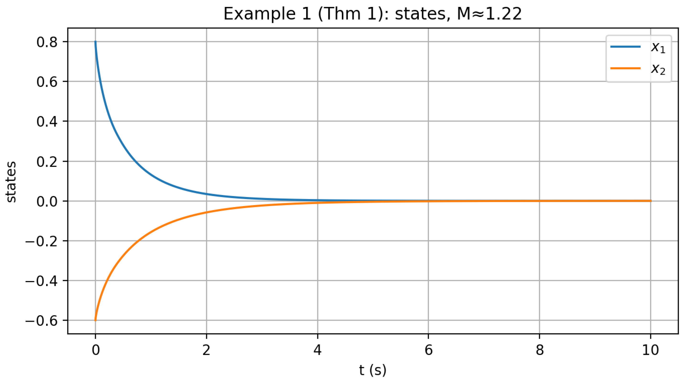
Figure 2.
Practical stability under bounded disturbance (Example 2). The dashed lines indicate the ultimate bound .
Figure 2.
Practical stability under bounded disturbance (Example 2). The dashed lines indicate the ultimate bound .
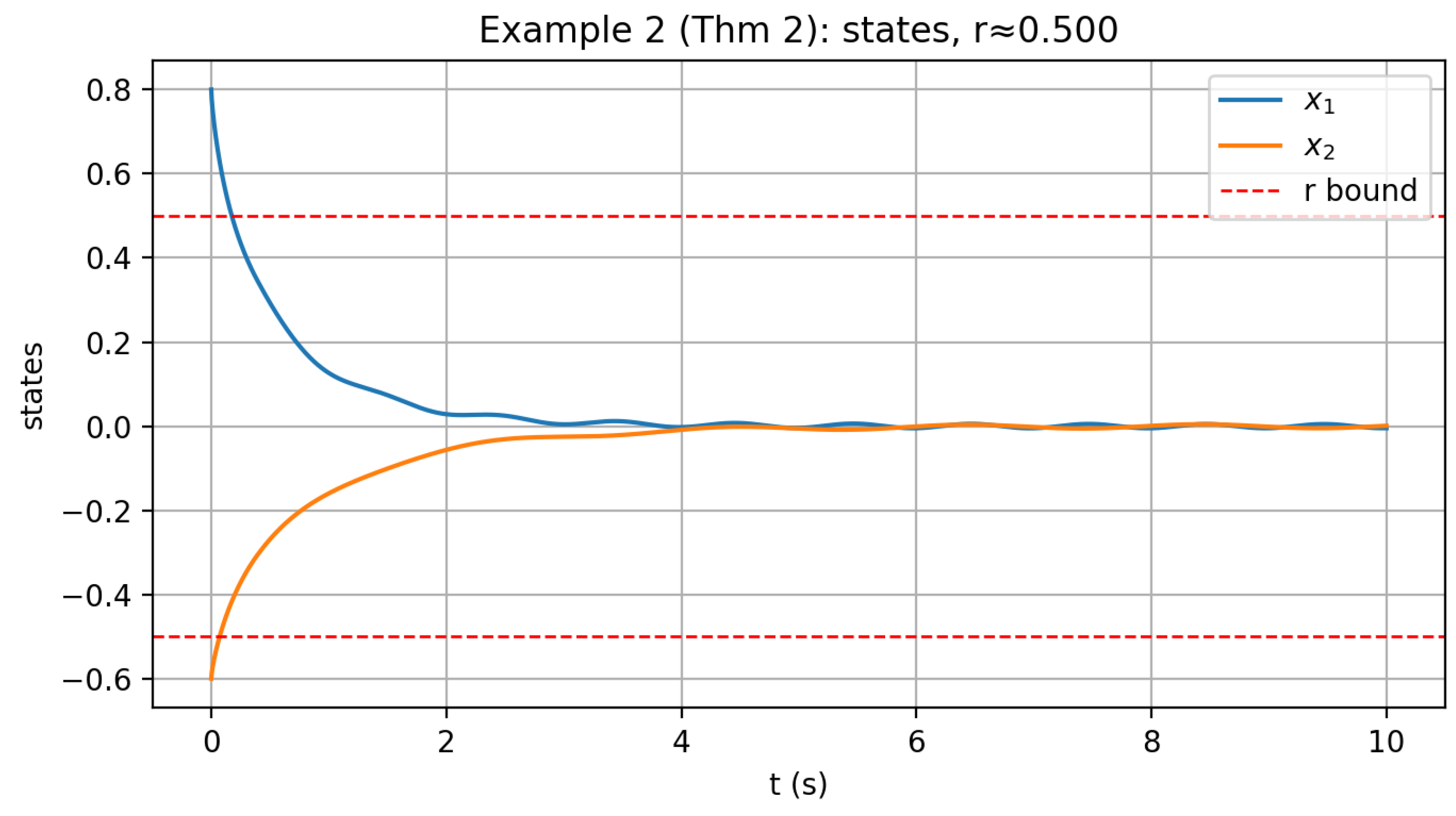
Figure 3.
Closed-loop stabilization: states (top) and control inputs (bottom) for Example 3.
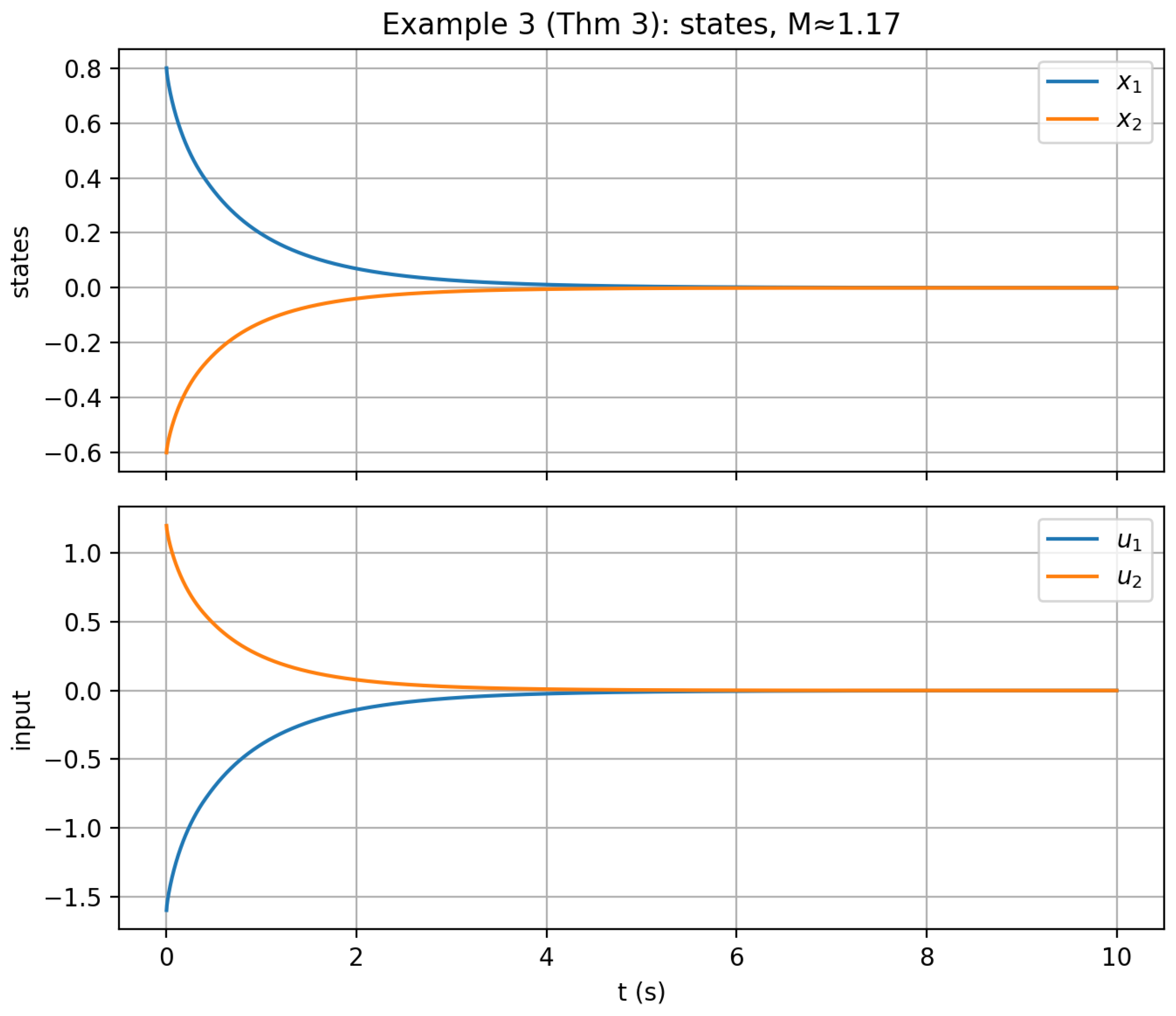
Figure 4.
Practical stabilization under disturbance: states (top) and control inputs (bottom) for Example 4. The dashed lines indicate the ultimate bound .
Figure 4.
Practical stabilization under disturbance: states (top) and control inputs (bottom) for Example 4. The dashed lines indicate the ultimate bound .
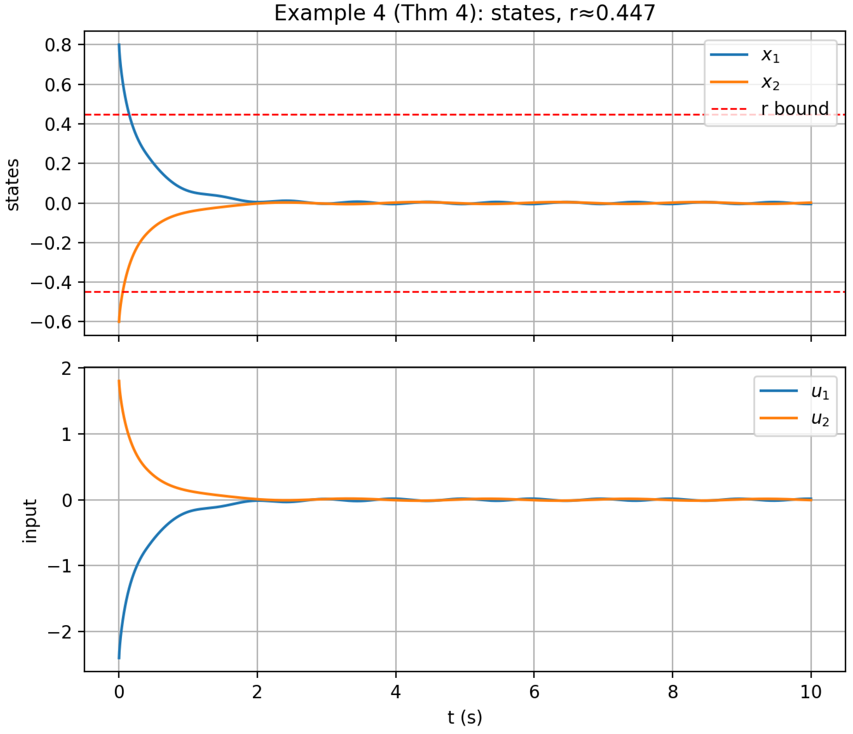

Table 1.
Comparison of representative LMI-based results for (conformable/fractional) nonlinear systems with/without time delay.
Table 1.
Comparison of representative LMI-based results for (conformable/fractional) nonlinear systems with/without time delay.
| Work | Class | Delay | Main result | Convex | Exp. rate/r | Robust | Notes |
|---|---|---|---|---|---|---|---|
| Naifar et al. (2018) [18] | Frac. (Mittag–Leffler), nonlin. | No | Practical ML stabilization (output feedback) | — | ML-type bound | — | Fractional stabilization; not in OSL/QIB; no explicit delay. |
| Ben Makhlouf & Naifar (2023) [19] | Gen. conformable (analysis) | No | Barbalat-type lemma; observer/analysis tools | — | — | — | Analytical foundations; not a control synthesis result. |
| Kharrat et al. (2023) [17] | Conformable (nonlin.) | Yes | Practical stability via LKF | Yes (LMIs) | r (explicit) | — | Conformable + delay; OSL/QIB not explicitly exploited. |
| Aldandani et al. (2023) [16] | Gen. conformable | No (as posed) | Practical stability (generalized conformable) | Yes (LMIs) | r (explicit) | — | Conformable setting; no explicit OSL/QIB structure; no explicit delay. |
| Iben Ammar et al. (2024) [20] | Conformable T–S fuzzy | Yes | Stability & stabilization (polynomial fuzzy) | Yes (LMIs) | — | — | Different nonlinearity class (T–S fuzzy); not focused on OSL/QIB. |
| This paper | OSL+QIB, conformable | Yes | Exponential & practical stability; state-feedback stabilization | Yes (LMIs) | Explicit & r | Yes | Convex LMIs; explicit decay and ultimate bound r; implementable algorithms; first to combine OSL+QIB with conformable derivative and delay to deliver exponential/practical stability and convex synthesis. |
Abbrev. Frac.=fractional; nonlin.=nonlinear; T–S=Takahgi–Sugeno; ML=Mittag–Leffler. “Convex” refers to LMI-based feasibility/synthesis; “r” denotes an explicit ultimate bound; “—” = not reported/applicable.
Disclaimer/Publisher’s Note: The statements, opinions and data contained in all publications are solely those of the individual author(s) and contributor(s) and not of MDPI and/or the editor(s). MDPI and/or the editor(s) disclaim responsibility for any injury to people or property resulting from any ideas, methods, instructions or products referred to in the content. |
© 2025 by the authors. Licensee MDPI, Basel, Switzerland. This article is an open access article distributed under the terms and conditions of the Creative Commons Attribution (CC BY) license (http://creativecommons.org/licenses/by/4.0/).
Copyright: This open access article is published under a Creative Commons CC BY 4.0 license, which permit the free download, distribution, and reuse, provided that the author and preprint are cited in any reuse.


