
Submitted:
20 December 2024
Posted:
23 December 2024
You are already at the latest version
Abstract
The Euler-Type Universal Numerical Integrator (E-TUNI) is a discrete numerical structure that couples a first-order Euler-type numerical integrator with some feed-forward neural network architecture. Thus, E-TUNI can be used to model non-linear dynamic systems when the real-world plant’s analytical model is unknown. From the discrete solution provided by E-TUNI, the integration process can be either forward or backward. Thus, in this article, we intend to use E-TUNI in a backward integration framework to model autonomous non-linear dynamic systems. Three case studies, including the dynamics of the non-linear inverted pendulum, were developed to verify the computational and numerical validation of the proposed model.
Keywords:
Universal Numerical Integrator (UNI)
; Nonlinear Auto Regressive Moving Average with eXogenous inputs (NARMAX)
; neural differential equations
; Euler-Type Universal Numerical Integrator (E-TUNI)
; Runge-Kutta Neural Network (RKNN)
; Adams-Bashforth Neural Network (ABNN)
1. Introduction
The Euler-Type Universal Numerical Integrator (E-TUNI) is a particular case of a Universal Numerical Integrator (UNI). In turn, the UNI is the coupling of a conventional numerical integrator (e.g., Euler, Runge-Kutta, Adams-Bashforth, Predictive-Corrector, among others) with some kind of universal approximator of functions (e.g., MLP neural networks, SVM, RBF, wavelets, fuzzy inference systems, among others). Furthermore, UNIs generally work exclusively with neural networks with feed-forward architecture through supervised learning with input/output patterns.
In [1], the first work involving the mathematical modeling of an artificial neuron is presented. In [2,3], it is mathematically demonstrated, independently, that feed-forward neural networks with Multi-Layer Perceptron (MLP) architecture are universal approximators of functions. For the mathematical demonstration of the universality of feed-forward networks, a crucial starting point is the Stone-Weierstrass theorem [4]. An interesting work on the universality of neural networks involving the ReLU neuron can be found in [5]. In summary, many neural architectures were developed in the last half of the twentieth century, involving shallow neural networks [6]. On the other hand, in this century, many architectures of deep neural networks demonstrated the great power of neural networks [7].
So, artificial neural networks solve an extensive range of computational problems. However, in this article, we limit the application of artificial neural networks with feed-forward architecture in the resolution of mathematical problems involving modeling autonomous non-linear dynamic systems governed by a system of ordinary differential equations. With the neural networks, it is possible to solve the inverse problem of modeling dynamical systems, that is, given the solution of the dynamical system, then obtain the instantaneous derivative functions or the mean derivative functions of the system.
The starting point for the proper design of a Universal Numerical Integrator (UNI) is the conventional numerical integrators [8,9,10,11,12,13,14,15]. In [16], a qualitative and very detailed description of the design of a UNI is presented. Also, in [16], an appropriate classification is given for the various types of Universal Numerical Integrators (UNIs) found in the literature.
According to these authors, the UNIs can be divided into three large groups, giving rise to three different methodologies, namely: (i) the NARMAX methodology (Nonlinear Auto Regressive Moving Average with Exogenous input); (ii) the instantaneous derivatives methodology (e.g., Runge-Kutta neural network, Adams-Bashforth neural network, Predictive-Corrector neural network, among others), and (iii) mean derivatives methodologies or E-TUNI. For a detailed understanding of the similarities and differences between the existing UNIS types, see again [16].
In practice, the leading scientific works involving the proper design of a UNI are: (i) the NARMAX methodology in [17,18,19,20,21]; (ii) the Runge-Kutta neural network in [22,23,24,25]; (iii) the Adams-Bashforth neural network in [26,27,28]; and (iv) the E-TUNI in [29,30,31,32,33,34]. For this article, it should be noticed that E-TUNI works exclusively with mean derivative functions instead of instantaneous derivative functions. Furthermore, the NARMAX and mean derivative methodologies are of fixed steps in the simulation phase, while the instantaneous derivative methodologies are of varied integration steps in the simulation phase [16]. However, all of them are fixed steps in the training phase.
In this paragraph, we briefly describe existing work on E-TUNI. In [29], the doctoral thesis gave rise to E-TUNI. In [30], it is a technological application of E-TUNI using neural networks with MLP architecture. In [32], it is a technological application of E-TUNI using fuzzy logic and genetic algorithms. Still in [32], the fuzzy membership functions are adjusted automatically, using genetic algorithms through supervised learning using input/output patterns. In [34], E-TUNI is designed with an MLP neural architecture and later applied in a predictive control structure.
However, none of the previous works used E-TUNI with backward integration. Therefore, this article’s originality lies in using E-TUNI in a backward integration process coupled with a shallow neural network with MLP architecture. As far as we know, this has not yet been done.
This article is divided as follows: Section 2 briefly describes the basic structure of a Universal Numerical Integrator (UNI). Section 3 describes the detailed mathematical development of E-TUNI, designed with backward integration. Section 4 presents the numerical and computational results validating the proposed model. Section 5 presents the main conclusions of this work.
2. Universal Numerical Integrator (UNI)
Figure 1 illustrates a general scheme for adequately designing a Universal Numerical Integrator (UNI). Notice that in Figure 1, when one couples a conventional numerical integrator (e.g., Euler, Runge-Kutta, Adams-Bashforth, predictive-corrector, among others) to some kind of universal approximators of functions (e.g., MLP neural networks, RBF, SVM, fuzzy inference systems, among others), the UNI design can be achieved high numerical accuracy through supervised learning using input/output training patterns. This allows for solving real-world problems involving the modeling of non-linear dynamic systems.
As previously mentioned, a Universal Numerical Integrator (UNI) can be of three types, thus giving rise to three distinct methodologies, namely: (i) NARMAX model, (ii) instantaneous derivatives methodology (e.g., Runge-Kutta neural network, Adams-Bashforth neural network, predicted-corrector neural network, among others), and (iii) mean derivatives methodology or E-TUNI. The three types of universal numerical integrators are equally precise, as the Artificial Neural Network (ANN) is a universal approximator of functions [2,3,4,5], every UNI can have its approximation error as close to zero, as much as one likes.
To fully understand the difference between the instantaneous and the mean derivatives methodologies, see Figure 2. Figure 2 also presents the geometric difference between the instantaneous and mean derivatives functions. Everyone knows that the mean derivative is the secant line between two distinct points of any mathematical function. The instantaneous derivative is the tangent line to any point of a mathematical function.
The mean derivatives methodology occurs when a universal approximator of functions is coupled to the Euler-type first-order integrator. In this case, the first-order integrator would have a substantial error if instantaneous derivative functions were used. However, when the mean derivative functions replace the instantaneous derivative functions, the integrator error is reduced to zero [16,30,31]. In this way, it is possible to train an artificial neural network to learn the mean derivative functions through two possible approaches [16]: (i) the direct approach and (ii) the indirect or empirical approach.
Figure 3 schematically represents the direct approach. Figure 4 schematically represents the indirect or empirical approach. In the direct approach, the artificial neural network is trained separately from the first-order integrator. The artificial neural network is trained and coupled to the first-order integrator in the indirect or empirical approach. Both approaches are equivalent to each other. However, the back-propagation algorithm must be recalculated using the indirect or empirical approach. In the direct approach, this is unnecessary [16,29].
This difference between the direct and indirect approach also applies to the instantaneous derivatives methodology. However, in this case, the direct approach only applies to theoretical models, as instantaneous derivative functions cannot be determined directly in real-world problems [16]. Furthermore, this difference between the direct and indirect approach does not apply to the NARMAX model. However, the NARMAX model is also a particular case of UNI. This is because, although a conventional integrator is not coupled to the NARMAX model, the universal approximator of functions behaves as if it were a numerical integrator [16].
3. The Euler-Type Universal Numerical Integrator (E-TUNI)
The equation (1) mathematically represents a system of n autonomous non-linear ordinary differential equations with dependent variables . Based on this, it is possible to establish an initial value problem for a first-order system, also described by (1).
The solution of the differential equation (1) can be obtained through a first-order approximation. Such a solution was obtained by the mathematician Leonard Euler in 1768. This solution, keeping the convention described by Figure 2, is given by the equation (2).
However, everyone knows that the accuracy of the equation (2) is awful. Because of this, if the instantaneous derivative functions are replaced by the mean derivative functions, then the Euler-type first-order integrator becomes precise [16,29,31]. This new solution is given by equation (3).
Notice that the equation (3) is straightforward to obtain, as the mean derivative functions sound easily computable, for real-world problems, via equation (4), for . Here, the variable n is the total number of state variables of the dynamical system given by (1).
It is crucial to notice that a neural network can compute the mean derivative functions, as schematized by Figure 5. In this way, the E-TUNI works with a first-order numerical integrator coupled to a neural network with any feed-forward architecture (e.g., MLP neural network, RBF, SVM, wavelets, fuzzy inference systems, Convolutional Neural Network (CNN), among others).
3.1. The E-TUNI with Backward Integration
Let be the autonomous system of nonlinear differential equations
where, e .
By definition, let also be for a trajectory about the family of solutions of the non-linear differential equations system that passes through at the initial instant . Here, the index j indicates the variable’s name, and is the number of discretizations of the initial condition that can be as large as one likes. So, the Theorem 1 (T1) is very important, as it deals with the uniqueness of the solutions of the differential equation (5).
Theorem 1 (T1). Assume that each of the functions has continuous partial derivatives with respect to . So the known initial value problem for has one and only one solution in , starting from each . If two solutions have a common point, they must be identical.
Theorem 2 (The Differential Mean Value Theorem): If a function for is a continuous function and defined over the closed interval is differentiable over the open interval , then there exists at least one number with such that, .
Theorem 3 (The Mean Integral Value Theorem): If a function for is a continuous function and defined over the closed interval , then there exists at least one internal point in such that, .
In general, as has no analytic solution, then it is expected to know for just a discrete set of points to at the horizon and a constant; thus, the vector in question is a piece of a discrete solution to , where
By definition [35,36], the secant between two points and for belonging to the curve is the line segment joining these two points. Then, the tangents of the secants between the points and for are defined as:
where, , for .
The variable is the angle of the secant that joins the two points and belonging to the curve . Thus, it is possible to demonstrate Theorem 4 (T4) concerning the solution of the dynamical system governed by autonomous non-linear ordinary differential equations [37].
Theorem 4 (T4). The solution for of the nonlinear differential equations system can be determined exactly through the relation for a given e .
Proof. It is presented in detail in [29,37]. However, there is an error in the proof of this theorem in [29], which was corrected in [37]. Additionally, we can provide some simplified proof here. When the general solution of the nonlinear autonomous dynamical system is known, then can be replaced by some function of the type . This allows us to apply systematically and recursively theorems T2 and T3 to the original differential equation (1) and easily arrive at the desired proof. Because of the Uniqueness Theorem T1, there is no other mathematical form than this one. In an approach involving supervised learning of input/output training patterns, knowing the solution one wants to arrive at in advance is not absurd.
Therefore, it is important to mathematically relate the mean derivatives functions with the instantaneous derivatives functions (see again Figure 2). Thus, it is easily seen that if then,
or
Figure 2 graphically illustrates the convergence of mean derivatives functions to instantaneous derivatives functions when tends to zero. Based on this, it is possible to enunciate two basic types of first-order numerical integrators or Euler integrators. An Euler integrator that uses instantaneous derivatives functions, given by for and an Euler integrator that uses mean derivatives functions, given by .
A significant difference between the mean derivatives functions and the instantaneous derivatives functions is that the instantaneous derivatives functions for is only dependent on , but the mean derivatives functions for is dependent on , and at the point . As will be seen later, this difference is significant.
The first important point to be considered here is the possibility of carrying out both forward and backward integration of the Euler Integrator with instantaneous derivatives. So, the instantaneous derivative functions at the points for can be defined in two different ways:
or
However, if the instantaneous derivatives functions exists at the point , then necessarily or (see Figure 6). In this way, the expressions of forward and backward propagating Euler integrators, necessarily designed with the instantaneous derivative functions, are given, respectively, by (i.e., with low numerical precision):
Notice that the equation (13) can also be obtained directly from the equation (12) by making the substitution of the variable .
Additionally, like , the Euler integrator with instantaneous derivatives functions has a symmetric solution between intervals and , thus implying low numerical precision, for the outputs and for . To say that a solution is symmetric at the point k means to say that to .
This Euler integrator symmetry property only occurs when instantaneous derivative functions are used. However, in Euler’s integrator, designed with the mean derivatives functions, this symmetry of the solution around the point is not verified (see Figure 6 again). This is important because in Euler’s integrator, designed with mean derivatives functions, the backward solution does not necessarily decrease when the forward solution grows.
In [38], several difference operators can be applied to a function for . However, the two operators that interest us are the forward difference and the backward difference, given below, respectively:
Thus, using the finite difference operators, there are two different ways to represent the secant at the point and with integration step :
Comparing the equation (16) with the result of Theorem T4, one can obtain the following recursive and exact equation to represent the solution of autonomous non-linear ordinary differential equations system for a forward integration process (i.e., with high numerical accuracy):
or
Equations (18) and (19) represent an Euler-type integrator, which uses mean derivatives functions and forward integration. However, to obtain the Euler integrator with backward recursion, it is enough to analyze the asymmetry of the mean derivative functions at the point and as illustrated in Figure 6. In this way, we can obtain the following equation to perform the backward integration of E-TUNI (i.e., with high numerical precision):
or
Thus, the iterative equations of the first-order Euler integrator, using mean derivatives, which perform forward and backward recursions, are, respectively, equations (18) and (20). The negative sign that appears in the equation (20) means, not necessarily, that when increases, then decreases, because they are two neural networks independent of each other. Therefore, it is observed that, in general, , and therefore Euler integrators with mean derivatives functions do not have a symmetric solution, that is, in general, for . As can be easily seen in Figure 6, the negative mean derivative has a different slope than the positive mean derivative for the same point in .
4. Results and Analysis
In this section, we perform a numerical and computational analysis of the Universal Numerical Integrator (UNI), which exclusively uses mean derivative functions. As previously described, this is the Euler-Type Universal Numerical Integrator (E-TUNI). Therefore, we present here three case studies: (i) a one-dimensional simple case, (ii) the non-linear simple pendulum (two state variables), and (ii) the non-linear inverted pendulum (four state variables).
Thus, for all experiments that it is presented below, the use of MLP neural networks was standardized with the traditional Levenberg-Marquardt training algorithm [39] from 1994. Concerning the architecture of the neural network used, all experiments were trained using only one inner layer (with thirty neurons with tangent hyperbolic activation function) in an artificial neural network of the Multi-Layer Perceptron (MLP) type. In all experiments, of the total patterns were left for training the MLP neural network, of the patterns for testing, and for validation. Concerning the architecture of E-TUNI, the direct approach was exclusively used. However, it must be said that the indirect or empirical approach of E-TUNI was not tested in this article. Thus, the general algorithm for training and testing the methodology presented in this article can be briefly described as follows:
Step 1. Using a high-order 4-5 Runge-Kutta integrator, over the considered autonomous non-linear ordinary differential equation system, randomly generate p training patterns input/output for E-TUNI concerning the initial instant . Perform both forward and backward integration.
Step 2. Determine both the values of the positive mean derivatives , as well as the values of the negative mean derivatives in relation to initial instants for .
Step 3. Train two distinct neural networks. One is to output positive mean derivative functions, and the other is to output negative mean derivative functions. Do this following the graphic diagram in Figure 5.
Step 4. Simulate, for several different integration steps, the performance of E-TUNI both with forward and backward integration. Observe that if starting from an initial instant , the solution is propagated in n distinct instants forward and, after that, one returns to the same n instants with backward integration because of the uniqueness theorem, one returns perfectly to the original initial instant . This trick will be used to test the efficiency of E-TUNI when it is propagated backward.
Step 5. Do the same, using the Euler-type first-order integrator, but now using the original instantaneous derivative functions of the dynamical system in question. Then, compare E-TUNI with conventional Euler. Thus, to verify the superiority of E-TUNI concerning the conventional Euler, the accuracy of the discrete numerical solutions obtained must be verified.
Therefore, next, we briefly describe the systems of non-linear differential equations of the three dynamical systems considered here to test the proposed algorithm to perform the backward integration of E-TUNI. Table 1 also summarizes the training data of the eight experiments conducted here to test the proposed methodology.
Example 1. Simulate the one-dimensional non-linear dynamics problem, given by the equation (22). The variable y was trained on the range . Notice that this dynamic has infinite stability points since has infinitely many solutions. Notice that the points of stability recovering the initial condition through backward integration is very difficult for any integrator.
Example 2. Simulate the non-linear simple pendulum problem given by the system of differential equations (23). Notice that, this example does not involve control variables. The acceleration values due to gravity constants and the pendulum’s length are, respectively, given by and . The variable was trained on the range and the variable was trained on the range .
Example 3. Do the same for the non-linear inverted pendulum problem described by the system of differential equations (24). The constants adopted for this problem were , , , , , , e . This problem has four state variables (, , , and ) and a constant control (). The state variables were trained on the intervals between , between , between , and between .
Figure 7 graphically illustrates the numerical simulation obtained for Example 1. This figure is not yet the result obtained by E-TUNI, but by Runge-Kutta 4-5, available in Matlab, to numerically solve the equation (22). Therefore, the result obtained by E-TUNI will be compared later, numerically and graphically, with the graphic result of this figure. Also, in Figure 7, the following convention was used: (i) the blue dots in "x" represent the forward propagation, in high precision, of Runge-Kutta 4-5 over the dynamics of the equation (22), (ii) the blue dots in "o" represent the high precision backward propagation of Runge-Kutta 4-5 over the same dynamics, and (iii) the solid red lines represent the slope of the mean derivatives functions between two consecutive points.
Notice that the integration step, graphically presented, was . However, it is essential to notice that the Runge-Kutta 4-5 works internally with a varied integration step much smaller than this one to achieve the high numerical accuracy shown in Figure 7. So, both forward and backward integration were performed from to . In this case, as can be seen, the result obtained is perfect, as the points obtained by backward integration overlapped perfectly over the points with forward integration.
Figure 8 presents the first graphic result of E-TUNI, for the dynamics given by equation (22). The blue dots represent the results obtained by E-TUNI and follow the same convention as in the previous figure. The green dots represent the results obtained by the conventional Euler Integrator, using the instantaneous derivative functions, also given by the equation (22). The two black dash-dot horizontal lines delimit the E-TUNI training range. Notice that within the training range, the E-TUNI result was perfect, with both forward and backward integration. The line in Table 1 with the indicates the training data obtained for this case. In this way, 400 training patterns were generated, and of them, 320 patterns, were effectively left for training. Notice that in Table 1 the symbols and represent, respectively, the mean square error of forward integration and the mean square error of backward integration.
Notice that, outside the training region, E-TUNI has become inaccurate. However, to solve this problem, the training domain of the state variable should be increased. Notice also that the conventional Euler presented a slight deviation in the backward integration concerning the forward integration in the given domain. Thus, in conventional Euler, this deviation becomes more critical and accentuated, which increases the integration step. However, in E-TUNI, the result does not deteriorate with the increase of the integration step.
Figure 9 presents the same result as the previous figure, but now using an integration step . The E-TUNI result was perfect, but the conventional Euler result was even worse. This confirms what was said in the previous paragraph. See Table 1 again in line to find out about the main parameters used in this training. Figure 10 presents the same result as the previous figure, but now using an integration step . In this case, the result achieved by E-TUNI is still perfect, and the result by conventional Euler is as well. The result, obtained by conventional Euler, was perfect, in this case, because a tiny integration step was used and equal to . Figure 11 presents a simulation using the integration step . Again, E-TUNI presented a perfect result, but the conventional Euler degenerated its solution.
Figure 12 and Figure 13 deserve a little more attention. In Figure 12, as can be seen, the solution obtained by E-TUNI, through backward integration, was degenerate (see the zoom). In this case, the blue circle should lie perfectly on the solid red line. In Figure 13, the backward integration solution obtained by Runge-Kutta 4-5 was also degenerate. Both solutions turned out bad because the integration process was conducted for too long, over a point of stability. The zoom made in Figure 12 will be used to better explain this.
What is explained for Figure 12 is also valid for Figure 13. In Figure 12, the integration process was conducted from to . The biggest problem occurred when returning from to . For example, all families of curves confined between and at the initial instant were confined in a much smaller interval than this one at the instant . Therefore, to work properly, backward integration would have to be trained with a much smaller mean squared error than the one achieved in Table 1 (line ). However, this is impossible to achieve using just the algorithm in [39]. Notice that this task was also impossible for Runge-Kutta 4-5, as schematized in Figure 13. Therefore, the problem presented here is critical, regardless of the integrator used.
Figure 14 presents the first graphic result of E-TUNI for the dynamics given by the equation (23), which represents the dynamics of the non-linear simple pendulum. In this case, the superiority of E-TUNI over the conventional Euler is evident. An integration step was used in this case. Figure 15 concerns the same previous example, but using an integration step . The conventional Euler was not presented in this figure because its result was awful, which would impair, therefore, the scale of the graph. Still referring to Figure 15, the main reason the backward integration turned out to be a bit bad at the end of the integration process is that the average training error became slightly oversized (see Table 1 in cell ). To solve this problem, it is enough to reduce the average training error of the artificial neural network used, but that is not always an easy task. Figure 16 demonstrates that, even for Runge-Kutta 4-5, the backward integration process of the simple pendulum can also be imperfect (see blue circles misaligned with the blue "x").
Notice that the solution from equation (23), graphically presented in Figure 15, was much worse than the other solutions given in Table 1. This fact can be seen by checking the training mean square errors in Table 1 (line ), which were too high. Most likely, this was caused by two fundamental reasons. The first reason is that the E-TUNI local error is amplified by the square of the Integration step (see columns 7 and 9 of Table 1). The proof of this result can be found in [29] or in [37]. However, the analysis of the global error would require further studies. The other reason, which is purely speculative, is the following: it is believed that when the E-TUNI integration step is very large if the solution of the real dynamical system becomes a non-convex function (concerning the line of mean derivatives in this same interval ), then the training becomes more difficult. However, this last argument still needs to be verified empirically and theoretically.
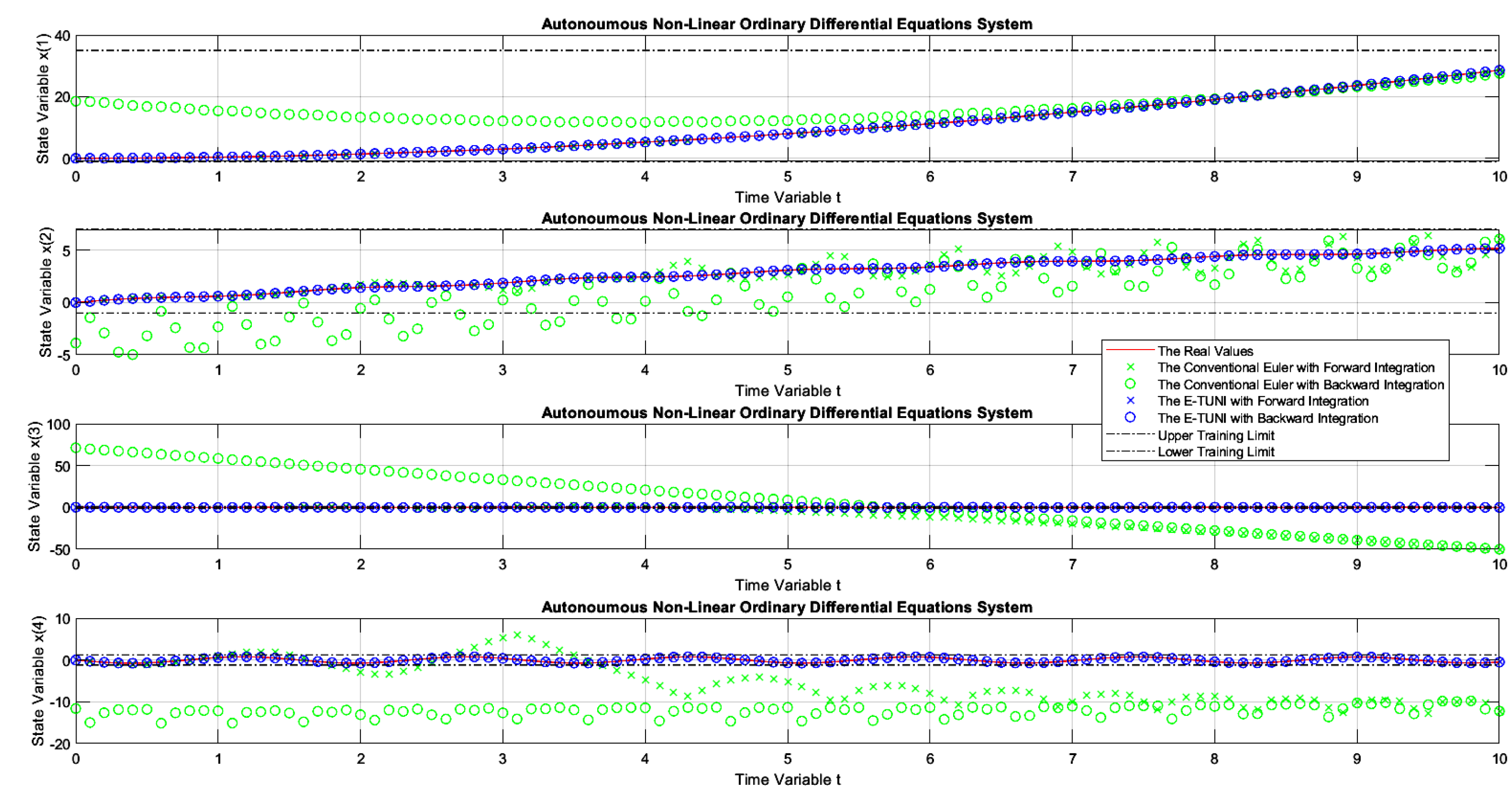
Figure 17 presents the first graphic result of E-TUNI, for the dynamics given by the equation (24), which represents the dynamics of the non-linear inverted pendulum. As can be seen, in this figure, Runge-Kutta 4-5 perfectly simulated this dynamic, both for forward and backward integrations. Figure 18 is the same case simulation but performed by E-TUNI. Theoretically, Figure 18 is the same as Figure 17. They are just on different scales. Notice that in Figure 18 the E-TUNI simulation was perfect. However, the conventional Euler simulation (green dots) became confusing due to the numerical imprecision achieved by it. Furthermore, this caused an exaggerated change in the scale of the figure.

5. Conclusion
As far as we know, all previous work on E-TUNI was developed using only forward integration. Therefore, we present here, for the first time, a work that uses E-TUNI in a backward integration process. Three case studies were carried out. Non-linear and autonomous ordinary differential equations govern all three dynamical systems considered in this study.
The Euler-type Integrator designed with instantaneous derivatives is not very accurate. However, the E-TUNI has numerical precision equivalent to that of the highest-order integrators. It is interesting to notice that the elegance of the theory of ordinary differential equations can be improved when combined with the theory of universal approximator of functions. This propriety is possible because artificial neural networks allow working with real-world input/output training patterns. This fact enables refining the final solution obtained by the first-order Euler integrator and estimator. Because of this, the E-TUNI can also be used to predict real-world dynamics (e.g., river flow and stock market forecasts, among others).
Additionally, we can call the forward mean derivatives functions positive mean derivatives functions. Equivalently, we can call the backward mean derivatives functions negative mean derivatives functions. Thus, we also conclude that the mean derivative functions depend on the integration step and are asymmetric. This propriety means training two distinct neural networks to simultaneously perform forward and backward integration. Unfortunately, the positive and negative instantaneous derivative functions are symmetric to each other.
Finally, it would be interesting to carry out a future study of E-TUNI using deep neural networks instead of shallow neural networks, aiming to reach two essential points: (i) to be able to increase the number of training patterns (and, consequently, the domain of state variables) and (ii) try to reduce the training mean squared error, as this quantity is critical, in the case of modeling non-linear dynamic systems designed through artificial neural networks. Interestingly, E-TUNI is an excellent option to replace the NARMAX model and even the Runge-Kutta Neural Network (RKNN).
Author Contributions
P.T. designed the proposed model and wrote the main part of the mathematical model. J. M., L.D., and A.C. supervised the writing of the paper and its technical and grammatical review. P.T. and G.G. (supervised by J. M., L.D., and A.C.) developed the software and performed several computer simulations to validate the proposed model.
Funding
The authors thank the Brazilian Aeronautics Institute of Technology (Instituto Tecnológico de Aeronáutica - ITA); the Casimiro Montenegro Filho Foundation (Fundação Casimiro Montenegro Filho - FCMF); and the Brazilian Enterprise Ecossistema Negócios Digitais Ltda for their support and infrastructure, which motivate the challenges and innovations of this research project.
Institutional Review Board Statement
Not applicable.
Informed Consent Statement
Not applicable.
Data Availability Statement
Not applicable.
Acknowledgments
I would like to thank Professor and great friend Atair Rios Neto for his valuable tips for improving this article. Finally, I would also like to thank the valuable improvement tips given by the good reviewers of this journal. The authors of this article would also like to thank God for making all of this possible.
Conflicts of Interest
The authors declare no conflict of interest.
Abbreviations
The following abbreviations are used in this manuscript:
| ABNN | Adams-Bashforth Neural Network |
| E-TUNI | Euler-Type Universal Numerical Integrator |
| L-MTA | Levenberg-Marquardt Training Algorithm |
| MSE | Mean Square Error |
| MLP | Multi-Layer Perceptron |
| NARMAX | Nonlinear Auto Regressive Moving Average with eXogenous inputs |
| PCNN | Predictive-Corrector Neural Network |
| RBF | Radial Basis Function |
| RKNN | Runge-Kutta Neural Network |
| SVM | Support Vector Machine |
| UNI | Universal Numerical Integrator |
References
- McCulloch, W.; Pitts, W. A logical calculus of the ideas immanent in nervous activity. Bull. Math. Biol. 1943, 5(6), 115–133. [CrossRef]
- Cybenko, G. Approximation by superpositions of a sigmoidal function. Math. Control. Signals, Syst. 1989, 2(4), 303–314. [CrossRef]
- Hornik, K.; Stinchcombe, M.; White, H. Multilayer feedforward networks are universal approximators. Neural Netw. 1989, 2(5), 359–366. [CrossRef]
- Cotter, N. E. The Stone-Weierstrass and its application to neural networks. IEEE Trans. Neural Netw. 1990, 1(4), 290–295. [CrossRef]
- Hanin, B. Universal function approximation by deep neural nets with bounded width and ReLU activations. Mathematics 2019, 7(10), 1–9. [CrossRef]
- Haykin, S. Neural Networks: A Comprehensive Foundation. Publisher: Prentice-Hall, Inc., New Jersey, USA, 1999.
- Goodfellow, I.; Bengio, Y.; Courville, A. Deep Learning. Publisher: MIT Press, Cambridge, MA, 2017.
- Henrici, P. Elements of Numerical Analysis. Publisher: John Wiley and Sons, New York, USA, 1964.
- Lapidus, L.; Seinfeld, J. H. Numerical Solution of Ordinary Differential Equations. Publisher: Academic Press, New York and London, 1971.
- Lambert, J. D. Computational Methods in Ordinary Differential Equations. Publisher: John Wiley and Sons, New York, USA, 1973.
- Vidyasagar, M. Nonlinear Systems Analysis. Publisher: Prentice-Hall, Inc., Electrical Engineering Series, New Jersey, USA, 1978. [CrossRef]
- Chen, D. J. L.; Chang, J. C.; Cheng, C. H. Higher order composition Runge-Kutta methods. Tamkang Journal of Mathematics 2008, 39(3), 199–211. [CrossRef]
- Misirli, E.; Gurefe, Y. Multiplicative Adams Bashforth-Moulton methods. Numer. Algor. 2011, 57(4), 425–439. [CrossRef]
- Ming, Q.; Yang, Y.; Fang, Y. An optimized Runge-Kutta method for the numerical solution of the radial Schrödinger equation. Mathematical Problems in Engineering 2012, 2012(1), 1–12. [CrossRef]
- Polla, G. Comparing accuracy of differential equation results between Runge-Kutta Fehlberg methods and Adams-Moulton methods. Applied Mathematical Sciences 2013, 7(103), 5115–5127. [CrossRef]
- Tasinaffo, P. M.; Gonçalves, G. S.; Cunha, A. M.; Dias, L. A. V. An introduction to universal numerical integrators. Int. J. Innov. Comput. Inf. Control 2019, 15(1), 383–406. [CrossRef]
- Chen, S.; Billings, S. A. Representations of nonlinear systems: the NARMAX model. Int. J. Control 1989, 49(3), 1013–1032. https://api.semanticscholar.org/CorpusID:122070021.
- Chen, S.; Billings, S. A.; Cowan, C. F. N.; Grant, P. M. Practical identification of NARMAX models using radial basis functions. Int. J. Control 1990, 52(6), 1327–1350. https://api.semanticscholar.org/CorpusID:16430646.
- Narendra, K. S.; Parthasarathy, K. Identification and control of dynamical systems using neural networks. IEEE Trans. Neural Netw. 1990, 1(1), 4–27. [CrossRef]
- Hunt, K. J.; Sbarbaro, D.; Zbikowski, R.; Gawthrop, P. J. Neural networks for control systems – A survey. Automatica 1992, 28(6), 1083–1112. https://api.semanticscholar.org/CorpusID:207511431.
- Norgaard, M.; Ravn, O.; Poulsen, N. K.; Hansen, L. K. Neural Networks for Modelling and Control of Dynamic Systems. Publisher: Springer, London, UK, 2000. https://link.springer.com/book/9781852332273.
- Wang, Y.-J.; Lin, C.-T. Runge-Kutta neural network for identification of dynamical systems in high accuracy. IEEE Trans. Neural Netw. 1998, 9(2), 294–307. [CrossRef]
- Uçak, K. A Runge-Kutta neural network-based control method for nonlinear MIMO systems. soft Computing 2019, 23(17), 7769–7803. [CrossRef]
- Uçak, K.; Günel, G. O. An adaptive state feedback controller based on SVR for nonlinear systems. In Proceedings of the 6th International Conference on Control Engineering and Information Technology (CEIT), Istanbul, Turkey, 2018, 25–27. https://api.semanticscholar.org/CorpusID:195775331.
- Uçak, K. A novel model predictive Runge-Kutta neural network controller for nonlinear MIMO systems. Neural Processing Letters 2020, 51(2), 1789–1833. [CrossRef]
- Rios Neto, A.; Tasinaffo, P. M. Feedforward neural networks combined with a numerical integrator structure for dynamic systems modeling. In Proceedings of the 17th International Congress of Mechanical Engineering (COBEM), São Paulo/SP, Brazil, 2003,1–7.
- Melo,R. P.; Tasinaffo, P. M. Uma metodologia de modelagem empírica utilizando o integrador neural de múltiplos passos do tipo Adams-Bashforth. Sociedade Brasileira de Automática (SBA) 2010, 21(5), 487–509. [CrossRef]
- Tasinaffo, P. M.; Rios Neto, A. Adams-Bashforth neural networks applied in a predictive control structure with only one horizon. Int. J. Innov. Comput. Inf. Control 2019, 15(2), 445–464. [CrossRef]
- Tasinaffo, P. M. Estruturas de Integração Neural Feedforward Testadas em Problemas de Controle Preditivo. Doctoral Thesis, INPE-10475-TDI/945, São José dos Campos/SP, Brazil, 2003. http://urlib.net/sid.inpe.br/jeferson/2004/02.18.14.07.
- Tasinaffo, P. M.; Rios Neto, A. Mean derivatives based neural Euler integrator for nonlinear dynamic systems modeling. Learning and Nonlinear Models 2005, 3(2), 98–109.
- Tasinaffo, P. M.; Guimarães, R. S.; Dias, L. A. V.; Strafacci Júnior, V. Discrete and exact general solution for nonlinear autonomous ordinary differential equations. Int. J. Innov. Comput. Inf. Control. 2016, 12(5), 1703–1719. [CrossRef]
- de Figueiredo, M. O.; Tasinaffo, P. M.; Dias, L. A. V. Modeling autonomous nonlinear dynamic systems using mean derivatives, fuzzy logic and genetic algorithms. Int. J. Innov. Comput. Inf. Control 2016, 12(5), 1721–1743. [CrossRef]
- Tasinaffo, P. M.; Guimarães, R. S.; Dias, L. A. V.; Strafacci Júnior, V. Mean derivatives methodology by using Euler integrator improved to allow the variation in the size of integration step. Int. J. Innov. Comput. Inf. Control. 2016, 12(6), 1881–1891. [CrossRef]
- Tasinaffo, P. M.; Rios Neto, A.Predictive control with mean derivative based neural Euler integrator dynamic model. Sociedade Brasileira de Automática (SBA) 2006, 18(1), 94–105. [CrossRef]
- Munem, M. A.; Foulis, D. J. Calculus with Analytic Geometry (Volumes I and II). Publisher: Worth Publishers, Inc., New York, USA, 1978.
- Wilson, E. Advanced Calculus. Publisher: Dover Publication, New York, USA, 1958.
- Tasinaffo, P. M.; Dias, L. A. V.; da Cunha A. M. A Quantitative Approach to Universal Numerical Integrators (UNIs) with Computational Application. Human-Centric Intelligent Systems (preprint) 2024, 4, 1–20.
- Ames, W. F. Numerical Methods for Partial Differential Equations. Publisher: Academic Press, 2. ed., New York, USA, 1988.
- Hagan, M. T.; Menhaj, M. B. Training feedforward networks with the Marquardt algorithm. IEEE Trans. Neural Netw. 1994, 5(6), 989–993. [CrossRef]
Figure 1.
General graphic diagram of the operation of a Universal Numerical Integrator (UNI) (Source: [16,29]).
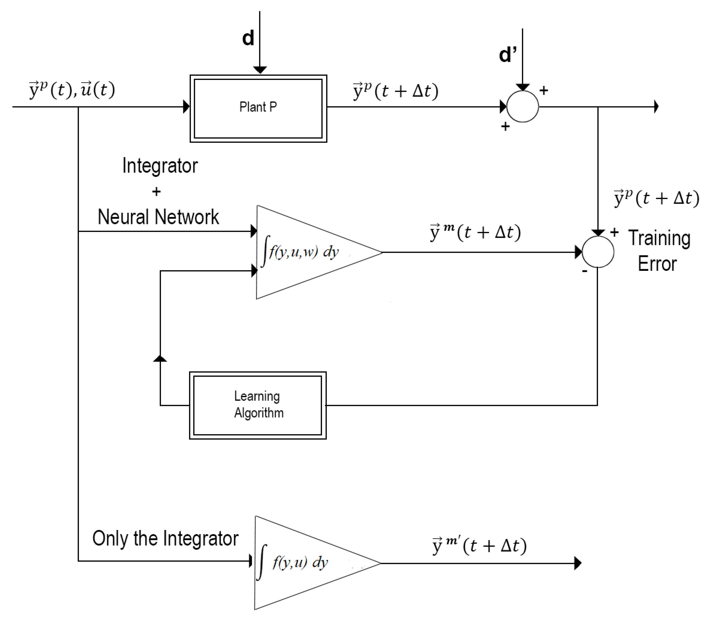
Figure 2.
Basic difference between the instantaneous derivative and the mean derivative (Source: [16,29]).
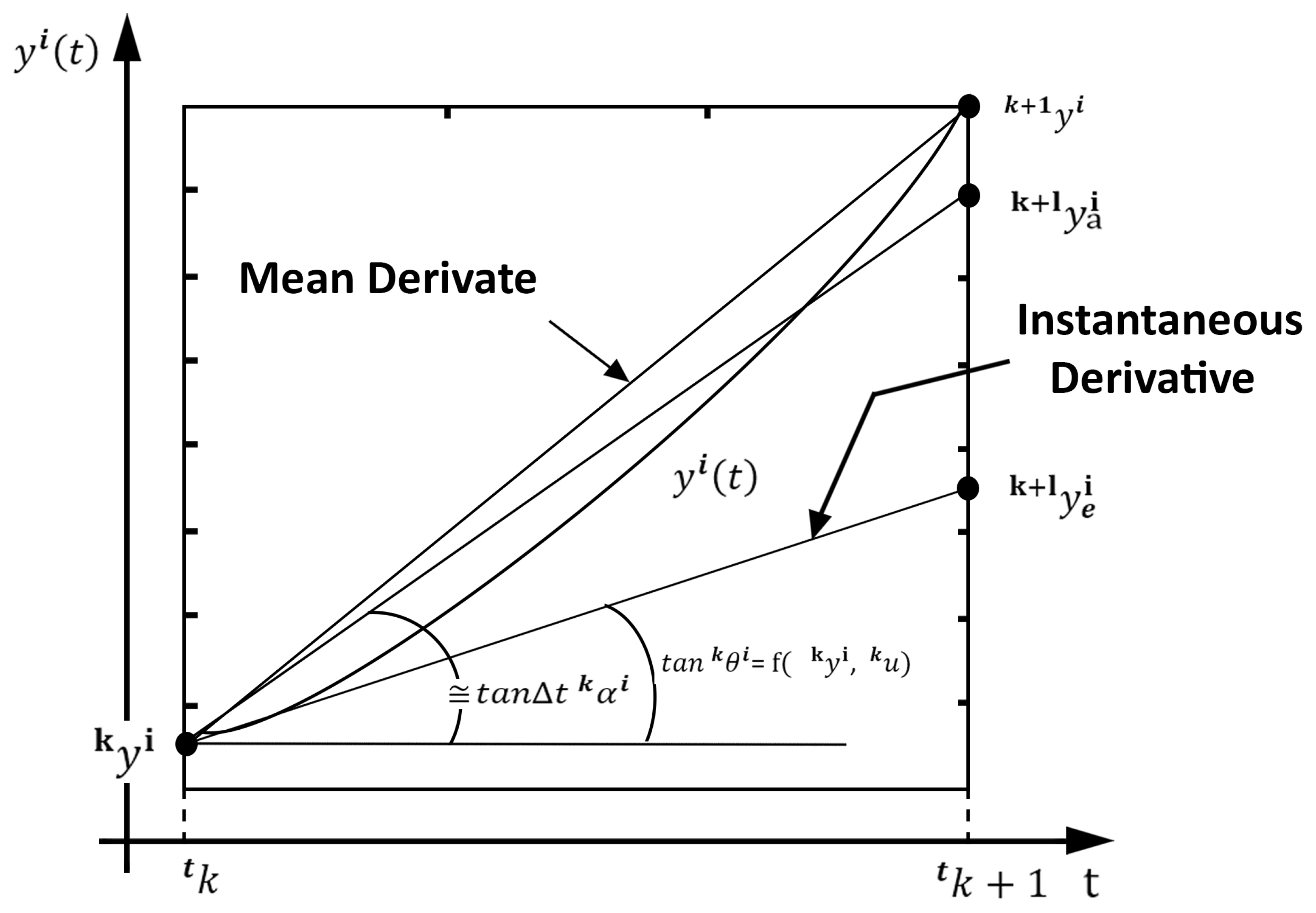
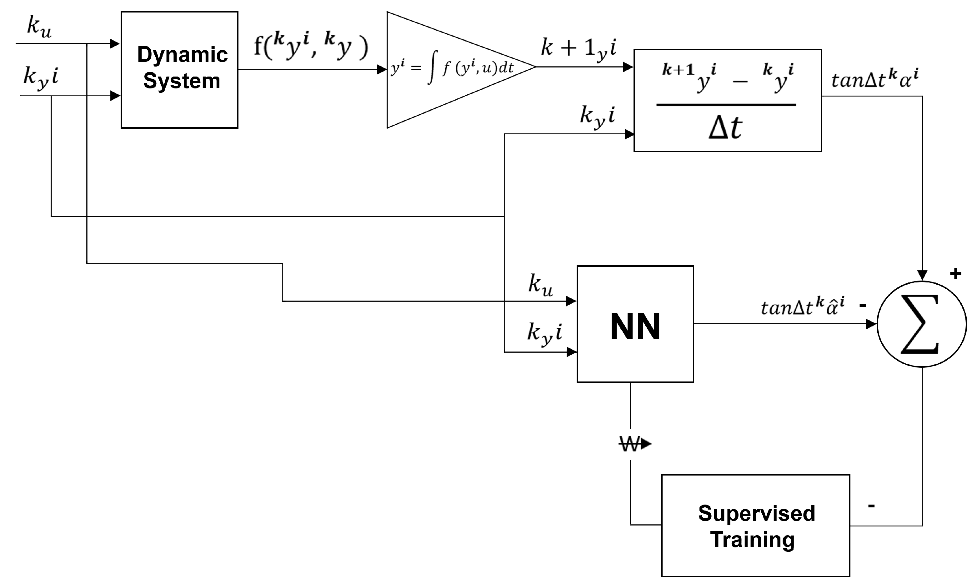
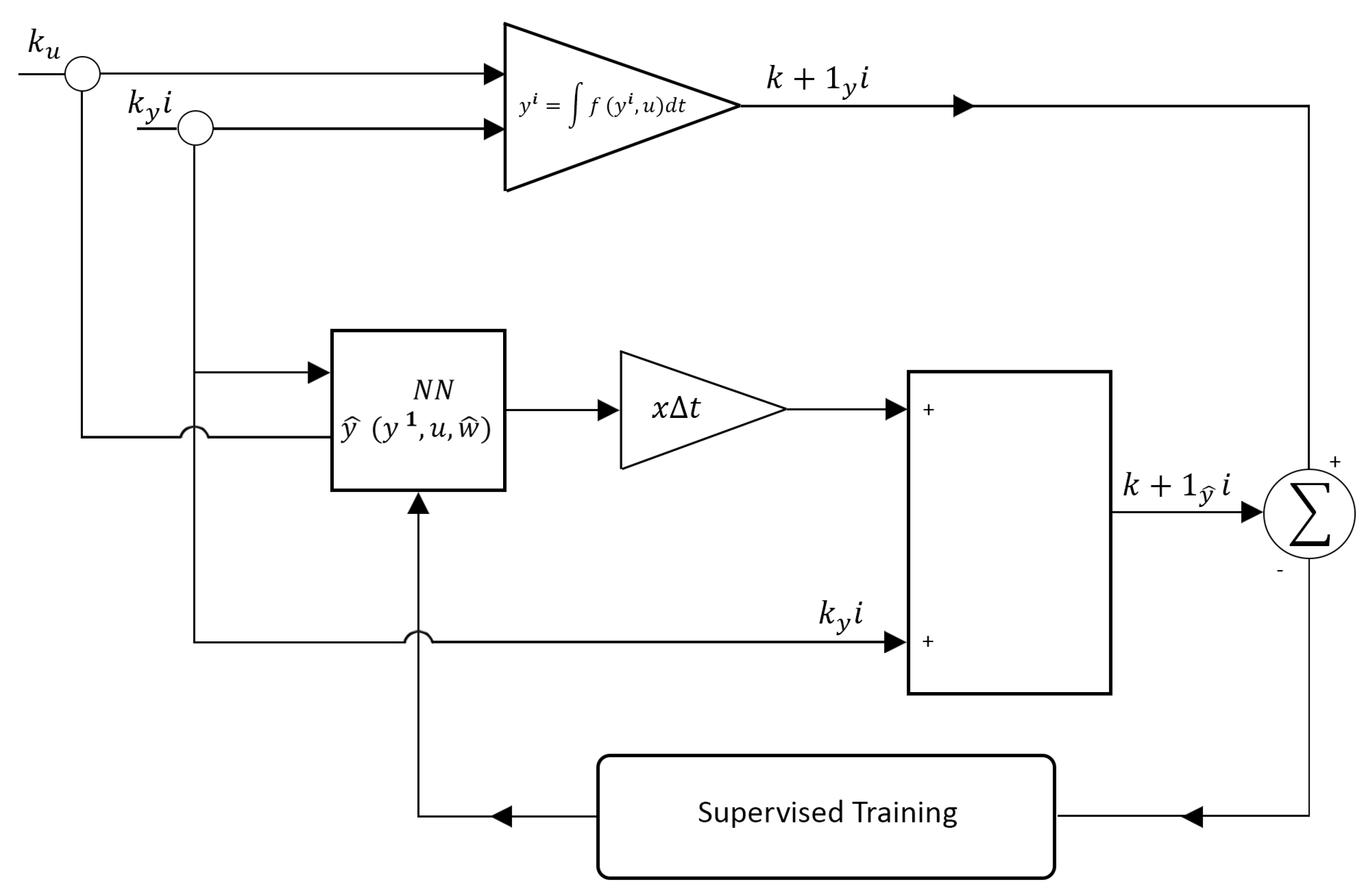
Figure 5.
A MLP neural network designed with the concept of mean derivative functions.
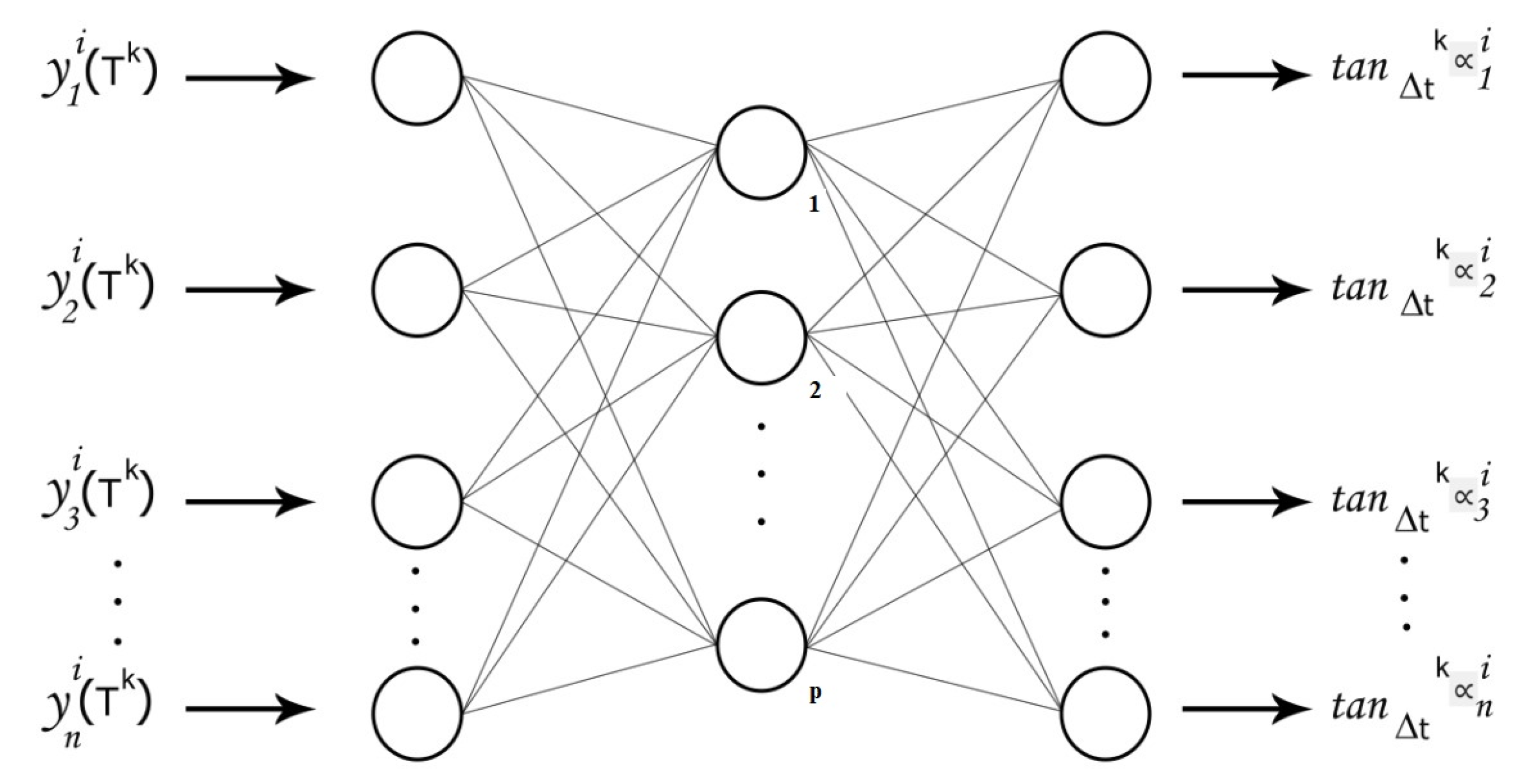
Figure 6.
Geometric finding that instantaneous derivative functions are symmetric, but mean derivative functions are not.
Figure 6.
Geometric finding that instantaneous derivative functions are symmetric, but mean derivative functions are not.
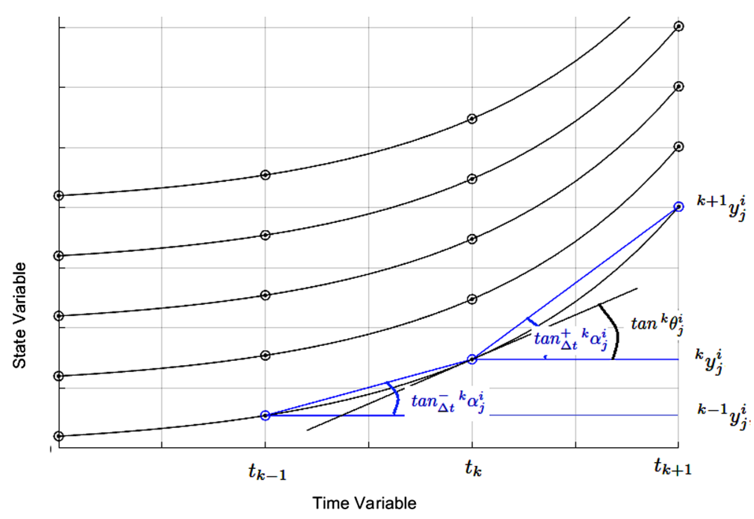
Figure 7.
The dynamics of example 1 solved with Runge-Kutta 4-5, available in Matlab with step automation through the "ode45.m" function, using forward and backward integrations.
Figure 7.
The dynamics of example 1 solved with Runge-Kutta 4-5, available in Matlab with step automation through the "ode45.m" function, using forward and backward integrations.
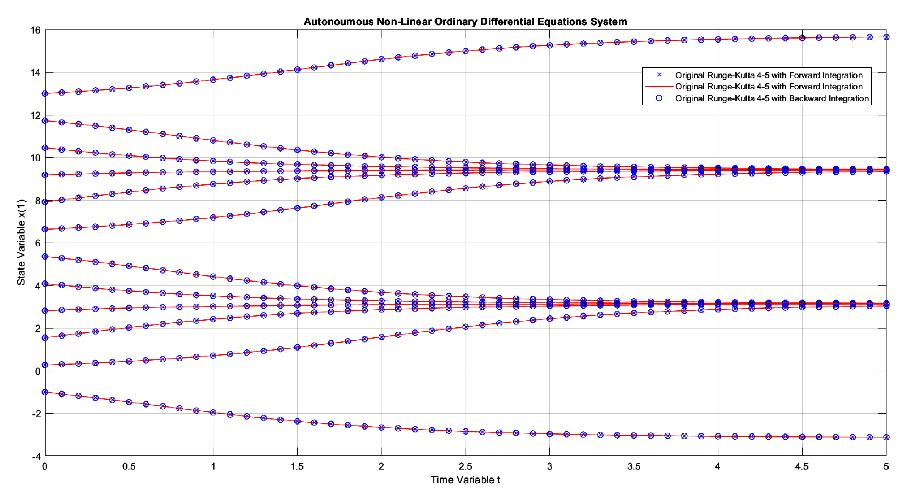
Figure 8.
The dynamics of example 1, comparing the conventional Euler integrator with E-TUNI, using forward and backward integrations with .
Figure 8.
The dynamics of example 1, comparing the conventional Euler integrator with E-TUNI, using forward and backward integrations with .
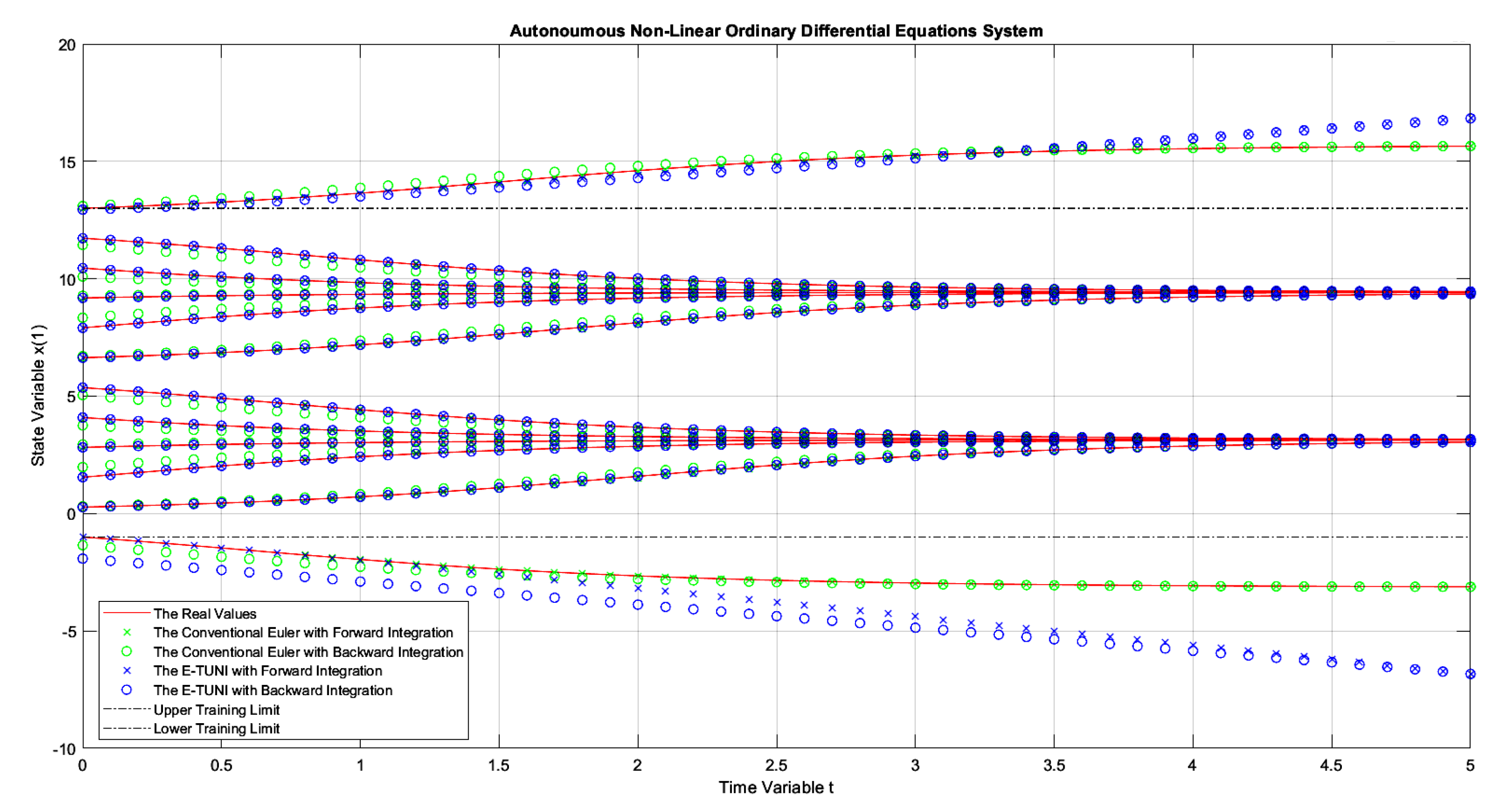
Figure 9.
The dynamics of example 1, comparing the conventional Euler integrator with E-TUNI, using forward and backward integrations with .
Figure 9.
The dynamics of example 1, comparing the conventional Euler integrator with E-TUNI, using forward and backward integrations with .
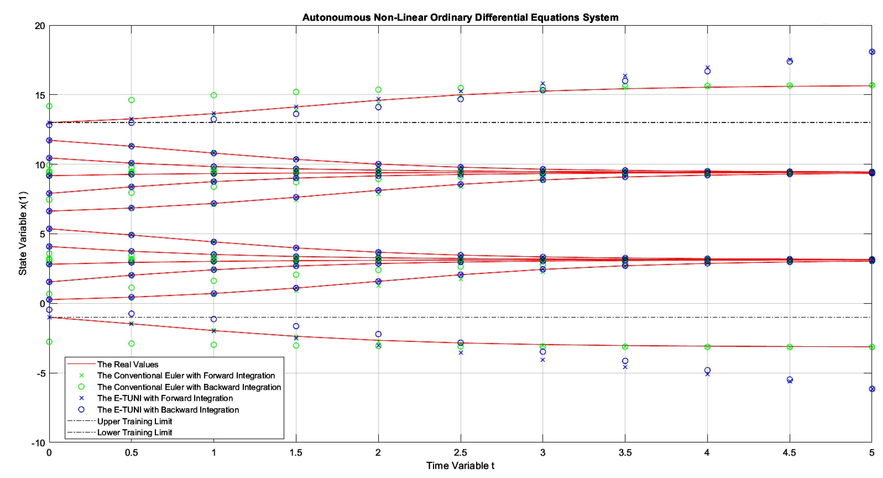
Figure 10.
The dynamics of example 1, comparing the conventional Euler integrator with E-TUNI, using forward and backward integrations with .
Figure 10.
The dynamics of example 1, comparing the conventional Euler integrator with E-TUNI, using forward and backward integrations with .
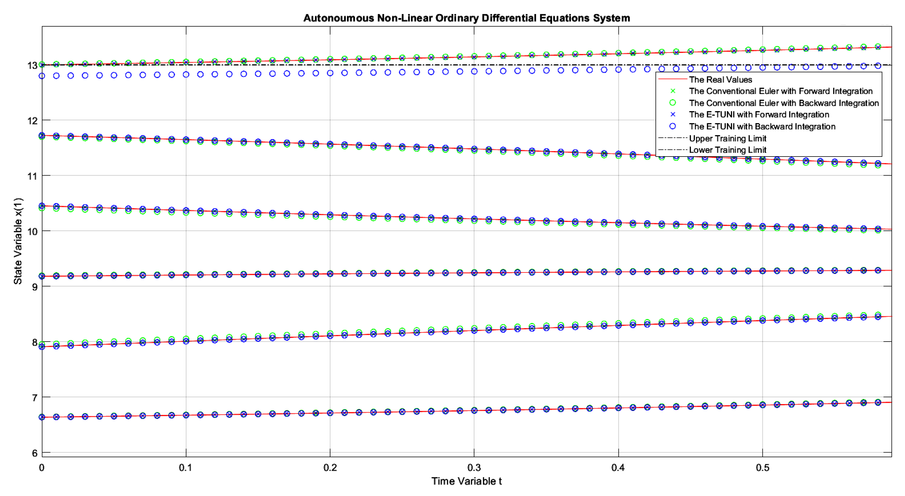
Figure 11.
The dynamics of example 1, comparing the conventional Euler integrator with E-TUNI, using forward and backward integrations with and being integrated up to .
Figure 11.
The dynamics of example 1, comparing the conventional Euler integrator with E-TUNI, using forward and backward integrations with and being integrated up to .
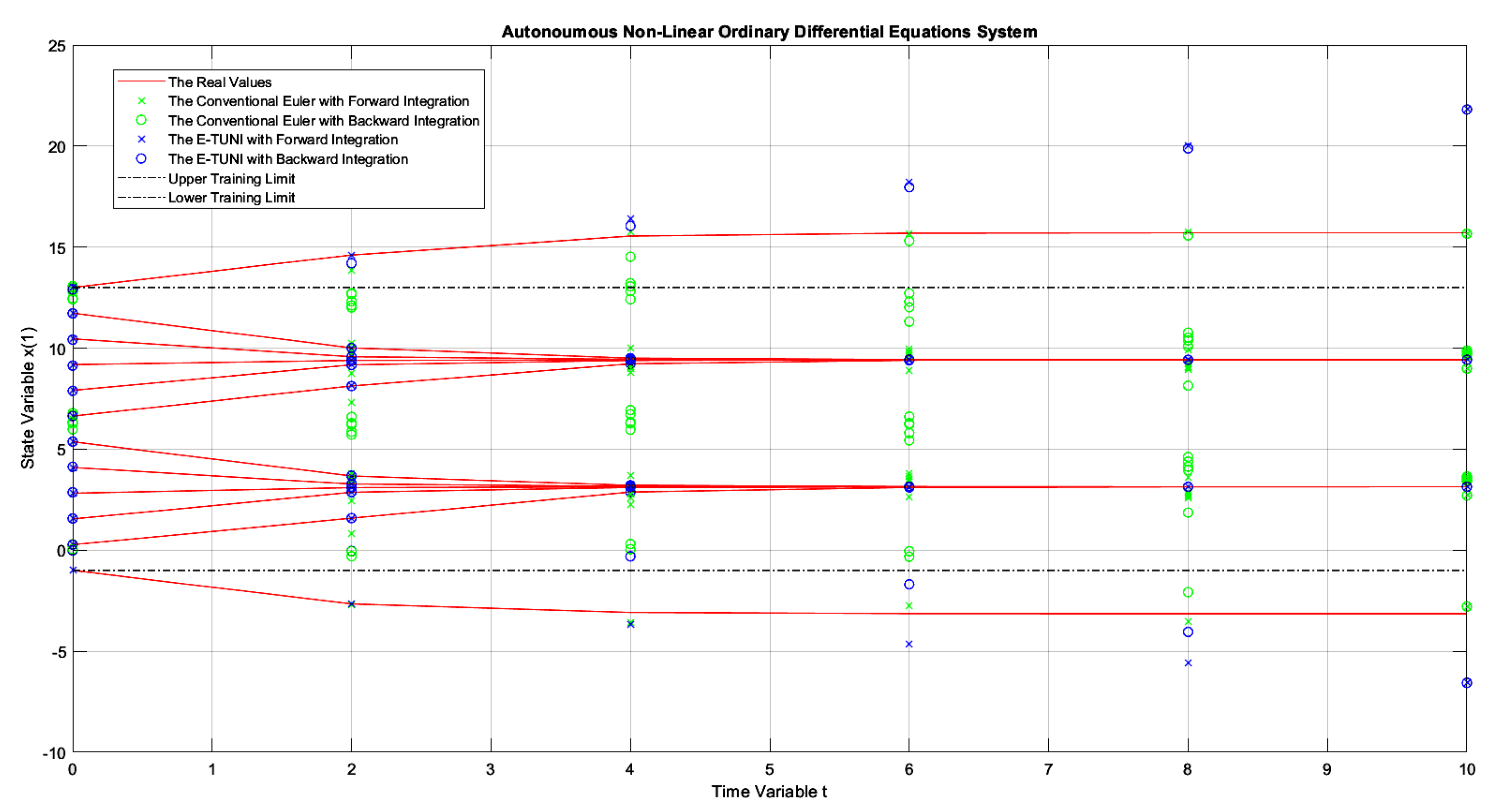
Figure 12.
The dynamics of example 1, comparing the conventional Euler integrator with E-TUNI, using forward and backward integrations with and being integrated up to .
Figure 12.
The dynamics of example 1, comparing the conventional Euler integrator with E-TUNI, using forward and backward integrations with and being integrated up to .
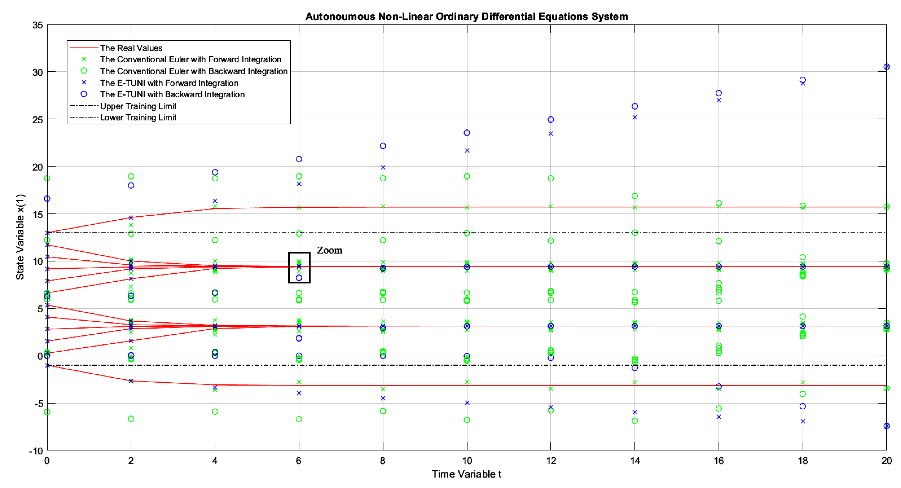
Figure 13.
The same example as in Figure 7, but instead of being integrated up to , it was integrated up to (notice the dissolution of the solution).
Figure 13.
The same example as in Figure 7, but instead of being integrated up to , it was integrated up to (notice the dissolution of the solution).

Figure 14.
The dynamics of example 2, comparing the conventional Euler integrator with E-TUNI, using forward and backward integrations with .
Figure 14.
The dynamics of example 2, comparing the conventional Euler integrator with E-TUNI, using forward and backward integrations with .
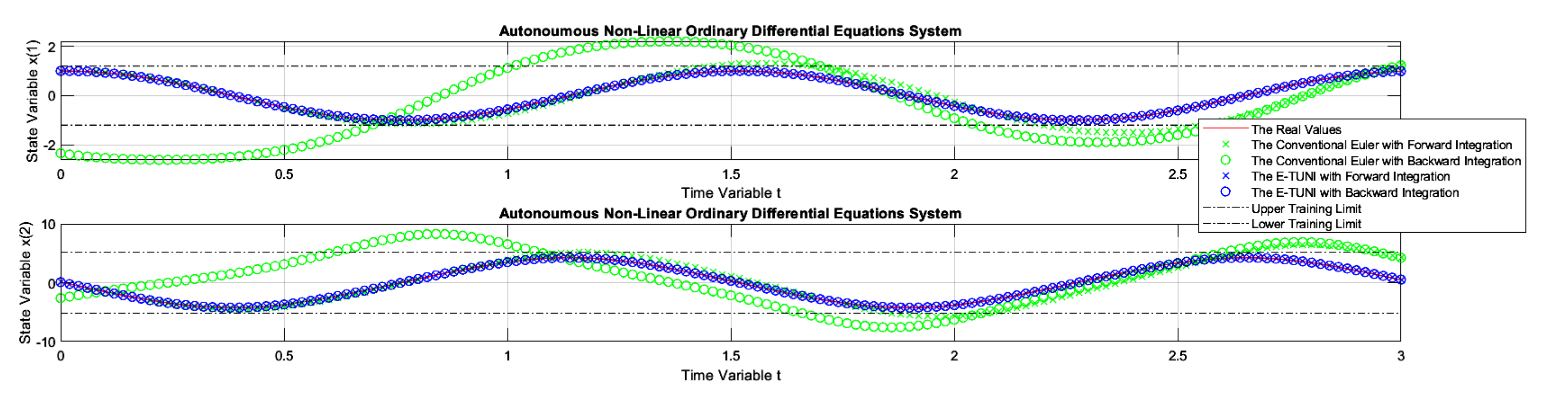
Figure 15.
The dynamics of example 2, comparing the conventional Euler integrator with E-TUNI, using forward and backward integrations with .
Figure 15.
The dynamics of example 2, comparing the conventional Euler integrator with E-TUNI, using forward and backward integrations with .
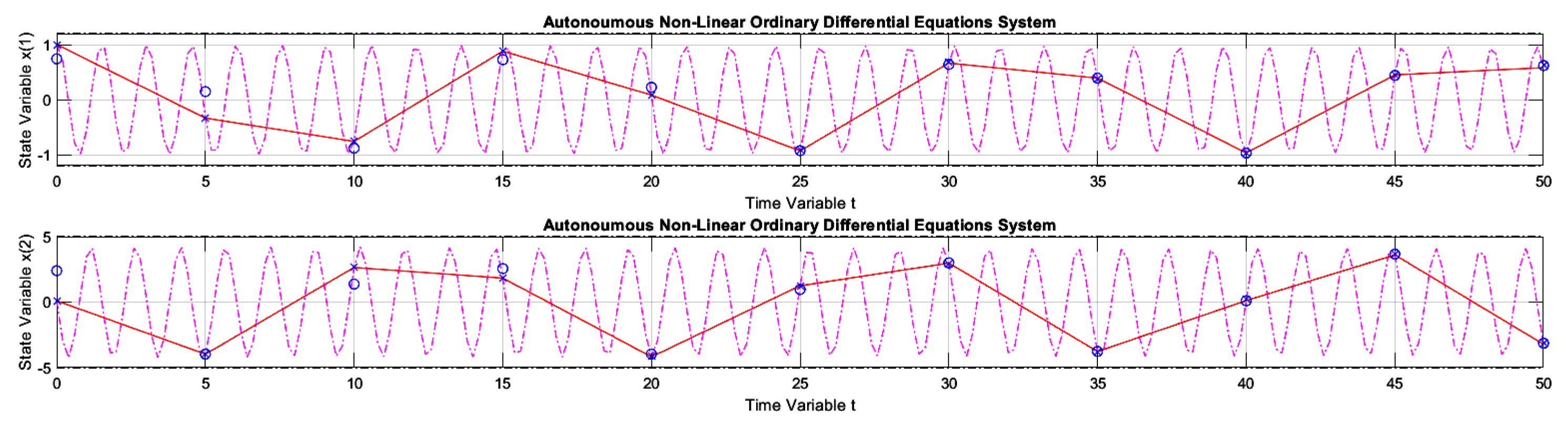
Figure 16.
The dynamics of example 2 solved with Runge-Kutta 4-5, available in Matlab with step automation through the "ode45.m" function, using forward and backward integrations.
Figure 16.
The dynamics of example 2 solved with Runge-Kutta 4-5, available in Matlab with step automation through the "ode45.m" function, using forward and backward integrations.

Figure 17.
The dynamics of example 3 solved with Runge-Kutta 4-5, available in Matlab with step automation through the "ode45.m" function, using forward and backward integrations.
Figure 17.
The dynamics of example 3 solved with Runge-Kutta 4-5, available in Matlab with step automation through the "ode45.m" function, using forward and backward integrations.
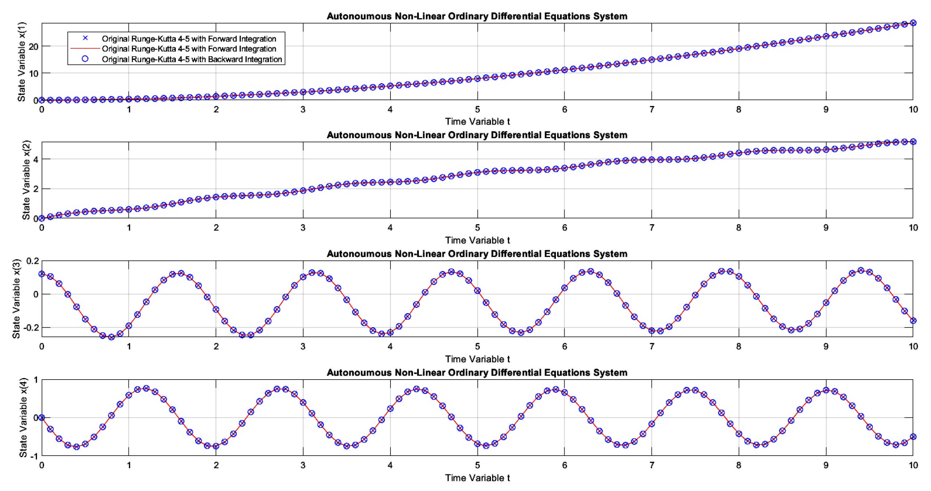
Figure 18.
The dynamics of example 3, comparing the conventional Euler integrator with E-TUNI, using forward and backward integrations with .
Figure 18.
The dynamics of example 3, comparing the conventional Euler integrator with E-TUNI, using forward and backward integrations with .
Disclaimer/Publisher’s Note: The statements, opinions and data contained in all publications are solely those of the individual author(s) and contributor(s) and not of MDPI and/or the editor(s). MDPI and/or the editor(s) disclaim responsibility for any injury to people or property resulting from any ideas, methods, instructions or products referred to in the content. |
© 2024 by the authors. Licensee MDPI, Basel, Switzerland. This article is an open access article distributed under the terms and conditions of the Creative Commons Attribution (CC BY) license (http://creativecommons.org/licenses/by/4.0/).
Copyright: This open access article is published under a Creative Commons CC BY 4.0 license, which permit the free download, distribution, and reuse, provided that the author and preprint are cited in any reuse.


