Submitted:
26 January 2023
Posted:
02 February 2023
You are already at the latest version
Abstract
The Van der Pol oscillator is a chaotic non-linear system. Small perturbations in initial conditions may result in wildly different trajectories. Because of its chaotic nature, controlling, or forcing, the behavior of a Van der Pol oscillator is difficult to achieve through traditional adaptive control methods. Connecting two Van der Pol oscillators together where the output of one oscillator, the driver, drives the behavior of its partner, the responder, is a proven technique for controlling the Van der Pol oscillator. Deterministic AI (DAI) is an adaptive feedback control method that leverages the known physics of the Van der Pol system to learn optimal system parameters for the forcing function. We assessed the performance of DAI employing three different online parameter estimation algorithms. Our evaluation criteria include mean absolute error (MAE) between the target trajectory and the response oscillator trajectory over time. RLS with exponential forgetting (RLS-EF) had the lowest MAE overall, with a 2.46% reduction in error. However, another method was notable. Least Mean Squares with normalized gradient adaptation (LMS-NG) had worse initial error in the first 10% of the simulation, but after that point had consistently better performance. We found that over the last 90% of the simulation, DAI with LMS-NG had a 48.7% reduction in MAE compared to feedforward alone.
Keywords:
chaotic systems
; Van der Pol oscillator
; drive-response
; synchronization of chaotic systems
; global chaos synchronization
; deterministic artificial intelligence
; feedforward
; feedback
; non-linear adaptive control
; online estimation
; recursive least squares (RLS)
; exponential forgetting
; Kalman filter
; least mean squares (LMS)
1. Introduction
The concept of chaos theory can be illustrated through the butterfly effect: the flapping of a butterfly’s wings can create a small gust of air that ultimately leads to a storm on the other side of the world. Chaos theory refers to systems that are bounded, recurrent, and highly sensitive to initial conditions (see Figure 1). For example, weather patterns are chaotic systems that can be influenced by small changes in initial conditions such as temperature, pressure, and wind patterns. This sensitivity to initial conditions makes predicting the weather challenging, even with the help of advanced computers.
In 2000, Boccalettia reviewed the major ideas involved in the control of chaos and proposed two methods: the Ott–Grebogi–Yorke (OGY) method and the adaptive method both seeking to bring a trajectory to a small neighborhood of a desired location, seeking stabilized desired chaotic orbits embedded in a chaotic attractor including a review of relevant experimental applications of the techniques [2]. Ott, C. Grebogi and J. A. Yorke observed that the infinite number of unstable periodic orbits typically embedded in a chaotic attractor could be taken advantage of for the purpose of achieving control by means of applying only very small perturbations [3]. Song, et. al, proposed combining feedback control with OGY method [4], and this trend to utilize feedforward followed by application of feedback might be considered canonical. Back in 1992, Pyragas had already offered continuous control of chaos by self-controlling feedback [4].
Adaptive methods as offered by Slotine and Li [5] strictly rely on a feedforward implementation augmented by feedback adaption of the feedforward dynamics, but also utilize elements of classical feedback adaption (e.g. the M.I.T. rule [6]) to adapt classical feedback control gains and adapt the desired trajectory to eliminate tracking errors. Following kinetic improvements to Slotine’s approach by Fossen [7,8] and subsequent researchers [9] the approach was experimentally validated in [10]. In 2017, Cooper and Heidlaulf [11] proposed extracting the feedforward elements of Slotine’s approach for controlling chaos of the famous van der Pol oscillator [12] which has grown to become a benchmark system for representing chaotic systems like relaxation oscillators [13], frequency demultiplication [14], heartbeats [15] and nonlinear electric oscillators in general [16].
Cooper and Heidlauf’s techniques were initially paired with linear feedback control (linear quadratic optimal control), but the combination of feedback and feedforward proved ineffective. Smeresky and Rizzo offered 2-norm optimal feedback using pseudoinverse in 2020 [17], and the combination proved effective for controlling highly nonlinear, coupled (non-chaotic) Euler’s moment equations. The combination of feedforward and optimal feedback learning was formulated for five-degree of freedom oceanic vehicles in [18] and labeled deterministic artificial intelligence. Shortly afterwards, Zhai directly compared stochastic artificial intelligence methods: neural networks and physics-informed deep learning in [19,20].
Originally discovered by Gauss in the 1800s, the work lay unused until Plackett rediscovered his work and applied it to signal processing [21]. Several methods have emerged since extending and resolving weakness of the recursive least squares method. Several of these such as the addition of exponential forgetting and posterior residuals their follow-on techniques are discussed by Astrom and Wittenmark and in their textbook on adaptive control [22]. However, these works often fail to consider the cost required to determine the control input dependence of the system. In order to excite the system so that the response can be observed, and a model fit to it, resources such as fuel or electric power must be expended. In addition, the convergence rate per unit cost may be deciding factor when choosing an approach. A controller must understand the system it is controlling before it is able to drive it to a desired state. A secondary challenge is the inherent non-linearity of many systems present in real world applications. Such systems cannot be written using simple linear models with respect to the system states and require different analysis techniques. An overview of existing analysis methods can be found in [23]. However, as mentioned before these techniques do not attempt to minimize the cost of system identification. It is demonstrated in this work that an excitation controller based on optimal learning techniques and self-awareness statements provides a significantly higher accuracy per unit cost than other excitation signals. Optimal learning and self-awareness are components of deterministic artificial intelligence, which seeks to create intelligent systems that derive results through conditions restricted to obey physical models rather than purely stochastically through bulk data.
In this manuscript, we focus on the Van der Pol chaotic oscillator. Scientists have used this chaotic system for multiple applications, such as modeling action potentials and countering electromagnetic pulse attacks. Adaptive control theory offers a means of stabilizing the Van der Pol system through synchronization of a drive and response system.
Cooper and Heidlauf showed that the Van der Pol system can be forced to asymptotically follow a desired trajectory in [11]. They accomplished this by using a Van der Pol oscillator, the driver, to force another Van der Pol oscillator, the responder. We refer to this technique as feedforward Van der Pol.
Smeresky and Rizzo proposed an improvement on feedforward Van der Pol in [17] using deterministic artificial intelligence (DAI). The DAI method combines nonlinear adaptive control and physics-based controls methods. It is based on self-awareness statements enhanced by optimal feedback, which is reparametrized into a standard regression form. Online estimation methods such as recursive least squares estimate the system parameters for this optimal feedback.
This manuscript compares the performance of DAI for non-linear adaptive control of a Van der Pol oscillator when using three different online estimation methods: a Kalman filter, recursive least squares with exponential forgetting (RLS-EF), and least mean squares with a normalized gradient (LMS-NG).
2. Materials and Methods
The Van der Pol chaotic oscillator is defined by Equation (1):
where , , and define the system parameters, , and is the forcing function. With DAI, the system parameters are estimated at each time step. Figure 3 is a Simulink model that represents the system.
, drives the Van der Pol oscillator. State information is passed into the forcing function block, to be used by DAI to estimate the system parameters.
Online estimation methods analyzed in this paper require two inputs: the regressors observed from the system and from the previous time step, . We define the regressors as:
Given system inputs and , the estimator performs regression to calculate the estimated system parameters, . These are used in conjunction with self-awareness statements to calculate .
Self-awareness statements are formulated using desired trajectory :
and represent the known physics of the Van der Pol system. All together, we have Equation (4):
3. Results
We used the Runge-Kutta MATLAB 2022b solver in Simulink with a step size of 0.01 and a simulation time of 100 seconds to run the model in Figure 3 given different forcing functions:
- Unforced
- Uniform noise
- Sine wave
- Feedforward
- Deterministic artificial intelligence (DAI) – Kalman estimator
- Deterministic artificial intelligence (DAI) – RLS-EF estimator
- Deterministic artificial intelligence (DAI) – LMS-NG estimator
For the deterministic artificial intelligence methods, we initialized (, , and ) as 0.1; the ground truth value was . Despite the inaccuracy of the initial estimates, all deterministic artificial intelligence methods succeeded in iteratively estimating the truth values, with converging to .

Table 1.
Mean absolute error (MAE) for the entire trajectory.
| Method | Method | ||
|---|---|---|---|
| 1 | 3.3234 | 1 | 3.2031 |
| 2 | 3.3334 | 2 | 3.2110 |
| 3 | 3.9843 | 3 | 3.9275 |
| 4 | 0.2091 | 4 | 0.2284 |
| 5 | 0.4975 | 5 | 0.3927 |
| 6 | 0.2041 | 6 | 0.2237 |
| 7 | 0.3089 | 7 | 0.2877 |
Table 2.
Mean absolute error (MAE) when excluding the first 10% of the trajectory.
| Method | Method | ||
|---|---|---|---|
| 1 | 3.3218 | 1 | 3.1891 |
| 2 | 3.3262 | 2 | 3.1941 |
| 3 | 4.0150 | 3 | 3.9487 |
| 4 | 0.0642 | 4 | 0.0743 |
| 5 | 0.1220 | 5 | 0.1379 |
| 6 | 0.0629 | 6 | 0.0728 |
| 7 | 0.0329 | 7 | 0.0599 |
We analyzed the error between the trajectory of the responder Van der Pol oscillator and the desired trajectory, a circle of radius 5. The first three methods did not employ feedforward or deterministic artificial intelligence feedback. The unforced and uniform noise forced oscillators both exhibited the expected chaotic trajectory of a Van der Pol oscillator, visualized at the center of Figure 6. The sine wave forced the responder oscillator to deviate from the typical Van der Pol trajectory, but the resulting trajectory was chaotic.
The method 4, feedforward using the drive-response methodology in [1], successfully forced the responder oscillator to follow the target trajectory. Methods 5-7 built upon method 4, adding deterministic artificial intelligence feedback as described in [25] to estimate and learn the system parameters.
4. Discussion
A Van der Pol oscillator subtends toward a limit cycle, an invariant set determined by the initial conditions. This occurs when both sides of Equation (1) are equal; or:
In other words, the oscillator will, after some time, converge to a fixed trajectory. The goal of [1] was to command a Van der Pol oscillator such that, no matter the initial conditions, it will asymptotically approach the same limit cycle. Smeresky and Rizzo went a step further in [25] by showing that deterministic artificial intelligence (DAI) can improve the ability of the forcing function, , to force the responder oscillator to follow a desired trajectory.
We build upon the results of [25] by comparing three different DAI system parameter estimators: a Kalman filter, recursive least squares with exponential forgetting (RLS-EF), and least mean squares with a normalized gradient (LMS-NG).
For all methods with feedforward (methods 4-7), the responder Van der Pol oscillator has significant error in the beginning that decreases as the oscillator stabilizes to the desired trajectory. This error approaches zero.
Over the length of the entire simulation, 10,000 time steps for 100 seconds at a sample time of 0.01, the DAI estimator that had the lowest mean absolute error (MAE) was RLS-EF, with a 2.41% and 2.01% reduction in MAE for and , respectively, compared to feedforward alone. See the first two results columns of Table 3 for percent improvement. We found that DAI with the Kalman filter and LMS-NG had worse performance than feedforward alone. These results suggested that the Kalman filter and LMS-NG estimators should be avoided in favor of RLS-EF.
However, we noticed that DAI using the LMS-NG estimator exhibited decreased MAE as the system approached the limit cycle. See the last two results columns of Table 3 for percent improvement after t=1000. DAI with LMS-NG had 48.7% and 19.3% less MAE for and , respectively, compared to feedforward alone, and exhibited a 47.7% and 17.7% reduction in MAE for and compared to DAI with RLS-EF.
Our results show that the RLS-EF algorithm for parameter estimation is optimal for the first 1,000 time steps of the simulation, after which LMS-NG exhibits superior performance. One algorithm may be preferable over the other depending on the intended application. For instance, RLS-EF having relatively minimal error when the system is far from the limit cycle could indicate that the algorithm is better-suited for systems where frequent external disturbances are expected.
As a next step for future research, both techniques could be used together, with the algorithm using RLS-EF for the first t time steps to estimate system parameters and then switching over to LMS-NG once the system has found stability. Another research opportunity would be adding logic for the model to switch between different estimation methods when an external disturbance to the system is introduced. Such efforts may build off the research of Sands [26] for countering the effects of electromagnetic pulses.
Appendix A
Matlab Code:
%%
clear all; close all; clc;
headless = 1;
RngSeed = 1;
% Oscillator Parameters
alpha=5;
mu=1;
beta=1;
% RLS Parameters
rls_sample_time=.01;
alpha_i = 0.1;
mu_i = 0.1;
beta_i = 0.1;
% Desired Trajectory Parameters
A=5;
omega=1;
SampleTime = .01;
% Initial Conditions
x0 = 1;
v0 = 1;
%%
figure(1);
hold on;
errors = [];
errors2 = [];
episodes = 6001;
forgetting_factor = 1;
noise_covariance = 80;
adaption_gain = .9277;
grab_index = 1000;
for Index=1:1:3
sim('SimVanDerPol');
errors = [errors; mean(abs(states - desiredstates(1:2,:)'))]
errors2 = [errors2; mean(abs(states(grab_index:end,:) - desiredstates(1:2,grab_index:end)'))]
figure(1);
plot(states(:,1), states(:,2),':', 'Linewidth',2);hold on;
end
for Index=4:1:7
sim('SimVanDerPol');
errors = [errors; mean(abs(states - desiredstates(1:2,:)'))]
errors2 = [errors2; mean(abs(states(grab_index:end,:) - desiredstates(1:2,grab_index:end)'))]
figure(1);
plot(states(:,1), states(:,2),':', 'Linewidth',2);hold on;
figure(2);
subplot(1,4,Index-3);plot(states(grab_index:end,1) - desiredstates(1,grab_index:end)');axis([0,length(desiredstates(1,grab_index:end)),-0.025,0.025]);
end
figure(1);
plot(desiredstates(1,:), desiredstates(2,:),':', 'Linewidth',1, 'Color', 'red');hold off;
legend("Unforced", "Random Noise", "Sine Wave", "Feedforward", "RLS Kalman", "RLS-EF", "Norm'd LMS", "Goal",'fontname','Palatino', 'fontsize',22,'NumColumns',2,'Location','northeast','Orientation','horizontal');
set(gca,'fontname','Palatino', 'fontsize',26);
axis([-9,9,-9,9]);
xlabel("x(t)",'fontname','Palatino', 'fontsize',32); ylabel("dx(t)/dt",'fontname','Palatino', 'fontsize',26);
figure(3);
subplot(1,2,1);plot(abs(errors(:,1)));
subplot(1,2,2);plot(abs(errors(:,2)));
References
- Rubinsztejn, Ari. Three double pendulums with near identical initial conditions diverge over time displaying the chaotic nature of the system. 2018. Available online: https://upload.wikimedia.org/wikipedia/commons/thumb/e/e3/Demonstrating_Chaos_with_a_Double_Pendulum.gif/330px-Demonstrating_Chaos_with_a_Double_Pendulum.gif. (accessed on 22 12 2022).
- Cassady, J.; Maliga, K.; Overton, S.; Martin, T.; Sanders, S.; Joyner, C.; Kokam, T.; Tantardini, M. Next Steps in the Evolvable Path to Mars. In Proceedings of the International Astronautical Congress, Jerusalem, Israel, 12-16 October 2015. [Google Scholar]
- Song, Y.; Li, Y. Li, C. Ott-Grebogi-Yorke controller design based on feedback control. 2011 International Conference on Electrical and Control Engineering, Yichang, China, 24 October 2011, pp. 4846-4849.
- Pyragas, K. Continuous control of chaos by self-controlling feedback. Physics Letters A 1992, 170(6), 421–428. [Google Scholar] [CrossRef]
- Slotine, J.; Li, W. Applied Nonlinear Control; Prentice-Hall, Inc.: Englewood Cliffs, NJ, U.S.A, 1991; pp. 392–436. [Google Scholar] [CrossRef]
- Osburn, J.; Whitaker, H.; Kezer, A. New developments in the design of model reference adaptive control systems. Inst. Aero. Sci. 196161(39).
- Fossen, T. Handbook of Marine Craft Hydrodynamics and Motion Control, 2 ed.; John Wiley & Sons Inc.: Hoboken, USA, 2021. [Google Scholar]
- Fossen, T. Guidance and Control of Ocean Vehicles; John Wiley & Sons Inc.: Chichester, UK, 1994. [Google Scholar]
- Sands, T.; Kim, J.; Agrawal, B. Spacecraft fine tracking pointing using adaptive control. Proceedings of 58th International Astronautical Congress, International Astronautical Federation: Paris, France, 24-28 September 2007.
- Sands, T.; Kim, J.; Agrawal, B. Spacecraft Adaptive Control Evaluation. Infotech@Aerospace, Garden Grove, California, 19 - 21 June 2012.
- Cooper, M.; Heidlauf, P.; Sands, T. Controlling Chaos—Forced van der Pol Equation. Mathematics 2017, 5, 70. [Google Scholar] [CrossRef]
- van der Pol, B. A note on the relation of the audibility factor of a shunted telephone to the antenna circuit as used in the reception of wireless signals, Philosophical Magazine 1917, 34, 184–8. [CrossRef]
- van der Pol, B. On “Relaxation Oscillations”. I. Philos. Mag. 1926, 2, 978–992. [Google Scholar] [CrossRef]
- van der Pol, B.; van der Mark, J. Frequency Demultiplication. Nature 1927, 120, 363–364. [Google Scholar] [CrossRef]
- van der Pol, B.; van der Mark, J. The heartbeat considered as a relaxation-oscillation, and an electrical model of the heart. Philosophical Magazine 1929, 6, 673–75. [Google Scholar] [CrossRef]
- van der Pol, B. The nonlinear theory of electric oscillations. Proc. IRE 1934, 22, 1051–1086. [Google Scholar] [CrossRef]
- Smeresky, B.; Rizzo, A.; Sands, T. Optimal Learning and Self-Awareness Versus PDI. Algorithms 2020, 13, 23. [Google Scholar] [CrossRef]
- Sands, T. Development of Deterministic Artificial Intelligence for Unmanned Underwater Vehicles (UUV). J. Mar. Sci. Eng. 2020, 8, 578. [Google Scholar] [CrossRef]
- Zhai, H.; Sands, T. Controlling Chaos in Van Der Pol Dynamics Using Signal-Encoded Deep Learning. Mathematics 2022, 10, 453. [Google Scholar] [CrossRef]
- Zhai, H.; Sands, T. Comparison of Deep Learning and Deterministic Algorithms for Control Modeling. Sensors 2022, 22, 6362. [Google Scholar] [CrossRef] [PubMed]
- Plackett, R. ; Some Theorems in Least Squares. Biometrika 1950, 37, 149–157. [Google Scholar] [CrossRef] [PubMed]
- Astrom K., Wittenmark B. Adaptive Control. 2nd ed. Addison Wesley Longman: Massachusetts, USA; 1995.
- Patra, A.; Unbehauen, H. Nonlinear modeling and identification. In IEEE/SMC’93 Conference System Engineering in Service of Humans, Le Touquet, France, October 17-20, 1993.
Figure 1.
The double pendulum simulation. A double pendulum is a chaotic system. Infinitesimal changes in initial conditions cause divergence in motion [1].
Figure 1.
The double pendulum simulation. A double pendulum is a chaotic system. Infinitesimal changes in initial conditions cause divergence in motion [1].
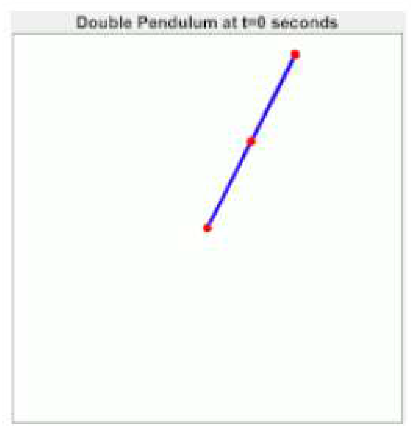
Figure 2.
The Van der Pol response oscillator is forced to follow a prescribed circular trajectory. Error between the response oscillator trajectory and the target trajectory asymptotically approaches zero.
Figure 2.
The Van der Pol response oscillator is forced to follow a prescribed circular trajectory. Error between the response oscillator trajectory and the target trajectory asymptotically approaches zero.
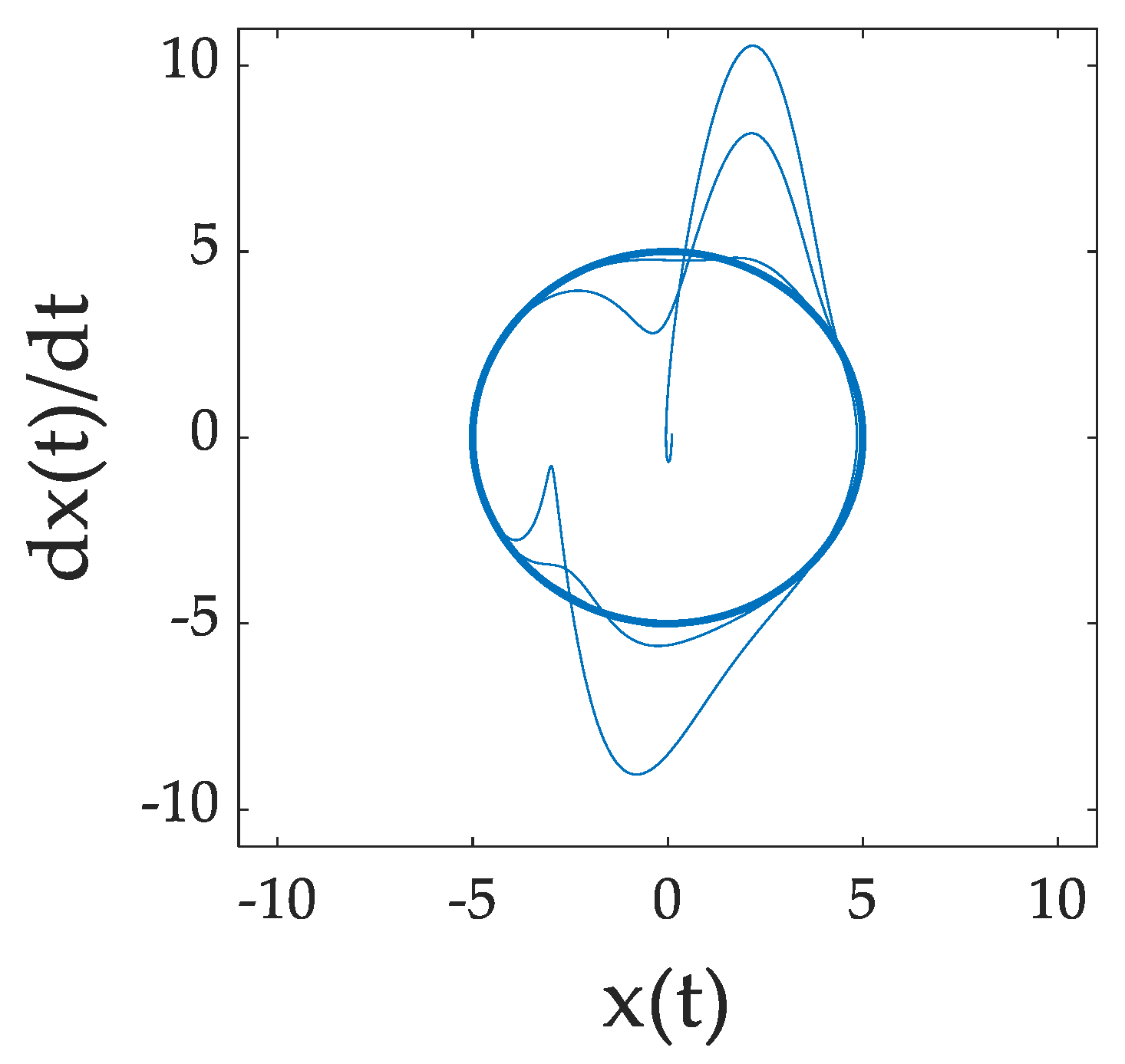
Figure 3.
The forcing function block,
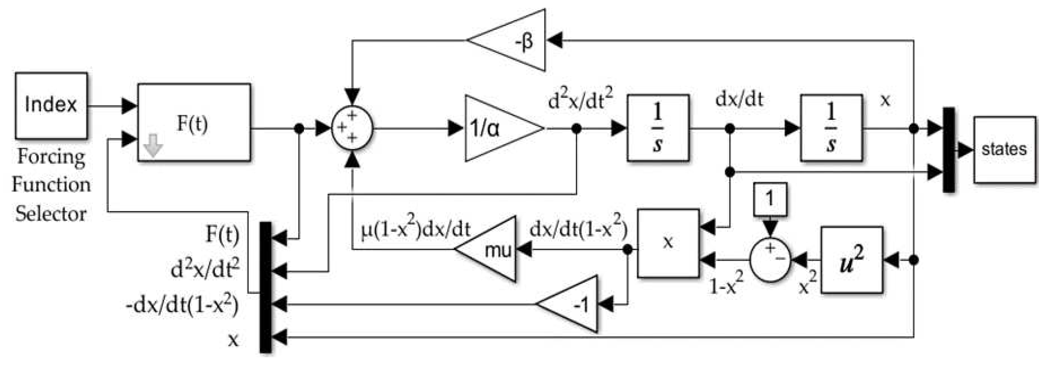
Figure 4.
The forcing function block, , with feedforward only.
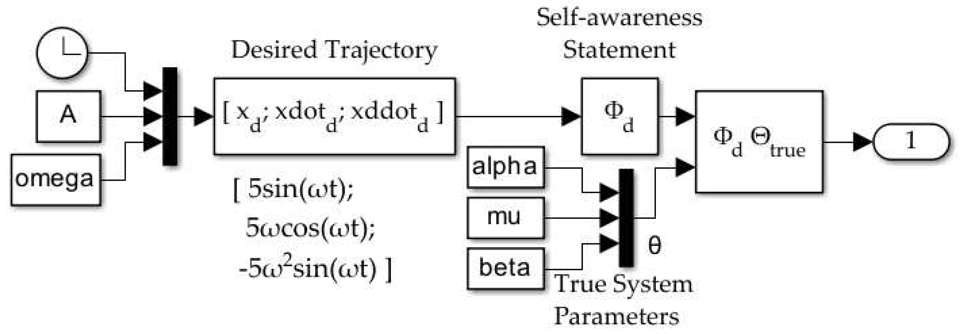
Figure 5.
The forcing function block, , adding DAI feedback as derived in [3]. In this paper, the Estimator block utilizes one of three methods to calculate : Kalman filter, RLS-EF, and LMS-NG.
Figure 5.
The forcing function block, , adding DAI feedback as derived in [3]. In this paper, the Estimator block utilizes one of three methods to calculate : Kalman filter, RLS-EF, and LMS-NG.
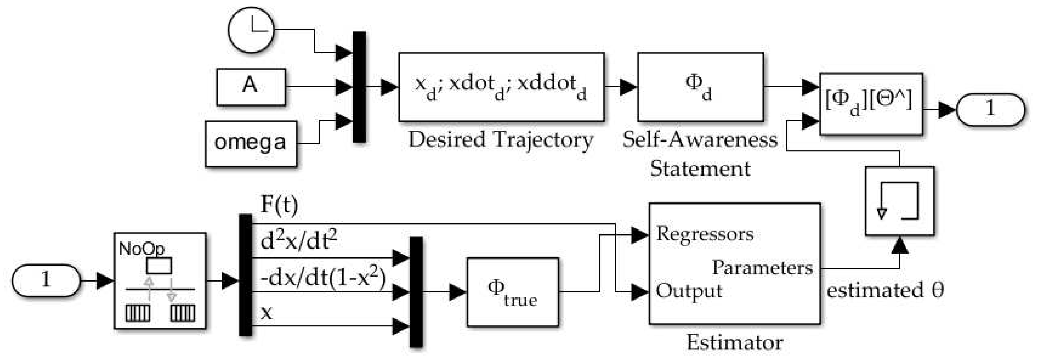
Figure 6.
The Van der Pol response oscillator trajectory plotted against the target (goal) trajectory, a circle of radius 5, for each of the forcing functions. Methods 4-7 successfully force the response oscillator to follow the target trajectory.
Figure 6.
The Van der Pol response oscillator trajectory plotted against the target (goal) trajectory, a circle of radius 5, for each of the forcing functions. Methods 4-7 successfully force the response oscillator to follow the target trajectory.
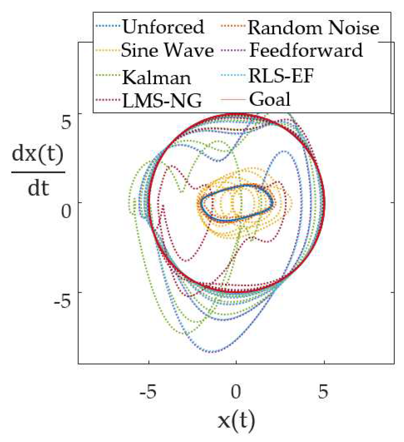
Figure 7.
Error of calculated over time for methods 4-7, in order. Note that the error curve of method 7, LMS-NG, is distinct from the others. MAE is used in assessing model performance to handle both positive and negative error swings.
Figure 7.
Error of calculated over time for methods 4-7, in order. Note that the error curve of method 7, LMS-NG, is distinct from the others. MAE is used in assessing model performance to handle both positive and negative error swings.
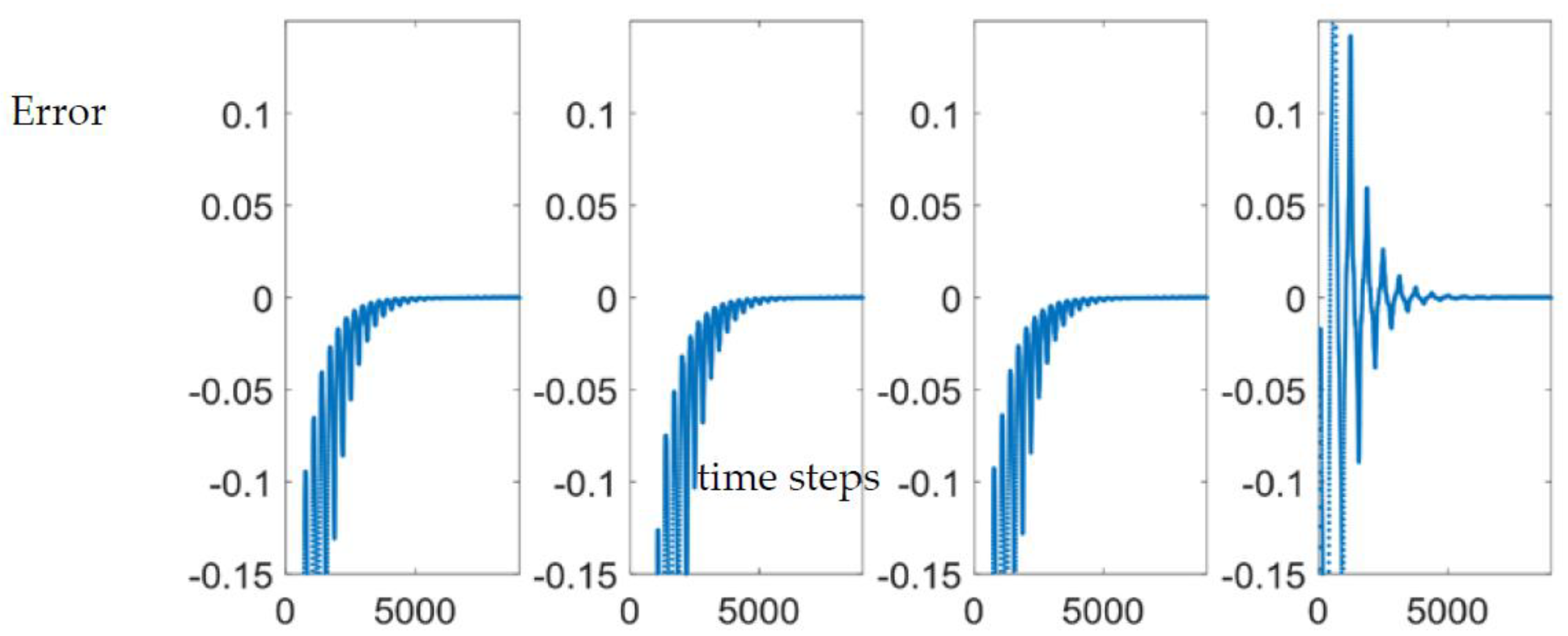
Table 3.
Performance comparison. Percent MAE improvement calculated between the DAI methods and method 4, feedforward only. Negative values indicate worse performance and are colored red. The best result in each column is bolded.
Table 3.
Performance comparison. Percent MAE improvement calculated between the DAI methods and method 4, feedforward only. Negative values indicate worse performance and are colored red. The best result in each column is bolded.
| Method |
(% ± rel. method 4) |
(% ± rel. method 4) |
(% ± rel. method 4) |
(% ± rel. method 4) |
|---|---|---|---|---|
| Feedforward Only (Method 4) | – | – | – | – |
| DAI with Kalman (Method 5) | -137.86 | -71.93 | -90.1 | -85.7 |
| DAI with RLS-EF (Method 6) | 2.41 | 2.04 | 1.97 | 1.93 |
| DAI with LMS-NG (Method 7) | -47.69 | -25.98 | 48.70 | 19.32 |
Disclaimer/Publisher’s Note: The statements, opinions and data contained in all publications are solely those of the individual author(s) and contributor(s) and not of MDPI and/or the editor(s). MDPI and/or the editor(s) disclaim responsibility for any injury to people or property resulting from any ideas, methods, instructions or products referred to in the content. |
© 2023 by the authors. Licensee MDPI, Basel, Switzerland. This article is an open access article distributed under the terms and conditions of the Creative Commons Attribution (CC BY) license (http://creativecommons.org/licenses/by/4.0/).
Copyright: This open access article is published under a Creative Commons CC BY 4.0 license, which permit the free download, distribution, and reuse, provided that the author and preprint are cited in any reuse.


