
Submitted:
31 October 2025
Posted:
03 November 2025
You are already at the latest version
Abstract
Safe and sample-conscious controller synthesis for nonlinear dynamics benefits from reinforcement learning that exploits a model of the plant. A nonlinear mass–spring–damper with hardening effects and hard stops is considered. Two data-driven models are employed to enable off-plant training: a piecewise linear model assembled from operating-region linear descriptions and blended by triangular memberships, and a global nonlinear autoregressive model with exogenous input constructed from past inputs and outputs. Q-learning is performed with the model in the loop using an error-indexed discrete state space, a finite force alphabet, and a reward that balances absolute tracking error with its short-horizon decrease. When the trained agents are deployed on the true plant for reference tracking, the piecewise linear model tends to yield tighter regulation near the setpoint and reduced steady-state bias, while the nonlinear autoregressive route requires less prior structural knowledge and a simpler data-collection campaign, at the cost of larger residual error in the tested scenario. These findings indicate that model-based Q-learning with data-driven models enables off-plant policy learning while containing experimental risk. Observed performance reflects a trade-off between fidelity obtained from localized linearization and generality afforded by global nonlinear regression, as well as design choices in state discretization and reward shaping. Prospective improvements include adaptive membership shaping, richer regressors, and limited on-plant refinement to reduce model–plant mismatch.
Keywords:
model-based reinforcement learning
; system identification
; Q-learning
; non-linear control
; machine learning
1. Introduction
In controls, traditionally, a mathematical model of the system to be controlled is used for the design, simulation, and tuning of a controller. System Identification (SI) has been used in substitution to physical modelling in order to extract models from experimental data and hence allowing for controller development [1,2,3]. Additionally, SI has served as a basis for adaptive control system, where the dynamics of the system change with time, [4].
SI algorithms have been developed to infer nonlinear models [5], time varying models [6], as well as models of unstable systems [7], in the time domain as well as in the frequency domain, [8,9]. The latter one is a difficult proposition, as many dynamic systems cannot operate in an unstable mode due to the danger of damage, destruction, or even harm to humans. Hence, a number of closed-loop SI algorithms have been reported in the literature which make use of a controller to operate the system in closed-loop. The SI algorithm then utilized the known controller dynamics to compute the open-loop system dynamics. Hence, SI for unstable systems do require some priory knowledge, in particular for the controller design, [10,11].
With the onset of Deep Learning (DL), SI algorithms have been augmented by DL methods, [12]. For example, to extract time varying load parameters of uncertain power sources, using multi-modal long short-term memory (M-LSTM) deep learning methods, [13]. Recent advancement in Reinforcement Learning (RL) has seen an increased interest in utilizing this type of machine learning for controller design, [14,15,16]. In particular, the role of SI can be addressed using RL, and in some cases, the direct method of using RL for controller design without learning the model of the system, [12,17,18]. The former approach addresses the modeling and controller design problems simultaneously using model-based RL. However, for unstable systems, systems that are expensive to operate, and systems that may be destroyed while being in operation, regular RL approaches may not be most suitable, [19,20]. In particular, regular RL algorithms that depend on large experimental data sets.
This present work is a conceptualization of two alternative RL approaches, that may be suitable for systems that either operate as an unstable system, disintegrate or get damaged during experimentation, or are just too expensive to run as a physical system. The first conceptual RL approach proposed in this work is based on partitioning the operating range into subsets where linear models can be fitted through system identification approaches. A fuzzy logic-based merging of the different linear models is employed to formulate one overall nonlinear model to represent the overall system. In subsequent steps, this model is utilized in a regular RL algorithm to meet closed-loop dynamic response specifications. The second conceptual RL approach utilizes a non-linear autoregressive with exogeneous input model to capture the system dynamics using system identification. This nonlinear model is then utilized in the same fashion as the first RL approach.
The objective of this work is to address RL based control design for nonlinear systems, which may serve as basis to extension work where unstable systems are being addressed using RL using the system identification for unstable systems. This work does not address the convergence issue for the proposed conceptual RL based approaches.
2. Related Work
2.1. Model-Based Reinforcement Learning
Reinforcement learning (RL) enables an agent to learn control strategies by interacting with an environment and maximizing a cumulative notion of reward. Unlike model-free approaches, which rely solely on trial-and-error interaction, model-based reinforcement learning (MBRL) incorporates an explicit model of the environment to predict future state transitions and rewards [21,22]. This predictive capability allows planning to be interleaved with direct experience, thereby improving sample efficiency and control performance. The process flow in a generic model-based reinforcement learning is depicted in Figure 1.
A general model of the environment is characterized by two main components:
where represents the transition model that predicts the probability distribution of the next state given the current state s and the action a, while denotes the expected reward function associated with a state–action pair.
The use of such a model supports three fundamental aspects of MBRL:
- Model Learning: estimation of the transition and reward models from interaction data, often through system identification, regression, or neural network approximation.
- Planning: utilization of the learned model to simulate trajectories, enabling the agent to evaluate policies without direct environment interaction.
- Policy Optimization: improvement of the policy or value function based on real and simulated experience.
The key optimization elements in Model-Based Reinforcement Learning include exploration strategies, model fidelity, sample efficiency, and stability and robustness. Exploration strategies, such as -greedy and upper confidence bound (UCB), are utilized to balance exploration and exploitation. In model fidelity, accurate predictions are ensured while avoiding overfitting to specific trajectories. Sample efficiency is where simulated rollouts reduce the demand for expensive real-environment interaction. Finally, stability and robustness are particularly important when approximations or nonlinearities are present.
MBRL algorithms may combine elements of both model-free and model-based reasoning. One widely adopted example is the Dyna architecture [21], where real experience updates the model and value function directly, while additional planning steps use simulated experience generated from the model. Such integration allows the learning process to benefit from both data-driven accuracy and predictive foresight.
2.2. Q-Learning
Q-learning is a temporal-difference control algorithm that learns an approximation of the optimal action-value function without requiring a model of the environment [23]. Within an MBRL framework, Q-learning can be enhanced by using simulated experience to augment real interactions. The action-value function is defined as
where is the policy, the discount factor, and are state, action, and reward values at the current time stamp respectively, and the reward received steps into the future.
Q-learning employs an off-policy scheme, meaning the policy used to select actions (the behavior policy) may differ from the policy being improved (the target policy). In practice, an -greedy strategy is often adopted for exploration, while updates always aim toward the greedy (optimal) policy. This separation enables learning of the optimal value function independently of the current exploration strategy. The algorithm uses temporal-difference (TD) learning, which updates value estimates by bootstrapping from subsequent predictions. The TD error is defined as
The update rule for Q-learning is then given by
where is the learning rate. This update occurs at every time step, enabling online refinement of value estimates.
The pseudo-code for Q-learning is summarized as follows:
| Algorithm 1 Q-learning Algorithm |
|
By integrating Q-learning into the MBRL setting, the learned model can generate synthetic transitions to further update the Q-function. This hybrid approach leverages the stability of temporal-difference learning while exploiting the predictive capability of the environment model, improving efficiency in complex nonlinear control tasks.
3. Approach
The proposed model-based reinforcement learning framework for non-linear dynamics is designed for a virtual mass-spring-damper system (NL-MSD) with non-linear characteristics, treated as a true system.
3.1. Mass–Spring–Damper Dynamics with Hardening Nonlinearity
Let denote position and velocity. The input takes values from a finite set , where denotes a fixed force magnitude. The admissible position range is with , i.e., . At the range boundaries, velocity is forced to zero to emulate hard stops.
The continuous-time model with mass , viscous damping coefficient , linear spring gain , sinusoidal spring gain parameter , and a cubic hardening coefficient , the force balance reads
The boundary constraint (hard stops) defines the admissible set . The state constraint enforces
In practice, this is implemented by saturating x to and zeroing the velocity at the boundaries.
The discrete-time Euler form with sampling time and the state , a forward-Euler step yields
where denotes Euclidean projection onto .
The action set or the input at each step results from a discrete action via
with a fixed chosen for the experiment. An additive bias B may be included if required by the test condition.
Two modeling strategies are considered for approximating the system dynamics and enabling reinforcement learning control as depicted in Figure 2. Model constructions utilizing proposed steps are detailed in the following sections.
3.2. Piecewise Linear Model with Membership Functions (PLM)
A data-driven surrogate is constructed by identifying five local linear models around bias points . Around each bias, an input is applied, where takes pseudo-random values in so that the total force toggles in a small neighborhood of the selected bias while exciting the plant dynamics. Each experiment records input–output samples at sampling time s around a specified bias; the measured output is position and the applied input is the force , as assembled into an identification dataset object. The experiment repeated for all the bias level independently to form the local linear models.
Continuous-time identification and discretization process is carried for each bias data record, a second-order transfer function model is estimated using tfest (System Identification Toolbox, MATLAB®). The continuous-time second-order model is then discretized at s. The resulting discrete numerator/denominator polynomials are stored for each bias case (N1,...,N5) and (D1,...,D5), and the fit is visualized as shown in Figure 3 to report goodness of fit. The goodness of fit is measured for each identified model, validation quality is reported as the Best Fit percentage. The metric is defined as
where y is the measured output, is the model-predicted output, and denotes the mean of the measured output. A fit of indicates a perfect reproduction of the data, whereas or negative values indicate that the model performs no better (or worse) than the mean response.
After discretization, each per-bias discrete model (index for ) is represented in the z-domain as
which induces the recursion
where u is the measured force input and is the model output.
Stitching the local models output to create a global model via triangular membership weighting is computed at run-time, the five local model outputs are blended with nonnegative weights that satisfy , yielding the stitched surrogate output
The weights are triangular membership functions of a scheduling variable (position-related state), realized as piecewise-linear functions that activate over overlapping ranges and are zero elsewhere. The membership function follows the following definitions,
as encoded in the membership routine. In the stitched simulator, each local output is computed from its discrete coefficients as
and the final surrogate is produced by (12).
3.3. Nonlinear Auto-Regressive Exogenous (NLARX)
A single, global surrogate is constructed by learning a nonlinear autoregressive model with exogenous input (NLARX) from input–output data generated by the true mass–spring–damper with non-linearity (MSD-NL) plant. The excitation consists of a pseudo-random force sequence switching among with , yielding an input range of . A record of samples is acquired at sampling time by driving the true nonlinear plant and logging the position response; minimum dwell times and the total horizon are selected so that the switching signal adequately excites the dynamics while preserving bounded operation. The data preparation used here (sample count, sampling time, action set, and pseudo-random switching with dwell limits) is not optimized for the experiments.
Let denote the measured position at discrete time k and the applied force. A second-order regressor is employed with two past outputs and two past inputs with a one-step input transport delay:
The NLARX mapping takes the form
where is a static nonlinear function parameterized by and denotes the one-step prediction error. In this study, is chosen as a shallow feedforward mapping with sigmoidal basis units,
with parameters and a logistic sigmoid. This structure corresponds to a second-order NLARX (two output lags, two input lags, one-step input delay) driven by the regressor (14).
The identification proceeds by minimizing the one-step prediction error on the collected record under mild regularization to prevent over-fitting. After learning, the surrogate is validated on the same excitation profile by computing the predicted position and by reporting the normalized Best-Fit percentage against the measured (definition given in the piecewise-model subsection). A representative validation plot for the NLARX model is shown in Figure 4, which displays the measured true response and the model prediction over the validation samples.
4. Methodology
The objective centers on training a discrete-action agent by Q-learning while bypassing the true plant and employing a single model per study (either the stitched piecewise linear model or the NLARX model). Training proceeds for episodes with steps per episode; the Q-table is initialized to all zeros and stored across episodes for visualization of learning progress (surface maps). Episodes are simulated at a sampling time of s with a force alphabet of five actions ; unless noted, N.
The state design (error-indexed discretization) is constructed as follows. Let denote position at time step k and the target position. The raw tracking error is , with clipping to the admissible interval that reflects the unit position range. A 100-state grid is formed by scaling of the clipped error to indices :
State corresponds to zero error and is the most desirable operating point.
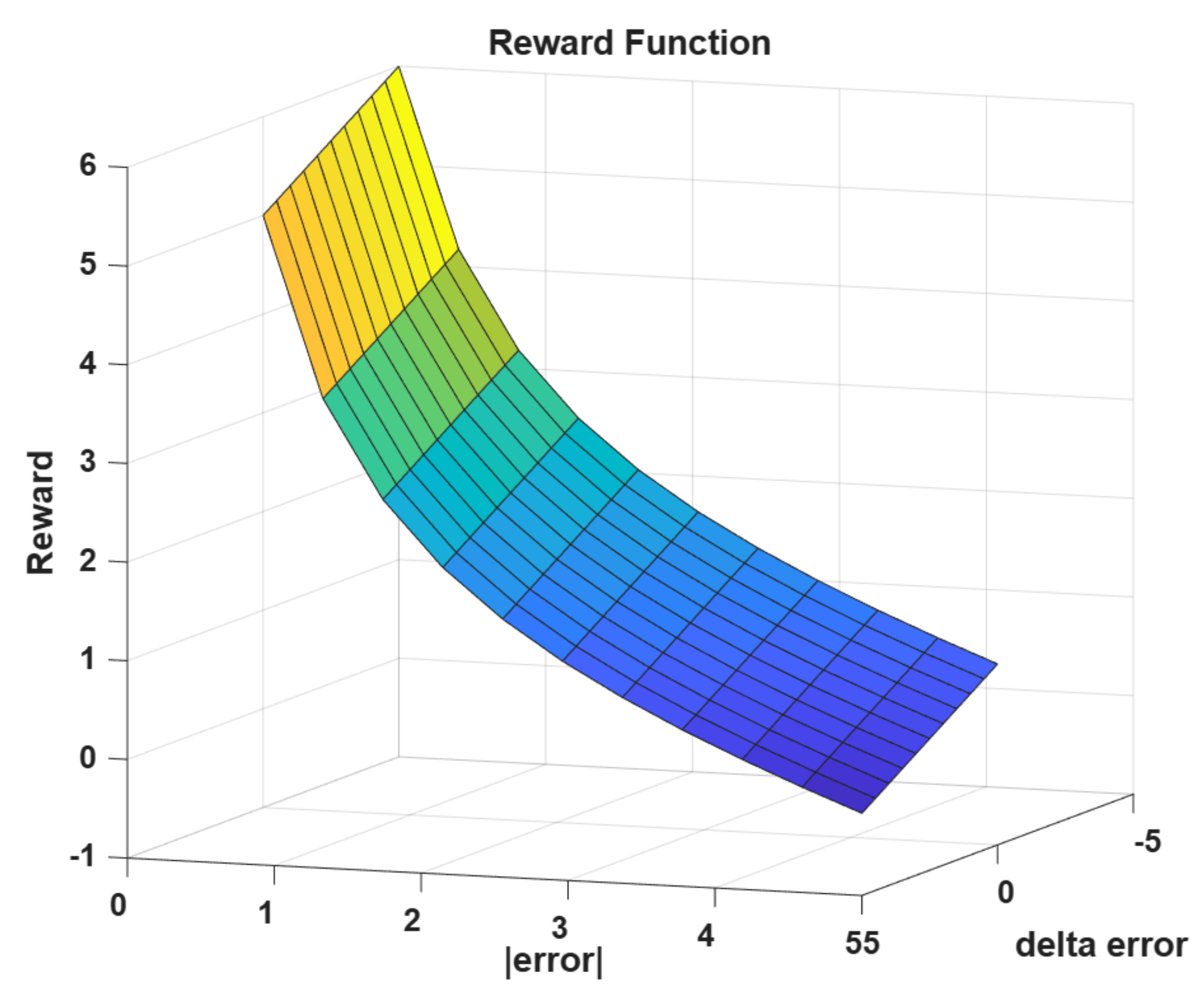
At each step, the agent selects one of the five actions. The action determines a force in applied to the surrogate model for state propagation. The scalar reward combines a term that depends on the absolute error and a term that depends on the change in absolute error between consecutive steps. Denote and . With two positive scalars g and and the normalization , the instantaneous reward reads
so that smaller error and decreases in error are rewarded, while increases in error are penalized. Equation (18) matches the plotted surface (reward as a function of and ) as shown in Figure 6, where the individual penalty and fitness function plots are shown in Figure 5. In training, the decrement term is realized by a finite difference of the absolute error tracked over time, with normalization by the error range:
Figure 5.
Reward and penalty elements utilized in the reward function construction.
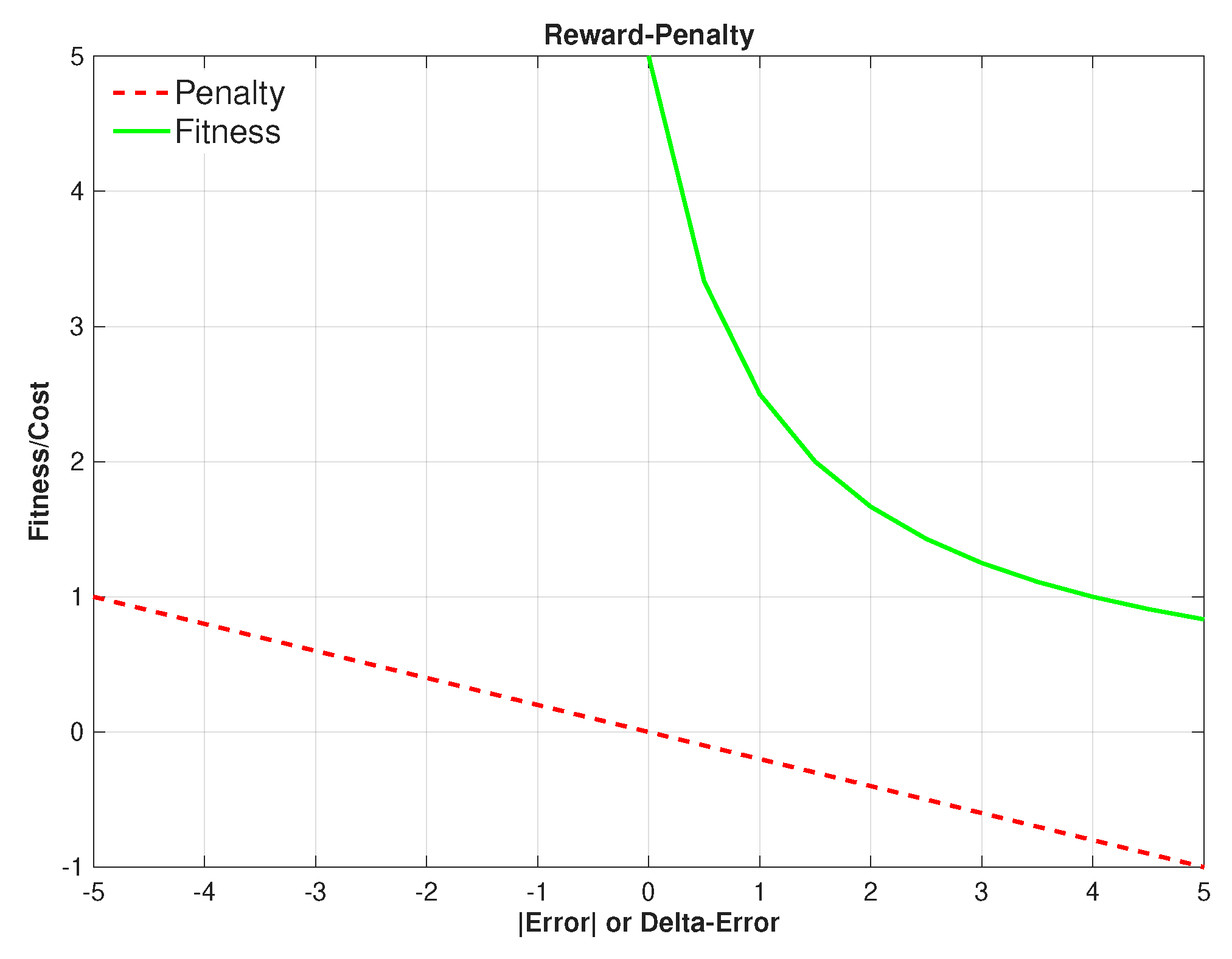
Figure 6.
Reward function utilized in the MBRL process.
Action selection follows -greedy exploration with exploration probability ; typical values used are (learning rate), (discount), and (exploration), and a scalar gain to scale the reward (reward amplification). The Q-update at step k is
where is a bounded shaping term that mildly penalizes actions incompatible with the coarse state region, and is its weight. This auxiliary term biases learning toward consistent actuation while preserving the Bellman target in the bracketed expression.
At the start of training ; a full tensor of Q-tables across episodes is retained for offline visualization. Unless otherwise specified, episodes begin from rest (, ) and the target position is drawn within the admissible range to expose the agent to a variety of setpoint locations; the state index is derived from the clipped error by (17). During training, the surrogate model exclusively advances the state. For the stitched piecewise model, five second-order local recursions are run in parallel and blended by triangular membership weights to produce the next predicted position; the resulting error is mapped to the next state by (17). For the NLARX model, the next predicted position is obtained by evaluating the nonlinear mapping on the regressor of two past outputs and inputs, with a one-step input delay; the predicted position then yields the next discrete state via (17). In both cases, no direct interaction with the true plant occurs during Q-learning rollouts. The Q-table progress as a heat map is depicted in Figure 7 and Figure 8 for the PLM and NLARX respectively. Filled contour plots of the Q-table illustrate how the value function evolves from the initial pre-convergence Q-function to the final convergence.
5. Performance Analysis
Closed-loop validation is conducted on the true nonlinear mass–spring–damper system after training the Q-learning agent with one of the two data-driven models (piecewise linear model, PLM, or nonlinear autoregressive model with exogenous input, NLARX). Each validation run consists of a single episode of length steps with sampling time s. The reference input is a unit position, , and the goal is to drive the measured position to rapidly with small transient deviation and minimal bias. The trained Q-table is held fixed during validation. Representative position responses under the two trained agents are shown in Figure 9. In each plot, the measured position, and the absolute tracking error are displayed to highlight convergence, transient behavior, and steady-state bias.
The performance metrics are considered as follows. Let denote the tracking error and the number of validation samples. The mean absolute error (MAE) and the standard deviation of the error (STD) are defined as . For a unit step reference, percent overshoot (PO) and settling time () are defined in the standard way:
with unless stated otherwise. The steady-state error (SSE) is evaluated over a terminal window and reported as a percentage of the reference magnitude, .
The principal validation metrics for the two trained agents are summarized in Table 1. Training sample counts refer to the data used to construct the respective data-driven model prior to Q-learning.
The PLM-trained agent exhibits markedly lower mean absolute error and substantially lower steady-state error relative to the NLARX-trained agent, indicating superior bias rejection around the unit setpoint and overall tighter tracking. Percent overshoot is slightly smaller for the PLM case, while the settling time is identical at approximately 7 s for both agents under the stated criterion. The standard deviation of the error is comparable across the two cases, reflecting similar residual fluctuations about the final value once the transient decays. From a data perspective, the PLM approach aggregates samples via five operating-point experiments to populate local linear dynamics across the range, whereas the NLARX approach relies on a single -sample experiment spanning the full input range, which results in a more compact data requirement but a larger steady-state bias in the reported validation. In qualitative terms, the desired performance consists of low overshoot, short settling time, and minimal steady-state bias while maintaining low error overall and modest training cost. The PLM results align more closely with these goals at the expense of larger identification data; the NLARX results illustrate a faster data-collection phase but increased bias and mean error in the tested scenario. The trade-off underscores that piecewise local linearization over a grid of operating conditions can yield high-fidelity behavior near the reference at the cost of multiple experiments, whereas a single global nonlinear regression reduces identification effort but may underfit key nonlinearities or exhibit bias under the tested reference transition.
6. Discussion
The results indicate that both data-driven models enable off-plant training of a discrete-action agent that achieves closed-loop tracking on the true nonlinear mass–spring–damper system. The piecewise linear model (PLM) yields lower mean absolute error and substantially reduced steady-state bias relative to the nonlinear autoregressive model with exogenous input (NLARX), at comparable overshoot and settling time. This behavior suggests that locally valid linear descriptions, blended across the operating range with fuzzy membership attributes, provide an effective basis for value iteration in the present task when the validation reference is a unit step.
A central trade-off emerges between prior knowledge and data demands. Construction of the PLM presupposes decisions about model order and about the placement of operating biases at which local models are identified. Such design choices encode valuable prior information about the plant, but that information is not always available for complex nonlinear systems or may be costly to obtain. In contrast, the NLARX route requires less a priori structure and concentrates data collection in a single experiment spanning the full input range. The observed increase in mean and steady-state error for the NLARX-trained agent reflects the well-known tension between model generality and bias: a compact global regressor fitted on a heterogeneous dataset may underrepresent regimes most relevant to the validation target, whereas locally fitted linear models emphasize fidelity near their operating regions. The comparison highlights that approaches requiring minimal existing knowledge are attractive and also challenging, particularly where safety or actuation limits restrict exploratory richness.
Several aspects of the learning formulation influence the reported performance. The discrete 100-state error index imposes a quantization of the value function that bounds achievable accuracy near the setpoint; finer partitions reduce quantization error but increase sample complexity. The five-action alphabet constrains the closed-loop authority and contributes to the observed overshoot; richer action sets reduce actuation quantization at the cost of a larger Q-table. The reward combines absolute error and its one-step change; this choice accelerates transient improvement yet can amplify sensitivity to short-horizon variability when the prediction model is imperfect. The hard-stop projection at the position limits ensures safety but introduces kinks in the closed-loop map; trajectories that graze the boundary can therefore exhibit non-smooth value updates, which the tabulated metrics do not fully reveal.
The fidelity gap between the identified model used for training and the true plant used for validation constitutes a primary source of residual bias. For PLM, model mismatch is dominated by interpolation across membership regions and by unmodeled cross-coupling between regimes; careful placement and shaping of the membership functions mitigate these effects. For NLARX, mismatch arises from regressor under-parameterization, choice of basis nonlinearity, and distributional differences between training and validation trajectories. Both models generalize from pseudo-random excitation to reference tracking, but the distribution shift from exploration to a deterministic setpoint task contributes to the steady-state deviations observed for the global model.
From a computational perspective, both models are light-weight at run time: PLM requires the update of a small number of second-order recursions and a convex combination, while NLARX evaluation reduces to a static nonlinear map on a short regressor. The primary cost lies in data collection and model fitting, which is higher for the PLM due to multiple operating-point experiments but lower for NLARX due to a single broad-range experiment. The reported outcomes therefore present complementary pathways: when modest prior knowledge about order and operating regions is available, PLM-based training delivers superior bias rejection; when such knowledge is scarce or the plant is difficult to segment, an NLARX-based route reduces up-front design effort at the expense of increased steady-state error in the present configuration.
The study remains subject to limitations. Performance is quantified for a unit step target; multi-step or trajectory tracking, disturbance rejection, and robustness to unmodeled friction changes merit separate assessment. The use of model-bypassed rollouts mitigates experimental risk but introduces model-induced bias in the learned value surface, which suggests examining on-line model adaptation or intermittently grounded updates with limited true-plant interaction. Finally, the discretized state–action setting provides clarity and stability for tabular learning but does not exploit potential smoothness of the value function; continuous approximators with constrained exploration may reduce quantization artifacts while preserving safety.
7. Conclusions
The study demonstrates that model-based reinforcement learning with data-driven models enables off-plant policy training for nonlinear regulation while containing experimental risk. A nonlinear mass–spring–damper with hardening effects and hard stops is addressed using two alternatives: a piecewise linear model assembled from operating-region identifications and a nonlinear autoregressive model with exogenous input learned from a single broad-range experiment. Tabular Q-learning on an error-indexed state space with a finite force alphabet produces controllers that achieve stable reference tracking on the true plant. A principal insight emerges: performance is governed by a fidelity–knowledge–data trade-off. Locally identified linear descriptions blended across the operating range tend to yield tighter regulation near the setpoint, provided that model order and operating regions are known or can be chosen sensibly. A global autoregressive description reduces prior structural assumptions and simplifies data collection, at the cost of increased residual bias under the tested reference. The error/discrete-state formulation and the reward combining magnitude and short-horizon reduction prove effective in practice and remain transparent to diagnose. The methodology is modular and transferable to other bounded-actuation systems subject to safety limits. Immediate extensions include adaptive refinement of the state partition, uncertainty-aware planning within the model loop, and limited on-plant fine-tuning to mitigate model–plant mismatch while maintaining safety.
Author Contributions
Conceptualization, M.P.S. and N.F.; methodology, G.G.J.; software, N.F. and G.G.J.; validation, G.G.J.; formal analysis, N.F. and G.G.J.; investigation, G.G.J. and M.P.S.; resources, M.P.S.; writing—original draft preparation, N.F., G.G.J., and M.P.S.; writing—review and editing, N.F., G.G.J., and M.P.S.; visualization, N.F. and G.G.J.; supervision, M.P.S.; project administration, M.P.S. All authors have read and agreed to the published version of the manuscript.
Funding
This research received no external funding.
Data Availability Statement
The original contributions presented in this study are included in the article, further inquiries can be directed to the corresponding author.
Conflicts of Interest
We declare that we have no financial and personal relationships with other people or organizations that can inappropriately influence our work; there is no professional or other personal interest of any nature or kind in any product, service, and/or company that could be construed as influencing the position presented in, or the review of, the manuscript entitled.
References
- Keesman, K.J. System Identification: An Introduction; Springer: Berlin, Heidelberg, 2011. [Google Scholar]
- Ljung, L. System Identification. In Signal Analysis and Prediction; Birkhäuser Boston: Boston, MA, 1998; pp. 163–173. [Google Scholar]
- Landau, I.D.; Zito, G. Digital Control Systems: Design, Identification and Implementation; Springer: London, 2006. [Google Scholar]
- Chen, C.W.; et al. Integrated System Identification and State Estimation for Control of Flexible Space Structures. Journal of Guidance, Control, and Dynamics 1992, 15, 88–95. [Google Scholar] [CrossRef]
- Nelles, O. Nonlinear System Identification. Measurement Science and Technology 2002, 13, 646. [Google Scholar] [CrossRef]
- Majji, M.; Juang, J.N.; Junkins, J.L. Observer/Kalman-Filter Time-Varying System Identification. Journal of Guidance, Control, and Dynamics 2010, 33, 887–900. [Google Scholar] [CrossRef]
- Kuo, C.H.; Schoen, M.P.; Chinvorarat, S.; Huang, J.K. Closed-Loop System Identification by Residual Whitening. Journal of Guidance, Control, and Dynamics 2000, 23, 406–411. [Google Scholar] [CrossRef]
- Pintelon, R.; Schoukens, J. System Identification: A Frequency Domain Approach; Wiley: Hoboken, NJ, 2012. [Google Scholar]
- Lee, H.; Huang, J.K.; Hsiao, M.H. Frequency Domain Closed-Loop System Identification with Known Feedback Dynamics. In Proceedings of the AIAA Guidance, Navigation, and Control Conference, 1995.
- Huang, J.K.; Lee, H.C.; Schoen, M.P.; Hsiao, M.H. State-Space System Identification from Closed-Loop Frequency Response Data. Journal of Guidance, Control, and Dynamics 1996, 19, 1378–1380. [Google Scholar] [CrossRef]
- Chinvorarat, S.; Lu, B.; Huang, J.K.; Schoen, M.P. Setpoint Tracking Predictive Control by System Identification Approach. In Proceedings of the Proceedings of the 1999 American Control Conference. IEEE, 1999, Vol. 1, pp. 331–335.
- Chiuso, A.; Pillonetto, G. System Identification: A Machine Learning Perspective. Annual Review of Control, Robotics, and Autonomous Systems 2019, 2, 281–304. [Google Scholar] [CrossRef]
- Cui, M.; Khodayar, M.; Chen, C.; Wang, X.; Zhang, Y.; Khodayar, M.E. Deep Learning-Based Time-Varying Parameter Identification for System-Wide Load Modeling. IEEE Transactions on Smart Grid 2019, 10, 6102–6114. [Google Scholar] [CrossRef]
- Brunke, L.; Greeff, M.; Hall, A.W.; Yuan, Z.; Zhou, S.; Panerati, J.; Schoellig, A.P. Safe Learning in Robotics: From Learning-Based Control to Safe Reinforcement Learning. Annual Review of Control, Robotics, and Autonomous Systems 2022, 5, 411–444. [Google Scholar] [CrossRef]
- Jaman, G.G.; Monson, A.; Chowdhury, K.R.; Schoen, M.; Walters, T. System Identification and Machine Learning Model Construction for Reinforcement Learning Control Strategies Applied to LENS System. In Proceedings of the 2022 Intermountain Engineering, Technology and Computing (IETC), 2022, pp. 1–6. [CrossRef]
- Farheen, N.; Jaman, G.G.; Schoen, M.P. Model-Based Reinforcement Learning with System Identification and Fuzzy Reward. In Proceedings of the 2024 Intermountain Engineering, Technology and Computing (IETC), 2024, pp. 80–85. [CrossRef]
- Ross, S.; Bagnell, J.A. Agnostic System Identification for Model-Based Reinforcement Learning. arXiv preprint arXiv:1203.1007 2012.
- Martinsen, A.B.; Lekkas, A.M.; Gros, S. Combining System Identification with Reinforcement Learning-Based MPC. In Proceedings of the IFAC-PapersOnLine, 2020, Vol. 53, pp. 8130–8135.
- Shuprajhaa, T.; Sujit, S.K.; Srinivasan, K. Reinforcement Learning-Based Adaptive PID Controller Design for Control of Linear/Nonlinear Unstable Processes. Applied Soft Computing 2022, 128, 109450. [Google Scholar] [CrossRef]
- Hafner, R.; Riedmiller, M. Reinforcement Learning in Feedback Control: Challenges and Benchmarks from Technical Process Control. Machine Learning 2011, 84, 137–169. [Google Scholar] [CrossRef]
- Sutton, R.S. Dyna, an integrated architecture for learning, planning, and reacting. ACM SIGART Bulletin 1991, 2, 160–163. [Google Scholar] [CrossRef]
- Moerland, T.M.; Broekens, J.; Jonker, C.M. Model-based Reinforcement Learning: A Survey. Foundations and Trends in Machine Learning 2023, 16, 1–118. [Google Scholar] [CrossRef]
- Watkins, C.J.; Dayan, P. Q-learning. Machine Learning 1992, 8, 279–292. [Google Scholar] [CrossRef]
Figure 1.
Process flow in Model-Based Reinforcement Learning.
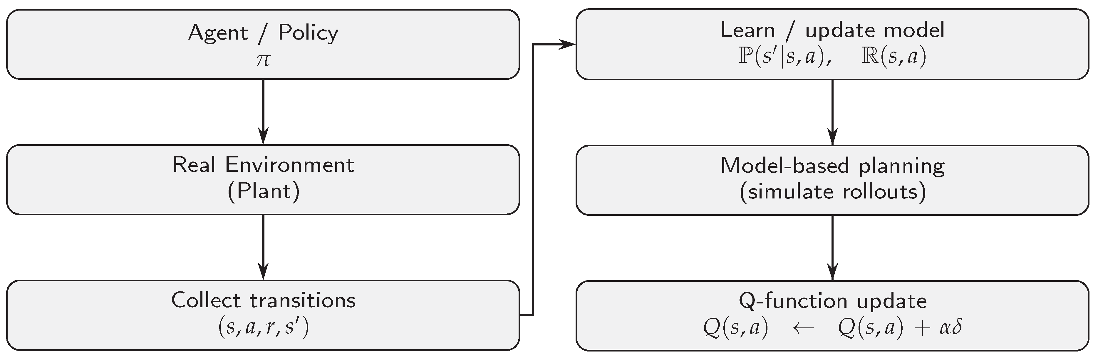
Figure 2.
Process flow of the MBRL experiments.
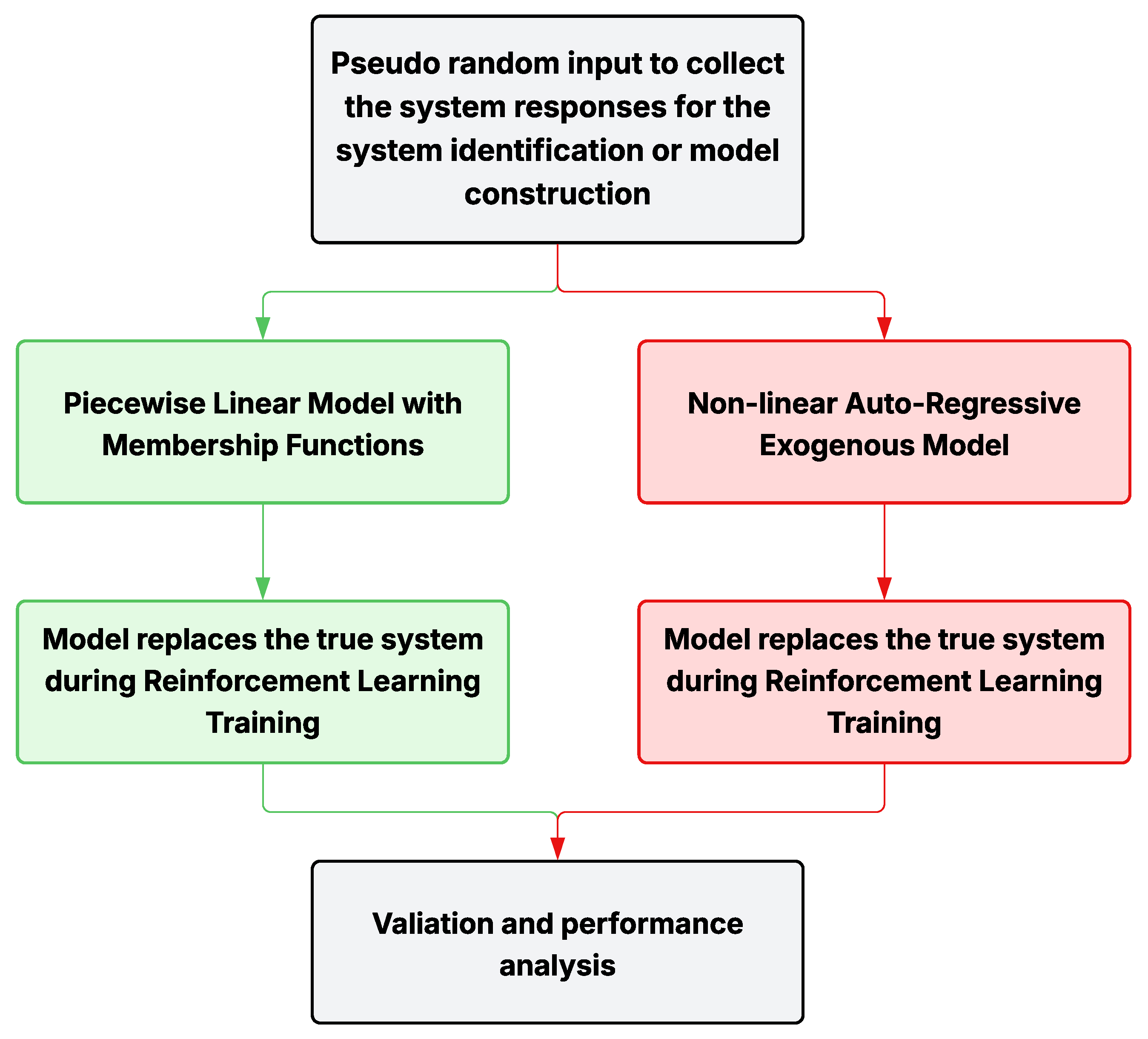
Figure 3.
Piecewise linear model validation at selected biases including the fitting metric.
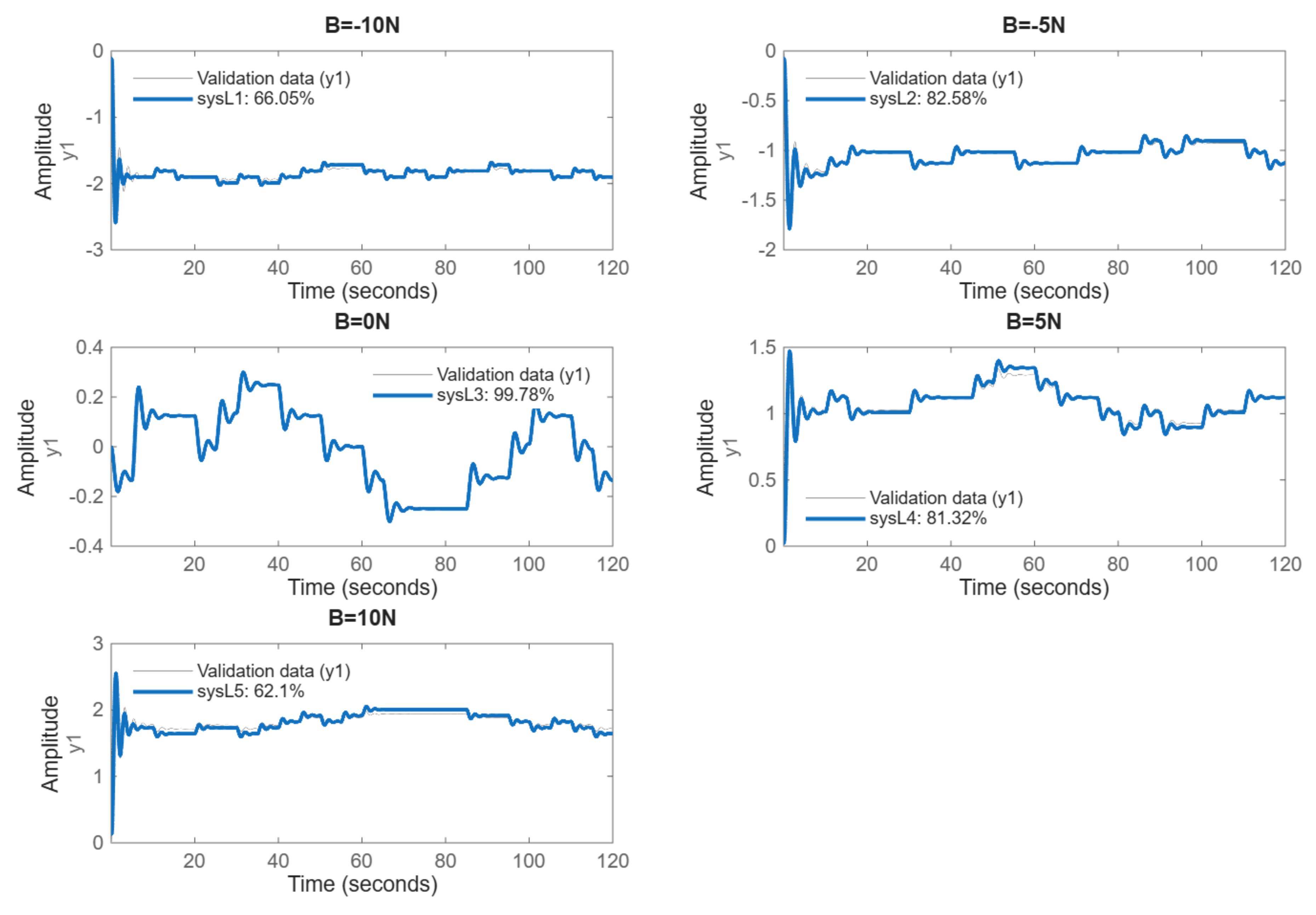
Figure 4.
NLARX model validation including fitting metric.
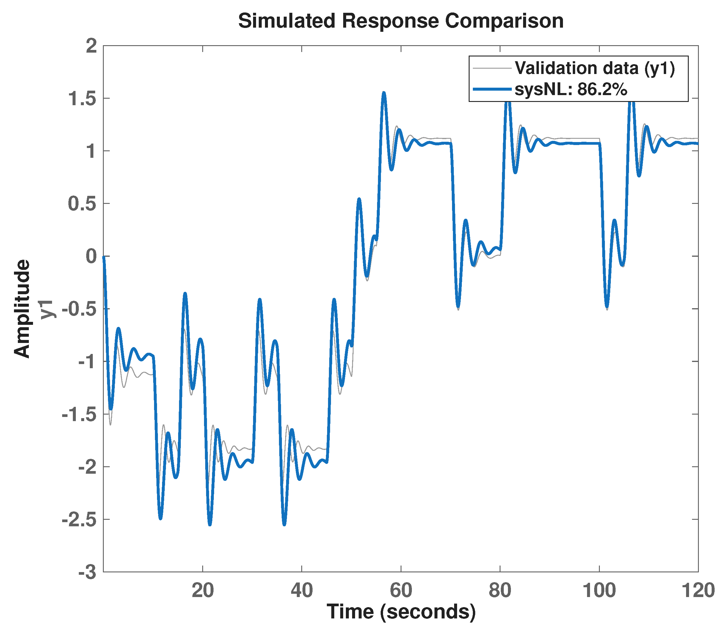
Figure 7.
Q-table learning status for PLM: (a) at the beginning (after single episode), and (b) at the end of all episodes.
Figure 7.
Q-table learning status for PLM: (a) at the beginning (after single episode), and (b) at the end of all episodes.
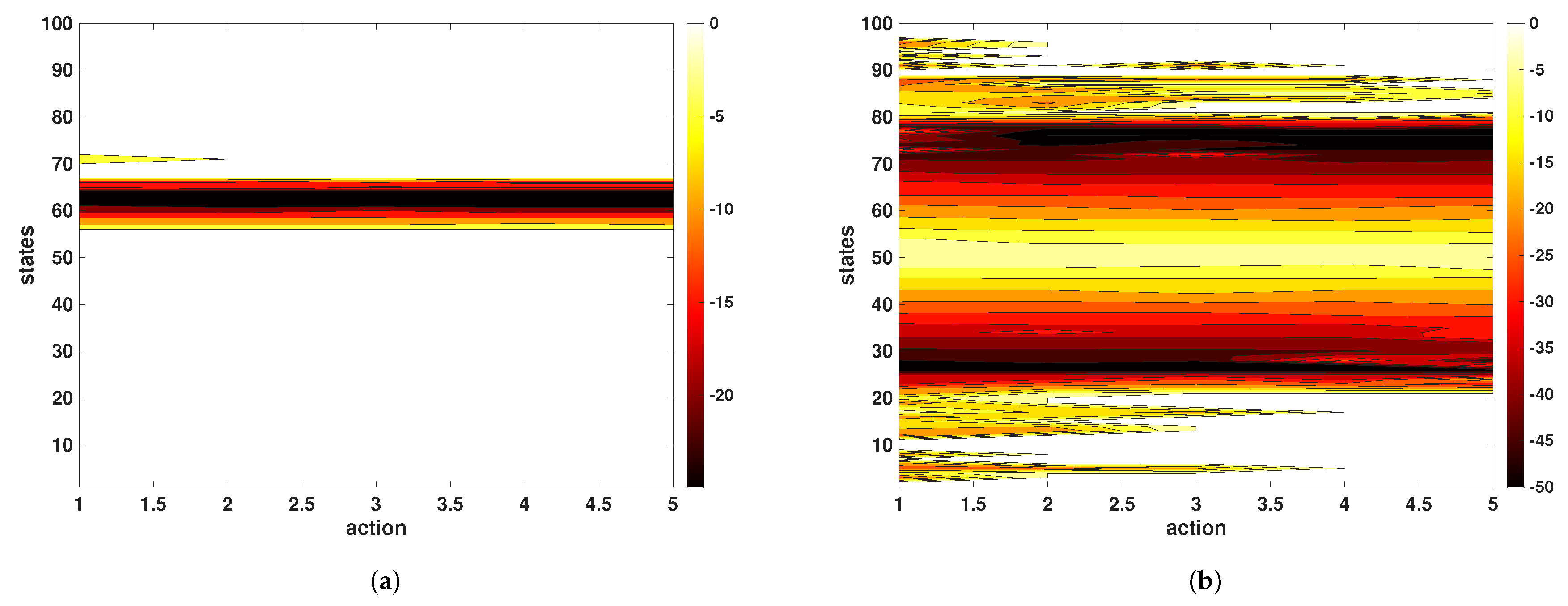
Figure 8.
Q-table learning status for NLARX: (a) at the beginning (after single episode), and (b) at the end of all episodes.
Figure 8.
Q-table learning status for NLARX: (a) at the beginning (after single episode), and (b) at the end of all episodes.
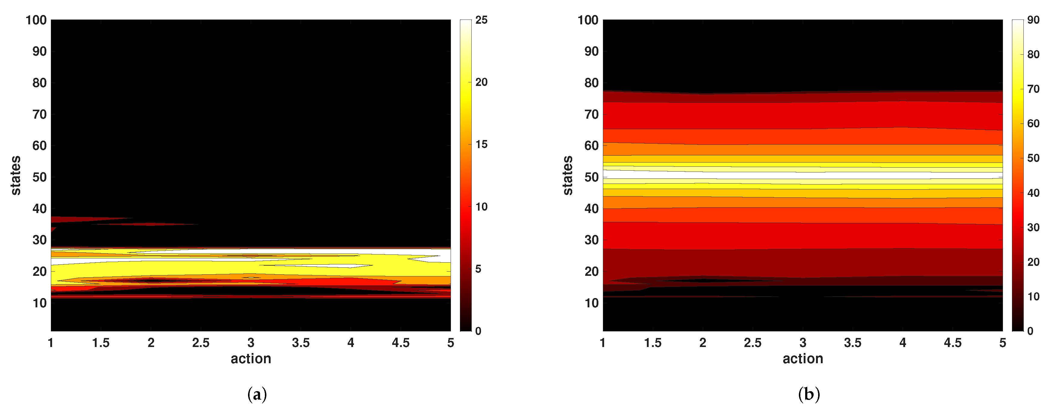
Figure 9.
Controller validation and closed-loop system response to unit reference: (a) tested on the agent from the PLM-MBRL, and (b) tested on the agent from the NLARX-MBRL.
Figure 9.
Controller validation and closed-loop system response to unit reference: (a) tested on the agent from the PLM-MBRL, and (b) tested on the agent from the NLARX-MBRL.
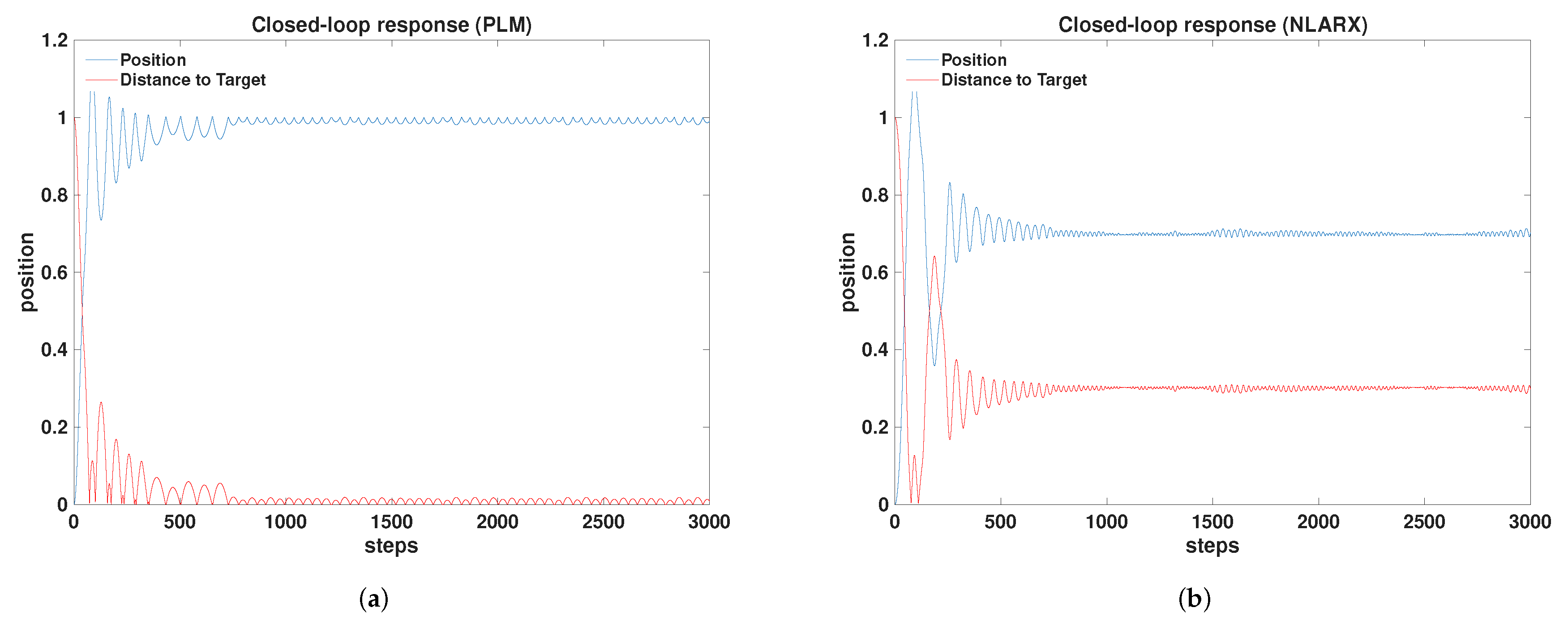

Table 1.
Closed-loop performance metrics on the true system for a unit reference ().
| Model | MAE | STD | SSE [%] | Overshoot [%] | Settling Time [s] | Training Samples |
|---|---|---|---|---|---|---|
| NLARX | 0.31 | 0.09 | 30 | 12 | 7 | 12,000 |
| PLM | 0.03 | 0.10 | 3 | 10 | 7 | 60,000 |
Disclaimer/Publisher’s Note: The statements, opinions and data contained in all publications are solely those of the individual author(s) and contributor(s) and not of MDPI and/or the editor(s). MDPI and/or the editor(s) disclaim responsibility for any injury to people or property resulting from any ideas, methods, instructions or products referred to in the content. |
© 2025 by the authors. Licensee MDPI, Basel, Switzerland. This article is an open access article distributed under the terms and conditions of the Creative Commons Attribution (CC BY) license (http://creativecommons.org/licenses/by/4.0/).
Copyright: This open access article is published under a Creative Commons CC BY 4.0 license, which permit the free download, distribution, and reuse, provided that the author and preprint are cited in any reuse.


