
Submitted:
09 August 2025
Posted:
11 August 2025
You are already at the latest version
Abstract
The growing reliance on autonomy in uncrewed aircraft systems (UAS) necessi-tates a real-time solution for assured contingency landing management during in-flight emergencies. This paper presents a novel gradient-guided search algorithm for risk-aware emergency landing trajectory generation with a wing-lift UAS loss of thrust use case. This framework integrates a compact four-dimensional discrete search space with aircraft kine-matic and ground risk cost. A multi-objective cost function is employed, combining flight envelope feasibility, optimal descent, and overflown population risk terms. To ensure discrete search convergence, a constrained hypervolume definition is introduced around the destination. A holding pattern identification algorithm is defined to minimize risk during the necessary flight path angle constrained descent to final approach. Planner effectiveness is validated through randomly generated case studies over a region of Long Island, NY under steady wind conditions. Benchmark comparisons with a 3D Dubins solver demonstrate the approach’s improved risk mitigation and acceptable real-time com-putation overhead. Future development will focus on integrating collision avoidance into the discrete search-based landing planner.
Keywords:
assured contingency landing management
; advanced air mobility
; discrete search
; real-time risk mitigation
; path planning
1. Introduction
Advanced Air Mobility (AAM) will support a combination of Uncrewed Aircraft Systems (UAS) and larger air taxi platforms flying low over densely populated urban areas. Although electric Vertical Takeoff and Landing (eVTOL) aircraft are expected to offer a Lift-Cruise configuration [1,2], a variety of conditions ranging from propulsion module failure to unexpectedly low battery energy or fuel can render any aircraft unable to remain aloft long-term. A Lift-Cruise eVTOL with low battery energy can safely fly longer, with more margin, if it remains in cruise configuration rather than converting to vertical flight. Whether operating in wing lift (cruise) mode due to a fixed-wing configuration or due to a low energy or eVTOL propulsion unit failure condition, a contingency landing plan can be safest for aircraft, any onboard occupants (if present), and people on the ground below when this aircraft relies on wing lift throughout a stable planned descent to land on a nearby runway. Because aircraft can glide without consuming fuel in wing lift mode, it is the most energy efficient configuration. Gliding is also feasible regardless of which propulsion unit fails. Therefore, this paper models the aircraft in wing lift mode during contingency descent to landing. While this work is motivated in part by larger AAM platforms such as eVTOL air taxis, the underlying approach is equally applicable to smaller-sized UAS capable of operating in wing-lift mode. The algorithm’s reliance on aerodynamic gliding and discrete ground risk data enables autonomous onboard planning for drones conducting logistics, surveillance, or emergency response missions - applications that are becoming increasingly common in densely populated areas [3,4,5].
During urgent or emergency landings, the distressed aircraft has priority over other traffic but must deal with whatever winds and weather are present. This work therefore focuses on consideration of steady wind and flight envelope margin and appropriately assumes other aircraft will avoid collision with the distressed aircraft as it lands. Path planning for urgent or emergency landing requires a four-dimensional solution that meets strict spatiotemporal constraints and minimizes safety risks. Along with implementation of degraded aircraft performance constraints for flight safety, ground risk is quantified by employing discrete population census data in this paper.
Fixed-wing (wing lift/cruise configuration) aircraft have non-holonomic motion constraints that require maintaining forward motion at a minimum (stall) speed and limiting turn radius. Urgent landing descent paths must avoid obstacles, minimize risk, and align with suitable runways while accounting for steady winds in planning and adjusting to actual variable winds during plan execution. There are several methods for aircraft path planning. However, not all of them are suitable for constrained minimum-risk path planning in complex environments. For instance, although they are fast to compute, geometric solutions such as Dubins paths [6,7,8] solely incorporate path length and curvature metrics. Despite the success of optimal control (OC) and model predictive control (MPC), these methods suffer from initial guess dependency, non-convergence, and low computational efficiency in complex environments [9,10,11,12,13]. In addition, it is difficult to adapt inherently discrete ground risk metrics to OC and MPC as solutions may become stuck at local minima that may not meet feasibility constraints. Similarly, Hamilton-Jacobi-Bellman (HJB) reachability does not scale efficiently due to the curse of dimensionality [14]. Moreover, the HJB value function requires spatial continuous differentiability [15], a requirement that discrete ground risk cost violates. Even though such metrics can be approximated by projecting data onto smooth hyperplanes (e.g., Fourier series expansion) this task increases complexity while reducing the data resolution. Note that dynamic cost metric updates such as ground risk values derived from mobile phone activity [16] and real-time ground traffic data [17] render data projection computationally unaffordable for real-time risk quantification as part of contingency planning.
Tree-search-based path planners are well-suited for diverse, discrete cost metrics such as ground risk. As example related works, Ref. [18] applies a modified A* algorithm to find a shortest feasible path. In [19] and [20], Monte Carlo Tree Search was exploited to plan UAS flight paths. A rapidly-exploring-random tree (RRT) was used in [21,22,23] to safely navigate a space with obstacles. Ref. [24] used pre-calculated maneuvers for emergency landing planning for a gliding aircraft. Markov Decision Process (MDP) formulations in Refs. [25,26] focused on uncertainty in aircraft performance and prognostics-based margin, respectively, in emergency landing planning. Tree-search over feasible post-failure maneuver primitives for emergency landing planning was proposed in [27] as an extension of a Dubins-based geometric solver in [28]. A three-dimensional A* variant in [29] balanced flight path and landing site risk but faced significant complexity challenges when path length was substantial. This work advances previous search-based and MDP approaches by integrating risk, kinematic, and flight envelope constraints within a solver that efficiently generates feasible long-distance 4D landing paths. This paper’s approach accounts for operational altitude ranges with a minimum-risk loitering approach and wind effects while maintaining a compact heading-constrained search space.
This article is a revised and expanded version of a paper entitled Gradient Guided Search for Aircraft Contingency Landing Planning [30] which was presented at the IEEE International Conference on Robotics and Automation, Atlanta, USA, 19-23 May 2025. The discrete search contingency landing planner in this paper adopts a priority queue and operators inspired by the Theta* search algorithm [31] to accommodate flight envelope constraints as a function of steady wind. By fusing feasible path and population risk cost metrics, the presented method simultaneously considers safety of the landing (e.g., path margin) and risk due to a distressed aircraft passing over an urban population. The multi-objective cost function forms a gradient field that significantly reduces state-space exploration thus to minimize computational overhead to support real-time implementation. A constrained four-dimensional (4D) position and heading volume around approach fix is introduced to guarantee search convergence. Since ground risk is negligible at high altitude, the planner incorporates a three dimensional (3D) Dubins path solver with a holding point identification scheme to efficiently generate a path to a minimum-risk holding pattern that dissipates altitude. The algorithm’s effectiveness is demonstrated through use cases under steady wind at different initial states. Search-based planning results are benchmarked against 3D Dubins path solvers, evaluating overflown population risk, deviations from optimal gliding trajectories, and computational overhead. The key contributions of this work include:
- Efficient and feasible contingency landing planning with a compact 4D discrete search framework guided by a cost function with a constraint margin gradient field.
- A constrained hypervolume definition around an approach fix to ensure discrete search convergence.
- A real-time minimum-risk aircraft holding pattern placement algorithm and its integration into contingency landing planning.
- Assured contingency landing plan generation within a prescribed time limit.
This paper is organized as follows. Section 2 introduces fundamental concepts that this work builds upon including gliding flight envelope determination of an aircraft in fixed-wing mode, reachability, and geometric path planning. Section 4 presents the key components of the contingency landing planner such as the building blocks of the gradient-guided search incorporating flight feasibility and landing risk assessment with a convergence guarantee. Below, preliminaries and methodology are followed by use case studies over a Long Island, NY region with a Cessna 182 fixed-wing performance model serving as a surrogate to a four-passenger AAM aircraft operating in fixed-wing mode.
2. Preliminaries
This section summarizes the principles of fixed-wing aircraft flight, reachability, and geometric path planning. These concepts are essential for understanding and developing emergency landing planning procedures.
2.1. Fixed-Wing Aircraft Performance
A fixed-wing aircraft is exposed to three fundamental forces [32]: aerodynamic, gravitational, and propulsive, as shown in Figure 1.
High wing lift L to drag D ratio is the key to efficient fixed wing or "cruise" mode eVTOL flight [33]. Lift is mainly produced by the pressure difference between upper and lower wing surfaces and requires forward flight above a minimum stall speed. In cruise flight, forward thrust T generated by propulsion units must counter drag D while lift L balances total weight W. The four primary forces () define flight path angle , the angle between the ground velocity and the horizontal plane, with in level flight. Aircraft course angle, denoted by , is the angle between North and the horizontal projection of .
Best glide flight path angle in forward flight (1) defines the most shallow descent possible without thrust. It is defined by the fixed-wing aircraft nonlinear equations of motion where and denote state and control input vectors, respectively.
Best glide for a two-minute standard constant radius turn under steady wind conditions is as formulated in Equation (2) where bank angle . An additional inequality constraint [34] on maximum bank angle limits the maximum load factor to meet structural integrity constraints.
The best-glide angle is important for any emergency situation where an aircraft needs to descend rapidly, even if the engines are still operational but delivering reduced maximum output.
A good landing begins with a good approach, so it is important to define a stabilized approach speed. Wing flaps are extendable only below maximum flap extended speed . The steepest flight path angle for straight gliding (3) and turning (4) flight are identified to assure airspeed is upper bounded by .
The steepest gliding angle for turning is per Equation (3) where .
The best-glide and steepest descent flight path angle pair of a Cessna 182 (C182) [35] are defined as functions of wind speed and direction , and obtained as in [17]. Given no forward thrust (), best-glide angle represents the shallowest gliding angle an aircraft can fly at without stalling. While aerodynamically efficient, this angle is susceptible to stall due to disturbances such as wind gusts. Conversely, flying at steepest glide angle requires a higher approach speed, leading to a longer deceleration path. To balance safety and efficiency during emergency approaches, flight path angle is defined per Equation (5) that lies halfway between and . offers an optimal safety margin. This value can be adjusted to provide flexibility in the safe landing path descent profile.
For clarity, flight path angle notation is simplified by omitting their input arguments, i.e., . Note that all flight path angles are functions of steady wind conditions as used to define aircraft turn radius R per Equation (6) [33] for path planning.
Here, g and are gravitational acceleration and wing bank angle, respectively.
2.2. Reachable Footprint
For emergency landing, potential landing sites must be identified within a reachable area. This area, known as the reachable footprint [28], is determined by the aircraft’s capabilities and the specific emergency. For example, a complete loss of thrust limits the reachable footprint to the gliding range, while a medical emergency prioritizes nearby landing sites that are also close to healthcare facilities to minimize total transit time. Various methods have been proposed to determine the reachable area for distressed aircraft landing. Aircraft dynamics analysis [36,37], optimal control theory [38], Hamilton-Jacobi methods [39,40], and attitude optimization [41] have been employed with different cost/benefit trade-offs. In this paper, reachability of the target destination is assumed confirmed to focus this research effort on path planning to a designated site.
2.3. Geometric Aircraft Path Planning
The Dubins path [6] provides a geometric solution for transitioning between two states while respecting a minimum turning radius constraint. Originally formulated for two-dimensional paths, assuming constant altitude, this solution has been extended to three-dimensional aircraft path planning applications [8,42,43]. The literature offers several contingency landing management frameworks with Dubins paths. Ref. [7] modified the kinematic model of Dubins paths to include transient effects such as translational and rotational acceleration in emergency path planning. Ref. [28] extends Dubins paths by incorporating real-time updates for dynamically feasible landing plans under degraded aircraft performance. Dubins path and RRT* are fused in [44] to create emergency landing procedures. Ref. [17] incorporated datalink and Dubins path to coordinate distressed aircraft and ground traffic for road-based emergency landings.
Conventional Dubins path solutions are formed by an initial minimum radius turn segment, a final minimum radius turn segment, and a straight segment connecting tangents of the initial and final turns. There are four options for turn-straight-turn type of paths: right-straight-right (RSR), right-straight-left (RSL), left-straight-right (LSR), and left-straight-left (LSL). Dubins [6] also defined solutions with intermediate turns (RLR and LRL) but these are not practical for long distance traversals between arbitrary configurations. Most Dubins solvers typically evaluate all four path types and select the shortest assuming constant velocity. Path geometry and length derivations can be found in [32].
To enhance discrete search-based path planning, the proposed algorithm incorporates 3D Dubins path solutions. For instance, Dubins paths can be employed to establish a connection between an initial emergency state and a designated holding point, as well as to link a discrete search-generated trajectory to final approach to the landing runway. Also, S-turn Dubins paths [28] are employed for benchmarking.
Aircraft state is defined as a tuple where , , , and respectively correspond to latitude, longitude, altitude above mean sea level (MSL), and course angle. The symbols and denote valid sets of latitude and longitude. The set of all possible aircraft states are defined per Equation (7).
Let the initial and final states respectively be and . A contingency landing path consists of a sequence of states from to where . A set of Dubins path solutions between arbitrary states and are denoted by per Equation (8).
The shortest Dubins solution is defined in Equation (9) where is the length of path .
Note that ; thus , can be an empty set if is unreachable given .
3. Problem Statement
Ensuring a safe and feasible contingency landing for fixed-wing aircraft in emergency scenarios is a critical problem that demands both efficiency and reliability. The objective of this paper is to present and analyze a contingency landing planner that minimizes risk to the overflown population while ensuring timely definition of a feasible path. This problem presents several key challenges. First, the feasibility of the landing path is constrained by the distressed aircraft’s flight envelope, necessitating a careful assessment of its aerodynamic limitations given degraded performance. Second, minimizing risk along the trajectory requires accurate evaluation and incorporation of risk data. Another fundamental challenge lies in the computational complexity of search-based path planning. The need to explore a continuous search space with theoretically infinite extent complicates real-time decision-making and solution convergence guarantees. This trade-off between runtime efficiency, search completeness, and trajectory risk must be carefully managed to ensure a practical implementation. For this study, the following assumptions are made. First, designated landing sites are assumed to be within the aircraft reachable footprint. Second, this paper assumes a known steady wind throughout the descent to landing.
4. Methodology
This section introduces the contingency landing planner and its building blocks including a search-based path planning algorithm, a solution identification criterion, and a method to define a minimum-risk holding pattern.
4.1. Contingency Landing Path Planning
Because a Dubins solution is purely geometric, risk metrics cannot be considered. A low-flying aircraft in distress poses risk to an overflown population. However, an aircraft at high altitude poses negligible risk to people on the ground below because it will fly well past its current position before reaching the ground even in a steep descent. Discrete search with a population risk metric is therefore only useful when the aircraft descends below a crossover altitude . The handling of high and low altitude cases is illustrated in Figure 2.
In a low-altitude emergency, a discrete search planner generates a low-risk, energy-managed path from the initial emergency state to the final search state . Final search state is constrained to lie in a predefined hypervolume around . Then, a final turn to join a final approach path to touchdown state is computed with a 3D Dubins path considering as a fly-by waypoint. Note that the exact initial and final states of the Dubins path for the final turn are respectively computed by the Dubins path solver between and as well as and , to ensure feasibility with respect to aircraft dynamics and kinematic continuity. Formally, a low-altitude solution is defined as:
In a high-altitude emergency, the distressed aircraft must descend at a flight path angle near before initiating an approach to landing. Altitude dissipation is achieved by defining a circular holding pattern with inbound state and outbound state . The planner identifies the optimal holding pattern location using a utility function specified below. It connects to with the shortest Dubins path . The holding pattern is traversed until reaching where discrete search is initiated to find a low-risk low-altitude landing path to . A high-altitude solution can be expressed as:
A transition case arises if yet is unreachable above . Similar to high-altitude cases, a Dubins path is generated from to . The crossover state at the crossover altitude on the path to is identified. The search-based planner then generates a low-risk path from to . Then, the solution is finalized with a 3D Dubins path . Solution of a transition case is given by:
4.2. Search-Based Path Planning
An aircraft flight envelope defines its safe operating limits. These limits include but are not limited to stall for controllability, load factor and maximum airspeed for structural integrity. Let degraded aircraft flight envelope be defined as:
For a given aircraft flight envelope , , and , the search space per Equation (7) can be identified using a reachability method. In this study, is an infinite, continuous, and non-Euclidean space where the distance between arbitrary states are geodesic distances. Feasible actions for transition from a parent state to successor states are given by where is the branching factor. Each action is composed of course angle change , path segment length which is great-circle distance between the parent and successor state ℓ, and optimal straight gliding and turning flight path angles along segment and given a known steady wind.
where is a set of feasible course angle changes. The set of all feasible actions is per Equation (15) where .
For a given aircraft flight envelope , set of actions , initial and goal states and , state cost function , and steady wind with magnitude and direction , the 4D search-based path planning problem is formulated as in Equation (16) where is a non-ascending emergency landing path solution.
4.3. Feasible Actions
The action set must consist only of feasible actions considering potentially degraded flight envelope constraints. For example, while symmetrical lateral maneuverability can be used for left and right turns considering airspeed and load factor for a single-engine aircraft experiencing loss-of-thrust, asymmetrical course angle rate limits will be present for aircraft with deteriorated lateral controllability caused by conditions such as control surface jam [45], structural damage [46], and uneven icing [47]. The minimum segment length for a given arbitrary set of course angle changes is further defined below.
A sketch of sequential turns in the horizontal plane is shown in Figure 3. The minimum segment length that can accommodate sequential turns between state and is expressed by Equation (17). When expanding state , the next state and action are unknown; hence, can be substituted by the highest possible course change value to ensure feasibility.
The search algorithm uses an adaptive segment length (18) that reduces search resolution at higher altitudes where ground risk is minimal to improve real-time performance. This function uses , the altitude at , , the floor altitude change at the minimum segment length, and , the rate of segment length change per unit altitude.
Per Equation (5), and are determined within for given steady wind conditions. Therefore, a feasible action at state s is a function of wind speed and wind direction .
4.4. State Expansions
Successor states are generated by expanding parent states. A successor of parent s resulted from j-th feasible action of s is denoted by . Course angle of a successor state is
where and . The operator wraps an angle at . Coordinates of a successor state are computed by using World Geodetic System 1984 (WGS84) [48] model per Equation (20). Let be an operator such that . Simply, is a function that returns the destination coordinates given a reference state and action variables.
The altitude of the successor state (21) is computed considering turning and straight gliding traversals where .
Turning traversal is denoted by and calculated as in Equation (17). For convenience, the transition model is specified to apply an action to a state, which composes relations (19)-(21). The set of successors for parent state s is
Reciprocally, the parent of a successor state is .
4.5. Cost Functions with a Constraint Margin Gradient Field
The path planning cost function is constructed by four distinct terms: (1) a gradient function to prioritize state expansion with an optimal descent path angle, (2) a gradient function to guide search toward the target location, (3) a gradient function that guides search toward the desired course angle as the target location is approached, and (4) a term that discourages flight over densely populated urban areas. The total cost of a state is given in Equation (23).
Here, , , and are respectively optimal descent, direct distance, course angle, and population cost functions. Terms are weight coefficients while is an adaptive weighting factor. First, common terms used in cost functions are introduced. An approximate shortest path length to the goal is calculated based on a combination of turn and straight sections.
The function represents the great-circle distance from state s to , where returns the bearing angle between two states. The remaining best-glide range given the altitude loss from s to is defined as:
States with indicates unreachability and are pruned from further expansion. is defined as an approximate optimal distance to be flown to descend to goal altitude from initial altitude at optimal glide slope initially estimated based on the relative wind between and .
4.5.1. Optimal Gliding Cost
Two cost functions are employed to encourage progress toward the goal state region. The first function, (27), prioritizes the necessary altitude loss to reach the goal state. It serves as a measure of how efficiently the estimated total path length (the first two terms in the numerator) compares to the optimal descent path length. Consequently, it penalizes deviations from the optimal path length caused by deviation from the optimal flight path angle using the heuristic .
Here, is the total path length leading to s as a function of either state s or time t to reach s per Equation (28).
The cost is proven bounded per Lemma 1.
Lemma 1.
For a non-ascending landing path with , and an aircraft whose optimal glide angle satisfies , the cost function is bounded within the closed interval , .
Proof
(Proof of Lemma 1). The boundedness of can be established by analyzing the limits of , given that is a constant. Given the path slope , , a feasible landing path cannot exceed the best-glide range ; hence, the upper bound is:
Defining and substituting into the expression for , one obtains:
Given aircraft flight envelope with , it follows that:
Thus, is found. Next, the lower bound is examined. The quantity attains its minimum if and only if the initial and goal states coincide in latitude and longitude, i.e., . Given these conditions, and , leading to:
By equations (31) and (32), is found upper bounded by 1. Noting that is non-negative due to the absolute value term in its definition, it is concluded that:
Thus, is bounded within the closed interval , completing the proof. □
4.5.2. Direct Distance Cost
Using only ensures the path follows the optimal length using a heuristic, but it can lead to wasted potential energy by expanding nodes away from the goal, particularly in high-altitude emergency cases. To address this, a second function, , a heuristic estimate for the shortest path to the goal normalized by , is introduced per Equation (34). This function prioritizes states that are closer to the goal regardless of their descent profile.
Due to reachability limitations, the optimal flight path angle cannot be determined per Equation (5) if . In such cases, a shallower flight path angle - optimal for the specific emergency scenario - must be used to ensure reachability such that . Therefore, the condition inherently guarantees the boundedness of on closed interval , eliminating the need for a separate proof.
By weighting and , prioritization of expanding states towards the goal and establishment of the optimal descent profile are balanced. To achieve this balance, upper and lower bound radii around , respectively and , are specified to calculate to limit outward branching. Equation (35) defines while is a predetermined constant.
The weighting factor is
Equation (36) guides state expansion toward by adjusting the influence of and based on the state’s location in the search space. Specifically, according to Equation (23), when s is farther than from , is set to zero, preventing outward branching and conserving excess altitude. This allows the aircraft to later use its potential energy to navigate around densely populated areas. Conversely, when s is closer than to , is eliminated, prioritizing the optimal descent path by managing altitude loss.
To facilitate further analysis, let be:
Now, the boundedness of is established in Theorem 1.
Theorem 1.
The weighted sum of and is bounded within the closed interval , .
Proof of Theorem 1
By Lemma 1, is bounded within . Additionally, by definition, both and are constrained within . Since is a convex combination of these bounded functions, it follows that remains within , . The constant weights and do not alter the boundedness of the linear combination. □
Figure 4 demonstrates the evolution of during path planning. The vector field visualizes the gradient of , , indicating the preferred direction of state expansion.
Initially, in the leftmost figure where NM, the vector field around state s points away from the goal state. This outward direction of state expansion occurs as forms a repellent, high-cost region around goal state due to . As the path planning progresses, the search captures and follows the optimal decent path as in the second and third figures from the left. Finally, it converges toward by following the minimum cost isoline as depicted in the rightmost figures. If the initial altitude were set lower, the minimum cost region would lie between and due to , leading state expansion immediately toward .
4.5.3. Course Angle Cost
The costs and enable search to reach the goal region yet they do not reward the desired course angle. It is challenging to match the exact target course with a discrete search. Explicitly incorporating the course angle difference in a cost function would eventually enforce states to only expand parallel to the goal course which impedes necessary turns to match the goal location. Thus, a course angle cost that represents the preferred direction for approaching the goal state in lieu of exactly matching the landing runway course angle is proposed.
A unit normal vector represented in a North-East-Down (NED) coordinate system and aligned with the target course is used to partition the cost map into regions of higher and lower cost per Equation (38) where is the transformation operator from geodetic to NED coordinate system.
It should be noted that the vector operations in Equation (38) must be in a local coordinate system to eliminate asymmetrical gradient field with respect to due to the Earth’s curvature. The scalar product in Equation (38) evaluates the projection of the vector from an arbitrary state s to onto . A value of zero indicates that s lies on the line perpendicular to that passes through , bisecting the search map with a vertical plane. Such states require a turn to align with the final course, a common practice in airport traffic patterns for general aviation aircraft. States with are located in the region behind the bisecting line and require a course change of less than to reach the goal. Conversely, states with are penalized, as they necessitate a course angle change greater than to align with the landing site. Equation (38) is exploited to further define the course angle cost per Equation (39) where is a normalization constant to ensure the cost is bounded on the closed interval . The scalar product term is multiplied by distance terms to ensure that distant states can be explored in any direction, while nearby states are restricted to the region behind the bisecting line. The operator is introduced to zero out the course angle cost of states with .
The normalizer can easily be determined based on the maximum course cost value in the search space per Equation (40).
Overall, the operator ensures a lower bound of zero while normalizes to the upper bound to one, simplifying the need for a boundedness proof for on the closed interval .
An illustration of Equation (39) for is shown in Figure 5. The green arrow points in the goal course angle direction, and the vector field of encourages the search algorithm to expand states toward regions where , enabling a feasible final approach.
The function alone is insufficient to guide the search to the solution, as it only provides guidance for one half of the horizontal cost map. However, stacking on top of and alters the gradient field direction in the vicinity of the goal state, allowing state expansion in the right direction.
4.5.4. Population Cost
Population cost is computed by integrating the overflown population density over time. Let the population density function be . The function is reformulated as a function of time for a known state per Equation (41), where ∘ is the composition operator. In this paper, the population and land area dataset shared by the U.S. Census Bureau [49] is utilized to obtain population density as a function of time which will be denoted by for convenience. For population risk estimation, wind effect is ignored; thus, .
To reflect true population risk, a weighting function (42) is introduced to penalize under a lower altitude path.
Here, the crossover altitude is used for the ceiling altitude for population risk consideration. Therefore, population risk is not taken into account for path planning above .
In case of an emergency, the population residing under a given destination is not a factor as the aircraft is supposed to be approaching and landing at an airport runway in this work. Thus, the impact of population risk is reduced proportionally to the remaining traversal using a quadratic cost 43.
Time t is the input argument to Equation (28) for integration purposes.
Let the cumulative overflown population risk to reach from s in flight time t be the integration of weighted (41) with respect to time per Equation (44).
Here, the flight time t is estimated by . The boundedness of depends on the proper scaling by (45).
Per Equation (45), the population risk is time averaged and normalized by the upper bound of the weight product and maximum population density within the search space (46).
The magnitudes of each cost term must be normalized and/or appropriately weighted in path planning for an unbiased solution. To prove the boundedness of in numerical implementations, two lemmas are provided.
Lemma 2.
Population density function is Riemann integrable on .
Proof of Lemma 2
A function is Riemann integrable on a closed interval if and only if it is bounded and the lower and upper integrals equal to each other [50].
First, the boundedness of is established. Since represents population density, a physical quantity, it is inherently bounded over finite time interval . Next, the discontinuities of are taken into account. By its nature, is piecewise continuous. Consider a partition on such that . The norm of the partition P is
Let the lower sum and upper sum of given the partition P be
The function has a finite number of discontinuities corresponding to discrete transitions (e.g., entering or leaving census blocks). Each discontinuity has zero width. Therefore, it is deduced that
is Riemann integrable on . □
Lemma 3.
There exists a point at which the product attains its maximum value, denoted as , for .
Proof of Lemma 3
Substituting into , the product is expressed in terms of . To find its maximum, one can take the derivative and equate it to zero:
Solving for :
Substituting into , obtain the upper bound is obtained:
Thus, is bounded by , completing the proof. □
Theorem 2.
The population cost is bounded on the closed interval , .
Proof of Theorem 2
Since , and are nonnegative, it is concluded that . To find the upper bound, consider the magnitude of (44).
The function is Riemann integrable per Lemma 2; thus, the triangular inequality for integrals can be applied to Equation (53) [51]:
Using the Cauchy-Schwarz inequality,
Per Lemma 3 and Equation (46),
□
This study implements the R*-Tree [52], a spatial indexing algorithm, to efficiently query population density in real time. The process begins by assigning a unique identification number (ID) to each polygon (i.e., census block) in the dataset. These polygons are then organized hierarchically in an R*-Tree. The intermediate nodes store bounding boxes that enclose multiple polygons, allowing for efficient spatial pruning while the leaf nodes contain the smallest bounding boxes along with the corresponding polygon IDs.
To perform a query, the R*-Tree first retrieves the smallest bounding box that contains the query coordinate, quickly eliminating large portions of the dataset. Then, a ray-casting algorithm is used to precisely determine which polygon contains the query point among the remaining candidates. Finally, once the correct polygon is identified, its population and land area values are retrieved from a lookup table using the polygon’s ID. The normalized density values are then used in trapezoidal integration. This approach significantly reduces the computational cost of population density queries, making real-time overflown population risk estimation feasible.
4.6. Feasible Solution Identification for Discrete Search
In a 4D discrete search space, reaching an exact goal state cannot be guaranteed. Therefore, there are two parts of the proposed search algorithm: (1) discrete search to a feasible region around a goal state to identify , and (2) a Dubins solver that can always find a geometric solution from the end of search path to finalize the landing path. Let be the solution identification set, defining the set of feasible final search states. A state s is considered final, , if and only if the following conditions are met:
-
First, must fall within a defined annulus per Equation (57).This annulus, centered on , is independent of altitude. Ensuring that the outer diameter is at least the length of one discrete search segment ℓ guarantees state expansion within the outer circle. The inner radius ensures the feasibility of a Dubins path connecting the search solution to the final approach.
-
Second, the flight path angle of the remaining traversal from to should adhere to the constraints specified in Equation (58).This constraint introduces altitude bounds to .
- Third, s must lie behind such that . This effectively excludes states requiring a significant course angle change to join the final approach.
- Four, a Dubins path must be feasible from to .
Formally, the solution identification volume is per Equation (59).
The first and third conditions are treated as hard constraints, while modifications to the flight paths are permitted if the second and fourth conditions are not met. If the flight path angle constraints are satisfied, the optimal flight path angle remains unchanged. Otherwise, the gliding angles of both the discrete search and Dubins solutions must be adjusted. However, any such adjustments must ensure that the resulting flight path angle remains within the aircraft’s flight envelope for all segments of the flight. An example of solution identification set is demonstrated in Figure 7. The volume between steepest-glide and best-glide surfaces defines the states of which holds potential final search state .
4.7. Minimum-Risk Holding Pattern Identification
Optimal holding points identification for aircraft emergencies is based on leveraging census population data and geospatial analysis. This process also ensures compliance with safety constraints, such as avoidance of no-fly zones within search space and sufficient distance from the goal to enable maneuvering. The developed approach has offline and online parts. The offline part begins by defining the circular area around the goal state, (60), to identify candidate holding patterns, considering optimal glide performance.
Here, is a set of polygons where e is an edge of polygon with n edges. Each edge is defined by two vertices in latitude and longitude. The algorithm merges small, scattered polygons into larger polygons with area , ensuring that merged areas meet a minimum threshold defined by the aircraft turn radius so that the holding pattern is completely situated inside the polygon. It is worth mentioning that simply filtering out polygons with the minimum area constraint does not necessarily ensure that the remaining polygons can accommodate a holding pattern with a minimum radius of R due to their arbitrary shapes. However, this heuristic step prunes polygons that are unlikely to fit the required holding pattern, thereby reducing online computational overhead. A significant aspect of is that it can be processed offline and retrieved in real-time from the flight computer.
The online steps of holding point identification include a real-time optimization to find holding pattern center coordinates and utility calculation over candidate holding points. Let a circular left-turn holding pattern be identified with centering state and . A holding pattern is evaluated with a utility function per Equation (61). The maximum values of these metrics are found over the set .
The coordinates of , , are determined per Equation (62), which is a real-time optimization solved using [53] in this work.
The radius refers to the largest inscribed circle in (63).
The estimated overflown population risk from to on a straight path is specified by per Equation (44). The best holding pattern is identified per Equation (64).
This approach ensures an efficient and robust selection of low-risk holding points for emergency scenarios over urban areas. The holding inbound state is specified in Equation 65.
The function yields the altitude loss along . Figure 8 visualizes the hold inbound state determination.
First, the holding outbound state is built by determining its altitude which is set accounting for the maximum obstacle height within , optimal glide distance from to , the holding pattern floor altitude , and a buffer . The obstacle height data can be found from aeronautical charts.
The number of turns and net course change while holding are given in Equation (67), being the altitude loss in a turn.
The holding outbound coordinate for a left-hand hold is
The outbound course angle, the last element of , is found from .
5. Real-time Contingency Landing Planning Algorithms
This section presents search space discretization and contingency landing planning algorithms.
5.1. Search Space Discretization
Search space is a continuous infinite set, rendering the search problem computationally incomplete. Search over a continuous infinite set is not guaranteed to return a solution . To address this issue, can be discretized into using uniform cells, and reduced to a discrete finite set of states. Approaches for state-based discretization for search can be found in [54,55].
In this work, discretization is performed in horizontal plane, altitude, and course angle dimensions. Hexagonal prism cells are used to represent the 3D position discrete state-space as illustrated in Figure 9. This choice ensures efficient tiling of the space, guaranteeing full coverage of while providing an upper bound on the size of the discrete search space. However, it is important to note that each hexagonal prism does not correspond to a single state; rather, a single prism represents multiple states, each associated with a different discretized course angle. Each continuous state s within a discrete cell is mapped to a single unique discrete state , which is defined as the centroid of the cell.
An upper bound to the total number of states can be estimated considering an optimal packing of hexagons into a circle, an approximate footprint. The number of layers of hexagonal cells required to cover the footprint with a radius of is per Equation (69) where the circumradius of cells is .
The total number of latitude-longitude pairs needed to completely cover the footprint is:
The number of discrete course angle and altitude ranges are
Therefore, an upper bound to the total number of states is per Equation (72).
As a finite search space is obtained, a formal proof for guaranteed convergence can be given.
Theorem 3.
Given a finite discrete search space , a defined solution identification set , and assured reachability between arbitrary states and , the discrete gradient-guided search from to is guaranteed to converge to a final state .
Proof
(Proof of Theorem 3). The state-space is discretized into a finite set of states with , ensuring that the search process operates over a well-defined and bounded space. A solution from to exists given the reachability assurance.
Given that the search space is finite and a feasible solution exists, the algorithm is guaranteed to terminate in a discrete feasible state within .
Thus, the discrete gradient-guided search is complete given the conditions. □
Figure 9 illustrates an example of for underestimated best-glide ranges with and . These values are intentionally chosen for visualization purposes and do not reflect the actual space discretization used in the algorithm. The red, green, and blue cells represent increasing altitudes, with values are 3, 4, and 5, respectively.
Table 1 presents upper bounds on the search space size for an engine-out Cessna 182, considering various altitude differences and segment lengths. As shown, increasing altitude difference expands the search space, while the longer segment lengths reduce the number of discrete cells.
It should be noted that this structured grid is not directly used for search expansions. The search algorithm expands states based on actions defined in the previous section, and the resulting child states do not necessarily align with the hexagonal cell centers. Instead, each expanded state is assigned as the centroid of a newly generated hexagonal cell at an arbitrary position. Once a cell is explored, its corresponding centroid is stored in a closed list to track visited states and prevent redundant expansions using a point-in-polygon algorithm.
5.2. Contingency Landing Planner
This section describes a contingency landing planning framework consisting of three sequential stages. The first stage constructs an initial set of feasible landing paths using a 3D Dubins path planner formulated with Equation (9) to provide a geometric solution and holding pattern identification governed by equations (60) - (68) to ensure safe altitude management. This first stage also performs gradient-guided search based on standard tree search [56,57] but with a key distinction: it detects repeated discrete states using a geometrical point-in-polygon algorithm rather than state hashing.
In the second stage, Algorithm 1 implements handling of different altitude cases by conditionally utilizing the first stage algorithms. Contingent on the initial emergency altitude, a direct search-based path is computed, followed by a Dubins connection to the landing site. If the aircraft has sufficient altitude, a holding pattern is first executed to dissipate altitude before transitioning to the final approach descent via successive search- and Dubins-based trajectories.
| Algorithm 1: Altitude-dependent Path Planning |
|
The final stage executes the contingency landing planner in Algorithm 2 which runs two planners in parallel: (1) the altitude-dependent search-based path planner to define the risk-aware path, (2) a Dubins-based shortest path solver . Since Dubins is a geometrical solution, it enables real-time response with onboard computing resources for execution as a fallback solution in case the search-based path cannot be computed in time limit .
| Algorithm 2: Contingency Landing Path Planner |
|
As a result, this framework guarantees an emergency landing solution can be computed within a prescribed time limit. As described below, the search-based planner typically identifies a solution in time that improves safety by our cost metrics relative to Dubins.
6. Use Cases and Algorithm Benchmarking
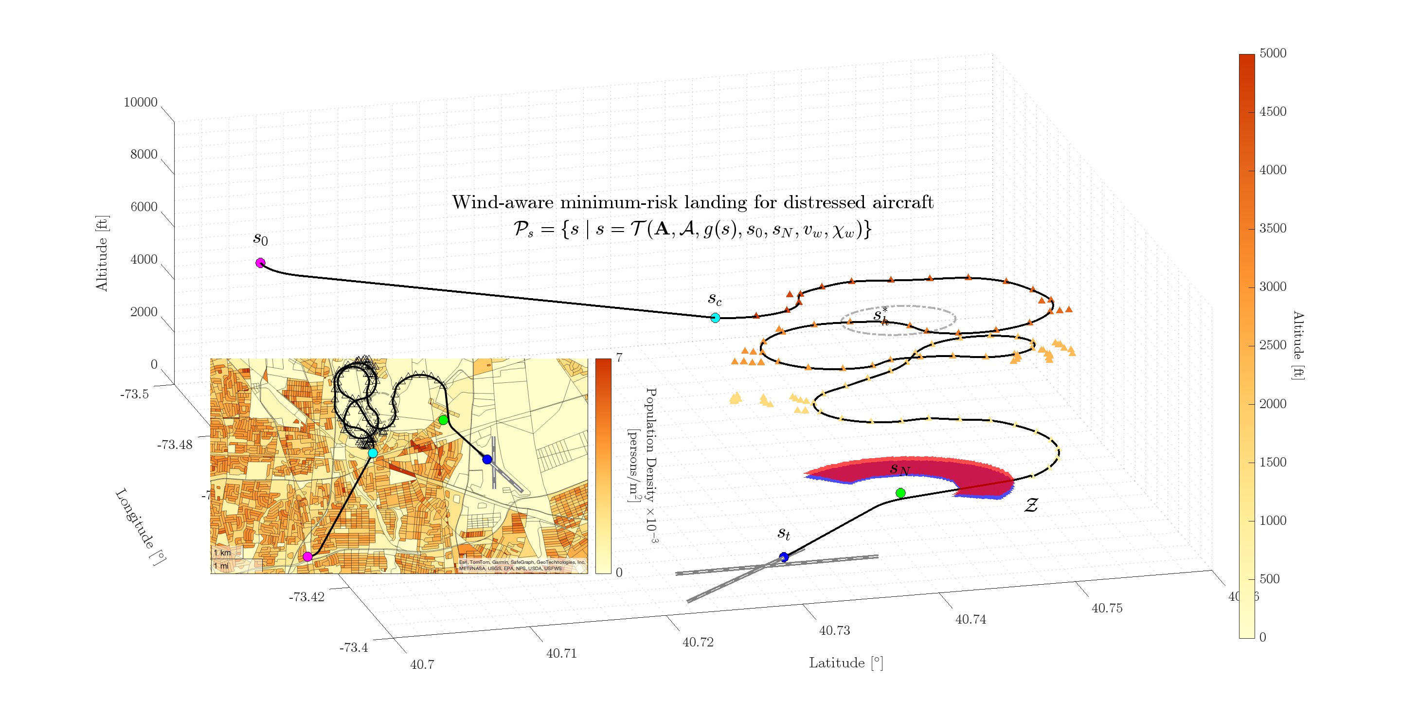
This section presents use cases demonstrating the capabilities of the contingency landing planner under varying altitude conditions and steady wind. Descriptive statistics are also provided on the performance of the proposed method in different initial emergency states over a uniform grid. A populated residential area, Farmingdale, Long Island, NY, is chosen to simulate emergency landing scenarios. Therefore, all use cases and tests share the same goal state: a 1 NM final approach fix at 467 ft mean sea level (MSL) altitude to Runway 14 at Republic Airport (KFRG) in Long Island, New York. Table 2 lists user defined parameters for path planning.
Weight coefficients are used to compute (23) as a function of . A state with a high requires a final approach turn greater than . To mitigate this, state expansion toward regions where the final course change remains below is prioritized. As decreases, is gradually reduced, thereby shifting the cost emphasis toward overflown population and distance to the goal.
6.1. Altitude-Dependent Path Planning
The impact of initial emergency altitude on contingency landing solutions is illustrated in Figure 10, where an emergency scenario is simulated at a randomly selected location within the aircraft footprint, heading to the East, at altitudes of 2500 ft, 6000 ft, and 10000 ft MSL.
At a low emergency onset altitude of 2500 ft MSL, Algorithm 1 directly computes the search-based path and a 3D Dubins path for the final approach to Runway 14 at KFRG, as the initial altitude is below the crossover altitude . The trajectory effectively avoids residential areas by following roads, leveraging available altitude for risk mitigation. This path is computed with as few as 80 explored states, dramatically below the upper bound of the search space size of for this case.
At a high emergency altitude of 10000 ft MSL, altitude dissipation is necessary before approach. A holding pattern is established over a sparsely populated region while maintaining a 0.5 NM no-fly zone around Runway 14 to prevent conflicts with the airport traffic pattern. A 3D Dubins path is then generated from to without considering population risk, as exposure risk at high altitude is minimal due to . The distressed aircraft descends from ft to ft over 8.2 full left-hand holding turns. Despite this descent, excess altitude remains as the aircraft approaches . The gradient-guided search subsequently determines a descent path to that avoids densely populated areas, exploring a total of 72 states. Once the search-based path is generated, a 3D Dubins path is planned from to .
At an initial emergency altitude of 6000 ft, a holding pattern is also identified. However, unlike the 10000 ft case, the landing trajectory deviates from the initial Dubins path upon reaching the crossover altitude at , as the hold inbound cannot be reached above this altitude. From the crossover state , gradient-guided search is initialized. Similar to the example in Figure 4, leads the minimum cost states away from due to the aircraft’s higher altitude relative to the remaining horizontal traversal, causing state expansion away from . This outward expansion is further constrained by the densely populated area in the Northwest of the map, guiding the landing trajectory along the boundary separating low- and high-density regions. As altitude decreases, shifts the minimum-cost states closer to , gradually directing state expansion toward . Compared to the low- and high-altitude cases, the landing path found by the gradient-guided search is significantly longer due to the higher crossover altitude; however, is computed with a total of 110 explored states whereas . As with the previous cases, the final segment is completed with a 3D Dubins path to . The complete 3D contingency landing solution, along with the explored states for the transition case, is shown in Figure 11. The low number of state expansions demonstrates the efficiency of the presented search-based landing planner.
6.2. Contingency Landing Planning Under Steady Wind
Recalling equations (5) and (14), a feasible action depends on wind conditions. A nonzero wind vector alters both the direction and magnitude of the ground speed vector, which in turn affects the required flight path angle to maintain a given airspeed. For path planning, the flight path angle for each segment is selected from a dataset derived from equations (1)-(4), taking into account wind speed and relative direction.
To illustrate the effect of wind on contingency landing planning, two trajectories are compared in Figure 12.
In this emergency scenario, the aircraft begins at 2500 ft MSL with a 10 knot South wind ( kts, ). In windless conditions, the planned trajectory spans 5.41 NM at a constant optimal flight path angle of . However, with a partial tailwind, the feasible flight path angle range becomes shallower with an average optimal flight path angle of , leading to an extended trajectory of 5.53 NM. Steady wind is particularly challenging under headwind conditions which requires a steeper descent. This landing site would not be reachable in case of 10 knots North wind because the feasible flight path angle range would too steeper, resulting in greater altitude loss per unit distance traveled.
6.3. Algorithm Benchmarking on a Uniform Grid
A benchmark study is conducted to evaluate the developed algorithm’s performance in terms of overflown population risk, optimal flight path angle, and computational overhead. Flight time comparison is refrained as it conflicts with the optimal descent. For contingency landing solutions, the implemented framework is compared against 3D and S-turn Dubins paths. To determine the best Dubins-based solution for low-altitude cases, all possible Dubins path types are evaluated and the one that minimizes overflown population risk is selected. Specifically, for lower altitudes, four types of 3D Dubins paths are generated. If additional altitude dissipation is required, S-turn Dubins paths, extending in both directions, are computed and the one with minimum risk is chosen for comparison.
Test scenarios are distributed across a uniform grid with nine coordinates, four altitude levels, and four cardinal directions, totaling 144 unique cases. All initial states are ensured to be reachable from the goal. Algorithm 1 is compared against the minimum-risk Dubins solutions, with results summarized in Table 3, including descriptive statistics on overflown population risk and flight path angle deviation from the optimal.
The search-based method consistently outperforms the Dubins-based approach in minimizing overflown population risk across altitude levels. This is expected as the construction of Dubins paths does not offer explicit risk mitigation.
Meanwhile, the Dubins-based paths adhere strictly to their predefined optimal flight path angles, with deviations close to zero in mid- and high altitude cases. This is because S-turn Dubins paths can precisely achieve the desired altitude loss in case altitude dissipation is needed. In contrast, the search-based method exhibits slight deviations. However, it ensures that these deviations remain within flight envelope and can be further reduced by increasing the discrete search resolution with shorter segment lengths or tighter constraints.
The framework, along with the benchmarking Dubins path solvers, is programmed in C, with the exception of R*-Tree whose source codes are written in C++ [58]. Table 4 provides a detailed runtime analysis benchmarking search-based path planning against the minimum-risk Dubins solutions. For higher altitude scenarios, the total elapsed time for optimal holding point identification and the subsequent Dubins path solution to the hold pattern, labeled as hold planning, are also tabulated. Despite being slower than Dubins solutions as would be anticipated, the developed contingency landing planner exhibits strong potential for real-time implementation. In addition, the separate computation times (44) are provided to highlight its significant contribution to the total computational overhead. As is evident, a high percentage of the total runtime is attributed to the overflown population risk estimation despite an efficient R*-Tree implementation. This overhead could be reduced, albeit with a trade-off in accuracy due to interpolation, by reducing the integration time step or employing data projection methods onto uniform grids.
Table 5 presents the solution availability of Algorithm 2 across 144 test cases for different solver time limits. For initial emergency altitudes of 2500 ft and 5000 ft MSL, the planner provides search-based minimum-risk landing solutions in 67 out of 72 scenarios within the solver time limit of second. At higher altitudes, Algorithm 2 predominantly outputs shortest Dubins solutions due to the hold planning cost, as shown in Table 4. When the solver time limit is increased to seconds, search-based landing solutions are found in 141 out of 144 cases. Only one scenario requires a fallback Dubins solution when seconds is used.
7. Discussion
This paper presented a contingency landing planning framework for an engine-out Cessna 182 model, serving as a surrogate for a distressed AAM aircraft in cruise configuration. However, the proposed approach is adaptable to various emergency scenarios, including but not limited to control surface failures and structural damage by defining the set of feasible actions based on the aircraft’s degraded performance envelope.
To estimate overflown population risk, publicly available population census data is utilized. To improve risk quantification, an interquartile rule for outlier detection was applied. These values were then adjusted to the third quartile population density, ensuring a more representative risk assessment. Alternative population models might be created and updated with real-time data, e.g., from cellular network call data.
In general, the number of explored states in the presented use cases remains low. However, it is observed that when the initial emergency state is located in a densely populated area with a high initial course angle cost, state expansion increases as the algorithm searches for a low-cost trajectory, leading to longer solution times. Additionally, a greater altitude difference between the initial and goal states requires a longer landing path, further increasing state expansion. The gradient-guided search utilizes course angle changes to navigate through narrow low-risk passages. This is not a concern for aircraft with attitude control authority and modern autopilot systems. However, these solutions can only reasonably be shared with air traffic control and other nearby air traffic via datalink to assure coordinated response to separation and collision avoidance.
8. Conclusion
This paper presented a real-time emergency landing planner that combines a novel gradient-guided discrete search with 3D Dubins paths to generate safe and risk-aware landing trajectories for fixed-wing aircraft. To further minimize high-altitude risk, a minimum-risk holding pattern identification algorithm was also introduced. A series of 144 Long Island, New York case studies demonstrated that the presented method significantly reduces risk compared to standard minimum-risk Dubins path solvers. While computationally more demanding, the search-based planner achieved real-time performance, generating minimum-risk landing trajectories within three seconds in 143 out of 144 cases, with a fallback Dubins path returned only once. Future work must consider other air traffic in contingency flight planning solutions to minimize risk associated with disrupting or losing separation with other air traffic. Such solutions will require awareness of commercial and Advanced Air Mobility airspace corridors and reserved geofence volumes for small uncrewed aircraft system traffic. To address this, airspace and air traffic avoidance risks will be captured in contingency landing planning by introducing new cost terms within the gradient-guided search framework.
Author Contributions
Conceptualization, H.E.T. and E.A.; methodology, H.E.T. and E.A; software, H.E.T.; validation, E.A.; formal analysis, H.E.T. and E.A.; investigation, H.E.T. and E.A.; resources, E.A.; data curation, H.E.T. and E.A; writing—original draft preparation, H.E.T. and E.A; writing—review and editing, E.A.; visualization, H.E.T. and E.A.; supervision, E.A.; project administration, E.A.; funding acquisition, E.A. All authors have read and agreed to the published version of the manuscript.
Funding
This research was funded by Langley Research Center grant number 80LARC23DA003.
Data Availability Statement
The original contributions presented in the study are included in the article, further inquiries can be directed to the corresponding author.
Conflicts of Interest
The authors declare no conflicts of interest. The funders had no role in the design of the study; in the collection, analyses, or interpretation of data; in the writing of the manuscript; or in the decision to publish the results.
References
- Bacchini, A.; Cestino, E.; Van Magill, B.; Verstraete, D. Impact of lift propeller drag on the performance of eVTOL lift+ cruise aircraft. Aerospace Science and Technology 2021, 109, 106429. [Google Scholar] [CrossRef]
- Mathur, A.; Atkins, E. Multi-Mode Flight Simulation and Energy-Aware Coverage Path Planning for a Lift+Cruise QuadPlane. Drones 2025, 9. [Google Scholar] [CrossRef]
- Castagno, J.; Atkins, E. Roof Shape Classification from LiDAR and Satellite Image Data Fusion Using Supervised Learning. Sensors 2018, 18. [Google Scholar] [CrossRef]
- Kim, J.; Atkins, E. Airspace Geofencing and Flight Planning for Low-Altitude, Urban, Small Unmanned Aircraft Systems. Applied Sciences 2022, 12. [Google Scholar] [CrossRef]
- Russell, L.; Goubran, R.; Kwamena, F. Emerging Urban Challenge: RPAS/UAVs in Cities. In Proceedings of the 2019 15th International Conference on Distributed Computing in Sensor Systems (DCOSS); 2019; pp. 546–553. [Google Scholar] [CrossRef]
- Dubins, L.E. On Curves of Minimal Length with a Constraint on Average Curvature, and with Prescribed Initial and Terminal Positions and Tangents. American Journal of Mathematics 1957, 79, 497–516. [Google Scholar] [CrossRef]
- Yomchinda, T.; Horn, J.F.; Langelaan, J.W. Modified Dubins parameterization for aircraft emergency trajectory planning. Proceedings of the Institution of Mechanical Engineers, Part G: Journal of Aerospace Engineering 2017, 231, 374–393. [Google Scholar] [CrossRef]
- Chitsaz, H.; LaValle, S.M. Time-optimal paths for a Dubins airplane. In Proceedings of the IEEE CDC; 2007; pp. 2379–2384. [Google Scholar] [CrossRef]
- Ma, D.; Hao, S.; Ma, W.; Zheng, H.; Xu, X. An optimal control-based path planning method for unmanned surface vehicles in complex environments. Ocean Engineering 2022, 245, 110532. [Google Scholar] [CrossRef]
- Bergman, K.; Ljungqvist, O.; Axehill, D. Improved Path Planning by Tightly Combining Lattice-Based Path Planning and Optimal Control. IEEE Transactions on Intelligent Vehicles 2021, 6, 57–66. [Google Scholar] [CrossRef]
- Liu, J.; Han, W.; Liu, C.; Peng, H. A New Method for the Optimal Control Problem of Path Planning for Unmanned Ground Systems. IEEE Access 2018, 6, 33251–33260. [Google Scholar] [CrossRef]
- Zhang, K.; Sprinkle, J.; Sanfelice, R.G. A hybrid model predictive controller for path planning and path following. In Proceedings of the Proceedings of the ACM/IEEE Sixth International Conference on Cyber-Physical Systems, New York, NY, USA, 2015. [CrossRef]
- Shen, C.; Shi, Y.; Buckham, B. Model predictive control for an AUV with dynamic path planning. In Proceedings of the 2015 54th Annual Conference of the Society of Instrument and Control Engineers of Japan (SICE); 2015; pp. 475–480. [Google Scholar] [CrossRef]
- Akametalu, A.K.; Tomlin, C.J.; Chen, M. Reachability-Based Forced Landing System. Journal of Guidance, Control, and Dynamics 2018, 41, 2529–2542. [Google Scholar] [CrossRef]
- Berksetas, D.P. Dynamic Programming and Optimal Control, Volume 1, Third Edition; Athena Scientific, Belmont, 2005.
- Di Donato, P.F.A.; Atkins, E.M. Evaluating Risk to People and Property for Aircraft Emergency Landing Planning. AIAA Journal of Aerospace Information Systems 2017, 14, 259–278. [Google Scholar] [CrossRef]
- Tekaslan, H.E.; Atkins, E.M. Vehicle-to-Vehicle Approach to Assured Aircraft Emergency Road Landings. Journal of Guidance, Control, and Dynamics 2025, 48, 1800–1817. [Google Scholar] [CrossRef]
- Howlett, J.K.; McLain, T.W.; Goodrich, M.A. Learning Real-Time A* Path Planner for Unmanned Air Vehicle Target Sensing. Journal of Aerospace Computing, Information, and Communication 2006, 3, 108–122. [Google Scholar] [CrossRef]
- Qian, Y.; Sheng, K.; Ma, C.; Li, J.; Ding, M.; Hassan, M. Path Planning for the Dynamic UAV-Aided Wireless Systems Using Monte Carlo Tree Search. IEEE Transactions on Vehicular Technology 2022, 71, 6716–6721. [Google Scholar] [CrossRef]
- Chour, K.; Pradeep, P.; Munishkin, A.A.; Kalyanam, K.M. Aerial Vehicle Routing and Scheduling for UAS Traffic Management: A Hybrid Monte Carlo Tree Search Approach. In Proceedings of the 2023 IEEE/AIAA Conference on Digital Avionics Systems; 2023; pp. 1–9. [Google Scholar] [CrossRef]
- Guo, Y.; Liu, X.; Jia, Q.; Liu, X.; Zhang, W. HPO-RRT*: a sampling-based algorithm for UAV real-time path planning in a dynamic environment. Complex & Intelligent Systems 2023, 9, 7133–7153. [Google Scholar] [CrossRef]
- Xu, D.; Qian, H.; Zhang, S. An Improved RRT*-Based Real-Time Path Planning Algorithm for UAV. In Proceedings of the IEEE International Conference on High Performance Computing & Communications; 2021; pp. 883–888. [Google Scholar] [CrossRef]
- Kothari, M.; Postlethwaite, I.; Gu, D.W. Multi-UAV path planning in obstacle rich environments using Rapidly-exploring Random Trees. In Proceedings of the IEEE Conference on Decision and Control; 2009; pp. 3069–3074. [Google Scholar] [CrossRef]
- Sláma, J.; Herynek, J.; Faigl, J. Risk-Aware Emergency Landing Planning for Gliding Aircraft Model in Urban Environments. In Proceedings of the 2023 IEEE/RSJ International Conference on Intelligent Robots and Systems; 2023; pp. 4820–4826. [Google Scholar] [CrossRef]
- Meuleau, N.; Plaunt, C.; Smith, D.; Smith, T. A POMDP for Optimal Motion Planning with Uncertain Dynamics. In Proceedings of the ICAPS-10: POMDP Practitioners Workshop. Citeseer; 2010. [Google Scholar]
- Sharma, P.; Kraske, B.; Kim, J.; Laouar, Z.; Sunberg, Z.; Atkins, E. Risk-Aware Markov Decision Process Contingency Management Autonomy for Uncrewed Aircraft Systems. AIAA Journal of Aerospace Information Systems 2024, 21, 234–248. [Google Scholar] [CrossRef]
- Strube, M.; Sanner, R.; Atkins, E. Dynamic Flight Guidance Recalibration After Actuator Failure. In Proceedings of the AIAA 1st Intelligent Systems Technical Conference; 2004; p. 6255. [Google Scholar]
- Atkins, E.M.; Portillo, I.A.; Strube, M.J. Emergency Flight Planning Applied to Total Loss of Thrust. AIAA Journal of Aircraft 2006, 43, 1205–1216. [Google Scholar] [CrossRef]
- Castagno, J.; Atkins, E. Map-based planning for small unmanned aircraft rooftop landing. In Handbook of Reinforcement Learning and Control; Springer, 2021; pp. 613–646.
- Tekaslan, H.E.; Atkins, E.M. Gradient Guided Search for Aircraft Contingency Landing Planning. In Proceedings of the IEEE International Conference on Robotics and Automation; 2025. [Google Scholar]
- Daniel, K.; Nash, A.; Koenig, S.; Felner, A. Theta*: Any-Angle Path Planning on Grids. Journal of Artifical Intelligence Research 2010, 39, 533–579. [Google Scholar] [CrossRef]
- Beard, R.W.; McLain, T.W. Small Unmanned Aircraft: Theory and Practice; Princeton University Press, 2012.
- Raymer, D. Aircraft Design: A Conceptual Approach, Fifth Edition; American Institute of Aeronautics and Astronautics, Inc., 2012.
- Donato, P. Toward Autonomous Aircraft Emergency Landing Planning. PhD thesis, University of Michigan, Ann Arbor, 2017.
- Napolitano, M.R. Aircraft Dynamics: From Modeling to Simulation; John Wiley, 2011.
- Coombes, M.; Chen, W.H.; Render, P. Reachability Analysis of Landing Sites for Forced Landing of a UAS. Journal of Intelligent & Robotic Systems 2013, 73, 635–653. [Google Scholar] [CrossRef]
- Matthew Coombes, W.H.C.; Render, P. Landing Site Reachability in a Forced Landing of Unmanned Aircraft in Wind. AIAA Journal of Aircraft 2017, 54, 1415–1427. [Google Scholar] [CrossRef]
- Arslantaş, Y.E.; Oehlschlägel, T.; Sagliano, M. Safe landing area determination for a Moon lander by reachability analysis. Acta Astronautica 2016, 128, 607–615. [Google Scholar] [CrossRef]
- Kirchner, M.R.; Ball, E.; Hoffler, J.; Gaublomme, D. Reachability as a Unifying Framework for Computing Helicopter Safe Operating Conditions and Autonomous Emergency Landing. IFAC-PapersOnLine 2020, 53, 9282–9287. [Google Scholar] [CrossRef]
- Chen, M.; Tomlin, C.J. Hamilton–Jacobi Reachability: Some Recent Theoretical Advances and Applications in Unmanned Airspace Management. Annual Review of Control, Robotics, and Autonomous Systems 2018, 1, 333–358. [Google Scholar] [CrossRef]
- Di Donato, P.F.A.; Atkins, E.M. Optimizing Steady Turns for Gliding Trajectories. AIAA Journal of Guidance, Control, and Dynamics 2016, 39, 2627–2637. [Google Scholar] [CrossRef]
- Shanmugavel, M.; Tsourdos, A.; White, B.; Zbikowski, R. 3D Dubins Sets Based Coordinated Path Planning for Swarm of UAVs. In Proceedings of the AIAA Guidance, Navigation, and Control Conference; 2006. [Google Scholar]
- Shanmugavel, M.; Tsourdos, A.; White, B.; Żbikowski, R. Cooperative path planning of multiple UAVs using Dubins paths with clothoid arcs. Control Engineering Practice 2010, 18, 1084–1092. [Google Scholar] [CrossRef]
- Fallast, A.; Messnarz, B. Automated trajectory generation and airport selection for an emergency landing procedure of a CS23 aircraft. CEAS Aeronautical Journal 2017, 8, 481–492. [Google Scholar] [CrossRef]
- Di Donato, P.F.A.; Balachandran, S.; McDonough, K.; Atkins, E.; Kolmanovsky, I. Envelope-Aware Flight Management for Loss of Control Prevention Given Rudder Jam. AIAA Journal of Guidance, Control, and Dynamics 2017, 40, 1027–1041. [Google Scholar] [CrossRef]
- Bacon, B.; Gregory, I. General Equations of Motion for a Damaged Asymmetric Aircraft. In Proceedings of the AIAA Atmospheric Flight Mechanics Conference and Exhibit; 2012. [Google Scholar] [CrossRef]
- Lampton, A.; Valasek, J. Prediction of Icing Effects on the Lateral/Directional Stability and Control of Light Airplanes. In Proceedings of the AIAA Atmospheric Flight Mechanics Conference and Exhibit; 2012. [Google Scholar] [CrossRef]
- Imagery, N.; (NIMA), M.A. Department of Defense World Geodetic System 1984, Its Definition and Relationships With Local Geodetic Systems. Technical Report TR MD, 2000.
- US. Census Bureau. RACE. U.S. Census Bureau. Accessed on 6 November 2023.
- Rana, I.K. An Introduction to Measure and Integration, Second Edition; American Mathematical Society, 2002.
- Chae, S.B. Lebesgue Integration, Second Edition; Springer, 1995.
- Beckmann, N.; Kriegel, H.P.; Schneider, R.; Seeger, B. The R*-tree: an efficient and robust access method for points and rectangles. SIGMOD Rec. 1990, 19. [Google Scholar] [CrossRef]
- Johnson, S.G. The NLopt nonlinear-optimization package. https://github.com/stevengj/nlopt, 2007.
- Bandi, S.; Thalmann, D. Space discretization for efficient human navigation. Computer Graphics Forum 1998, 17, 195–206. [Google Scholar] [CrossRef]
- Henrich, D.; Wurll, C.; Worn, H. Online path planning with optimal C-space discretization. In Proceedings of the IEEE International Conference on Intelligent Robots and Systems, Vol. 3; 1998; pp. 1479–1484. [Google Scholar] [CrossRef]
- Russell, S.; Norvig, P. Artificial Intelligence: A Modern Approach, 3 ed.; Prentice Hall Series, Pearson, 2010.
- Hart, P.E.; Nilsson, N.J.; Raphael, B. A Formal Basis for the Heuristic Determination of Minimum Cost Paths. IEEE Transactions on Systems Science and Cybernetics 1968, 4, 100–107. [Google Scholar] [CrossRef]
- Libspatialindex Contributors. libspatialindex: A General Framework for Spatial Indexing, 2025. "Accessed: Feb 2025".
Figure 1.
Fundamental forces acting in the aircraft longitudinal plane.
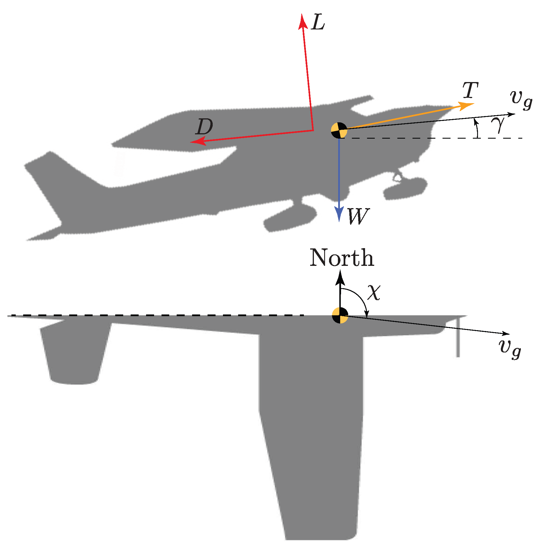
Figure 2.
Contingency landing paths for low-altitude, high-altitude, and transition cases. A circular holding pattern is used for high-altitude cases.
Figure 2.
Contingency landing paths for low-altitude, high-altitude, and transition cases. A circular holding pattern is used for high-altitude cases.
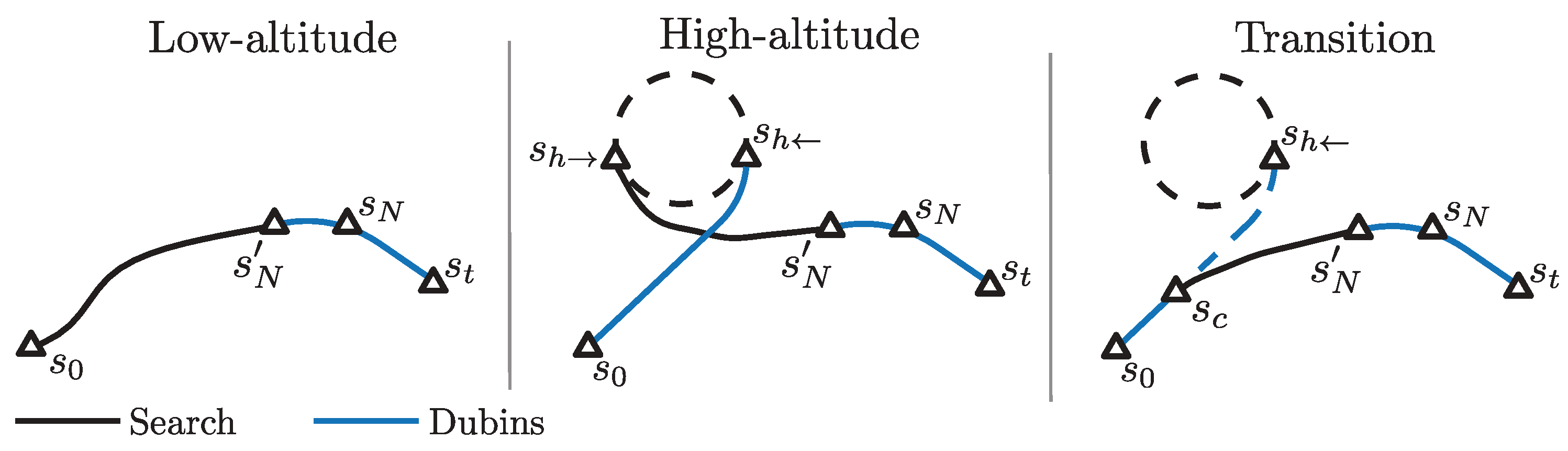
Figure 3.
Planar geometry of sequential turns.
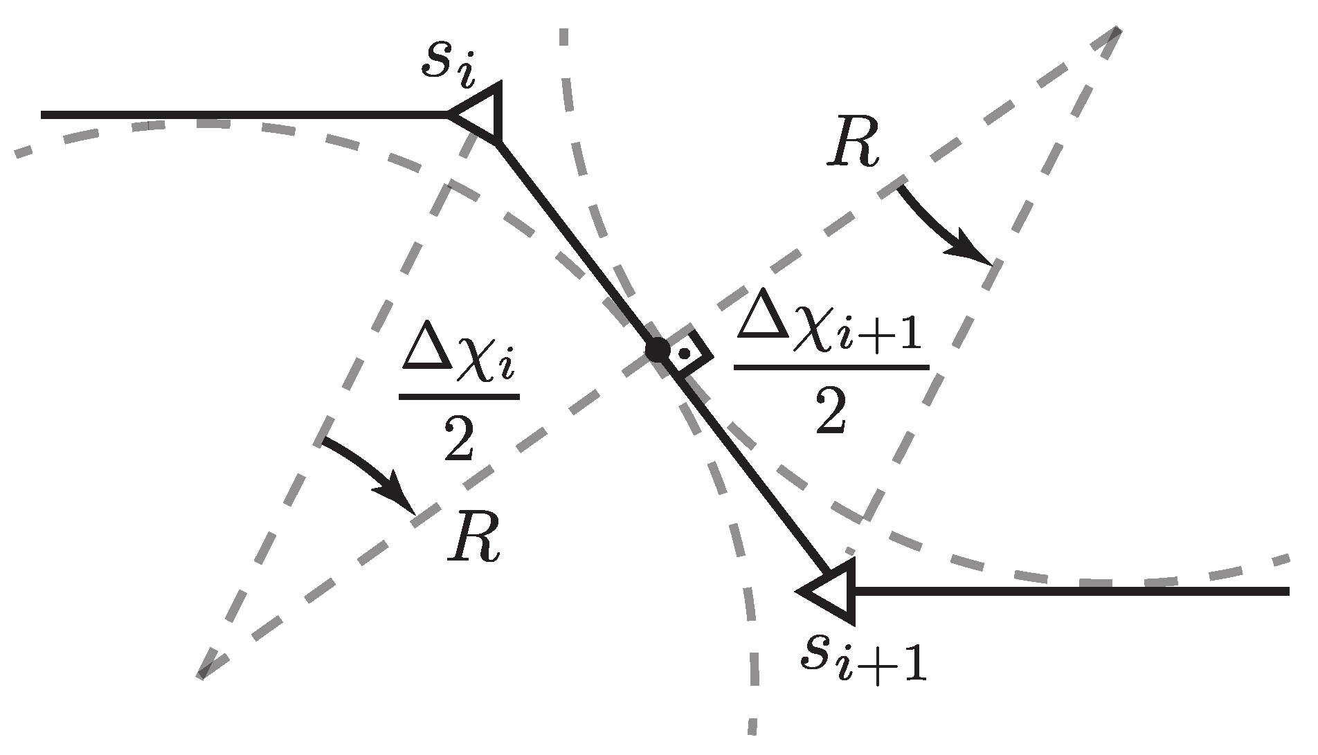
Figure 4.
An evolution of with a vector field around the goal state. Red arrows show course angle.
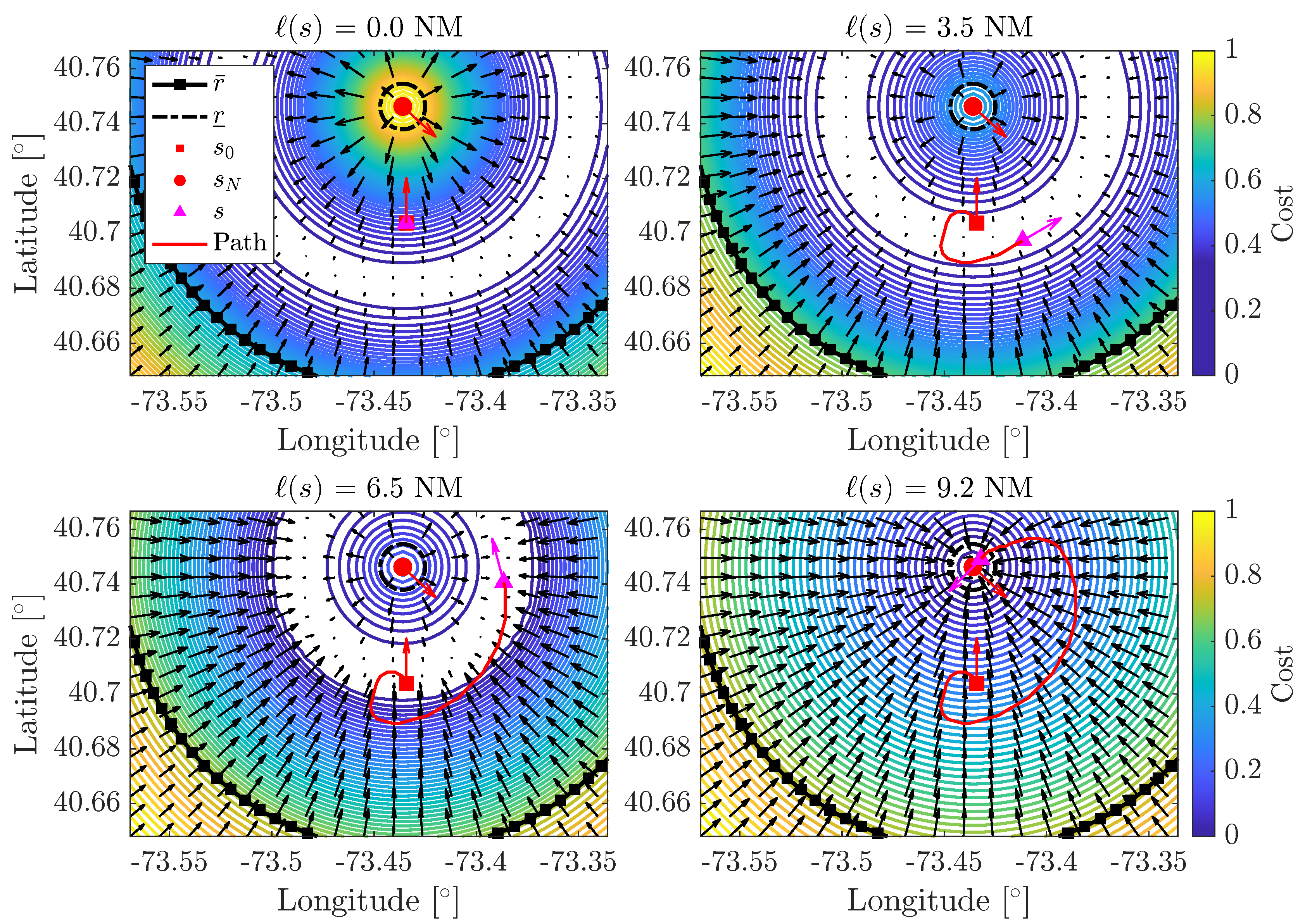
Figure 5.
A map of the course angle cost. The black dashed line illustrates the state bisecting plane. Red arrows show course angle.
Figure 5.
A map of the course angle cost. The black dashed line illustrates the state bisecting plane. Red arrows show course angle.
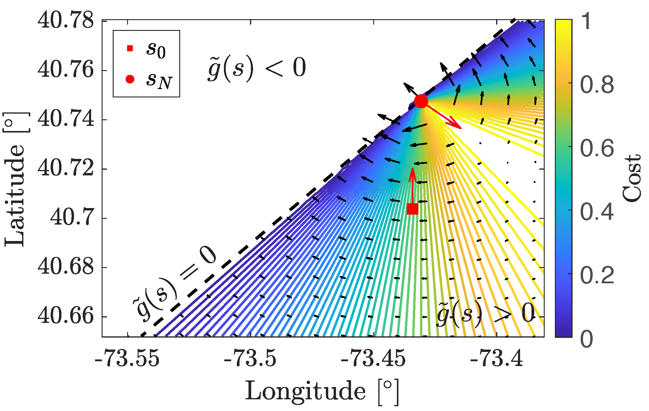
Figure 6.
Evolution of the total distance and course angle costs with a vector field around a goal state. Red arrows show course angle.
Figure 6.
Evolution of the total distance and course angle costs with a vector field around a goal state. Red arrows show course angle.
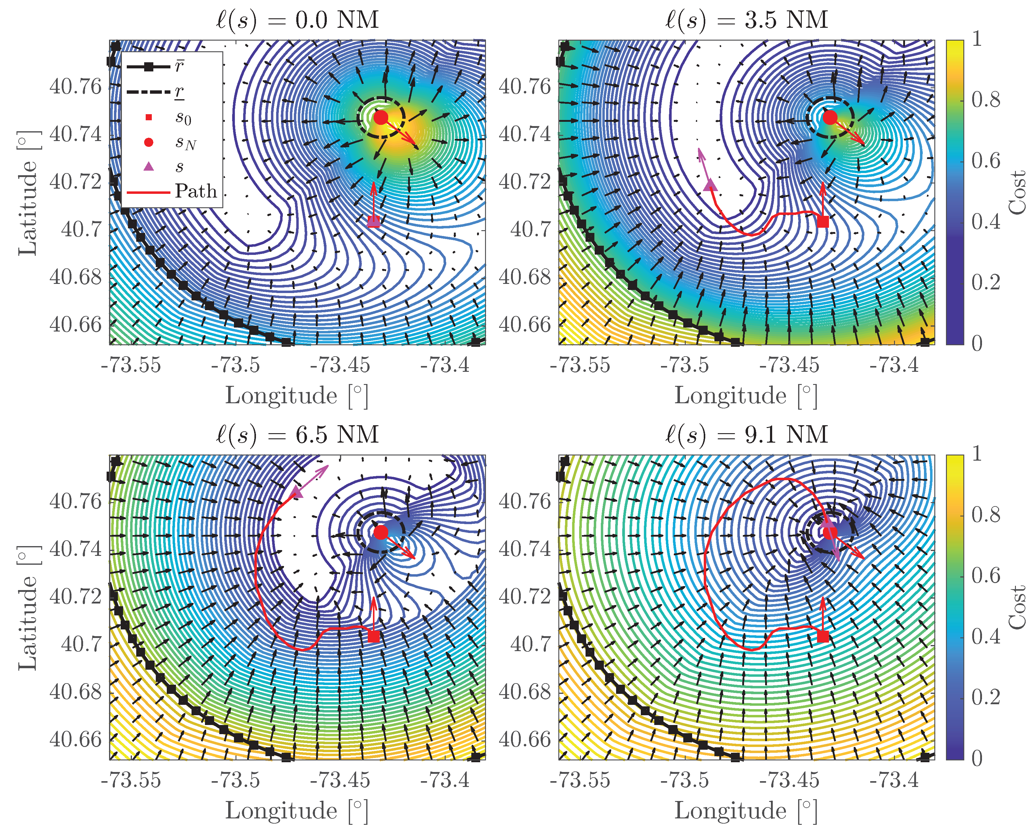
Figure 7.
A representative solution identification set.
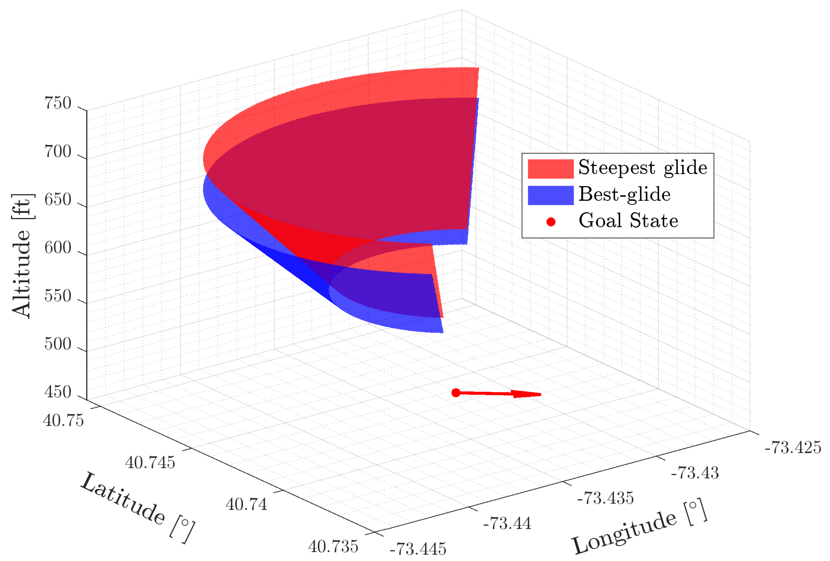
Figure 8.
Hold inbound state determination.
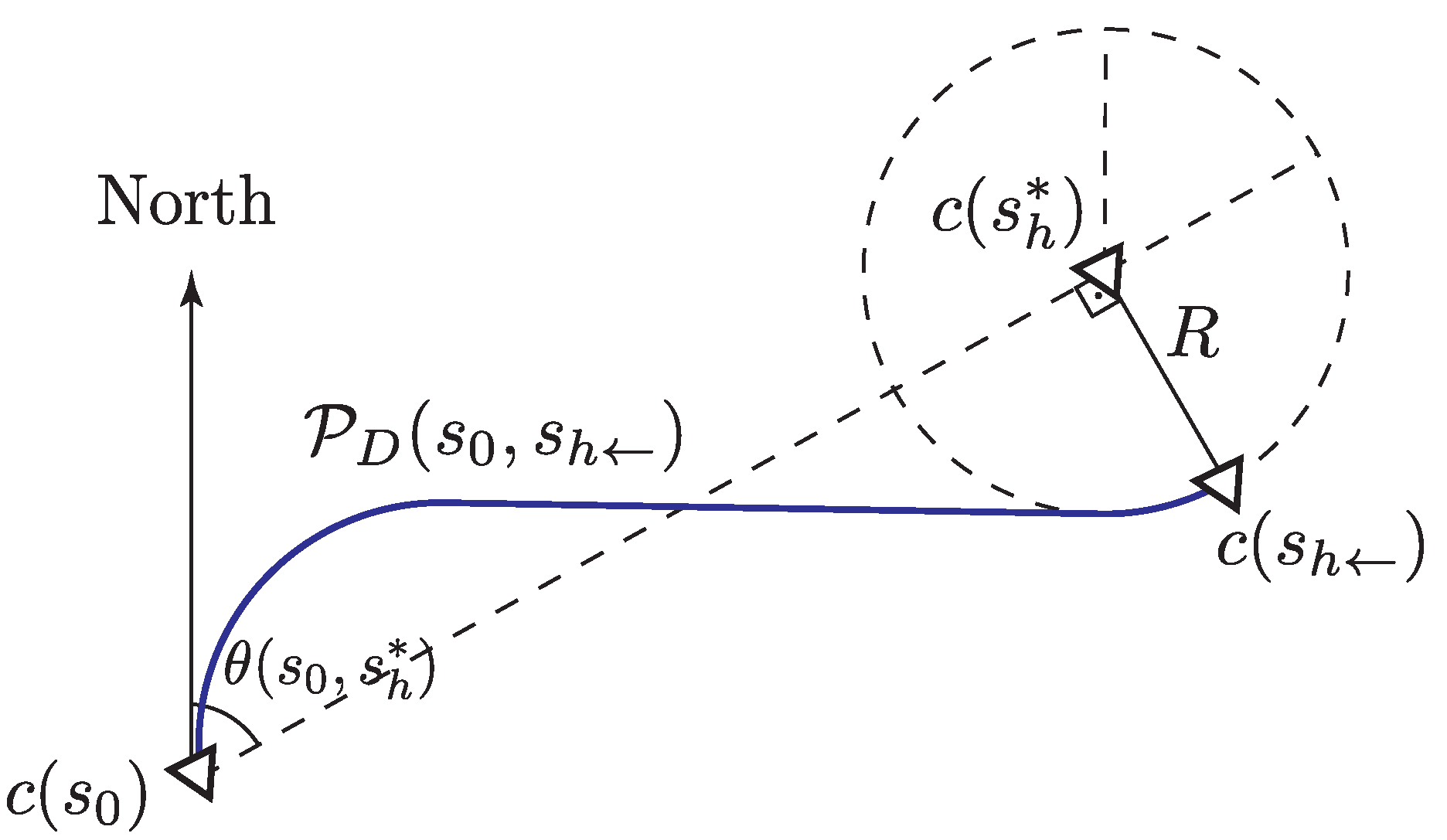
Figure 9.
An illustration of a discrete search space in 3D.
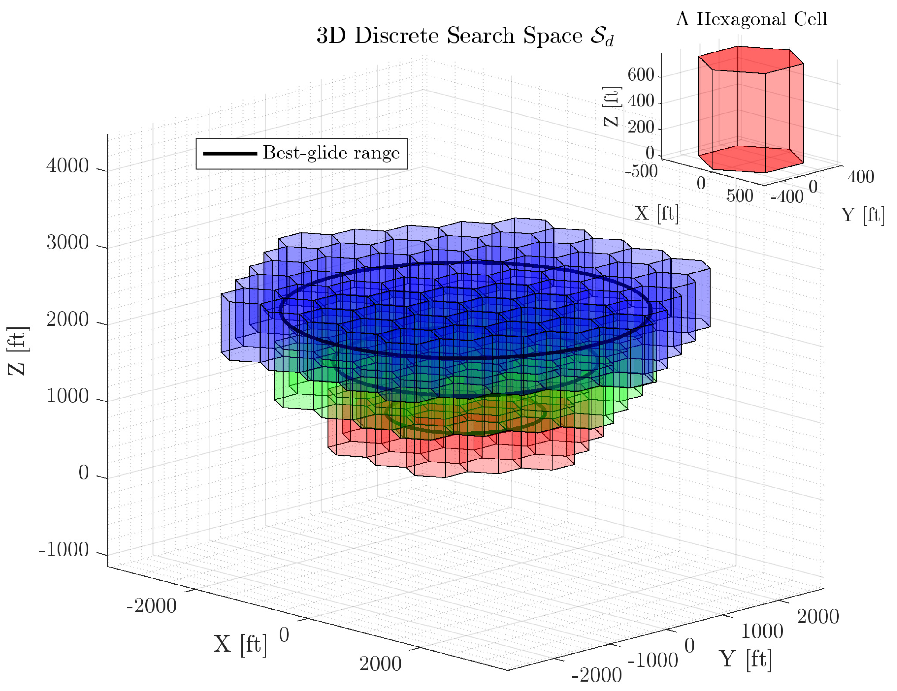
Figure 10.
Contingency landing solutions for varying initial altitudes.
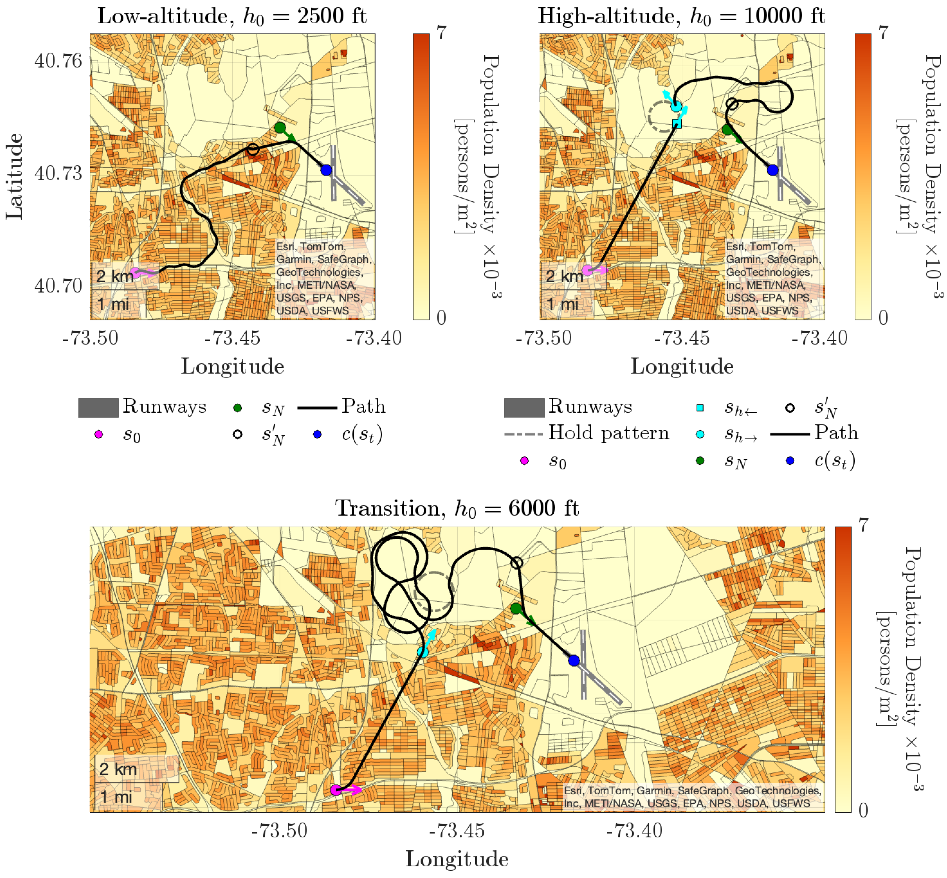
Figure 11.
The 3D contingency landing trajectory and explored state coordinates for the transition case, initially at 6000 ft MSL.
Figure 11.
The 3D contingency landing trajectory and explored state coordinates for the transition case, initially at 6000 ft MSL.
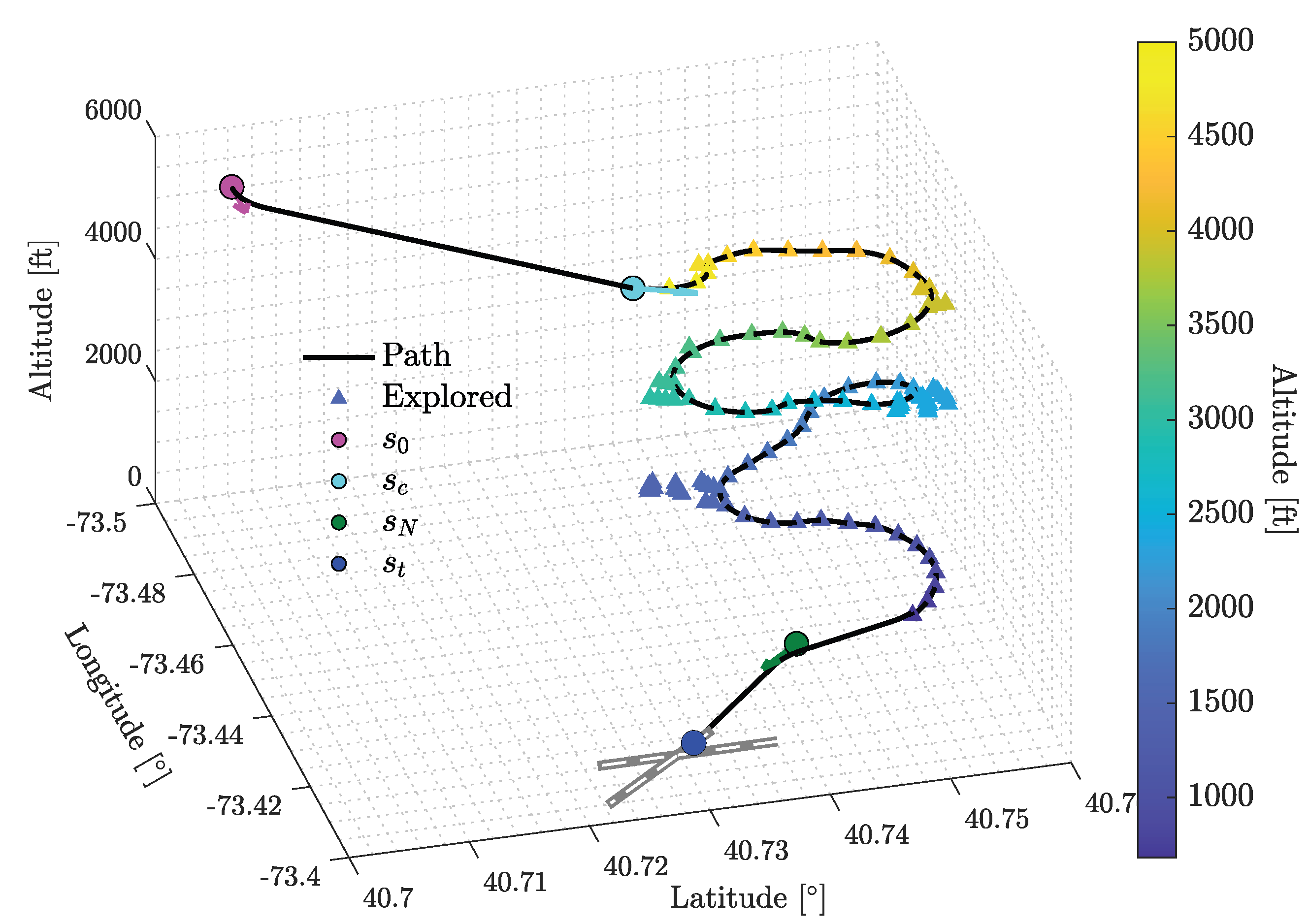
Figure 12.
The impact of tailwind in the contingency landing solution.
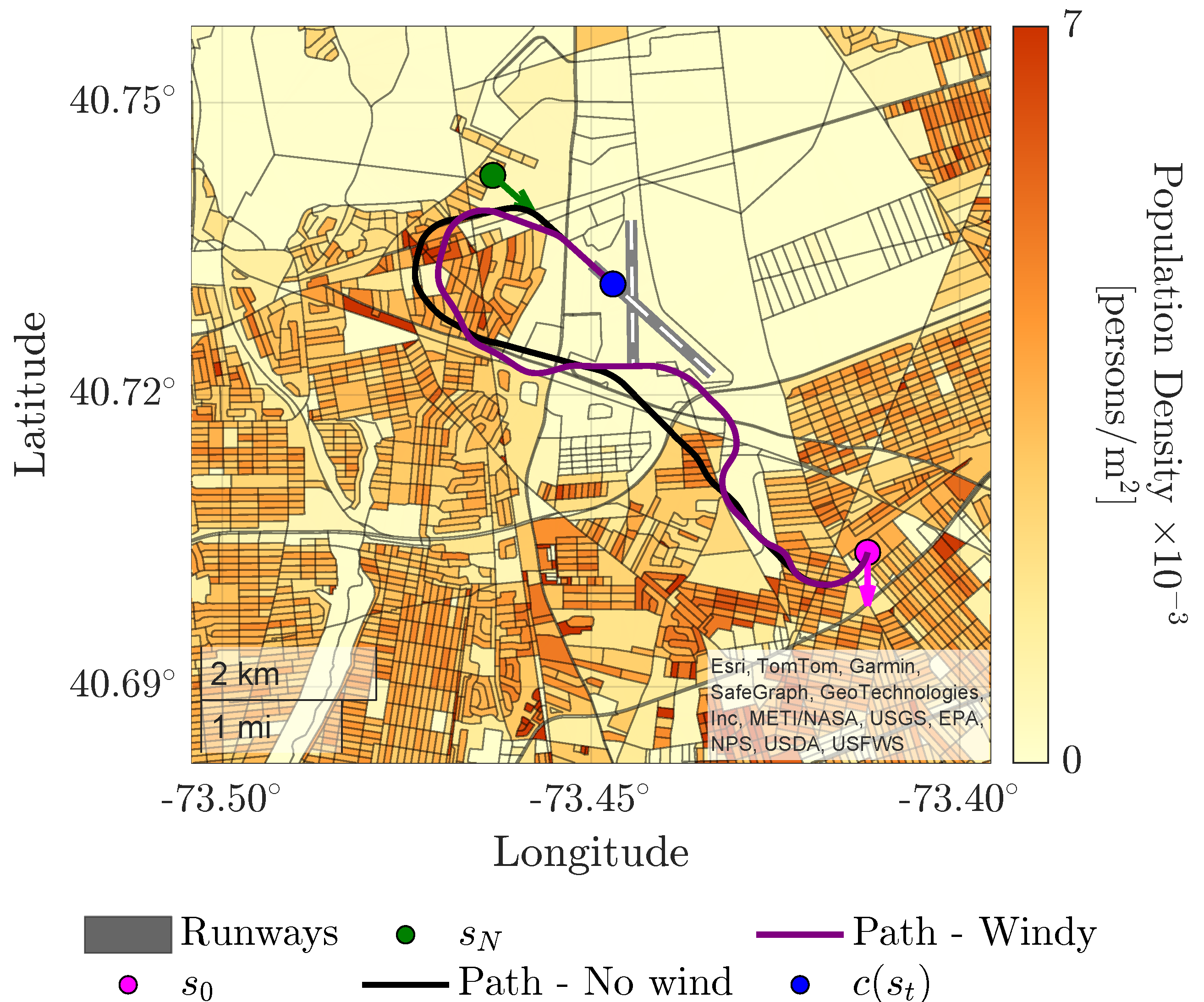

Table 1.
Upper bounds of discrete search space size for the Cessna 182 experiencing loss of thrust.
| [ft] | for Different Circumradii in ft | ||
|---|---|---|---|
| 500 | 1000 | 1500 | |
| 500 | |||
| 2500 | |||
| 5000 | |||
Table 2.
Parameters for altitude-dependent path planning.
| Parameter | Value | Unit |
|---|---|---|
| R | 1500 | ft |
| 5000 | ft | |
| °C | ||
| 2000, 0.1 | ft, - | |
| 0.5 | NM | |
| 1500, 3000 | ft, ft | |
| 1000 | ft | |
| 1500 | ft | |
| 5 | °C | |
| Weight coefficients as a function of | ||
| Condition on | Cost Weights | |
Table 3.
Risk and gliding constraint comparison of the gradient-guided search and the minimum-risk 3D Dubins solutions.
Table 3.
Risk and gliding constraint comparison of the gradient-guided search and the minimum-risk 3D Dubins solutions.
| [ft] | Method | Population Risks | Deviation [°C] | ||||||
|---|---|---|---|---|---|---|---|---|---|
| Min. | Max. | Median | Max. | ||||||
| 2500 | Search | 0.0006 | 0.2157 | 0.0221 | 0.0418 | 0.0451 | 0.30 | -0.06 | 0.09 |
| Dubins | 0.0028 | 0.2048 | 0.0620 | 0.0667 | 0.0575 | 0.27 | -0.02 | 0.06 | |
| 5000 | Search | 0.0021 | 0.1183 | 0.0085 | 0.0206 | 0.0260 | 0.23 | -0.07 | 0.04 |
| Dubins | 0.0132 | 0.1987 | 0.0704 | 0.0843 | 0.0574 | 0.00 | 0.00 | 0.00 | |
| 6000 | Search | 0.0010 | 0.0136 | 0.0038 | 0.0046 | 0.0035 | 0.29 | -0.09 | 0.08 |
| Dubins | 0.0022 | 0.1317 | 0.0267 | 0.0358 | 0.0373 | 0.00 | 0.00 | 0.00 | |
| 10000 | Search | 0.0014 | 0.0101 | 0.0045 | 0.0047 | 0.0023 | 0.27 | -0.05 | 0.07 |
| Dubins | 0.0021 | 0.0388 | 0.0068 | 0.0106 | 0.0090 | 0.00 | 0.00 | 0.00 | |
Table 4.
Runtime comparison of the gradient-guided search and the minimum-risk 3D Dubins solutions in C-language.
Table 4.
Runtime comparison of the gradient-guided search and the minimum-risk 3D Dubins solutions in C-language.
| [ft] | Method | Total Runtime [ms] | Risk () Computation Runtime [ms] | ||||||||
|---|---|---|---|---|---|---|---|---|---|---|---|
| Min. | Max. | Median | Min. | Max. | Median | ||||||
| 2500 | Search | 27.0 | 764.5 | 92.2 | 135.1 | 128.8 | 26.0 | 671.6 | 89.6 | 129.3 | 115.2 |
| Dubins | 8.2 | 121.4 | 67.9 | 63.5 | 28.6 | 8.1 | 68.3 | 34.3 | 35.7 | 18.1 | |
| 5000 | Search | 133.0 | 6897.0 | 441.4 | 723.1 | 1140.3 | 130.3 | 4963.5 | 432.4 | 646.3 | 820.0 |
| Dubins | 99.7 | 221.2 | 167.7 | 162.0 | 31.6 | 89.2 | 210.9 | 158.9 | 153.1 | 31.1 | |
| 6000 | Hold Planning | 963.9 | 1120.8 | 987.7 | 1003.4 | 41.0 | 24.0 | 66.4 | 49.2 | 48.0 | 10.4 |
| Search | 76.5 | 1947.3 | 180.5 | 314.5 | 358.7 | 74.8 | 1893.8 | 175.1 | 305.9 | 349.1 | |
| Dubins | 59.9 | 226.2 | 94.8 | 114.0 | 47.6 | 42.9 | 218.8 | 82.0 | 100.6 | 51.8 | |
| 10000 | Hold Planning | 976.5 | 1127.2 | 1033.8 | 1034.9 | 31.9 | 24.5 | 69.1 | 50.2 | 49.2 | 11.2 |
| Search | 37.8 | 510.8 | 175.3 | 197.1 | 116.1 | 36.8 | 495.5 | 168.7 | 190.2 | 112.3 | |
| Dubins | 46.0 | 105.9 | 73.0 | 75.6 | 16.0 | 15.2 | 81.8 | 54.7 | 53.7 | 15.4 | |
| All experiments are conducted using a single core of Apple M2 chip (3.49 GHz). | |||||||||||
Table 5.
Algorithm 2 solution availability for different time limits.
| [s] | [ft] | Number of solutions | ||||
|---|---|---|---|---|---|---|
| 2500 | 5000 | 6000 | 10000 | Search-based | Fallback Dubins () | |
| 1 | 36 | 31 | 0 | 1 | 68 | 76 |
| 2 | 36 | 35 | 34 | 36 | 141 | 3 |
| 3 | 36 | 35 | 36 | 36 | 143 | 1 |
Short Biography of Authors
 |
H. Emre Tekaslan is a Ph.D. candidate at the Kevin T. Crofton Aerospace and Ocean Engineering Department at Virginia Tech. He holds a B.S. degree in Aeronautical Engineering and an M.S. degree in Aeronautical and Astronautical Engineering from Istanbul Technical University (2019, 2022). During his M.S. studies, he pursued research in multidisciplinary low-boom supersonic aircraft design optimization and scientific machine learning. In addition to his research activities, he volunteered in a NATO Science and Technology Organization Applied Vehicle Technology Panel. H. Emre’s current research area focuses on aircraft contingency landing management. In recognition of his work, he has been awarded the Boeing Scholarship and the Pratt Fellowship. He is a reviewer for the AIAA Journal of Aerospace Information Systems and AIAA Journal of Aircraft. He is also a student glider pilot. |
 |
Ella M. Atkins is Fred D. Durham Professor and Head of the Kevin T. Crofton Aerospace and Ocean Engineering Department at Virginia Tech. She was previously a Professor in the University of Michigan’s Aerospace Engineering and Robotics Departments. Dr. Atkins holds B.S. and M.S. degrees in Aeronautics and Astronautics from MIT (1988, 1990) and M.S. and Ph.D. degrees in Computer Science and Engineering from the University of Michigan (1995, 1999). She is an AIAA Fellow and private pilot. She has authored over 250 refereed journal and conference papers. Dr. Atkins pursues research in AI-enabled autonomy and control to support resilience and contingency management in crewed and uncrewed Aerospace applications with focus on Advanced Air Mobility and Uncrewed Aircraft Systems (UAS). She is Editor-in-Chief of the AIAA Journal of Aerospace Information Systems (JAIS). |
Disclaimer/Publisher’s Note: The statements, opinions and data contained in all publications are solely those of the individual author(s) and contributor(s) and not of MDPI and/or the editor(s). MDPI and/or the editor(s) disclaim responsibility for any injury to people or property resulting from any ideas, methods, instructions or products referred to in the content. |
© 2025 by the authors. Licensee MDPI, Basel, Switzerland. This article is an open access article distributed under the terms and conditions of the Creative Commons Attribution (CC BY) license (http://creativecommons.org/licenses/by/4.0/).
Copyright: This open access article is published under a Creative Commons CC BY 4.0 license, which permit the free download, distribution, and reuse, provided that the author and preprint are cited in any reuse.


