Submitted:
06 August 2025
Posted:
07 August 2025
You are already at the latest version
Abstract
The objective of this study is to explore the applicability of area cartograms for the visualization of sustainable development indicator components, utilizing earth observation (EO) data. The analysis focuses on selected Sustainable Development Goals (SDG 11 and SDG 13) and specific targets related to green urban areas and air quality (targets 13.2, 11.6, and 11.7). A comprehensive review of the relevant literature indicates that area cartograms are employed only sporadically in the context of SDGs monitoring, particularly at lower levels of territorial division (i.e., municipalities and counties). To address this gap, a series of thematic maps − including choropleth maps and irregular area cartograms − were developed. These visualizations are based on EO-derived datasets and supplemented with statistical information obtained from the Local Data Bank of the Central Statistical Office of Poland. The analysis demonstrates that area cartograms provide an effective means of visualizing spatial disparities in variables such as urban green space availability and air pollution at the municipal and county levels. These visualizations enhance the interpretability of complex indicator structures and support more nuanced assessments of progress toward selected Sustainable Development Goals, especially in spatially detailed analytical frameworks.
Keywords:
area cartogram
; cartographic method
; SGDs
; earth observation data
; visual analytics
; cartography
1. Introduction
Monitoring the achievement of the Sustainable Development Goals (SDGs) is an important topic that can be assisted by using indicators elaborated based on Earth Observation (EO) data. The United Nations (UN) Sustainable Development Goals are global development targets adopted in 2015. All countries have agreed to work towards achieving them by 2030 [1]. The Sustainable Development Goals (SDGs) form a closely linked set of priorities, where progress in one area often affects outcomes in others. Reaching these goals requires finding a practical balance between environmental protection, economic growth, and social well-being. Their implementation depends not only on political will but also on the involvement of institutions, local governments, and civil society. To monitor progress, the UN Secretary-General releases an annual report prepared in collaboration with the UN system, using data collected by national statistical offices and regional partners [2]. These reports contain information on the realization of particular SDG goals, targets, and indicators, part of which is presented on maps. Statistics Poland (SP) is responsible for presenting the implementation of the SDGs in Poland. On the Institution's website, it is possible to find information about 250 global indicators with data for Poland for monitoring the Sustainable Development Goals (SDGs).
The study presents indicators related to SDG11 (Goal 11 – Sustainable cities & communities), and SDG13 (Goal 13 – Climate action). As a preliminary step, the following targets and indicators were selected for analysis:
- Target 11.6: Reduce the environmental impacts of cities (Indicator 11.6.2 – Annual mean levels of fine particulate matter);
- Target 11.7: Provide access to safe and inclusive green and public spaces (Indicator 11.7.1 – Average share of the built-up area of cities that is open space for public use for all);
- Target 13.2: Integrate climate change measures into national policies, strategies, and planning (Indicator 13.2.2 – Total greenhouse gas emissions per year).
Air pollution remains a major challenge in urban areas. Elevated concentrations of particulate matter (PM), nitrogen oxides (NO₂), tropospheric ozone (O₃), sulfur dioxide (SO₂) are known to negatively impact human health and quality of life in affected regions. These pollutants also contribute to the degradation of biodiversity and the disruption of ecosystem functions. According to the World Health Organization (WHO) and the European Environment Agency (EEA), long-term exposure to air pollution is associated with reduced life expectancy and increased rates of premature mortality. These concerns are reflected in the Sustainable Development Goals, particularly Target 11.6, which aims to reduce the per capita environmental impact of cities, with a focus on air quality and waste management. The related Indicator 11.6.2 measures the annual mean levels of fine particulate matter (PM2.5 and PM10) in urban areas, weighted by population. In the context of air quality monitoring (SDG 11.6.2 and 13.2.2, Figure 1.), advanced earth observation (EO) techniques are employed, integrating multi-temporal Copernicus Sentinel-5P satellite data with deep learning models. This approach monitors pollutants such as NO₂, SO₂, tropospheric ozone, CO, CH₄, CH₂O, and particulate matter (PM2.5, PM10) [3]. These products are supplemented with meteorological data and ground-based measurements. Deep learning models enable precise classification of pollution levels, combining satellite and in situ data for improved accuracy [4]. For studies conducted in Poland, satellite-derived products are validated using national monitoring networks (e.g., the Chief Inspectorate of Environmental Protection), ensuring their reliability [5]. Within this framework, detailed spatial and temporal pollution maps can be developed using GIS and geoinformation platforms. Such maps support urban management, public health planning, and policy-making, particularly in areas with limited ground-based monitoring, contributing to effective and scalable air quality assessment aligned with SDGs targets.
Green areas, addressed in SDG Indicator 11.7.1, are particularly important in densely populated cities, where they contribute to local climate regulation and provide accessible spaces for recreation. In addition to their environmental functions, green spaces support public health and social interaction, which can strengthen neighborhood ties. As a result, they play a measurable role in enhancing the quality of life in urban environments [7,8,9]. Recognizing their significance, there is a growing need to develop comprehensive and up-to-date systems to monitor and assess green areas, enabling informed decision-making for sustainable urban development [10,11,12]. The Sustainable Development Goals (SDGs) focus on creating sustainable cities and communities, emphasising the importance of green areas, e.g., SDG Target 11.7: “By 2030, provide universal access to safe, inclusive and accessible, green and public spaces in particular for women and children, older persons and persons with disabilities” as an integral component of urban planning and development. Urban green space, such as parks and gardens, play a crucial role in enhancing the well-being of urban residents, promoting environmental health, and contributing to overall urban resilience [13,14,15,16]. In the literature, numerous studies are available that utilize remote sensing to assess the availability of green areas within the framework of the Sustainable Development Goals in Poland [17,18]. Within the GAUSS project [6], (Figure 2), a green space assessment system was developed by integrating Sentinel-2 satellite data, vegetation products from the Copernicus Land Monitoring Service, and in situ information. To ensure accurate and reliable validation, the database of topographic objects (BDOT10k) was utilized, enabling detailed characterization of green spaces across Poland. By combining these diverse data sources, the developed service allows end-users to effectively monitor green spaces through the generation of annual statistics accompanied by statistical maps of Poland at the municipal level.
2. Related Studies
An analysis of 120 selected publications showed that 19 different cartographic methods were applied to visualize the SDG indicators 11.6.2, 11.7.1, and 13.2.2. (Figure 3). Only in five cases dasymetric solutions [19,20,21,22,23] and in two cases – a cartogram [24,25] were employed. Almost all cases were static solutions. Only in one case a comparison of multiple time states [26] was employed to visualize the greenhouse gas emissions in China in 2000-2011 period. Only one interactive solution was used [27] to present the average air quality map of the greater Cleveland area.
It should be emphasized that the use of cartographic methods differs significantly in the case of visualization of the three analyzed indices. For the 11.6.2 indicator visualization, the shaded isolines method is used in more than 43% of cases e.g.: [28,29,30,31,32,33,34,35,36,37,38]. Two cases of its combined use with bars have been identified [39,40] and only one case of combination with choropleth map [41]. Relatively often (28%), a grid with a different size of the basic field was used as a cartographic presentation method for the visualization of the 11.6.2 indicator [42,43,44,45,46,47,48,49]. Sometimes it was limited to the area of communication routes (e.g.: [49]). There have been cases of it being combined with choro-pleth maps (4%, e.g.: [48]), as well as with shaded isolines (2%, e.g.: [44]). Much less frequent (4%) were the cases of using quantitative signatures (e.g.: [51,52]). One case of combined use of quantitative signatures with grid and choropleth method was identified [53]. Relatively rare were the cases of using the choropleth maps (e.g.: [54]), line choropleth maps (e.g.: [55]), cross choropleth maps (e.g.: [56]), as well as the combined use of choropleth maps with ordinary signatures (e.g.: [57]). Only 2 % of the solutions involved the use of isolines (e.g.: [58]) and vector maps (e.g.: [59]). In most cases, it is used to present the location of green areas in cities.
In the case of the 11.7.1 indicator, the most frequently used solution is the choro-chromatic method, used in 38% of publications (e.g.: [60,61,62,63,64,65,66] ). 16% are applications of the choropleth method, with units related to city districts (e.g.: [67,68,69,70,71,72]. Isochrone (e.g.: [73,74,75,76]) and grid (e.g.: [77,78,79,80,81]) applications constitute 8% each. Quantitative point signatures are used in 6% (e.g.: [82,83])., while buffer (e.g.: [84,85]), qualitative point signatures (e.g.: [86,87]) and dasymetric choropleth maps (e.g.: [19]) – only 4% each. The least frequently used methods for 11.7.1 indicators are: linear choropleth maps ([88]) proportional symbols (e.g.: [89]), shaded isolines (e.g.: [90]) and radius maps (e.g.: [91]).
The relatively smallest diversity of methods used for visualization occurs in the case of indicator 13.2.2. The most commonly used are choropleth map (e.g.: [92,93,94,95]) and grid (e.g.: [96,97]) − 35% each. In addition, the following methods are used: shaded isolines [98], structural diagrams [99], dasymetric method [100] and cartogram [101]. Depending on the aggregation of available data, indicators are visualized in relation to different spatial units.
In the case of 11.6.2 SDG indicator 50% of maps were elaborated using the point data, which were mostly employed to build the isoline maps (43 %). The other 7 % point data (7 %) allowed to use quantitative point signatures. 28 % of maps employed different grid cells like a spatial units. In 2% of cases the data was related to the NUTS 3. The same percentage was found in the case of city districts and functional areas of cities. In the 4,35 % of cases the spatial units were dense grid of streets. The same percentage was used in attempts to link the index value with land cover elements in cities.
In the case of 11.7.1 SDG indicator 38% of maps were elaborated using the land use data concerning the cities. In 24% of cases, the spatial reference for this indicator was the division units. 10% of them were city districts and 4% − city functional areas. In 4% of cases, the analysis covered areas within functional areas, while in 6% of cases, the analysis covered areas bounded by streets. Grid with different basic fields was used in 10% of the maps presenting the 11.7.1 indicator.
In the case of 13.2.2 SDG indicator 45% maps were elaborated using remote sensing data, concerning the entire Earth. In 25% of cases the data was related to countries (NUTS 0), in 20% to NUTS 2 and only in 10% to NUTS 3. In 5% the 13.2.2 SDGs indicators were related to the global land use data.
It should be emphasized that in the case of analyzed maps of 11.6.2, 11.7.1 13.2.2 SDGs indicators there was no case of referring data from the EO registration to the smallest units of administrative division at the area of whole country. This solution was used in the case of the article [6].
A critical examination of the relevant literature indicates that cartograms have been employed only infrequently in the representation of sustainable development indicators at the municipal and county levels, highlighting a notable gap in spatial visualization practices at finer administrative scales.
3. Materials and Methods
This study examines area cartograms employed for monitoring changes in Sustainable Development Goal (SDG) indicators using earth observation (EO) data. The objective is to assess the respective advantages and limitations of this approach in the context of tracking progress toward the SDGs. The prepared maps focus on two key themes aligned with SDG 11 and SDG 13: urban green spaces and air pollution (PM2.5, PM10, NOx). Both the spatial extent and condition of green areas, as well as the concentrations of selected air pollutants, were derived from Earth observation data. The applied methodology have been described in Introduction.
3.1. Study Area
As part of the study, statistical maps were generated to illustrate data for Poland at various administrative levels: at the commune (gmina) level (Figure 4 left) and the county (powiat) level (Figure 4 right). Poland is a country in Central Europe, covering an area of approximately 312,696 square kilometers. Its administrative structure is organized into three main tiers: 16 voivodeships (provinces), 380 counties (poviats), and 2,477 communes (gminas). This territorial division reflects a decentralized governance model aimed at improving administrative efficiency at regional and local levels.
3.2. Topic
3.2.1. Air Polution
Particulate Matter with a diameter ≤ 2.5 µm (PM2.5) refers to fine particulate matter with an aerodynamic diameter of 2.5 micrometers or smaller [102]. These particles are small enough to penetrate deep into the respiratory tract and reach the alveoli, posing significant health risks. PM2.5 originates from both natural sources, such as wildfires and dust storms, and anthropogenic (human-made) activities, including vehicle emissions, industrial processes, and residential combustion. Secondary PM2.5 can also form in the atmosphere through chemical reactions involving precursors such as sulfur dioxide (SO₂), nitrogen oxides (NOₓ), and volatile organic compounds (VOCs). Due to their small size and chemical composition, PM2.5 particles are a major concern for air quality and public health monitoring.
Particulate Matter with a diameter ≤ 10 µm (PM10) refers to a mixture of solid particles and liquid droplets suspended in the air. These particles are small enough to be inhaled and can penetrate the respiratory system, potentially causing adverse health effects. PM10 originates from various sources, including road traffic, industrial processes, and natural sources such as dust or pollen. It is commonly used as an indicator of general air quality, especially in urban environments.
Nitrogen oxides (NOx) is a collective term for nitrogen monoxide (NO) and nitrogen dioxide (NO₂), two major air pollutants produced primarily during high-temperature combustion processes, such as those in vehicle engines and power plants. NOx plays a significant role in atmospheric chemical reactions, contributing to the formation of ground-level ozone, smog, and secondary particulate matter. These compounds are harmful to human health, particularly affecting the respiratory system, and also contribute to environmental problems such as acid rain and eutrophication. In air quality assessments, NOx is a key indicator of combustion-related pollution, especially in urban and industrial areas.
3.2.2. Green Areas
The maps presented in this publication were prepared using definitions of green areas derived from Nature Protection criteria. According to the Polish Act [103] green areas including technical infrastructure and buildings functionally associated with them, covered with vegetation, located in the village of dense buildings or cities, used for the aesthetic, recreational, therapeutic or shielding purposes, in particular parks, lawns, promenades, boulevards, botanical and zoological gardens, children's playgrounds, historic garden, cemeteries, green areas located near roads in the build-up areas, squares, historic fortifications, buildings, landfill sites, airports, railway stations and industrial buildings. The application of this definition enables the classification of green areas in relation to SDG 11.
3.3. Data Sources
3.3.1. Air Polution
The Copernicus Atmosphere Monitoring Service (CAMS) reanalysis is the most recent global reanalysis dataset of atmospheric composition (AC) developed under the European Union’s Copernicus Earth observation programme. It provides three-dimensional, time-consistent fields of key atmospheric constituents, including aerosols, reactive gases, and greenhouse gases. The dataset benefits from methodological advancements and operational experience gained through the preceding Monitoring Atmospheric Composition and Climate (MACC) reanalysis and the CAMS interim reanalysis. The current dataset spans the period from 2003 to December 2023. CAMS reanalysis data are provided at a horizontal resolution of approximately 80 km, with both sub-daily and monthly temporal resolution, and cover a wide range of atmospheric variables [104].
To obtain yearly averages of air pollutants (PM2.5, PM10, NOx), datasets from CAMS and GUGiK were utilized. The process involved converting hourly pollution data from NetCDF to TIFF format, cropping it to Poland’s borders, and calculating monthly averages for each pixel. These monthly images were then resampled, stacked, and used to compute average pollutant concentrations for local administrative units (LAUs). Finally, yearly averages were calculated from monthly data for each pollutant, combined into a single dataset, and converted into a vector file for analysis and mapping.
3.3.2. Green Areas
The study produced maps focusing on two fundamental attributes of urban green spaces: their distribution and health status. The extent of green areas was delineated using Sentinel-2 data and products from the GAUSS project [6], with a spatial resolution of 10 meters. To achieve a more precise delineation of green areas at the commune level, in addition to satellite data, detailed vector boundaries from BDOT10k (Topographic Objects Database at a 1:10,000 scale) were used. Sentinel-2 products were also utilized to assess the condition of urban green spaces.
Values of the widely used Normalized Difference Vegetation Index (NDVI) were derived from Sentinel-2 data to enable comparison with a novel vegetation index based on High-Resolution Vegetation Phenology and Productivity (HR-VPP) data. Subsequently, the data on the extent and condition of green areas were aggregated to the commune level (LAUs). Depending on the chosen cartographic presentation method (choropleth maps, or area cartograms) additional statistical data from the Local Data Bank (Central Statistical Office) were incorporated. These supplementary datasets included demographic information, such as population by age groups at the commune level, and vehicle counts at the county level.
3.4. Map Production
3.4.1. Colour Legend
An integral component of the map development process was the creation of legends for the choropleth maps illustrating air pollution. Reference ranges for pollutant particle concentrations and their corresponding map colors were adopted from the literature (Table 1.). These color scales were subsequently adjusted to better reflect the dataset. In the later stages of map preparation, additional subdivisions were introduced within the scales while maintaining the original color scheme—for example, the 'good air quality' category was refined by incorporating lighter and darker shades of green.
3.4.2. Choropleth Maps
All choropleth maps were created using QGIS Desktop, version 3.38.0. The underlying base map was the 2020 administrative division of Poland, delineated at the county (powiat) or municipality (gmina) level. For all choropleth maps, the 'natural breaks' (Jenks) classification method was applied, meaning that class intervals were optimized based on the frequency distribution of the data in order to minimize within-class variance and maximize between-class variance.
3.4.3. Area Cartograms
The cartogram is a map on which one feature – distance (distance cartograms) or area (area cartograms) is distorted proportionally to the value of a given phenomenon [105]. This presentation addresses selected area cartograms, placing special emphasis on automatically generated rectangular cartograms. Various software tools can be used to generate contiguous area cartograms [106]. These may include dedicated software for designing cartograms, plugins or toolboxes for GIS applications, or scripts written in programming languages—particularly in R. A review of selected software tools that support the automated generation of contiguous area cartograms is presented in Table 2.
The irregular Gastner-Newman cartograms in this publication were produced using the QGIS Desktop plugin cartogram3 version 3.1.5. The resulting maps were generated over two iterations for municipalities (gminy) and five iterations for counties (poviaty), with a maximum mean error in the anamorphosis process not exceeding 15%.
4. Results
4.1. Air Polution
The initial set of maps focuses on air pollution issues related to Sustainable Development Goals (SDGs) 11.6 and 13.2. In the first phase, three choropleth maps were produced (Figure 5), illustrating the spatial distribution of PM2.5, PM10, and NOx concentrations, respectively in LAUs in 2020. A uniform color scale was applied throughout, with green hues indicating the lowest levels of air pollution. The analysis of these maps indicates that, in 2020, the overall air quality in Poland was relatively good. However, elevated pollutant concentrations were recorded in major urban areas (e.g., Warsaw, Łódź), within the Upper Silesian Industrial Region (particularly in the case of PM2.5), and along key transportation corridors (especially NOx, notably the belt extending from Warsaw and Łódź toward the Upper Silesian region). According to the spatial patterns presented on the maps, the areas with the lowest air pollution concentrations are located in northern Poland—especially along the Baltic Sea and in proximity to the Kaliningrad and Lithuanian borders—and in the mountainous regions of the south, such as the Bieszczady and Tatras.
The second step involved producing area cartograms to depict PM2.5 and PM10 concentrations within Polish municipalities in 2020 (Figure 6). The area of each municipality on the cartograms is scaled proportionally to its population. This approach was chosen because population size directly relates to emissions, as residential sources constitute the main contributors to both PM2.5 and PM10 pollution.
It can be observed that on the cartograms, larger municipal areas generally correspond to lighter shades of green or yellow. The use of cartograms distinctly highlights municipalities with large populations but small geographic areas and their associated pollution levels. On cartograms, major cities become distinctly visible, including Szczecin, the Tricity metropolitan area (Gdańsk), Poznań, Łódź, Warsaw, Wrocław, the Upper Silesian Industrial Region, and Kraków, roughly arranged from northwest to southeast. In contrast, these areas were less clearly represented in the previous standard choropleth maps (Figure 6), where cities like Szczecin, the Tricity, and parts of the Upper Silesian conurbation appeared less prominent.
In the NOx concentration cartogram, the territorial division of Poland into counties (poviaty) was used, with the area of each unit scaled according to the number of vehicles registered in that county in 2020 (Figure 7). Applying an area cartogram in this context produced a notably informative outcome: counties with the largest visual representation—reflecting the highest number of registered vehicles—are consistently shaded in the lightest green, corresponding to the highest NOx concentrations. This spatial pattern is not as easily discernible in the standard choropleth map presented on the left side of Figure 7. By using the area cartogram, NOx concentrations in the Tricity area became clearly discernible − something that was challenging on the choropleth map owing to the small size of the constituent urban counties.
Nevertheless, it is important to acknowledge that the application of area cartograms can result in considerable spatial distortions. This is especially evident in counties with large territorial extent but relatively few registered vehicles, which can complicate the interpretation of data in regions such as Eastern Poland.
4.2. Green Areas
The choropleth map (Figure 8) and area cartograms (Figure 8 and Figure 9) were generated for green areas to illustrate both their coverage and overall condition. Figure 8 presents the extent of green areas using a choropleth map, as well as both the extent and condition of green areas using a cartogram. In the choropleth map, increasingly intense shades of green indicate a higher proportion of urban green space relative to the total municipal area. In the cartogram, the intensity of the green shade corresponds to the condition of green spaces − the stronger the hue, the better the ecological state.
It is evident that in certain municipalities, including Warsaw and the Tricity, green areas represent a substantial proportion of the total municipal territory; however, their ecological condition ranges from moderate to poor. Such nuanced information cannot be as effectively discerned from the choropleth map alone.
In relation to Target 11.7 — 'Provide access to safe and inclusive green and public spaces' — a critical consideration is the assessment of accessibility for specific demographic groups, particularly children and the elderly. Figure 9 presents a set of cartograms illustrating both the excent and ecological condition of green areas in correlation with the number of children (aged 0–14) residing in each municipality. Findings indicate that in municipalities with relatively large child populations, the ecological condition of green spaces is not necessarily high. The use of area cartograms enhances the interpretive capacity of spatial analyses by simultaneously representing accessibility and environmental quality. This approach underscores the critical role of green space quality in supporting the health, development, and well-being of younger demographic groups.
4. Discussion and Conclusion
Despite the growing importance of spatially disaggregated data in sustainability assessments, cartographic research has seldom addressed the visualization of SDG indicators at detailed territorial scales. The cartographic methods most frequently applied in the context of the Sustainable Development Goals (SDGs) are choropleth and grid maps. These visualizations, however, are typically limited to national or broad regional levels of analysis.
The synthesis of existing academic research (part 2 Related Studies), demonstrates that the use of area cartograms in the representation of Sustainable Development Goals (SDGs) remains exceedingly limited, especially in studies employing earth observation data. Moreover, where such techniques have been applied, they have largely been restricted to aggregated territorial units, with little attention given to subnational levels such as counties or municipalities. A notable exception is the publication Mapping for a Sustainable World [112] where Section 3.8 briefly explores the potential of area cartograms for visualizing SDG-related data at the national scale.
The analysis of existing literature, combined with the cartographic outputs developed in this study, highlights the practical value of using area cartograms to visualize Sustainable Development Goal (SDG) indicators. This method is particularly useful in representing urban areas, which are often visually minimized in traditional cartographic techniques such as choropleth maps due to their small geographic size. This issue is especially relevant in the Polish administrative context, where rural municipalities typically cover much larger areas than urban units, including cities with county status.
Despite these advantages, certain limitations of area cartograms must be acknowledged. Irregular or highly distorted cartograms may impede the legibility and spatial recognition of individual administrative units, particularly for end users without prior familiarity with the geographic configuration of the study area. Such distortions can pose challenges to interpretability and reduce the communicative effectiveness of the map.
The results of this study indicate several strategic directions for advancing the application of cartograms in the spatial visualization of SDG-related phenomena, particularly in contexts involving continuous Earth Observation (EO) data:
- applying area cartograms to represent spatial units with highly variable population sizes at lower administrative levels (e.g., municipalities, counties). This technique enhances the visibility and interpretability of densely populated urban areas, which are often spatially limited but demographically significant;
- integrating Earth Observation data into the construction of area cartograms, which enriches the thematic content of the maps and enables more frequent and dynamic monitoring of urban environments compared to conventionally collected statistical datasets. EO-based inputs offer higher temporal resolution and spatial consistency, supporting timely assessments of sustainability indicators;
- combining area cartograms with other cartographic techniques, such as choropleth maps, proportional symbols, or qualitative and quantitative point signatures. Such hybrid visualizations provide a more comprehensive representation of SDG-related issues by simultaneously conveying multiple dimensions of the data.
Author Contributions
Conceptualization, A.M.; methodology, A.M. and D.D.; validation, A.M.; formal analysis, A.M.; data curation, A.M. and D.D.; writing—original draft preparation, A.M. and D.D.; writing—review and editing, A.M., D.D.; visualization, A.M.; supervision, A.M. All authors have read and agreed to the published version of the manuscript.
Funding
This research received no external funding.
Conflicts of Interest
The authors declare no conflicts of interest.
Abbreviations
The following abbreviations are used in this manuscript:
| BDOT10k | Topographic Objects Database |
| CAMS | Copernicus Atmosphere Monitoring Service |
| EEA | European Environment Agency |
| EO | Earth observation |
| GIS | Geographic information system |
| GUGiK | Head Office of Geodesy and Cartography in Poland |
| HR-VPP | High-Resolution Vegetation Phenology and Productivity |
| LAU | Local administrative unit |
| NDVI | Normalized Difference Vegetation Index |
| NO2 | Nitrogen oxides |
| NUTS | Nomenclature of Territorial Units for Statistics |
| O3 | Tropospheric ozone |
| PM | Particulate matter |
| SGDs | Sustainable Development Goals |
| SO2 | Sulphur dioxides |
| SP | Statistics Poland |
| UN | United Nations |
| WHO | World Health Organization |
References
- UN General Assembly, 2015. Transforming our world: the 2030 Agenda for Sustainable Development, A/RES/70/1, 21 October 2015. https://www.refworld.org/legal/resolution/unga/2015/en/111816.
- UN DESA, 2024. The Sustainable Development Goals Report 2024 – June 2024. New York, USA: UN DESA. © UN DESA. https://unstats.un.org/sdgs/report/2024/.
- Lamsal, L. N., Martin, R. V., Parrington, M., Krotkov, N. A., van Donkelaar, A., Celarier, E. A., ... & Sioris, C. E. (2021). A Senti-nel-5P TROPOMI derived nitrogen dioxide (NO₂) product for air quality monitoring. Atmospheric Measurement Techniques, 14(6), 2607–2633.
- Kassomenos, P., Bais, A., Dandou, A., & Katsafados, P. (2018). Machine learning models for predicting urban air quality using satellite and ground-based observations. Atmospheric Environment, 189, 54–66. [CrossRef]
- Buczyńska, A., Szpak, M., & Sobik-Szołtysek, J., 2020. Satellite-based assessment of air quality over Poland using Sentinel-5P data. Environmental Pollution, 263, 114462. [CrossRef]
- Panek-Chwastyk, E., Dąbrowska-Zielińska, K., Markowska, A., Kluczek, M., Pieniążek, M., 2024. Advanced utilization of satellite and governmental data for determining the coverage and condition of green areas in Poland: An experimental statistics supporting the Statistics Poland. International Journal of Applied Earth Observation and Geoinformation, Vol. 130, 103883. [CrossRef]
- Czekajlo, A., Coops, N.C., Wulder, M.A., Hermosilla, T., Lu, Y., White, J.C., Van Den Bosch, M., 2020. The urban greenness score: A satellite-based metric for multi-decadal characterization of urban land dynamics. Int. J. Appl. Earth Obs. Geoinf. 93, 102210 . [CrossRef]
- Jabbar, M., Yusoff, M.M., Shafie, A., 2022. Assessing the role of urban green spaces for human well-being: A systematic review. GeoJournal 87, 4405–4423. [CrossRef]
- Liu, K., Li, X., Wang, S., Gao, X., 2022. Assessing the effects of urban green landscape on urban thermal environment dynamic in a semiarid city by integrated use of airborne data, satellite imagery and land surface model. Int. J. Appl. Earth Obs. Geoinf. 107, 102674 . [CrossRef]
- Cheng, Y., Wang, W., Ren, Z., Zhao, Y., Liao, Y., Ge, Y., Wang, J., He, J., Gu, Y., Wang, Y., Zhang, W., Zhang, C. (2023) ‘Multi-scale feature fusion and transformer network for urban green space segmentation from high-resolution remote sensing images’. Int. J. Appl. Earth Observ. Geoinf. 124, 103514. [CrossRef]
- Wang, X., Meng, Q., Zhang, L., Hu, D., 2021. Evaluation of urban green space in terms of thermal environmental benefits using geographical detector analysis. Int. J. Appl. Earth Obs. Geoinf. 105, 102610 . [CrossRef]
- Wu, W.-B., Ma, J., Meadows, M.E., Banzhaf, E., Huang, T.-Y., Liu, Y.-F., Zhao, B., 2021. Spatio-temporal changes in urban green space in 107 Chinese cities (1990–2019): The role of economic drivers and policy. Int. J. Appl. Earth Obs. Geoinf. 103, 102525 . [CrossRef]
- Gelan, E., Girma, Y., 2022. Urban green infrastructure accessibility for the achievement of SDG 11 in rapidly urbanizing cities of Ethiopia. GeoJournal 87, 2883–2902. [CrossRef]
- Giuliani, G., Petri, E., Interwies, E., Vysna, V., Guigoz, Y., Ray, N., Dickie, I., 2021. Modelling accessibility to urban green areas using open earth observations data: A novel approach to support the urban SDG in four European Cities. Remote Sens. (Basel) 13, 422. [CrossRef]
- Lorenzo-Sáez, E., Lerma-Arce, V., Coll-Aliaga, E., Oliver-Villanueva, J.-V., 2021. Contribution of green urban areas to the achievement of SDGs. Case study in Valencia (Spain). Ecol. Ind. 131, 108246 . [CrossRef]
- Savchenko, A.B., Borodina, T.L., 2020. Green and digital economy for sustainable development of urban areas. Reg. Res. Russ. 10, 583–592. [CrossRef]
- Krzyżaniak, M., Świerk, D., Szczepańska, M., Urbański, P., 2018. Changes in the area of urban green space in cities of western Poland. Bull. Geogr. Soc.-Econ. Ser. 39, 65–77. [CrossRef]
- Wysmułek, J., Hełdak, M., Kucher, A., 2020. The analysis of green areas’ accessibility in comparison with statistical data in Poland. IJERPH 17, 4492. [CrossRef]
- Gavrilidis, A. A., Popa, A-M., Onose, D. A., Gradinaru, S. R., 2022, Planning small for winning big: Small urban green space distribution patterns in an expanding city, Urban Forestry & Urban Greening 78 (2022) 127787. [CrossRef]
- Guo, H., 2022, Big Earth Data in Support of the Sustainable Development Goals (2022)—The Belt and Road, Sustainable Develop-ment Goals Series, Springer Nature. [CrossRef]
- Ruiz-Apilánez, B. Ormaetxea, E., Aguado-Moralejo, I., 2023, Urban Green Infrastructure Accessibility: Investigating Environmental Justice in a European and Global Green Capital. Land 2023, 12, 1534. [CrossRef]
- Stessens, P., Khan, A. Z., Marijke Huysmans, M., Canters, F., 2017, Analysing urban green space accessibility and quality: A GIS-based model as spatial decision support for urban ecosystem services in Brussels, Ecosystem Services 28 (2017) 328–340. [CrossRef]
- Vukmirovic, M., Gavrilovic, S., Stojanovic, D., 2019, The Improvement of the Comfort of Public Spaces as a Local Initiative in Coping with Climate Change, Sustainability 2019, 11, 6546; [CrossRef]
- Carbon Dioxide Emissions 2015 - Worldmapper, 2.07.2025, 13:02.
- Hennig, B., 2012, Emissions of Greenhouse Gases. https://www.viewsoftheworld.net/.
- Tian, Y., Zhu, Q., Lai K., Y.H. Lun, V., 2014, Analysis of greenhouse gas emissions of freight transport sector in China, Journal of Transport Geography 40 (2014) 43–52. [CrossRef]
- Interactive 2024 Average Air Quality Map of the Greater Cleveland Area - Mold and Air Duct Pros, May 28, 2024.
- Bertazzon, S., Shahid, R., 2019, Schools, Air Pollution, and Active Transportation: An Exploratory Spatial Analysis of Calgary, Canada, Int. J. Environ. Res. Public Health 2017, 14, 834; [CrossRef]
- Daramola, S.O, Makinde, E.O., 2024, Modeling air pollution around major dumpsites in Lagos State using geospatial methods with solutions, Environmental Challenges 16 (2024) 100969. [CrossRef]
- Duan, J., Li, Y., Li, S., Yang, Y., Li, F., Li, Y., Wang, J., Deng, P., Wu, J., Wang, W., Meng, Ch., Miao, R., Chen, Z., Zou, B., Yuan, H., Cai, J., Lu, Y., 2022, Association of Long-term Ambient Fine Particulate Matter (PM2.5) and Incident CKD: Prospective Cohort Study in China, AJKD Vol 80, Iss 5, November 2022. [CrossRef]
- Habermann, M., Billger, M., Haeger-Eugensson, M., 2015, Land use regression as method to model air pollution. Previous results for Gothenburg/Sweden, Procedia Engineering 115 ( 2015 ) 21 – 28. [CrossRef]
- Lisberg Jensen, E., Karin Westerberg, K., Malmqvist, E., Oudin, A., 2020, Through Internet and Friends: Translation of Air Pollu-tion Research in Malmö Municipality, Sweden, Int. J. Environ. Res. Public Health 2020, 17, 4214; [CrossRef]
- Liu, X., Bertazzon, S., 2016, Fine Scale Spatio-Temporal Modelling of Urban Air Pollution, J.A. Miller et al. (Eds.): GIScience 2016, LNCS 9927, pp. 210–224, 2016. [CrossRef]
- Mijling, B., 2020, High-resolution mapping of urban air quality with heterogeneous observations: a new methodology and its application to Amsterdam, Atmos. Meas. Tech., 13, 4601–4617, 2020. [CrossRef]
- Obanya, H.E., Amaeze,N.H., Togunde, O., Otitoloju,A.A., 2018, Air Pollution Monitoring Around Residential and Transportation Sector Locations in Lagos Mainland, Journal of Health & Pollution Vol. 8, No. 19 — September 2018.
- Sówka, I., Cichowicz, R., Dobrzański, M.., Bezyk, Y., 2023, Analysis of Air Pollutants for a Small Paintshop by Means of a Mobile Platform and Geostatistical Methods. Energies 2023, 16, 7716. [CrossRef]
- Zhang, A., Qi, Q., Jiang, L., Zhou, F., Wang, J., 2013, Population Exposure to PM2.5 in the Urban Area of Beijing. PLoS ONE 8(5): e63486. [CrossRef]
- Zhu, T., Li, F., Niu, W., Gao, Z., Han, Y., Zhang, X., 2021, Health Risk Assessment of Toxic and Harmful Air Pollutants Discharged by a Petrochemical Company in the Beijing-Tianjin-Hebei Region of China. Atmosphere 2021, 12, 1604. [CrossRef]
- El Ghazi, I., Berni, I., Menouni, A., Amane, M., Kestemont, M.-P., El Jaafari, S., 2022, Exposure to Air Pollution from Road Traffic and Incidence of Respiratory Diseases in the City of Meknes, Morocco. Pollutants 2022, 2, 306–327. [CrossRef]
- Wu, X., Sun, W., Huai, B., Wang, L., Han, Ch., Wang, Y., Mi, W., 2023, Seasonal variation and sources of atmospheric polycyclic aromatic hydrocarbons in a background site on the Tibetan Plateau, Journal of Environmental Sciences 125 (2023) 524–532.
- Che, W., Zhang, Y., Lin Ch., Fung, Y.H., Fung J.C.H., Lau A.K.H., 2023, Impacts of pollution heterogeneity on population exposure in dense urban areas using ultra-fine resolution air quality data, Journal of Environmental Sciences 125 (2023) 513–523.
- Bailey, J., Ramacher, M.O.P., Speyer, O., Athanasopoulou, E., Karl, M., Gerasopoulos, E., 2023, Localizing SDG 11.6.2 via Earth Observation, Modelling Applications, and Harmonised City Definitions: Policy Implications on Addressing Air Pollution. Re-mote Sens. 2023, 15, 1082. [CrossRef]
- Ta Bui, L., Nguyen, P.H., My Nguyen, D.Ch., 2021, Linking air quality, health, and economic effect models for use in air pollution epidemiology studies with uncertain factors, Atmospheric Pollution Research 12 (2021) 101118. [CrossRef]
- Guttikunda, S. K., Goel, R., Mohan, D., Tiwari, G.,Gadepalli, R., 2015, Particulate and gaseous emissions in two coastal cities - Chennai and Vishakhapatnam, India, Air Quality Atmosphere & Health · December 2015. [CrossRef]
- Holnicki, P., Kałuszko, A., Nahorski, Z., Stankiewicz, K., Trapp, W., 2017, Air quality modeling for Warsaw agglomeration, Archives of Environmental Protection, Vol. 43 no. 1 pp. 48–64. [CrossRef]
- Holnicki, P., Kałuszko, A, 2014, Supporting management of air quality in an urban area, Research Report RB/5/2014, Systems Research Institute, Polish Academy of Sciences, Warsaw, 12 p.
- Janssen, S., Dumont, G., Fierens, F., Mensink, C., 2008, Spatial interpolation of air pollution measurements using CORINE land cover data, Atmospheric Environment 42 (2008) 4884–4903. [CrossRef]
- Nhung, N.T.T., Jegasothy, E., Ngan, N.T.K., Truong, N.X., Thanh, N.T..N, Marks, G.B., Morgan, G.G., 2022, Mortality Burden due to Exposure to Outdoor Fine Particulate Matter in Hanoi, Vietnam: Health Impact Assessment, International Journal of Public Health, 67:1604331. [CrossRef]
- Talianu, C., Vasilescu, J., Nicolae, D., Ilie, A., Dandocsi, A., Nemuc, A., Belegante, L., 2025, High-resolution air quality maps for Bucharest using a mixed-effects modeling framework, Atmospheric Chemistry and Physics, 25, 4639–4654, 2025 . [CrossRef]
- Vohra, K.., Vodonos, A., Schwartz, J., Marais, E.A., Sulprizio, M.P., Mickley, L.J., 2021, Global mortality from outdoor fine particle pollution generated by fossil fuel combustion: Results from GEOS-Chem, Environmental Research 195 (2021) 110754. [CrossRef]
- Singh, S., Johnson, G., Kavouras, I.G., 2022, The Effect of Transportation and Wildfires on the Spatiotemporal Heterogeneity of PM2.5 Mass in the New York-New Jersey Metropolitan Statistical Area, Environmental Health Insights, Volume 16: 1–10. [CrossRef]
- Wallek, S., Langner, M., Schubert, S., Schneider, C., 2022, Modelling Hourly Particulate Matter (PM10) Concentrations at High Spatial Resolution in Germany Using Land Use Regression and Open Data. Atmosphere 2022, 13, 1282. [CrossRef]
- Shelestov, A., Yailymova, H., Yailymov, B., Kussul, N., 2021, Air Quality Estimation in Ukraine Using SDG 11.6.2 Indicator Assessment, Remote Sensing 2021, 13, 4769. [CrossRef]
- Bertazzon, S., Shahid, R., 2019, Schools, Air Pollution, and Active Transportation: An Exploratory Spatial Analysis of Calgary, Canada, Int. J. Environ. Res. Public Health 2017, 14, 834; [CrossRef]
- Gerasopoulos, E., 2019, SMURBS project’s portfolio of solutions for smart cities, Innovation News Network. https://www.innovationnewsnetwork.com/smurbs-projects-portfolio-of-solutions-for-smart-cities/1023/.
- Hansman, H., 2015, The EPA Has a New Tool For Mapping Where Pollution and Poverty Intersect. To better target its efforts, the agency is identifying problem areas, where people are facing undueenvironmental. https://www.smithsonianmag.com/innovation/epa-has-new-tool-mapping-where-pollution-poverty-intersect-180955663/.
- Ncongwane, K., Mayana, L., Yigiletu M., Malatji, S., Wright, C., 2021, The Impact of Air Pollution on Public Health through the Lens of the South African Weather Service Air Quality Monitoring Programme, Just Transition_28_October_2021.
- Chen, X., Ting Yang, T., Haibo Wang, H., Futing Wang, F., Wang, Z., 2023, Variations and drivers of aerosol vertical characterization after clean air policy in China based on 7-years consecutive observations, journal of Environmental Sciences 125 (2023) 499–512, . [CrossRef]
- Xing, X., Chen, Z., Tian, Q., Mao, Y., Liu, W., Shi, M., Cheng, Ch., Hu, T., Zhu, G., Li, Y., Zheng, H., Zhang, J., Kong, S., Qi, S., 2020, Characterization and source identification of PM2.5-bound polycyclic aromatic hydrocarbons in urban, suburban, and rural ambient air, central China during summer harvest, Ecotoxicology and Environmental Safety 191 (2020) 110219. [CrossRef]
- Ludwig, C., Hecht, R., Lautenbach, S., Schorcht, M., Zipf, A., 2021, Mapping Public Urban Green Spaces Based on OpenStreetMap and Sentinel-2 Imagery Using Belief Functions. ISPRS Int. J. Geo-Inf. 2021, 10, 251. [CrossRef]
- Łaszkiewicz, E., Wolff, M., Andersson, E., Kronenberg, J., Barton, D.N., Haase, D., Langemeyer, J., Baró, F., McPhearson, P., 2022, Greenery in urban morphology: a comparative analysis of differences in urban green space accessibility for various urban structures across European cities. Ecology and Society 27(3):22. [CrossRef]
- Rivas Navarro, J.L., Bravo Rodríguez, B., 2013, Creative City in Suburban Areas: Geographical and Agricultural Matrix as the Basis for the New Nodal Space, Spaces and Flows: an International Journal of Urban and Extraurban Studies, vol. 3, nr. 4. [CrossRef]
- Sanga, Å. O., Knez,I., Gunnarsson, B., Hedblom, M., 2016, The effects of naturalness, gender, and age on how urban green spaceis perceived and used, Urban Forestry & Urban Greening 18 (2016) 268–276. [CrossRef]
- Schipperijn, J., 2010, Use of urban green space. Forest & Landscape Research No. 45-2010. Forest & Landscape Denmark, Frederiksberg, 155 pp., 978-87-7903-461-7 (internet).
- Zhang, L., Cao, H., Han, R., 2021, Residents’ Preferences and Perceptions toward Green Open Spaces in an Urban Area. Sustaina-bility 2021, 13, 1558. [CrossRef]
- Zsolt Farkas, J., Kovács, Z., Csomós, G., 2022, The availability of green spaces for different socio-economic groups in cities: a case study of Budapest, Hungary, Journal of Maps, 18:1, 97-105. [CrossRef]
- Khomenko, S., Nieuwenhuijsen, M., Ambròsa, A., Wegenere, S., Muellera, N., 2020, Is a liveable city a healthy city? Health impacts of urban and transport planning in Vienna, Austria, Environmental Research 183 (2020) 109238, . [CrossRef]
- Pristeri, G., Peroni, F., Pappalardo, S.E., Codato, D., Masi, A., De Marchi, M., 2021, Whose Urban Green? Mapping and Classifying Public and Private Green Spaces in Padua for Spatial Planning Policies. ISPRS Int. J. Geo-Inf. 2021, 10, 538. [CrossRef]
- Sathyakumar, V., Ramsankaran, R.A.A.J., Bardhan, R., 2019, Linking remotely sensed Urban Green Space (UGS) distribution patterns and Socio-Economic Status (SES) - A multi-scale probabilistic analysis based in Mumbai, India, GIScience & Remote Sensing, 56:5, 645-669. [CrossRef]
- Sun, Y., Wang, X., Zhu, J., Chen, L., Jiae, Y., Lawrence, J.M., Jiang, L., Xiaohui Xie, X., Wua,⁎J., 2021, Using machine learning to examine street green space types at a high spatial resolution: Application in Los Angeles County on socioeconomic disparities in exposure, Science of the Total Environment 787 (2021) 147653. [CrossRef]
- Valente, D., Marinelli, M.V., Lovello, E.M., Giannuzzi, C.G., Petrosillo, I., 2022, Fostering the Resiliency of urban Landscape through the Sustainable Spatial Planning of Green Spaces. Land 2022, 11, 367. [CrossRef]
- Zimmermann, K., and Lee, D., 2021, Environmental Justice and Green Infrastructure in the Ruhr. From Distributive to Institutional Conceptions of Justice. Front. Sustain. Cities 3:670190. [CrossRef]
- Artmann, M., Mueller, C., Goetzlich, L., Hof, A., 2019, Supply and Demand Concerning Urban Green Spaces for Recreation by Elderlies Living in Care Facilities: The Role of Accessibility in an Explorative Case Study in Austria. Front. Environ. Sci. 7:136. [CrossRef]
- Jobes, J., Whicheloe, R., 2025, Greening the grey: Does urban green space cater for societal well-being and biodiversity?, 2025, ialeUK - International Association for landscape Ecology, https://iale.uk/greening-grey-does-urban-green-space-cater-societal-well-being-and-biodiversity.
- Rubaszek, J., Gubański, J., Podolska, A., 2023, Do We Need Public Green Spaces Accessibility Standards for the Sustainable Development of Urban Settlements? The Evidence from Wrocław, Poland. Int. J. Environ. Res. Public Health 2023, 20, 3067. [CrossRef]
- de Sousa Silva, C., Viegas, I., Panagopoulos, T., Bell, S., 2018, Environmental Justice in Accessibility to Green Infrastructure in Two European Cities, Land 2018, 7, 134; [CrossRef]
- Heikinheimoa, V., Tenkanena,H., Bergrotha,C., Järva, O., Hiippalaa, T., Toivonena, T., 2020, Understanding the use of urban green spaces from user-generated geographic information, Landscape and Urban Planning 201 (2020) 103845. [CrossRef]
- Liu, D., Kwan, M.-P., Kan, Z., 2021, Analysis of urban green space accessibility and distribution inequity in the City of Chicago, Urban Forestry & Urban Greening 59 (2021) 127029. [CrossRef]
- Lwin, K.K., Murayama, Y., 2011, Modelling of urban green space walkability: Eco-friendly walk score calculator, Computers, Environment and Urban Systems 35 (2011) 408–420. [CrossRef]
- Torres Toda, M., Miri, M., Alonso, L., Gomez-Roig, M.D, Foraster, M., Dadvand, P., 2020, Exposure to greenspace and birth weight in a middle-income country, Environmental Research 189 (2020) 109866. [CrossRef]
- Viinikka, A., Tiitu, M., Heikinheimo, V., Halonen, J.I., Nyberg, E., Vierikko, K., 2023, Associations of neighborhood-level socioeconomic status, accessibility, and quality of green spaces in Finnish urban regions, Applied Geography 157 (2023) 102973. [CrossRef]
- Ben, S, Zhu, H., Lu, J., Wang, R., 2023, Valuing the Accessibility of Green Spaces in the Housing Market: A Spatial Hedonic Anal-ysis in Shanghai, China. Land 2023, 12, 1660. [CrossRef]
- Bernabeu-Bautista, A., Serrano-Estrada, L., Martí, P., 2023, The role of successful public spaces in historic centres. Insights from social media data, Cities 137 (2023) 104337. [CrossRef]
- Borie, M., Gina Ziervogel, G., Taylor, F.E., Millington, J.D.A., Sitas, R., Pelling, M., 2019, Mapping (for) resilience across city scales: An opportunity to open-up conversations for more inclusive resilience policy?, Environmental Science and Policy 99 (2019) 1–9. [CrossRef]
- Halecki, W., Stachura, T., Fudała, W., Stec, A., Kuboń, S., 2023, Assessment and planning of green spaces in urban parks: A review, Sustainable Cities and Society 88 (2023) 104280. [CrossRef]
- Wang, Q., Lan, Z., 2019, Park green spaces, public health and social inequalities: Understanding the interrelationships for policy implications, Land Use Policy 83 (2019) 66–74. [CrossRef]
- Valença Pinto, L., Miguel Inacio, M., Carla Sofia Santos Ferreira, C.S., Dinis Ferreira, A., Pereira, P., 2022, Ecosystem services and well-being dimensions related to urban green spaces – A systematic review, Sustainable Cities and Society 85 (2022) 104072.
- Talav Era, R., 2012, Improving Pedestrian Accessibility to Public Space through Space Syntax Analysis, Proceedings: Eighth International Space Syntax Symposium Santiago, PUC, 2012.
- Zulian, G., Marando, F., Mentaschi, L., Alzetta, C., Wilk, B., Maes, J., 2022, Green balance in urban areas as an indicator for policy support: a multi-level application. One Ecosystem 7: e72685. [CrossRef]
- Giuliani, G., Petri, E., Interwies, E., Vysna, V., Guigoz, Y., Ray, N., Dickie, I., 2021. Modelling accessibility to urban green areas using open earth observations data: A novel approach to support the urban SDG in four European Cities. Remote Sens. (Basel) 13, 422. [CrossRef]
- Mercader-Moyano, P., Estable-Reifs, A.M., Pellicer, H., 2021, Toward the Renewal of the Sustainable Urban Indicators’ System after a Global Health Crisis. Practical Application in Granada, Spain. Energies 2021, 14, 6188. [CrossRef]
- Jones, M.W., Peters, G.P., Gasser, T., Andrew, R.M., Schwingshackl, C., Gütschow, J., Houghton, R.A., Friedlingstein, P., Pongratz, J., Le Quéré, C., 2023, National contributions to climate change due to historical emissions of carbon dioxide, methane, and ni-trous oxide since 1850, Nature, Scientific Data, 2023, 10:155. [CrossRef]
- Kharas, H., Fengler, W., Vashold, L., 2023, Have we reached peak greenhouse gas emissions? https://www.brookings.edu/articles/have-we-reached-peak-greenhouse-gas-emissions/.
- Liu, X., Yuan, M., 2023, Assessing progress towards achieving the transport dimension of the SDGs in China, Science of the Total Environment 858 (2023) 159752. [CrossRef]
- Tian, Y., Zhu, Q., Lai K., Y.H. Lun, V., 2014, Analysis of greenhouse gas emissions of freight transport sector in China, Journal of Transport Geography 40 (2014) 43–52. [CrossRef]
- Janssens-Maenhout, G., Crippa1, M., Guizzardi, D., Muntean, M., Schaaf, E., Dentener, F., Bergamaschi, P., Pagliari, V., Olivier, J.G.J., Peters, J.A.H.W., van Aardenne, J.A., Monni, S., Doering, U., Petrescu, A.M.R., Solazzo, E., Oreggioni, G.D., 2019, ED-GAR v4.3.2 Global Atlas of the three major greenhouse gas emissions for the period 1970–2012, Earth Syst. Sci. Data, 11, 959–1002, 2019. [CrossRef]
- Whetstone, J., Mueller, K. Prothero, J., 2025, GReenhouse Gas And AirPollutants Emissions System(GRA2PES) Report, National Instutute of Standards and Technology, U.S. Department of Commerce. https://www.nist.gov/programs-projects/greenhouse-gas-and-air-pollutants-emissions-system-gra2pes.
- World Meteorological Organization, 2025, Executive Council approves GlobalGreenhouse Gas Watch implementationplan. https://wmo.int/media/news/executive-council-approves-global-greenhouse-gas-watch-implementation-plan, 2.07.2025, 12:50.
- Sapkota, T.B., Khanamb, F., Mathivanan, G.P, Vetter, S., Hussainb, Sk.G., Pilat, A-L., Shahrin, S., Hossain, Md.K., Sarker, N.R., Krupnik, T.J., 2021, Quantifying opportunities for greenhouse gas emissionsmitigation using big data from smallholder crop and livestock farmers across Bangladesh, Science of the Total Environment 786 (2021) 147344.
- Guo, H., 2022, Big Earth Data in Support of the Sustainable Development Goals (2022)—The Belt and Road, Sustainable Develop-ment Goals Series, Springer Nature. [CrossRef]
- Hennig, B., 2012, Emissions of Greenhouse Gases. https://www.viewsoftheworld.net/.
- World Health Organization, 2021, WHO global air quality guidelines: Particulate matter (PM₂.₅ and PM₁₀), ozone, nitrogen dioxide, sulfur dioxide and carbon monoxide. https://www.who.int/publications/i/item/9789240034228.
- Act of 16 April 2004 on Nature Protection, Place of publication: Dziennik Ustaw: 021 r. poz. 1098, z późn. zm.
- European Centre for Medium-Range Weather Forecasts., 2024, CAMS Reanalysis (EAC4). Copernicus Atmosphere Monitoring Service. https://atmosphere.copernicus.eu.
- Markowska, A., 2019. Cartograms – classification and terminology. Polish Cartographical Review, Vol. 51(2), pp. 51–65. [CrossRef]
- Markowska, A., Korycka-Skorupa, J.,2015, An evaluation of GIS tools for generating area cartograms. Polish Cartographical Review, 47(1), 19–29. [CrossRef]
- Gastner, M. T., & Newman, M. E. J., 2004, Diffusion-based method for producing density-equalizing maps. Proceedings of the National Academy of Sciences, 101(20), 7499–7504.
- Heilmann, H., S. Stauffer, S., & Meyer, M. D., 2015, RecMap: Rectangular Cartogram Generation. R package version 1.0.2. https://cran.r-project.org/package=RecMap.
- Fink, C. (2022). cartogram3: QGIS3 plugin to create anamorphic maps. https://github.com/austromorph/cartogram3 https://github.com/austromorph/cartogram3.
- Jeworutzki, S., Giraud, T., Lambert, N., Bivand, R., Pebesma, E., & Nowosad, J. (2023). Cartogram: Create Cartograms with R (Version 0.3.0). CRAN. [CrossRef]
- Gastner, M.T., Seguy, V. & More, P., 2018, Fast flow-based algorithm for creating density-equalizing map projections, Proc. Natl. Acad. Sci. U.S.A. 115 (10) E2156-E2164. [CrossRef]
- Kraak MJ, RE Roth, B Ricker, A Kagawa, and G Le Sourd. 2020. Mapping for a Sustainable World. United Nations: New York, NY (USA).
Figure 1.
Methodology for the air pollution mapping based on EO data (based on [6]).
Figure 1.
Methodology for the air pollution mapping based on EO data (based on [6]).
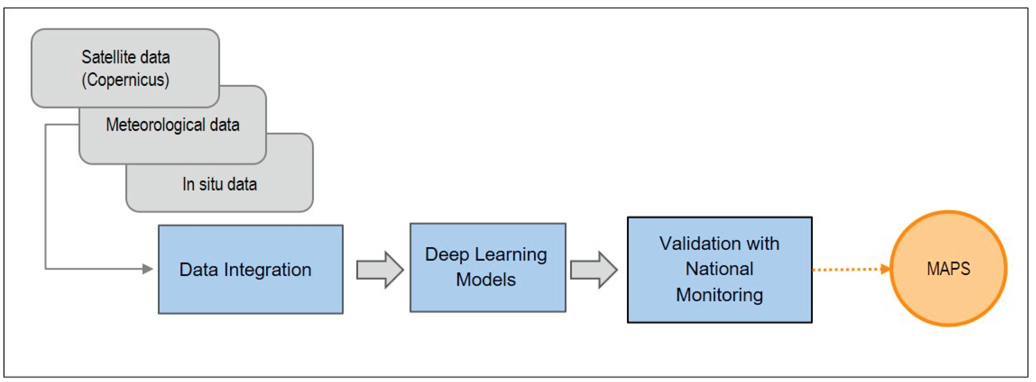
Figure 2.
Methodology for the green space mapping based on EO data (based on [6]).
Figure 2.
Methodology for the green space mapping based on EO data (based on [6]).
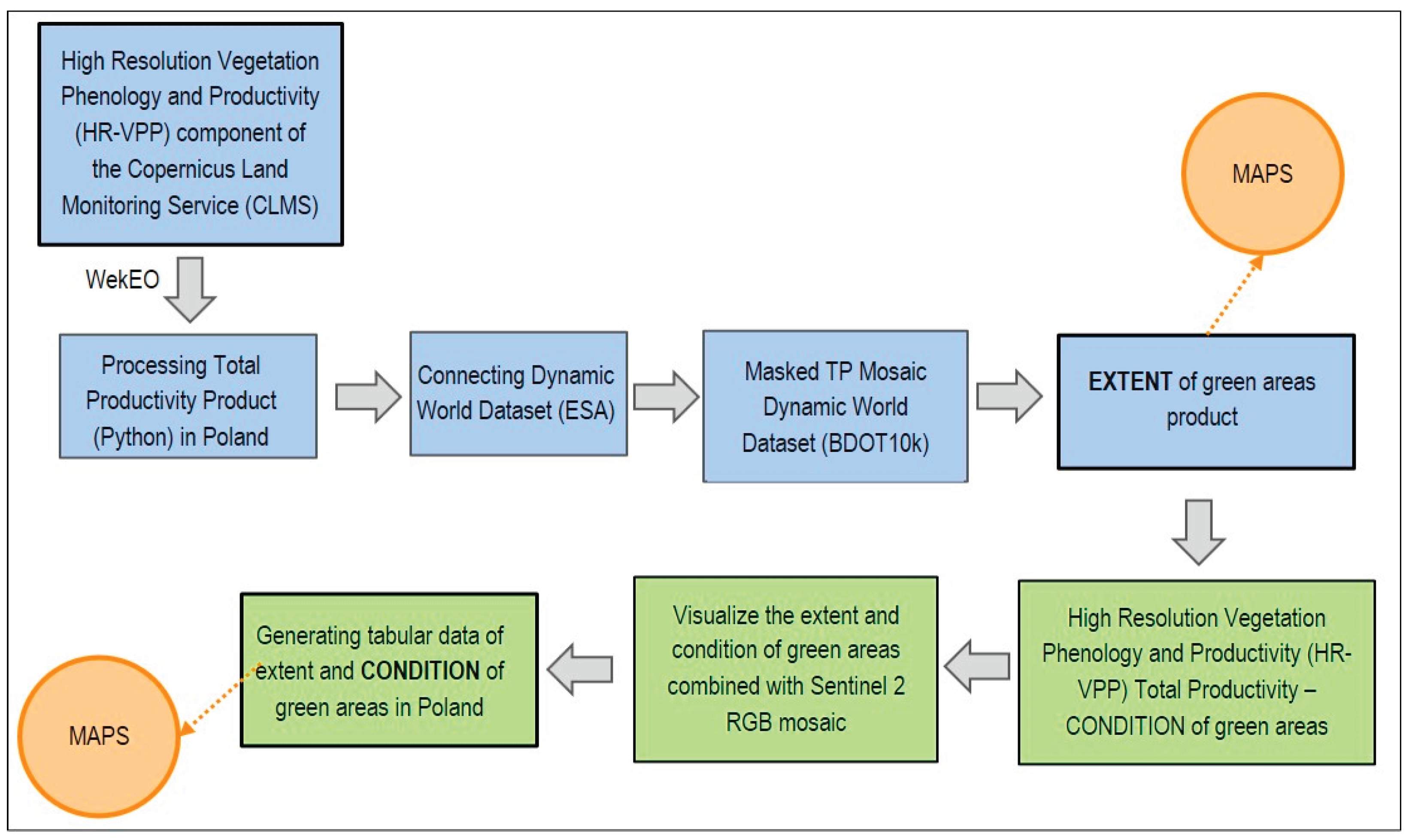
Figure 3.
Frequency of usage of cartographic presentation methods employed to visualize 11.6.2, 11.7.1 and 13.2.2 SDG indicators.
Figure 3.
Frequency of usage of cartographic presentation methods employed to visualize 11.6.2, 11.7.1 and 13.2.2 SDG indicators.
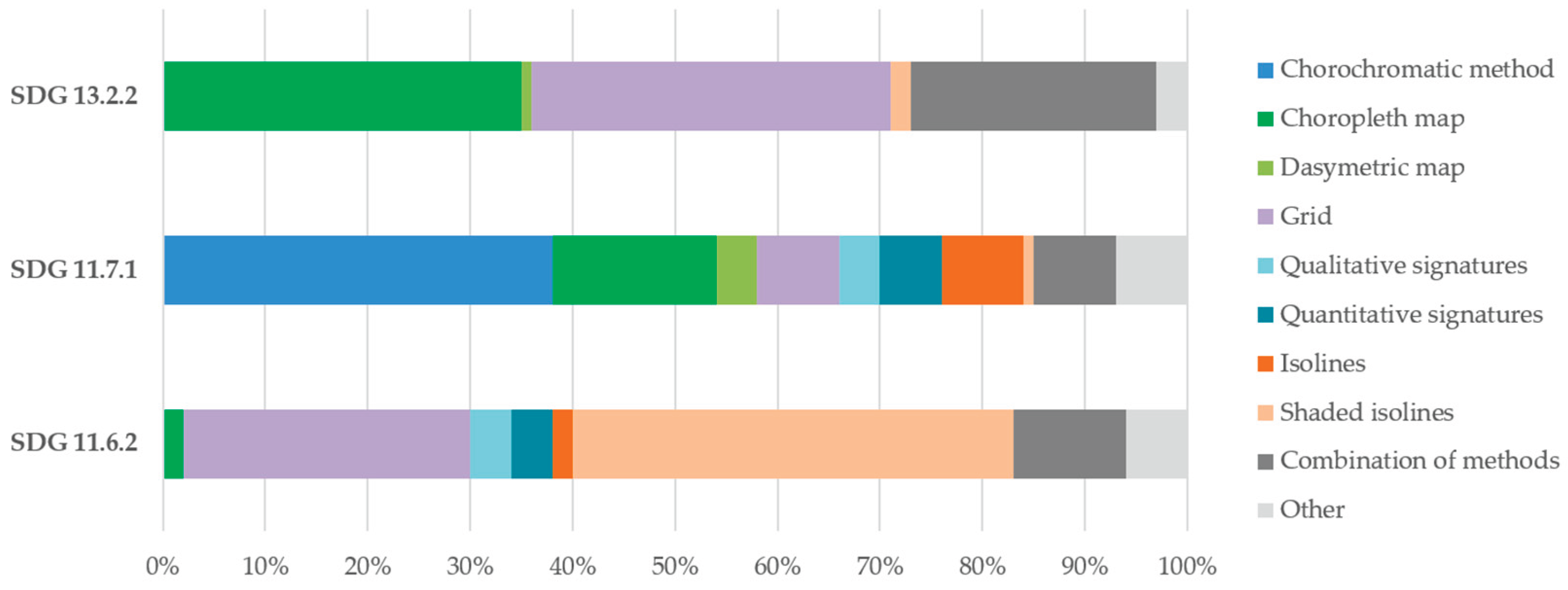
Figure 4.
The administrative division of Poland.
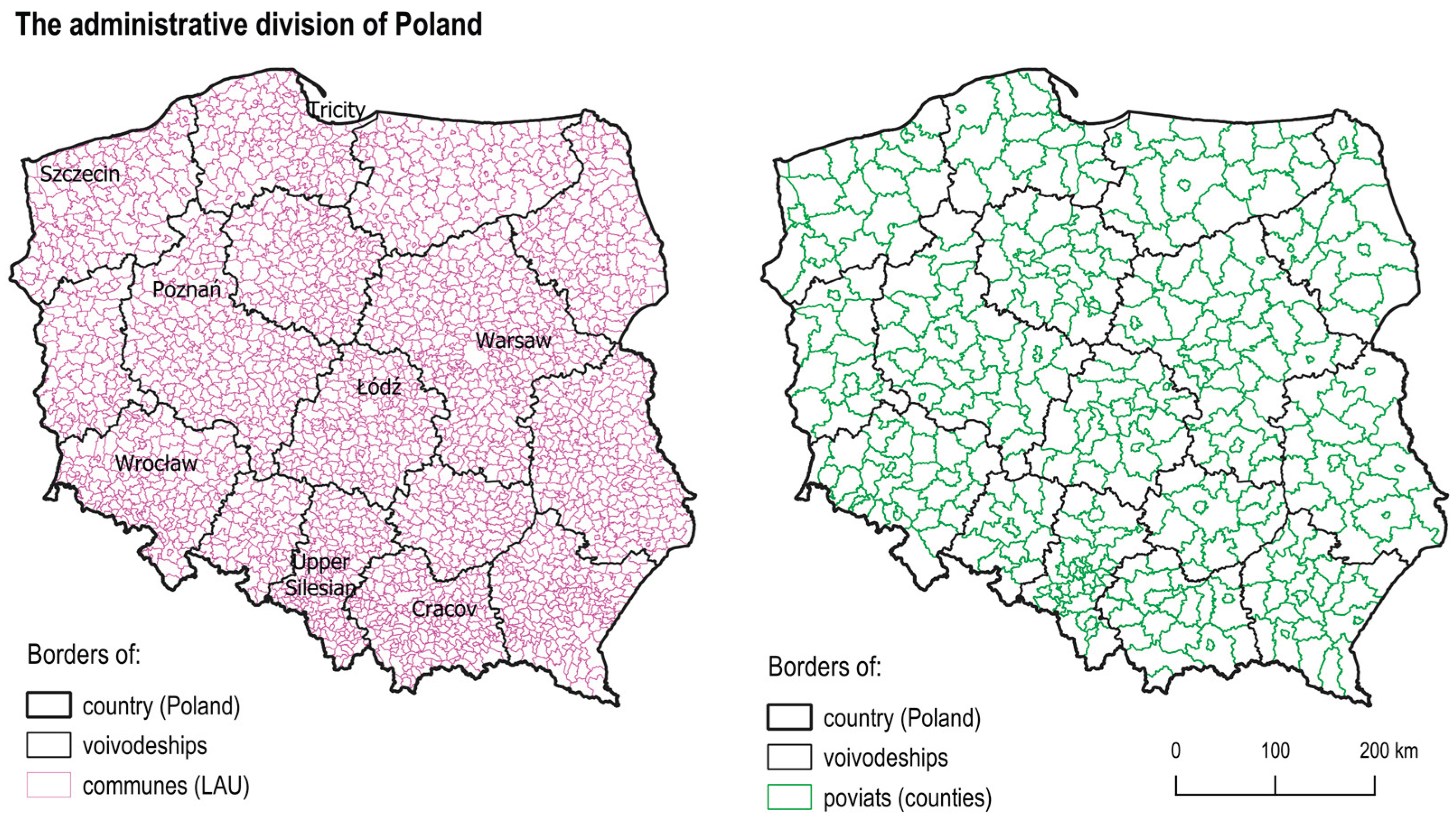
Figure 5.
Air pollution in Poland – choropleth map: yearly surface PM2.5, PM10, and NOx concentration [μg/m2] in each LAU (Local Administrative Units) in 2020. Based on the Copernicus Atmosphere Monitoring Service (CAMS) product.
Figure 5.
Air pollution in Poland – choropleth map: yearly surface PM2.5, PM10, and NOx concentration [μg/m2] in each LAU (Local Administrative Units) in 2020. Based on the Copernicus Atmosphere Monitoring Service (CAMS) product.
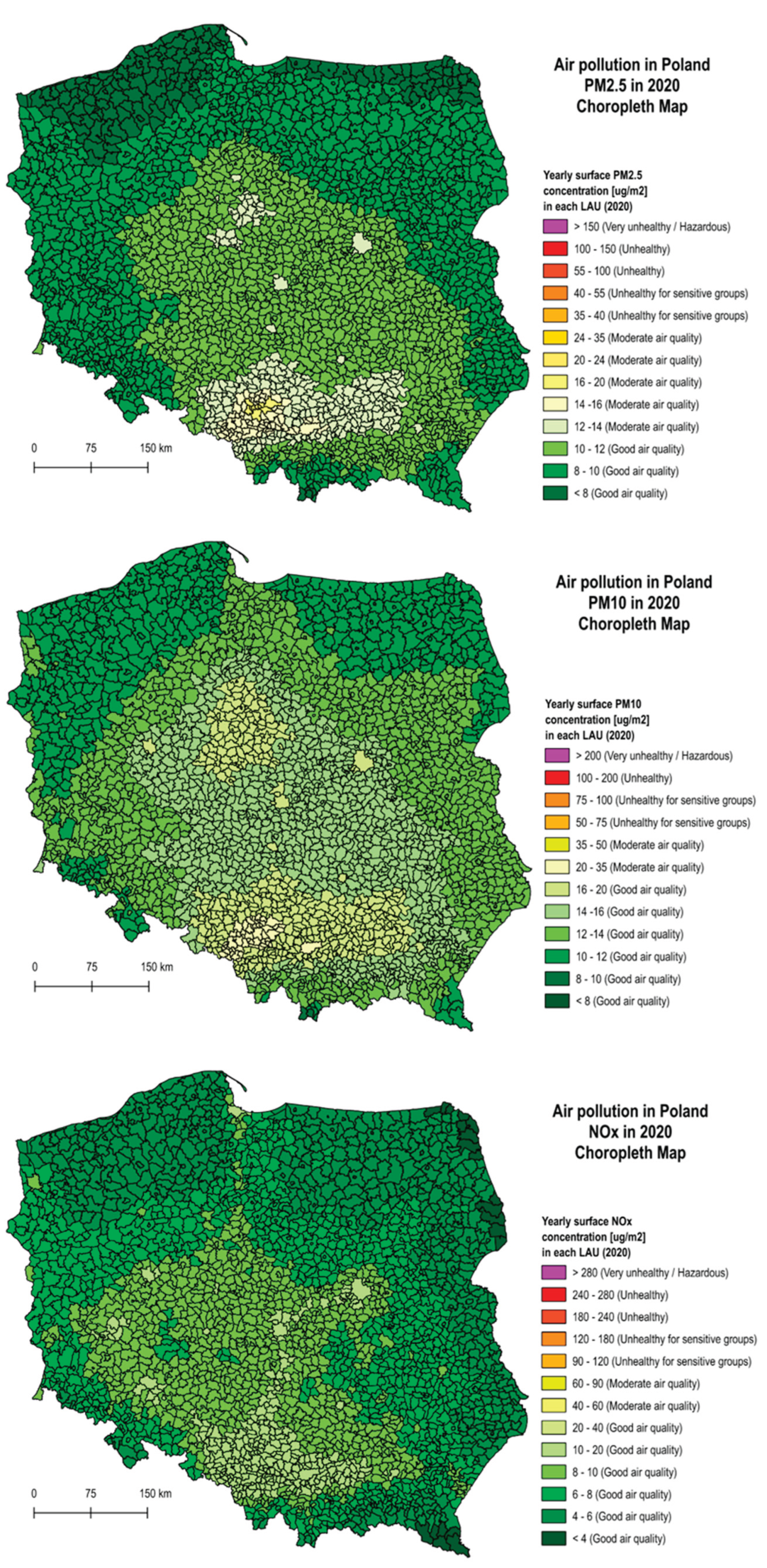
Figure 6.
Air pollution in Poland – area cartogram: yearly surface PM2.5 and PM10 concentration [μg/m2] in each LAU (Local Administrative Units) in 2020. Based on the Copernicus Atmosphere Monitoring Service (CAMS) product. The area of LAU is proportional to the number of inhabitants in a municipality in 2020.
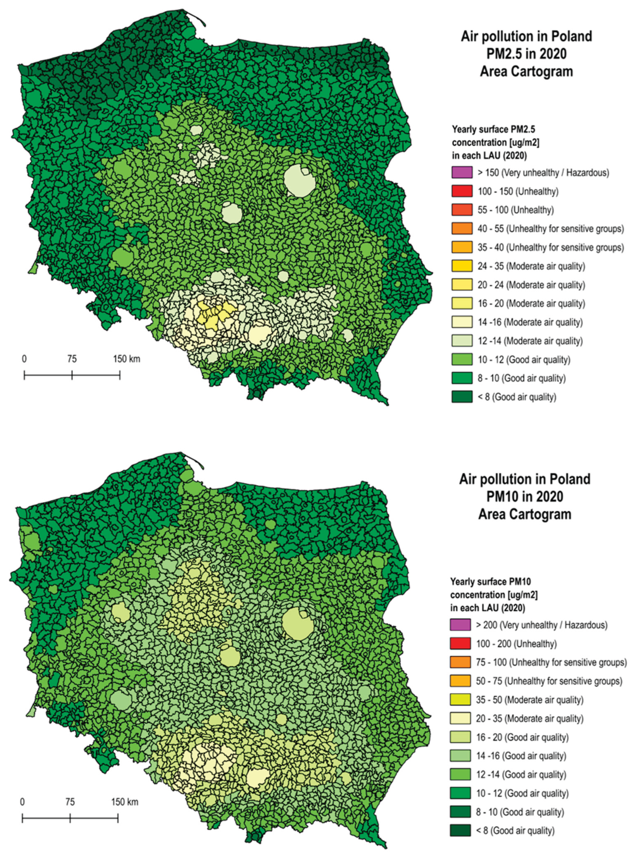
Figure 7.
Yearly surface NOx concentration [μg/m2] in each poviat in 2020 in Poland. Based on the Copernicus Atmosphere Monitoring Service (CAMS) product. Left: Choropleth map. Right: area cartogram. The area of poviat is proportional to the number of vehicles in a specific poviat in 2020.
Figure 7.
Yearly surface NOx concentration [μg/m2] in each poviat in 2020 in Poland. Based on the Copernicus Atmosphere Monitoring Service (CAMS) product. Left: Choropleth map. Right: area cartogram. The area of poviat is proportional to the number of vehicles in a specific poviat in 2020.
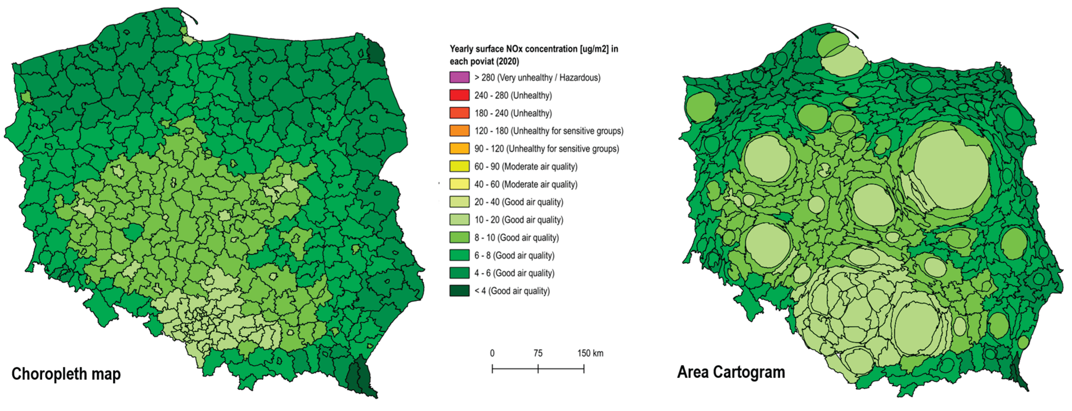
Figure 8.
Green urban areas in LAUs in 2020. Left – choropleth map, right – area cartogram (area of each commune is proportiona to area of urban spaces).
Figure 8.
Green urban areas in LAUs in 2020. Left – choropleth map, right – area cartogram (area of each commune is proportiona to area of urban spaces).
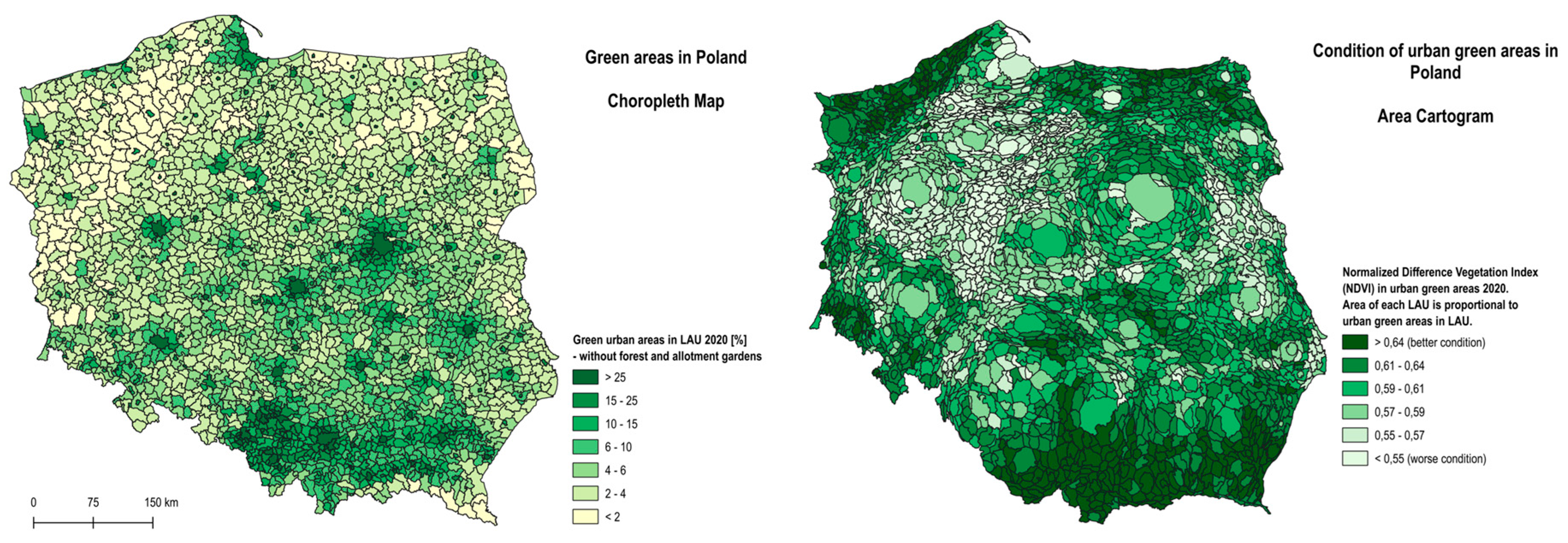
Figure 9.
Green urban areas in LAUs in 2020. Left – choropleth map, right – area cartogram (area of each commune is proportiona to number of children (aged 0–14) residing in each municipality).
Figure 9.
Green urban areas in LAUs in 2020. Left – choropleth map, right – area cartogram (area of each commune is proportiona to number of children (aged 0–14) residing in each municipality).
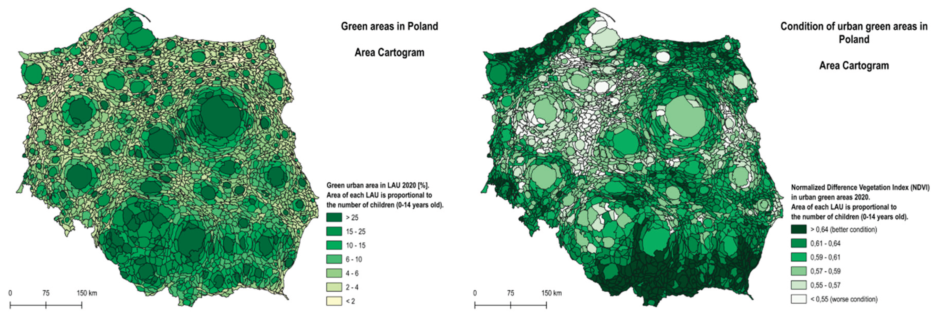

Table 1.
Air quality classification based on PM2.5, PM10, and nitrogen oxides (NOx) concentration levels (µg/m³). Based on [102].
Table 1.
Air quality classification based on PM2.5, PM10, and nitrogen oxides (NOx) concentration levels (µg/m³). Based on [102].
| Color | PM2.5 Range (µg/m³) |
PM10 Range (µg/m³) |
Nitrogen Oxides (NOₓ) Range (µg/m³) | Air Quality Description |
|---|---|---|---|---|
| Green | 0 – 12 | 0 – 20 | 0 – 40 | Good air quality |
| Yellow | 12 – 35 | 20 – 50 | 40 – 90 | Moderate air quality |
| Orange | 35 – 55 | 50 – 100 | 90 – 180 | Unhealthy for sensitive groups |
| Red | 55 – 150 | 100 – 200 | 180 – 280 | Unhealthy |
| Purple | >150 | >200 | >280 | Very unhealthy /Hazardous |
Table 2.
Software for the generation of contiguous area cartograms. The table presents the type of area cartogram (based on [105]), the name of the software, and a brief summary.
Table 2.
Software for the generation of contiguous area cartograms. The table presents the type of area cartogram (based on [105]), the name of the software, and a brief summary.
| Tools | Software / Language | Cartogram Type | Summary |
|---|---|---|---|
| ScapeToad | Java | Irregular – Gastner-Newman |
Desktop application, diffusion algorithm [107] |
| Cartogram Geoprocessing Tool | ArcGIS Toolbox | Irregular – Gastner-Newman |
Implements Gastner-Newman algorithm within ArcGIS environment |
| RecMap | R | Rectangular or Mosaic | Produces cartograms using rectangular subdivision with attribute scaling [108] |
| Tilegrams | JavaScript | Hexagonal | Uses equal-sized hexagons or squares; suitable for web presentations (Pitch Interactive) |
| cartogram 3 | Python (PyQGIS) QGIS Plugin |
Irregular – Gastner-Newman |
Integrates cartogram generation into open-source QGIS environment [109] |
| cartogram: Create Cartograms with R | R | Irregular – gridded | It is actively maintained and suitable for creating gridded cartograms [110] |
| go-cart | C++ | Irregular– Flow-Based | Create a area cartogram, using Flow-Based-Algorithm [111] |
Disclaimer/Publisher’s Note: The statements, opinions and data contained in all publications are solely those of the individual author(s) and contributor(s) and not of MDPI and/or the editor(s). MDPI and/or the editor(s) disclaim responsibility for any injury to people or property resulting from any ideas, methods, instructions or products referred to in the content. |
© 2025 by the authors. Licensee MDPI, Basel, Switzerland. This article is an open access article distributed under the terms and conditions of the Creative Commons Attribution (CC BY) license (http://creativecommons.org/licenses/by/4.0/).
Copyright: This open access article is published under a Creative Commons CC BY 4.0 license, which permit the free download, distribution, and reuse, provided that the author and preprint are cited in any reuse.


