Structural Results on the HMLasso

1. Introduction

Let X be an $n\times p$ design matrix and let $\mathbf{y}$ be an n-dimensional response. Consider the following standard linear regression model

$$\mathbf{y}=X\beta +ϵ,$$

(1)

where $ϵ$ is a noise term. The popular model focused on sparsity assumption of the regression vector. The Lasso [2] (Least absolute shrinkage and selection operator) is among the most popular procedures for estimating the unknown sparse regression vector in a high-dimensional linear model. Lasso is formulated as an ${\ell }^1$-penalized regression problem as follows:

$$\underset{\beta }{min}{\displaystyle \frac{1}{2n}}{\parallel \mathbf{y}-X\beta \parallel }_2^2+\alpha {\parallel \beta \parallel }_1$$

(2)

where $\alpha >0$ is a regularization parameter and ${\parallel ·\parallel }_1$ (resp. ${\parallel ·\parallel }_2$) is the ${\ell }^1$ (resp. ${\ell }^2$) norm. Here, we consider the case where the design matrix X contains missing data. Missing data is prevalent and inevitable, which affects not only the representativeness and quality of data but also the results of Lasso regression. Therefore, it is crucial to develop a method applicable to process missing data. HMLasso [1] was proposed to effectively address this issue and is formulated as follows:

$$\begin{array}{cc}\hfill & \underset{\Sigma }{min}{\displaystyle \frac{1}{2}}{\parallel W\odot (\Sigma -S^{\mathrm{pair}})\parallel }_{\mathrm{F}}^2\mathrm{s}.\mathrm{t}.\Sigma ⪰0\hfill \end{array}$$

(3)

$$\begin{array}{cc}\hfill & \underset{\beta }{min}{\displaystyle \frac{1}{2}}{\beta }^{\top }\widehat{\Sigma }\beta -{\rho }^{\mathrm{pair}\top }\beta +\alpha {\parallel \beta \parallel }_1,\hfill \end{array}$$

(4)

where ⊙ is Hadamard product, ${\parallel ·\parallel }_{\mathrm{F}}$ is Frobenius norm, $S^{\mathrm{pair}},W\in {\mathbb{R}}^{p\times p},{\rho }^{\mathrm{pair}}\in {\mathbb{R}}^p$ is defined using X (see Section 2 for details) and $\widehat{\Sigma }=\underset{\Sigma ⪰0}{\mathrm{argmin}}{\displaystyle \frac{1}{2}}{\parallel W\odot (\Sigma -S^{\mathrm{pair}})\parallel }_{\mathrm{F}}^2$ (i.e., $\widehat{\Sigma }$ is the solution to problem (3)). It is known that problem (4) can be equivalently written as Lasso (2), and in the literature dedicated to sparse regression the most encountered algorithm is the proximal gradient method when dealing with a sum of two convex functions. Therefore, the key to solving HMLasso is to consider how fast and accurately problem (3) can be solved.

To deal with this challenge, we consider two structural results on the HMlasso problem. The first, we show that the gradient of the objective function of (3) is Lipschitz continuous; the second, we show that the objective function of (3) is strongly convex. These results guarantee that accelerated algorithms for strongly convex functions can be applied to solve (3). Finally, we conduct numerical experiments on the real data considered in [1]. The numerical results show that the accelerated algorithm for strongly convex functions is effective for solving problem (3).

2. Preliminaries

This section reviews basic definitions, facts, and notation that will be used throughout the paper.

For two matrices $A,B\in {\mathbb{R}}^{n\times p}$, their Hadamard product $A\odot B$ is defined by

$${\left(A\odot B\right)}_{jk}{A}_{jk}{B}_{jk}.$$

The Frobenius inner product is defined by ${〈A,B〉}_{\mathrm{F}}\mathrm{tr}\left(A{B}^{\top }\right)$. The Frobenius norm of A is defined by

$${\parallel A\parallel }_{\mathrm{F}}\sqrt{{〈A,A〉}_{\mathrm{F}}}=\sqrt{\sum _j^n\sum _k^p{A}_{jk}^2}.$$

${\mathbb{S}}^p$ denotes the set of symmetric matrices of size $p\times p$. We write $A⪰0$ (resp. $A\succ 0$) to denote that $A\in {\mathbb{S}}^p$ is positive semidefinite (resp. positive definite). ${\mathbb{S}}_{+}^p$ denotes the set of positive semidefinite matrices.

Let $\mathcal{D}\subset {\mathbb{R}}^{p\times p}$. The indicator function $i_{\mathcal{D}}:{\mathbb{R}}^{p\times p}\to (-\infty ,\infty ]$ of $\mathcal{D}$ is defined by

$$i_{\mathcal{D}}\left(B\right)\left\{\begin{array}{cc}0\hfill & (B\in \mathcal{D});\hfill \\ \infty \hfill & \left(\mathrm{otherwise}\right).\hfill \end{array}\right.$$

Let $f:{\mathbb{R}}^{p\times p}\to (-\infty ,\infty ]$ be a proper and convex function. The proximal mapping ${\mathrm{prox}}_{\gamma f}\left(x\right)$ of f is defined by

$${\mathrm{prox}}_f\left(\Sigma \right)\underset{W\in {\mathbb{R}}^{p\times p}}{\mathrm{argmin}}\left\{f\left(W\right)+{\displaystyle \frac{1}{2}}{\parallel W-\Sigma \parallel }_{\mathrm{F}}^2\right\}.$$

Let $\Sigma \in {\mathbb{S}}^p$. Then there exist a diagonal matrix $\Lambda \in {\mathbb{R}}^{p\times p}$ and a $p\times p$ orthogonal matrix U such that $\Sigma =U\Lambda U^{\top }$. Let $P_{{\mathbb{S}}_{+}^p}$ be the matric projection from ${\mathbb{S}}^p$ onto ${\mathbb{S}}_{+}^p$. Then, the following holds (see for example [3], [Example 29.31], [4] [Theorem 6.3]):

$$P_{{\mathbb{S}}_{+}^p}\left(\Sigma \right)=U{\Lambda }_{+}{U}^{\top },$$

(5)

where ${\Lambda }_{+}$ is the diagonal matrix obtaind from $\Lambda$ by setting the negative entries to 0.

Let $X\in {\mathbb{R}}^{n\times p}$ be a design matrix. Set

$$I_{jk}\{i:X_{ij}\mathrm{and}{X}_{ik}\mathrm{are}\mathrm{observed}\}$$

and let $n_{jk}$ be the number of elements of $I_{jk}$. We define matricies $S^{\mathrm{pair}}$ and W as follows:

$$\begin{array}{c}\hfill {\left(S^{\mathrm{pair}}\right)}_{jk}\left\{\begin{array}{cc}{\displaystyle \frac{1}{n_{jk}}}\sum _{i\in I_{jk}}{x}_{ij}{x}_{ik}\hfill & (I_{jk}\ne ⌀)\hfill \\ 0\hfill & (I_{jk}=⌀)\hfill \end{array}\right.,{\left(W\right)}_{jk}{\displaystyle \frac{n_{jk}}{n}}.\end{array}$$

(6)

Let $L\in [0,\infty )$ and let $h:{\mathbb{R}}^{p\times p}\to \mathbb{R}\cup \{\infty \}$ be a differentiable function. The gradient $\nabla h$ of h is said to be L-Lipschitz continuous if

$$\parallel \nabla h\left({\Sigma }_1\right)-\nabla h\left({\Sigma }_2\right){\parallel }_{\mathrm{F}}\le L{\parallel {\Sigma }_1-{\Sigma }_2\parallel }_{\mathrm{F}}(\forall {\Sigma }_1,{\Sigma }_2\in {\mathbb{R}}^{p\times p}).$$

(7)

This condition is often called L-smoothness in the literature. Let $h:{\mathbb{R}}^{p\times p}\to \mathbb{R}$ be L-smooth on ${\mathbb{R}}^{p\times p}$, Then, we can upper bound the function h as

$$h\left({\Sigma }_1\right)\le h\left({\Sigma }_2\right)+〈\nabla h\left({\Sigma }_2\right),{\Sigma }_1-{\Sigma }_2〉+{\displaystyle \frac{L}{2}}{\parallel {\Sigma }_1-{\Sigma }_2\parallel }_{\mathrm{F}}^2(\forall {\Sigma }_1,{\Sigma }_2\in {\mathbb{R}}^{p\times p})$$

(8)

( see for example [5] [Theorem 5.8], [6] [Theorem A.1]).

Let $\mu \in (0,\infty )$ and let $g:{\mathbb{R}}^{p\times p}\to \mathbb{R}\cup \{+\infty \}$. g is said to be $\mu$-strongly convex if for each ${\Sigma }_1,{\Sigma }_2\in {\mathbb{R}}^{p\times p}$ and $\lambda \in (0,1)$, we have

$$g(\lambda {\Sigma }_1+(1-\lambda ){\Sigma }_2)\le \lambda g\left({\Sigma }_1\right)+(1-\lambda )g\left({\Sigma }_2\right)-{\displaystyle \frac{\mu }{2}}\lambda (1-\lambda ){\parallel {\Sigma }_1-{\Sigma }_2\parallel }_{\mathrm{F}}^2.$$

(9)

Suppose that g is $\mu$-strongly convex and differentiable. Then (9) is equivalent to the following condition:

$$〈\nabla g\left({\Sigma }_1\right)-\nabla g\left({\Sigma }_2\right),{\Sigma }_1-{\Sigma }_2〉\ge \mu {\parallel {\Sigma }_1-{\Sigma }_2\parallel }_{\mathrm{F}}^2(\forall {\Sigma }_1,{\Sigma }_2\in {\mathbb{R}}^{p\times p}).$$

(10)

3. Main Results

In this section, we present two structural results on the HMlasso problem (3).

Define $f\left(\Sigma \right){\displaystyle \frac{1}{2}}{\parallel W\odot (\Sigma -S^{\mathrm{pair}})\parallel }_{\mathrm{F}}^2$. In this case, the gradient $\nabla f$ of f is described as the following:

$$\nabla f\left(\Sigma \right)=\nabla \left({\displaystyle \frac{1}{2}}{\parallel W\odot (\Sigma -S^{\mathrm{pair}})\parallel }_{\mathrm{F}}^2\right)=W\odot W\odot (\Sigma -S^{\mathrm{pair}})$$

(11)

(see [1]).

3.1. Lipschitz continuity

The first structural result deals with the gradient of the objective function in (3). We show the Lipschitz continuity of $\nabla f$.

Lemma 1. 

The gradient $\nabla f$ of f is Lipschitz continuous and its Lipschitz constant is ${\parallel W\odot W\parallel }_{\mathrm{F}}$.

Proof. 

$$\begin{array}{cc}\hfill \parallel \nabla f\left({\Sigma }_1\right)-\nabla f\left({\Sigma }_2\right){\parallel }_{\mathrm{F}}^2& =\parallel W\odot W\odot ({\Sigma }_1-S^{\mathrm{pair}})-W\odot W\odot ({\Sigma }_2-S^{\mathrm{pair}}){\parallel }_{\mathrm{F}}^2\hfill \\ \hfill & =\parallel W\odot W\odot ({\Sigma }_1-{\Sigma }_2){\parallel }_{\mathrm{F}}^2\hfill \\ \hfill & =\sum _{j=1}^p\sum _{k=1}^p{\left(W_{jk}^2({\Sigma }_{1jk}-{\Sigma }_{2jk})\right)}^2.\hfill \end{array}$$

On the other hand,

$$\begin{array}{cc}\hfill {\parallel W\odot W\parallel }_{\mathrm{F}}^2{\parallel {\Sigma }_1-{\Sigma }_2\parallel }_{\mathrm{F}}^2& =\underset{\overline{\alpha }}{\underbrace{\sum _{j=1}^p\sum _{k=1}^p{W}_{jk}^4}}·\sum _{j=1}^p\sum _{k=1}^p{\left({\Sigma }_{1jk}-{\Sigma }_{2jk}\right)}^2.\hfill \end{array}$$

This implies

$$\begin{array}{cc}\hfill {\parallel W\odot W\parallel }_{\mathrm{F}}^2\parallel {\Sigma }_1-{\Sigma }_2{\parallel }_{\mathrm{F}}^2-{\parallel \nabla f\left({\Sigma }_1\right)-\nabla f\left({\Sigma }_2\right)\parallel }_{\mathrm{F}}^2& =\sum _{j=1}^p\sum _{k=1}^p\left(\overline{\alpha }-W_{jk}^4\right){\left({\Sigma }_{1jk}-{\Sigma }_{2jk}\right)}^2\hfill \\ \hfill & \ge 0,\hfill \end{array}$$

where the last inequality follows from $\overline{\alpha }-W_{jk}^4\ge 0$ for any j and k. Hence

$$\begin{array}{c}\hfill \parallel \nabla f\left({\Sigma }_1\right)-\nabla f\left({\Sigma }_2\right){\parallel }_{\mathrm{F}}\le {\parallel W\odot W\parallel }_{\mathrm{F}}{\parallel {\Sigma }_1-{\Sigma }_2\parallel }_{\mathrm{F}}.\end{array}$$

   □

3.2. Strong monotonicity

We next consider the strong monotonicity of f. This is our second result.

Lemma 2. 

f is ${min}_{l,m}{(W\odot W)}_{l,m}$-strongly convex.

Proof. 

We show (10) with constant ${min}_{l,m}{(W\odot W)}_{l,m}$. Let ${\Sigma }_1,{\Sigma }_2\in {\mathbb{R}}^{p\times p}$.

$$\begin{array}{cc}\hfill 〈\nabla f\left({\Sigma }_1\right)-\nabla f\left({\Sigma }_2\right),{\Sigma }_1-{\Sigma }_2〉& =〈W\odot W\odot ({\Sigma }_1-{\Sigma }_2),{\Sigma }_1-{\Sigma }_2〉\hfill \\ \hfill & =\sum _{j=1}^p\sum _{k=1}^p{W}_{jk}^2{({\Sigma }_{1jk}-{\Sigma }_{2jk})}^2\hfill \\ \hfill & \ge \sum _{j=1}^p\sum _{k=1}^p\underset{j,k}{min}{(W\odot W)}_{j,k}{({\Sigma }_{1jk}-{\Sigma }_{2jk})}^2\hfill \\ \hfill & =\underset{l,m}{min}{(W\odot W)}_{l,m}{\parallel {\Sigma }_1-{\Sigma }_2\parallel }_{\mathrm{F}}^2,\hfill \end{array}$$

where the second to last inequality follows from $W_{jk}^2\ge {min}_{l,m}{(W\odot W)}_{l,m}$ for any j and k. This implies that f is ${min}_{l,m}{(W\odot W)}_{l,m}$-strongly convex.    □

Remark 1. 

From Lemmas 1 and 2, the objective function of (3) is strongly convex and has Lipschitz gradient. It should be noted that we can guarantee faster convergence than just on regular convex function is if we know the objective function is strongly convex and it is smooth (see for example [6]).

4. Numerical Experiments

In this section, we consider a strongly convex variant of FISTA [6] [Algorithm 19] to solve problem (3).

4.1. Strongly convex FISTA

Let $f:{\mathbb{R}}^{p\times p}\to \mathbb{R}$ be an L-smooth and $\mu$-strongly convex function with $\mathrm{dom}\left(f\right)={\mathbb{R}}^{p\times p}$, and let $h:{\mathbb{R}}^{p\times p}\to \mathbb{R}\cup \{\infty \}$ be a convex function with $\{\Sigma :h(\Sigma )<\infty \}\ne \varnothing$. We consider the problem of minimizing sum of f and h:

$$\underset{\Sigma \in {\mathbb{R}}^{p\times p}}{min}f\left(\Sigma \right)+h\left(\Sigma \right).$$

(12)

In this setting, forward-backward splitting strategies were introduced as classical methods for solving (12). In the context of acceleration methods, the fast iterative shrinkage threshold algorithm (FISTA) was introduced by Beck and Teboulle [7] using the idea of forward-backward splitting. This topc is addressed in many references, and we refer to [3,5,6].

Here, we focus on the following strongly convex variant of FISTA involving backtracking investigated in [6].

Algorithm 1: Strongly convex FISTA [6] [Algorithm 19]

Input:  An initial point ${\Sigma }_0\in {\mathbb{R}}^{p\times p}$, and initial estimate $L_0>\mu$. 1: Initialize${\Phi }_0={\Sigma }_0$, $t_0=0$, and some $\alpha >1$. 2: for$k=0,\dots$do 3:    $L_{k+1}=L_k$ 4:    while do 5:      $q_{k+1}=\mu /L_{k+1}$ 6:      $t_{k+1}={\displaystyle \frac{2t_k+1+\sqrt{4t_k+4q_{k+1}{t}_k^2+1}}{2(1-q_{k+1})}}$ 7:      set ${\tau }_k={\displaystyle \frac{(t_{k+1}-t_k)(1+q_{k+1}{t}_k)}{t_{k+1}+2q_{k+1}{t}_k{t}_{k+1}-q_k{t}_k^2}}$ and ${\delta }_k={\displaystyle \frac{t_{k+1}-t_k}{1+q_{k+1}{t}_{k+1}}}$ 8:      ${\Psi }_k={\Sigma }_k+{\tau }_k({\Phi }_k-{\Sigma }_k)$ 9:      ${\Sigma }_{k+1}={\mathrm{prox}}_{h/L_{k+1}}({\Psi }_k-{\displaystyle \frac{1}{L_{k+1}}}\nabla f\left({\Psi }_k\right))$ 10:      ${\Phi }_{k+1}=(1-q_{k+1}{\delta }_k){\Phi }_k+q_{k+1}{\delta }_k{\Psi }_k+{\delta }_k({\Sigma }_{k+1}-{\Psi }_k)$ 11:      if $f\left({\Sigma }_{k+1}\right)\le f\left({\Sigma }_k\right)+〈\nabla f\left({\Sigma }_k\right),{\Sigma }_{k+1}-{\Sigma }_k〉+{\displaystyle \frac{L_{k+1}}{2}}{\parallel {\Sigma }_{k+1}-{\Sigma }_k\parallel }_{\mathrm{F}}^2$ holds then 12:         $\mathbf{break}\{k\mathrm{will}\mathrm{be}\mathrm{incremented}.\}$ 13:      else 14:         $L_{k+1}=\alpha L_{k+1}\{\mathrm{Recompute}\mathrm{new}{L}_{k+1}.\}$ 15:      end if 16:    end while 17: end for Output:  An approximate solution ${\Sigma }_{k+1}$

Remark 2. 

We demonstrate how strongly convex FISTA can be applied to (3). Set

$$f\left(\Sigma \right){\displaystyle \frac{1}{2}}{\parallel W\odot (\Sigma -S^{\mathrm{pair}})\parallel }_{\mathrm{F}}^2\mathrm{and}h\left(\Sigma \right)i_{{\mathbb{S}}_{+}^p}\left(\Sigma \right).$$

In this case, problem (3) is the special instanse of problem (12). The gradient $\nabla f$ can be computed by (11). Moreover, the proximal mapping ${\mathrm{prox}}_h$ is $P_{{\mathbb{S}}_{+}^p}$ (see for example [3], Example 12.25) and hence the computation in the algorithm is simple.

4.2. Residential Building Dataset

We compared the performance of HMLasso (3) with the strongly convex FISTA (SCFISTA) and the alternating direction multiplier method (ADMM) used in [6]. All experiments are conducted on a PC with Apple M1 Max CPU and 32GB RAM. Methods are implemented with MATLAB (R2025a).

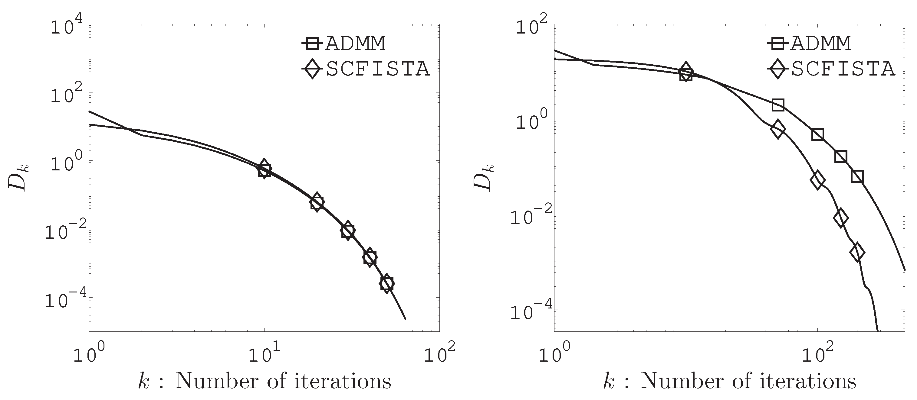
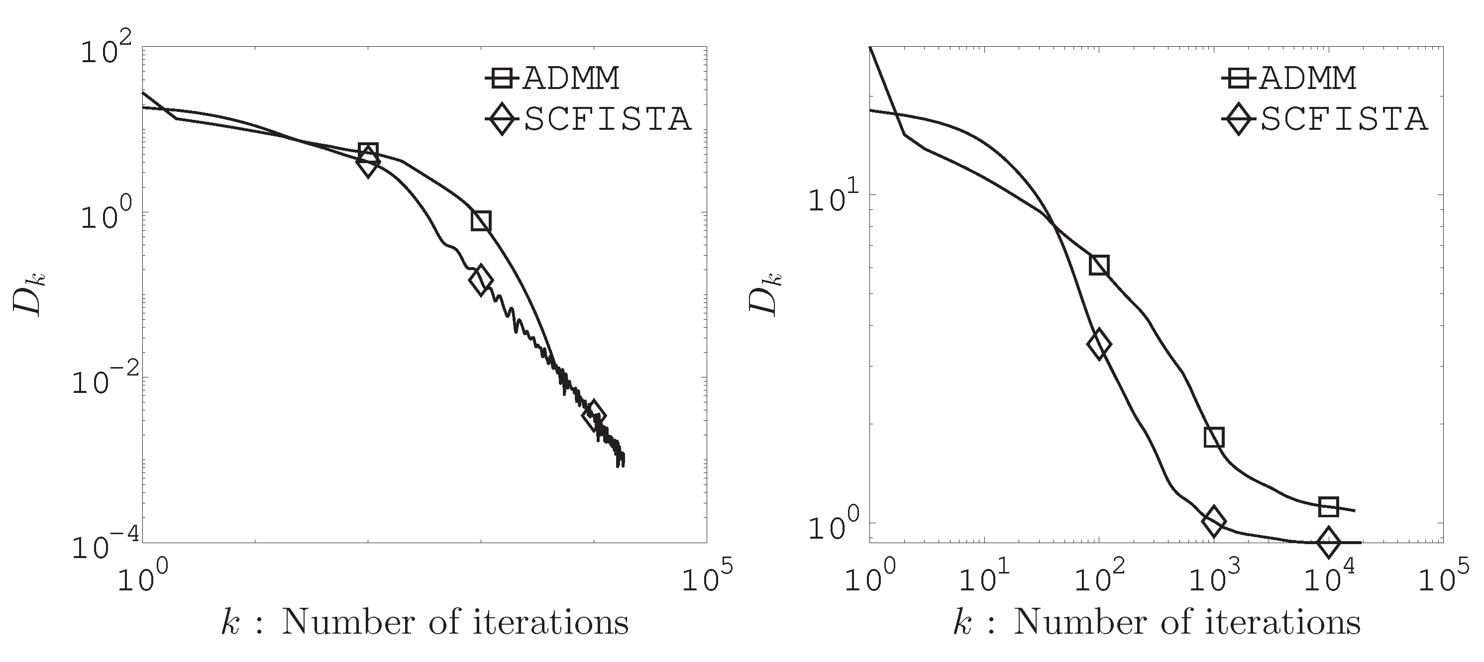
The numerical experiment uses actual residential building dataset from the UCI Data Repository1. The data consisted of $n=300$ samples and $p=27$ variables. We set the average missing rates to $20\%$, $40\%$, $60\%$ and $80\%$. As choices for $L_0$, $\alpha$ and $\mu$ occuring in algorithm, we let $L_{0}1$, $\alpha 1.1$ and $\mu {min}_{l,m}{(W\odot W)}_{l,m}$. We chose 10 random initial points ${\Sigma }_0^{\left(i\right)}\in {\mathbb{R}}^{p\times p}$ ($i=1,2,\dots ,10$) and all entries at the initial point are defined from a standard normal distribution. Figures demonstrate the following function

$$D_k^{\left(i\right)}{\parallel {\Sigma }_k^{\left(i\right)}-{\Sigma }_{\mathrm{cvx}}\parallel }_{\mathrm{F}}\mathrm{and}{D}_k(1/10)\sum _{i=1}^{10}{D}_k^{\left(i\right)},$$

(13)

where ${\Sigma }_{\mathrm{cvx}}$ denotes the solution obtained by cvx2 and $\left\{{\Sigma }_k^{\left(i\right)}\right\}$ is the sequence generated by ${\Sigma }_0^{\left(i\right)}$ and each of SCFISTA and ADMM.

Figure 1 and Figure 2 show the computation results of the relation between the distance to a solution and iteration number. As we can see from these figures, SCFISTA and ADMM converge to the solution as the number of iterations increases. Furthermore, we found it more effective to solve the HMLasso problem using the acceleration algorithm for strongly convex functions.

5. Conclusions

In this paper we present two structural results on the HMlasso problem, covering Lipschitz continuity of the gradient of the objective function and strong convexity of the objective function. These results allow existing acceleration algorithms for strongly convex functions to be applied to solve the HMLasso problem. Our numerical experiments suggest that accelerated algorithms for strongly convex functions are computationally attractive.

References

- Takada, M.; Fujisawa, H.; Nishikawa, T. HMLasso: Lasso with High Missing Rate. Proceedings of the Twenty-Eighth International Joint Conference on Artificial Intelligence (IJCAI) 2019, 3541–3547. [Google Scholar]
- Tibshirani, R. Regression shrinkage and selection via the Lasso. J. R. Stat. Soc. Ser. B. Stat. Methodol. 1996, 58, 267–288. [Google Scholar] [CrossRef]
- Bauschke, H.H.; Combettes, P.L. Convex Analysis and Monotone Operator Theory in Hilbert Spaces, 2nd ed.; Springer: CMS Books in Mathematics, 2017. [Google Scholar]
- Escalante, R.; Raydan, M. Alternating Projection Methods; SIAM: Philadelphia, PA, USA, 2011. [Google Scholar]
- Beck, A. First-order Methods in Optimization; SIAM: MOS-SIAM Series on Optimization, USA, 2017. [Google Scholar]
- d’Aspremont, A.; Scieur, D.; Taylor, A. Acceleration Methods; Now Publishers: Fundations and Trends in Optimizaion, 2021. [Google Scholar]
- Beck, A.; Teboulle, M. A fast iterative shrinkage-thresholding algorithm for linear inverse problems. SIAM J. Imag. Sci., 2009, 2, 183–202. [Google Scholar] [CrossRef]