
Submitted:
16 November 2023
Posted:
16 November 2023
You are already at the latest version
Abstract
We present a new penalized method for estimation in sparse logistic regression models with group structure. Group sparsity suggests us to consider the Group Lasso penalty. Being different from penalized log-likelihood estimation, our method can be viewed as a penalized weighted score function method. Under some mild conditions, we provide non-asymptotic oracle inequalities promoting group sparsity of predictors. A modified block coordinate descent algorithm based on a weighted score function is also employed. The net advantage of our algorithm over the existing Group Lasso-type procedures is that the tuning parameter can be pre-specified. The simulations show that this algorithm is considerably faster and more stable than competing methods. Finally, we illustrate our methodology with two real data sets.
Keywords:
high-dimensional data
; non-asymptotic inequality
; logistic regression
; variable selection
; block coordinate descent algorithm
1. Introduction
Logistic regression models are a powerful and popular technique for modeling the relationship between the predictors and a categorical response variable. Let be independent pairs of observed data which are realizations of random vector , with dimensional predictors and univariate binary response variable . is assumed to satisfy
where is a regression vector to be estimated. We are especially concerned with a sparse logistic regression problem when the dimension p is high and the sample size n might be small, the so-called "small n, large p" framework, which is a variable selection problem for high-dimensional data.
When dealing with high-dimensional data, there are usually two important considerations: model sparsity and prediction accuracy. The Lasso [1] was proposed to address these two objectives since Lasso can determine submodels with a moderate number of parameters that still fit the data adequately. There are also other similar methods include SCAD [2], elastic net [3], Dantzig selector [4], MCP [5] and so on. In high-dimensional logistic regression models, the topics for Lasso study range from the asymptotic results, including the consistency and asymptotic distribution of the estimator, e.g., Huang et al. [6], Bianco et al. [7], to the non-asymptotic results, including the non-asymptotic oracle inequalities on the estimation and prediction errors, e.g., Abramovich et al. [8], Huang et al. [9] and Yin [10].
In many applications, predictors can often be thought of as grouped. For example, in genome-wide association studies (GWAS), genes usually do not act individually, but are reflected in the covariation of several genes with each other. Or in histologically normal epithelium (NlEpi) studies, we need to consider the non-linear effects of genes for microarray data. Similar to the Lasso, considering this grouped information in the modeling process should improve the interpretability and the accuracy of the model. Yuan and Lin [11] proposed an extension of the Lasso, called the Group Lasso, which imposes an penalty to individual groups of variables and then an penalty to the resulting block norms, rather than only an penalty to individual variables. Suppsose and in model (1) are divided into g known groups, where we consider a partition of into groups and denote the cardinality of a group by , , , , . We wish to achieves sparsity at the level of groups, i.e., to such that for some of the groups . When using high-dimensional logistic regression models, the Group Lasso provides an estimator for :
where is a tuning parameter which controls the amount of penalization, is used to normalize across groups of different sizes, and denotes the norm of a vector. Meier et al. [12] established the asymptotic consistency theory of the Group Lasso for logistic regression, Wang et al. [13] analyzed the rates of convergence, Blazere et al. [14] stated oracle inequalities and Kwemou [15] studied non-asymptotic oracle inequalities. Other important references are the works of Nowakowski et al. [16] and Zhang et al. [17]. In terms of computational algorithms, Meier et al. [12] applied the block coordinate descent algorithm of Tseng [18] to Group Lasso for logistic regression, Breheny and Huang [19] proposed the Group descent algorithm. These approaches are sufficiently fast for computing the exact coefficients at those selected values of .
However, it is well known that the Lasso (or the Group Lasso) in linear regression models, the respective optimal values of tuning parameter depend on the unknown parameter , the homogeneous noise variance, and its the accurate estimation is generally more difficult when . To solve this problem, Belloni et al. [20] proposed square-root Lasso, which removed this unknown parameter by using a weighted score function (i.e. the square root of empirical loss function). Bunea et al. [21] extended the ideas behind the square-root Lasso for group selection and developed the Group square-root Lasso. Inspired by Group square-root Lasso, we propose a new penalized weighted score function method, which alternatively replaces the original score function (i.e. the gradient of negative loglikelihood function) with a weighted score function (Huang and Wang [22]), to study sparse logistic regression with Group Lasso penalty. We get convergence rates for the estimation error and provide a direct choice for the tuning parameter. Moreover, we propose a modified block coordinate descent algorithm based on the weighted score function, which greatly optimizes the computational complexity.
The framework of this paper is as follows. In Section 2, we apply this idea behind the Group square-root Lasso to sparse logisitic models and develop our method, the penalized weighted score function method. In Section 3, we propose asymptotic bounds for our new estimator and a direct selection for the tuning parameter. In Section 4, we provide weighted block coordinate descent algorithm. In Section 5, numerical simulations show the advantages of our algorithm in terms of selection effects and computational time. In Section 6, we present real data for genes and musk to support the simulation and theoretical results. The Section 7 concludes our work. All proofs are given in Appendix.
Throughout the paper, denote by the non-zero coordinate of and let be the number of non-zero elements of . For all and subset I, we denote by that has the same coordinates as on I and zero coordinates on the complement of I. For a function , we denote by its gradient and its Hessian matrix at . Define the norm of any vector v as and for any vector with group structures, denote the block norm of for any as . In particular, indicates the number of non-zero groups, represents the form of Group Lasso, denotes norm, and means the largest norm of all groups. Moreover denotes the cumulative distribution function of the standard normal distribution.
2. Penalized weighted score function method
Recall model (1), the loss function (i.e. the negative loglikelihood) is given by
leading to the score function
Note that the solution of model (2) satisfies KKT conditions defined as follows
for all . The left side of equation (3) is the score function for logistic regression with group structure, which shows that is actually a penalized score function estimator. To obtain a good estimator, usually we require that the inequality for all and some constant holds with high probability (Meier et al. [12] and Kwemou [15]). However, the random part for , the score function valued at , has variance , which is also the variance of the binary random variable . Obviously, binary noises are not homogeneous like noises of the linear regression models, a unique tuning parameter for all of the different coefficient is not a good choice.
We apply the idea from Group square-root Lasso to solve the above problem on choosing tuning parameter, and develop our method as follows. Huang and Wang [22] formed a class of root-consistent estimating functions by weighted score function for logistic regression
where is the weighted function of . This requires choosing a suitable weighed function to ensure that is almost integrable for . Then, replacing the score function in equation (3) with the weighted score function, we develop a penalized weighted score function estimate , which is a solution of the following equation:
Let be the loss function corresponding to the weighted score function (4), the solution to Equation (5) is equivalent to solve the following optimization problem:
Our method is motivated by Bunea et al. [21] minimization of the Group square-root Lasso for linear model:
where and . When is non-zero, the Group square-root Lasso estimator satisfies the KKT condition
Compared with the KKT conditions for Group square-root Lasso and Group Lasso, the Group square-root Lasso adds the weighted function to estimate the homogeneous noise variance, which allows the tuning parameter independent of the homogeneous noise variance. Thus, the Group square-root Lasso is able to estimate for the grouped variables and direct choice for the tuning parameter simultaneously.
A drawback of Group square-root Lasso is that it can only directly select the tuning parameter in a linear regression models. However, in logistic regression models, there is no direct way to select the tuning parameter. The penalized weighted score function method implements this scheme. We will discuss this in more detail in the next section.
3. Statistical properties
In this section, we will establish non-asymptotic oracle inequalities for the penalized weighted score function estimate and give a direct choice for tuning parameter.
Throughout this paper, we consider a fixed design setting (i.e., are consider deterministic), and we make the following assumptions:
- (A1)
- There exists a positive constant such that .
- (A2)
- The satisfy that , and for .
- (A3)
- There exists such that
- (A4)
- Let be a convex three times differentiable function such that for all , the function satisfies for all , , where is a constant.
The assumption (A1) strictly controls the bounds of predictors, since the real data we collected was often bounded. The assumption (A2) controls the sparsity of the data and the lower bound on the probability that the non-asymptotic property holds. The assumption (A3) makes sure the variance of each component of is bounded with choosing a suitable weighted function . The assumption (A4) is similar to the proposition 1 proposed by Bach [23]. Under the assumption (A4), we can obtain lower and upper Taylor expansions of the loss function , using which we can derive non-asymptotic results.
Moreover, restricted eigenvalue condition plays a key role in deriving oracle inequalities. For the Group Lasso problem of high-dimensional linear regression models, the oracle property under the group restricted eigenvalue condition was discussed by Hu et al. [24] and extended to logistic regression models by Zhang et al. [17]. To establish the desired group restricted eigenvalue condition, we introduce the following group restricted set
which is a grouped version of the restricted set mentioned in Bickel et al. [25], where is a diagonal matrix with the jth diagonal element if , and 0 otherwise. Based on the group restricted set (8), we propose the following group restricted eigenvalue condition:
- (A5)
- For some integer s such that and a positive number , the follow condition holdswhere is the Hessian matrix for . Different from the restricted eigenvalue condition mentioned in Bickel et al. [25] for linear regression models, the group restricted eigenvalue condition for logistic regression is converted from the norm to the block norm for the denominator part and from the Gram matrix to the Hessian matrix for the numerator part of (9).
Remark 1.
The Hessian matrix of is given by
Bach [23] has already shown the Hessian matrix of is positive definite on some restricted sets. If the chosen weighted function makes the loss function satisfy the assumption (A3), is also positive definite on the group restricted set (8). Such weighed functions in fact exist and will be described later. In addition, the group restricted eigenvalue condition can effectively control the estimation error, enabling the estimation with good statistical properties and reliable results.
Theorem 1.
Assume that (A1), (A2), (A3), (A4) are satisfied. Let and . Let λ be a tuning parameter chosen such that
Then, with probability of at least , we have the following:
1. A group restricted set with .
2. Under the group restricted eigenvalue condition (A5), the block norm estimation error are
respectively, and the error of the loss function is
The non-asymptotic oracle inequalities for the true coefficient are provided in (11) and (12). Unfortunately, the parameter is influenced by the true coefficient , so that the choice of also depends on . Therefore, we will choose the suitable to solve this problem in the next theorem.
Theorem 2.
Choose the weight function in the following form
Under assumptions (A2) and (A3) we choose the tuning parameter as
In Theorem 2, Yin [10] gives a discussion for the order of in (15), and proving that . When for , our estimate is a Lasso estimate and its theoretical properties have been well studied in Yin [10].
Remark 2.
If is given as in Theorem 2, the loss function, weighted score function and the Hessian matrix, respectively, are given by
Clearly, the Hessian matrix given as a weighting function of the form of Theorem 2 is positive definite.
4. Weighted block coordinate descent algorithm
We apply the techniques of the block coordinate descent algorithm to the penalized weighted score function. Choose the weighted function as the form of (14) and set , then a second-order Taylor expansion of the loss function in equation (6) has
Now we consider minimization with respect to the lth group of penalized parameters , it mean that
Inspired by Meier et al. [12] assumptions, setting the sub-matrix is of the form , which choose , where is a lower bound to ensure convergence. Then, simplifying equation (17) gives
This leads to the following equivalence equation
According to equation (15) and Remark 2, it is obtained that:
If , the value of at the k-th iteration is given by
otherwise
If , we use the Armijo rule of Tseng and Yun [26] to select the step factor as follows:
Armijo rule
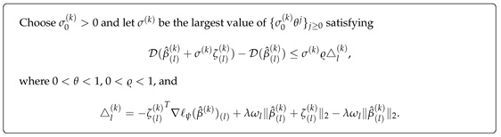
Finally, the update direction is calculated for the gradient of the parameters and the parameters are updated according to a certain step size
The weighted block coordinate gradient descent algorithm is given by Table 1. In general, selecting the tuning parameter using cross-validation method is complicated. As we know from Table 1, the algorithm eliminates the selection process for the tuning parameter . Given an initial value , we can then iterate directly over the until it converges to the range which we expect.
It is worth noting that we have given a direct choice (15) for under a specific weight function given by (14), so the weighted block coordinate gradient descent algorithm will be computationally faster than working iteratively on a fixed grid of tuning parameters (see Meier et al. [12]). If choosing other weight functions, the weighted block coordinate gradient descent algorithm can still be used to solve (6). But then the tuning parameter depends on (unknown), some cross-validation can be used for choosing the parameter .
5. Simulations
In this section, we use simulated datasets to evaluate the performance of the penalized weighted score function estimator. Meier [12] describes block coordinate gradient descent algorithm using the R package grplasso. We modify grplasso, named wgrplasso, and use it to describe the weighted block coordinate gradient descent algorithm. We compare the performance of the wgrplasso algorithm, R package grpreg developed by Breheny [19] and the R package gglasso developed by Yang and Zou [27]. Three main aspects of model performance are considered: correctness of variable selection and accuracy of coefficient estimation, and running time of the algorithm. The evaluation indicators for the model include the following:
- TP: the number of predicted non-zero values in the non-zero coefficient set when determining the model
- TN: the number of predicted zero values in the zero coefficient set when determining the model
- FP: the number of predicted non-zero values in the zero coefficient set when determining the model
- FN: the number of predicted zero values in the non-zero coefficient set when determining the model
- TPR: the ratio of predicted non-zero values in the non-zero coefficient set when determining the model, which is calculated by the following formulation:
- Accur: the ratio of accurate predictions when determining the model, which is calculated by the following formulation:
- Time: the running time of the algorithm.
- BNE: the block norm of the estimation error, which is calculated by the following formulation:
The sample size was 200. We set values of , 600, and 900, and generated 100 random datasets to repeat the simulation. We set to 0.01 and 0.05 and uniformly specify the true non-zero coefficient parameters of the logistic regression models as
For the log odd setting, we consider the following four different models.
(a) In Model I, the observed data X assume sampling from a multivariate normal distribution and the log odd is considered to be the linear case, where the data between groups are independent but the data within groups are correlated. We set the size of each group to 3 and assume that the data within the groups obey , where . Thus, the observed data can then be defined as , where .
(b) In Model II, the observed data X is assumed to be the sum of two uniform distributions and the log odd is considered to be the linear case. Assume that the p-dimensional vectors and W are generated independently and through a uniform distribution of . Thus, the observed data can be defined as .
The log odds for Model I and Model II are then defined as follows
(c) In Model III, the observed data X is assumed to follow a standard multivariate normal distribution and the log ogg is considered to be additive case. Assuming that X obeys the -dimensional standard normal distribution, the observed data can therefore be defined as .
(d) In Model IV, the observed data X is assumed to be the sum of two uniform distributions and the log odd is considered to be the additive case. This means assume that the -dimensional vectors and W are generated independently by a uniform distribution of . Thus, the observed data can be defined as .
The log odds for Model III and Model IV are then defined as follows
Then, the dataset for the response variable Y was generated by the logistic regression models
Table 2 shows the average simulation results of the three algorithms for the linear case, and Figure plots the point-line plots of Model I and Model II for TPR, Accur, Time and MSE.
First, from the TPR perspective, all three algorithms show excellent selection results when the normal distribution assumption is adopted. However, when the uniform distribution assumption is used, the wgrplasso algorithm shows higher correct selection in the nonzero set than the other algorithms, and the wgrplasso algorithm is also more stable in terms of variance.
Second, from the Accur perspective, compared to the gepreg algorithm, the wgrplasso and gglasso algorithms maintain a high selection effect under the assumption of normal distribution. However, Accur is also affected by FP, and the gepreg algorithm and gglasso algorithm are not stable enough to control FP from the perspective of variance. In addition, under the assumption of uniform distribution, both in terms of the effect of selection and the stability of variance, the wgrplasso algorithm has lower control on the FP aspect, which makes the wgrplasso algorithm perform better than the other algorithms in terms of Accur.
Third, from the Time perspective, using the wgrplasso algorithm saves a lot of time, both for the normal distribution assumption and the uniform distribution assumption.
And last, from the BNE perspective, under the assumption of normal distribution, the BNE obtained by wgrplasso and gglasso algorithms are similar and smaller than that obtained by grpreg algorithm. However, under the assumption of uniform distribution, compared with gglasso algorithm and grpreg algorithm, The BNE obtained by wgrplasso algorithm is smaller, which means that wgrplasso algorithm performs better.
Figure 1.
Average TPR, Accur, Time and BNE plots for 100 repetitions of the three algorithms in Model I and Model II.
Figure 1.
Average TPR, Accur, Time and BNE plots for 100 repetitions of the three algorithms in Model I and Model II.
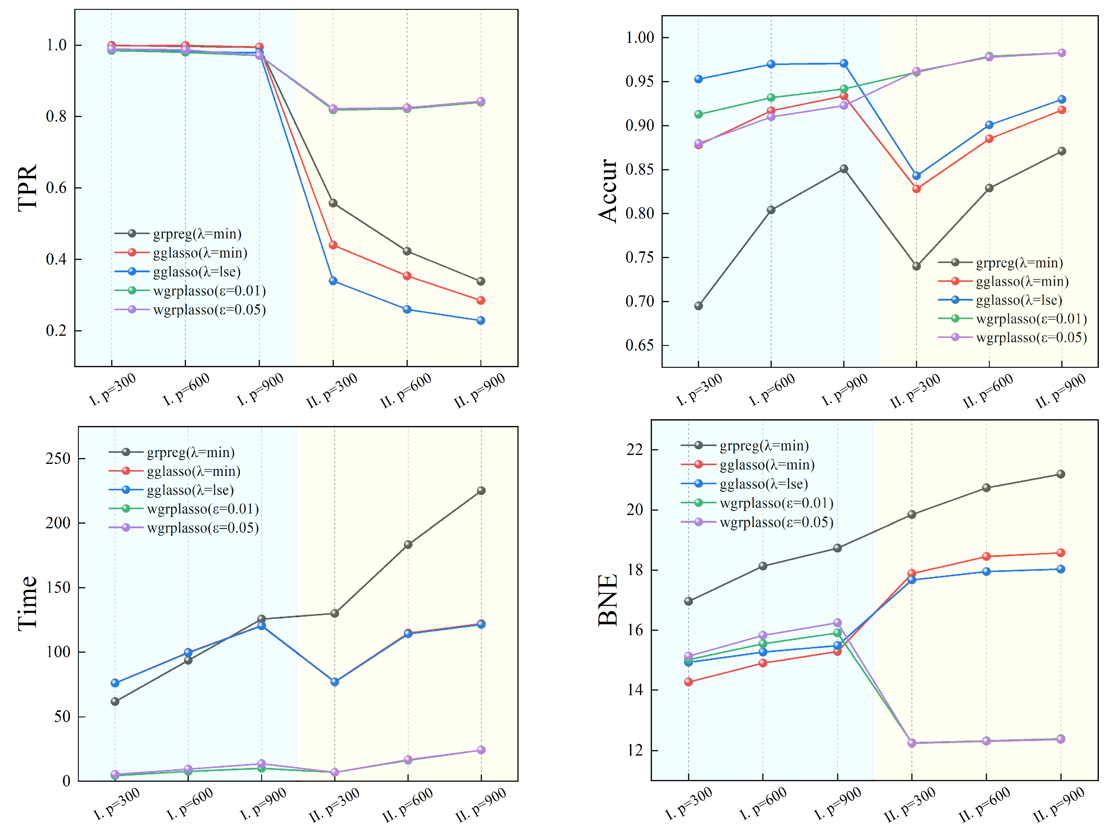
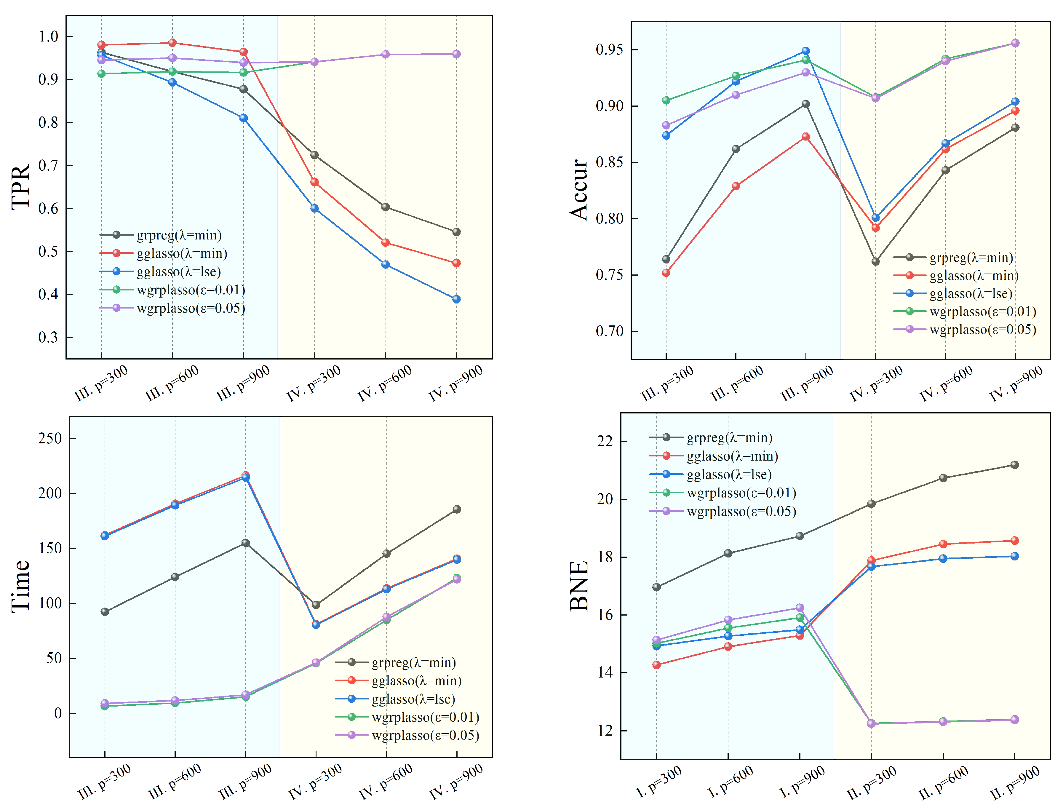
Table 3 gives the simulation results of the three algorithms for the additive case, and Figure plots the point line plots of Models III and IV for TPR, Accur, Time and BNE.
The simulation results show that the grpreg algorithm and the gglasso algorithm in the additive case are reduce both in terms of TPR and Accur, and also show through the variance that the grpreg algorithm and the gglasso algorithm also do not have a stable selection, as well as increasing computational time overhead and BNE. However, wgrplasso obtains similar results in the additive case as in the linear case, and still maintains a better selection. Regardless of TPR, Accur and BNE, the wgrplasso algorithm performs better than the other algorithms, and the advantage in Time is even more obvious.
Figure 2.
Average TPR, Accur, Time and BNE plots for 100 repetitions of the three algorithms in Model III and Model IV.
Figure 2.
Average TPR, Accur, Time and BNE plots for 100 repetitions of the three algorithms in Model III and Model IV.
6. Real data
In this section, we apply our proposed estimates to analyze two real data. The first data comes from the molecular shape and conformation of musk. The second data comes from histologically normal epithelial cells from breast cancer patients and cancer-free prophylactic mastectomy patients. As in the previous section, we set to 0.01 and 0.05, respectively. In Section 6.1 we compare the number of variables selected and the computation time of the three algorithms in the above simulation, and in Section 6.2 we compare the prediction accuracy and the computation time.
6.1. Studies on the molecular structure of Muscadine
The R package of kernlab contains the molecular shape and conformation of musk in the native dataset musk. The data contains a data frame of 476 observations for the following 167 variables. The first 162 of these variables are the distance characteristics of the rays, measured relative to the origin along which each ray is placed. Any experiment with the data should treat these features as being on any continuous scale. Variable 163 is the distance of the oxygen atom to a specified point in 3-space. Variable 164 is the x-displacement from the specified point. Variable 165 is the Y-displacement from the specified point. Variable 166 is the Z displacement from the specified point. The variable 167 tells us that 0 means no musk and 1 means musk.
We used 3/4 of the data for training and performed a third-order B-spline basis function expansion on the training data, and then use the wgrplasso, grpreg, gglasso, and glmnet algorithms for estimation on the expanded training data, respectively. The remaining 1/4 of the data was used as a test, and the estimated coefficients were used to predict the test data, comparing the prediction accuracy, model size, and time for each of the four algorithms. Table 4 gives the experimental results of 100 repetitions.
The experimental results show that wgrplasso has the highest prediction accuracy among the four algorithms, indicating that the algorithm is able to identify the target class more accurately in the task of categorizing musk data, and wgrplasso also exhibits shorter computation time without sacrificing accuracy. This makes the wgrplasso algorithm the preferred algorithm for dealing with the problem of categorizing musk datasets.
6.2. Gene expression studies in epithelial cells of breast cancer patients
We obtained microarray data from the NCBI Gene Expression Omnibus for patient histological epithelial cells. (https://www.ncbi.nlm.nih.gov/geo/) under accession GSE20437. The dataset consists of 42 samples with 22,283 variables. It consists of microarray gene expression data collected from the histologically normal epithelium (NlEpi) from 18 breast cancer patients (HN), 18 undergoing breast reduction (RM) and 6 cancer-free prophylactic mastectomies (PM) in high-risk women. Graham et al. [28] have shown that genes are differentially expressed between HM and RM samples. This is more fully discussed in Yang and Zou [27]. Here, we consider the effect of genes on HM and RM. Similar to Yang and Zou [27] approach to the data, fitting the sparse additive logistic regression model using the Group Lasso penalty while selecting the significant additive components.
As with the setup in Section 6.1, we continue to train with 3/4 of the data and expand the training data using a third-order B-spline basis function and treated them as a group to reflect the role in the additive models, leading to a grouped regression problem with n = 36 and p = 66849. All data were then standardized so that the mean of each original variable was zero and the sample variance was in units. This experiment was repeated 100 times to get the prediction error. We built a complete observational model for the one of experiments, and report the selected genes in wgrplasso, grpreg and gglasso algorithms. These results are listed in Table 5. We observe that the wgrplasso and gglasso algorithms selects more variables than the grpreg algorithm, and wgrplasso has less prediction errors. Summarizing the above results, our proposed penalized weighted score function method can pick much more meaningful variables for explanation and prediction.
7. Conclusion
In our work, we propose the penalized weighted score function method for Group Lasso under logistic regression models. We determine an upper bound on the error of parameter estimation at high probability, and a direct choice of the tuning parameter under a specific weighted function. Under the direct choice of the tuning parameter, we improve the block coordinate descent algorithm to reduce computational time and complexity. Simulation results show that our method not only exhibits better statistical accuracy, but also calculaters faster than competing methods. Indeed, our approach can be extended to other generalized linear models with sparse group structure, which will be a future research.
Appendix
Lemma 1.
(Bach [23]) Consider a three times differentiable convex function such that for all for some Then, for all
Lemma 2.
(Hu et al. [24]) If the inequality holds for all , we have for .
Proof of Lemma 2:
We first introduce the Holder inequality:
Set and . Let and be non-negative real numbers, then
According to the Holder Inequality, set and , we have
becasue , then
here which means . □
Lemma 3.
(Sakhanenko [29]) Let be independent random variables with and for all . Denote and . Then there exists a positive constant A such that for all
Proof of Theorem 1:
Define the event
We state the theorem result on the event A and find an lower bound of .
Define since is the minimizer of , we get
Adding to both sides of (19) are rearranging the inequality, we obtain
According to the fact that is a convex function, by applying Cauchy-Schwarz inequality, it’s Taylor expansion is as follows
Therefore, on the event A we have for .
And then, due to satisfies the condition of three times differentiable, define the function by applying Cauchy-Schwarz inequality, we have
Make , where is a real-valued constant, so is bounded, this means that , by Lemma 1, we have
Further more, combined group restricted eigenvalue condition, we obtain
This implies that
In fact, we can reach the conclusion as follow under all
Therefore, we adopt that meets the above conditions, then we obtain
Based on group restricted eigenvalue condition, choose, for positive constant , substitute into the above equation
Then substitute the equation into (25), we have
Let , we have the following conclusion under the event A
it means that
Now, we prove the probability of event A
take and , it follow that
where . Furthermore, with assumption we obtain
because of
with a positive constant , make have .
Then, and . By lemme 3 we have
Notice for any , we have , then
Our default has which means , and so
Here, we get
As with , we have
which completes the proof of Theorem 1. □
Proof of Theorem 2:
We only need to show that the action of the weight function in the form of (15) as under logistic loss satisfies the assumption (A3)
Denote for , we have
It is not difficult to find that , then
which completes the proof of Theorem 2. □
Funding
The authors’work was supported by Educational Commission of Jiangxi Province of China (No.GJJ160927) and the National Natural Science Foundation of China (No.62266002).
References
- Tibshirani, R. Regression shrinkage and selection via the lasso. Journal of the Royal Statistical Society Series B: Statistical Methodology 1996, 58, 267–288. [Google Scholar] [CrossRef]
- Fan, J.; Li, R. Variable selection via nonconcave penalized likelihood and its oracle properties. Journal of the American statistical Association 2001, 96, 1348–1360. [Google Scholar] [CrossRef]
- Zou, H.; Hastie, T. Regularization and variable selection via the elastic net. Journal of the Royal Statistical Society Series B: Statistical Methodology 2005, 67, 301–320. [Google Scholar] [CrossRef]
- Candes, E.; Tao, T. The Dantzig selector: Statistical estimation when p is much larger than n. The Annals of Statistics 2007, 35, 2313–2351. [Google Scholar]
- Zhang, C.H. Nearly unbiased variable selection under minimax concave penalty. The Annals of Statistics 2010, 38, 894–942. [Google Scholar] [CrossRef] [PubMed]
- Huang, J.; Ma, S.; Zhang, C.H. The iterated lasso for high-dimensional logistic regression. The University of Iowa, Department of Statistics and Actuarial Sciences 2008, 7. [Google Scholar]
- Bianco, A.M.; Boente, G.; Chebi, G. Penalized robust estimators in sparse logistic regression. TEST 2022, 31, 563–594. [Google Scholar] [CrossRef]
- Abramovich, F.; Grinshtein, V. High-dimensional classification by sparse logistic regression. IEEE Transactions on Information Theory 2018, 65, 3068–3079. [Google Scholar] [CrossRef]
- Huang, H.; Gao, Y.; Zhang, H.; Li, B. Weighted Lasso estimates for sparse logistic regression: Non-asymptotic properties with measurement errors. Acta Mathematica Scientia 2021, 41, 207–230. [Google Scholar] [CrossRef]
- Yin, Z. Variable selection for sparse logistic regression. Metrika 2020, 83, 821–836. [Google Scholar] [CrossRef]
- Yuan, M.; Lin, Y. Model selection and estimation in regression with grouped variables. Journal of the Royal Statistical Society Series B: Statistical Methodology 2006, 68, 49–67. [Google Scholar] [CrossRef]
- Meier, L.; Van De Geer, S.; Bühlmann, P. The group lasso for logistic regression. Journal of the Royal Statistical Society Series B: Statistical Methodology 2008, 70, 53–71. [Google Scholar] [CrossRef]
- Wang, L.; You, Y.; Lian, H. Convergence and sparsity of Lasso and group Lasso in high-dimensional generalized linear models. Statistical Papers 2015, 56, 819–828. [Google Scholar] [CrossRef]
- Blazere, M.; Loubes, J.M.; Gamboa, F. Oracle Inequalities for a Group Lasso Procedure Applied to Generalized Linear Models in High Dimension. IEEE Transactions on Information Theory 2014, 60, 2303–2318. [Google Scholar] [CrossRef]
- Kwemou, M. Non-asymptotic oracle inequalities for the Lasso and group Lasso in high dimensional logistic model. ESAIM: Probability and Statistics 2016, 20, 309–331. [Google Scholar] [CrossRef]
- Nowakowski, S.; Pokarowski, P.; Rejchel, W.; Sołtys, A. Improving Group Lasso for high-dimensional categorical data. International Conference on Computational Science. Springer, 2023, pp. 455–470.
- Zhang, Y.; Wei, C.; Liu, X. Group Logistic Regression Models with Lp, q Regularization. Mathematics 2022, 10, 2227. [Google Scholar] [CrossRef]
- Tseng, P. Convergence of a block coordinate descent method for nondifferentiable minimization. Journal of optimization theory and applications 2001, 109, 475–494. [Google Scholar] [CrossRef]
- Breheny, P.; Huang, J. Group descent algorithms for nonconvex penalized linear and logistic regression models with grouped predictors. Statistics and computing 2015, 25, 173–187. [Google Scholar] [CrossRef] [PubMed]
- Belloni, A.; Chernozhukov, V.; Wang, L. Square-root lasso: pivotal recovery of sparse signals via conic programming. Biometrika 2011, 98, 791–806. [Google Scholar] [CrossRef]
- Bunea, F.; Lederer, J.; She, Y. The group square-root lasso: Theoretical properties and fast algorithms. IEEE Transactions on Information Theory 2013, 60, 1313–1325. [Google Scholar] [CrossRef]
- Huang, Y.; Wang, C. Consistent functional methods for logistic regression with errors in covariates. Journal of the American Statistical Association 2001, 96, 1469–1482. [Google Scholar] [CrossRef]
- Bach, F. Self-concordant analysis for logistic regression. Electronic Journal of Statistics 2010, 4, 384–414. [Google Scholar] [CrossRef]
- Hu, Y.; Li, C.; Meng, K.; Qin, J.; Yang, X. Group sparse optimization via lp, q regularization. The Journal of Machine Learning Research 2017, 18, 960–1011. [Google Scholar]
- Bickel, P.J.; Ritov, Y.; Tsybakov, A.B. Simultaneous analysis of Lasso and Dantzig selector. The Annals of Statistics 2009, 37, 1705–1732. [Google Scholar] [CrossRef]
- Tseng, P.; Yun, S. A coordinate gradient descent method for nonsmooth separable minimization. Mathematical Programming 2009, 117, 387–423. [Google Scholar] [CrossRef]
- Yang, Y.; Zou, H. A fast unified algorithm for solving group-lasso penalize learning problems. Statistics and Computing 2015, 25, 1129–1141. [Google Scholar] [CrossRef]
- Graham, K.; de Las Morenas, A.; Tripathi, A.; King, C.; Kavanah, M.; Mendez, J.; Stone, M.; Slama, J.; Miller, M.; Antoine, G.; others. Gene expression in histologically normal epithelium from breast cancer patients and from cancer-free prophylactic mastectomy patients shares a similar profile. British journal of cancer 2010, 102, 1284–1293. [Google Scholar] [CrossRef]
- Sakhanenko, A. Berry-Esseen type estimates for large deviation probabilities. Siberian Mathematical Journal 1991, 32, 647–656. [Google Scholar] [CrossRef]

Table 1.
Weighted block coordinate gradient descent of logistic regression.
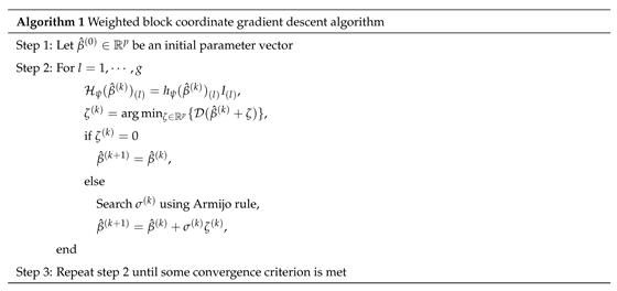
Table 2.
Average results for 100 repetitions of the three algorithms in Model I and Model II.
| Model I | |||||||
| TP | TPR | FP | Accur | Time | BNE | ||
| p=300 | grpreg(=min) | 29.97 (0.30) |
0.999 | 91.71 (20.45) |
0.694 | 75.93 | 16.963 (1.17) |
| gglasso(=min) | 29.94 (0.42) |
0.998 | 36.60 (25.76) |
0.878 | 61.59 | 14.275 (0.55) |
|
| gglasso(=lse) | 29.67 (1.12) |
0.989 | 13.74 (14.25) |
0.953 | 76.11 | 14.933 (0.46) |
|
| wgrplasso(=0.01) | 29.55 (1.08) |
0.985 | 25.80 (8.19) |
0.912 | 4.55 | 15.021 (0.50) |
|
| wgrplasso(=0.05) | 29.67 (0.94) |
0.989 | 25.80 (9.39) |
0.879 | 5.47 | 15.133 (0.56) |
|
| p=600 | grpreg(=min) | 29.91 (0.51) |
0.997 | 115.89 (27.43) |
0.807 | 99.54 | 18.136 (1.49) |
| gglasso(=min) | 29.97 (0.30) |
0.999 | 49.56 (36.29) |
0.917 | 93.64 | 14.904 (0.62) |
|
| gglasso(=lse) | 29.46 (1.43) |
0.982 | 17.25 (18.61) |
0.970 | 99.90 | 15.271 (0.37) |
|
| wgrplasso(=0.01) | 29.40 (1.48) |
0.980 | 40.53 (12.07) |
0.931 | 7.75 | 15.553 (0.52) |
|
| wgrplasso(=0.05) | 29.61 (1.25) |
0.987 | 53.97 (12.85) |
0.909 | 9.42 | 15.829 (0.61) |
|
| p=900 | grpreg(=min) | 29.82 (0.72) |
0.994 | 134.37 (32.87) |
0.851 | 120.47 | 18.736 (1.53) |
| gglasso(=min) | 29.85 (0.66) |
0.995 | 59.19 (42.77) |
0.934 | 125.79 | 15.292 (0.57) |
|
| gglasso(=lse) | 29.37 (1.37) |
0.979 | 25.23 (24.93) |
0.971 | 120.78 | 15.486 (0.41) |
|
| wgrplasso(=0.01) | 29.13 (1.43) |
0.971 | 51.48 (12.94) |
0.942 | 10.06 | 15.907 (0.55) |
|
| wgrplasso(=0.05) | 29.34 (1.32) |
0.978 | 68.55 (14.97) |
0.923 | 13.77 | 16.251 (0.62) |
|
| Model II | |||||||
| TP | TPR | FP | Accur | Time | BNE | ||
| p=300 | grpreg(=min) | 16.74 (4.27) |
0.558 | 65.19 (9.30) |
0.739 | 76.81 | 19.851 (0.82) |
| gglasso(=min) | 13.20 (5.22) |
0.440 | 35.70 (11.74) |
0.825 | 130.13 | 17.889 (0.62) |
|
| gglasso(=lse) | 10.20 (4.78) |
0.340 | 27.69 (11.51) |
0.842 | 77.11 | 17.676 (0.41) |
|
| wgrplasso(=0.01) | 24.57 (2.58) |
0.819 | 6.24 (4.61) |
0.961 | 7.01 | 12.256 (0.54) |
|
| wgrplasso(=0.05) | 24.66 (2.47) |
0.822 | 6.51 (4.75) |
0.961 | 6.95 | 12.241 (0.55) |
|
| p=600 | grpreg(=min) | 12.69 (4.28) |
0.423 | 85.35 (12.24) |
0.829 | 114.24 | 20.737 (0.76) |
| gglasso(=min) | 10.62 (4.09) |
0.354 | 49.77 (14.23) |
0.885 | 183.45 | 18.459 (0.68) |
|
| gglasso(=lse) | 7.80 (4.02) |
0.260 | 37.35 (13.77) |
0.901 | 114.80 | 17.952 (0.44) |
|
| wgrplasso(=0.01) | 24.66 (2.91) |
0.822 | 7.50 (5.40) |
0.979 | 14.17 | 12.323 (0.43) |
|
| wgrplasso(=0.05) | 24.75 (2.81) |
0.825 | 7.71 (5.33) |
0.978 | 15.17 | 12.309 (0.44) |
|
| p=900 | grpreg(=min) | 10.17 (4.53) |
0.339 | 95.97 (14.07) |
0.871 | 141.31 | 21.192 (0.78) |
| gglasso(=min) | 8.55 (4.42) |
0.285 | 52.08 (16.18) |
0.918 | 224.54 | 18.582 (0.73) |
|
| gglasso(=lse) | 6.87 (4.25) |
0.229 | 39.96 (14.36) |
0.930 | 142.08 | 18.038 (0.53) |
|
| wgrplasso(=0.01) | 25.20 (2.70) |
0.840 | 10.77 (6.74) |
0.983 | 22.06 | 12.393 (0.56) |
|
| wgrplasso(=0.05) | 25.29 (2.67) |
0.843 | 11.07 (6.59) |
0.982 | 21.83 | 12.373 (0.58) |
|
Reported numbers are the averages and standard errors (show in parentheses).
Table 3.
Average results for 100 repetitions of the three algorithms in Model III and Model IV.
| Model III | |||||||
| TP | TPR | FP | Accur | Time | BNE | ||
| p=300 | grpreg(=min) | 28.92 (2.15) |
0.964 | 69.87 (20.50) |
0.763 | 161.17 | 18.771 (1.41) |
| gglasso(=min) | 29.43 (3.10) |
0.981 | 74.16 (29.85) |
0.751 | 92.28 | 16.155 (0.84) |
|
| gglasso(=lse) | 28.71 (3.82) |
0.957 | 36.66 (21.05) |
0.874 | 162.14 | 15.849 (0.52) |
|
| wgrplasso(=0.01) | 27.42 (2.86) |
0.914 | 25.95 (7.98) |
0.905 | 6.86 | 15.093 (0.49) |
|
| wgrplasso(=0.05) | 28.38 (2.06) |
0.946 | 33.66 (8.31) |
0.882 | 9.22 | 16.294 (0.55) |
|
| p=600 | grpreg(=min) | 27.57 (4.02) |
0.919 | 80.61 (30.38) |
0.862 | 189.25 | 19.277 (1.56) |
| gglasso(=min) | 29.58 (1.05) |
0.986 | 102.12 (41.15) |
0.829 | 124.10 | 17.521 (1.26) |
|
| gglasso(=lse) | 26.82 (7.21) |
0.894 | 43.86 (34.66) |
0.922 | 190.67 | 16.644 (0.58) |
|
| wgrplasso(=0.01) | 27.57 (2.62) |
0.919 | 41.37 (11.08) |
0.927 | 9.60 | 16.709 (0.60) |
|
| wgrplasso(=0.05) | 28.53 (1.93) |
0.951 | 52.68 (12.12) |
0.910 | 11.95 | 17.024 (0.68) |
|
| p=900 | grpreg(=min) | 26.34 (5.59) |
0.878 | 84.69 (38.07) |
0.902 | 214.50 | 19.459 (1.92) |
| gglasso(=min) | 28.95 (3.20) |
0.965 | 113.34 (49.11) |
0.873 | 155.14 | 17.835 (1.33) |
|
| gglasso(=lse) | 24.33 (9.68) |
0.811 | 39.99 (31.89) |
0.949 | 216.52 | 16.691 (0.46) |
|
| wgrplasso(=0.01) | 27.51 (2.77) |
0.917 | 50.49 (12.26) |
0.941 | 15.23 | 16.939 (0.68) |
|
| wgrplasso(=0.05) | 28.20 (2.33) |
0.940 | 61.77 (12.53) |
0.929 | 16.97 | 17.307 (0.74) |
|
| Model IV | |||||||
| TP | TPR | FP | Accur | Time | BNE | ||
| p=300 | grpreg(=min) | 21.75 (3.94) |
0.725 | 63.24 (9.34) |
0.762 | 80.51 | 23.983 (1.19) |
| gglasso(=min) | 19.86 (4.41) |
0.662 | 52.47 (9.74) |
0.791 | 98.53 | 18.512 (1.21) |
|
| gglasso(=lse) | 18.03 (4.58) |
0.601 | 47.82 (11.15) |
0.801 | 80.87 | 18.051 (1.11) |
|
| wgrplasso(=0.01) | 28.26 (2.05) |
0.942 | 26.31 (8.76) |
0.906 | 45.56 | 14.895 (1.04) |
|
| wgrplasso(=0.05) | 28.26 (2.01) |
0.942 | 26.4 (8.67) |
0.906 | 46.08 | 14.934 (1.03) |
|
| p=600 | grpreg(=min) | 18.12 (4.45) |
0.604 | 82.29 (12.32) |
0.843 | 112.95 | 24.765 (1.38) |
| gglasso(=min) | 15.63 (4.94) |
0.521 | 68.28 (12.20) |
0.862 | 145.22 | 19.121 (1.30) |
|
| gglasso(=lse) | 14.10 (5.07) |
0.470 | 64.11 (13.27) |
0.867 | 113.62 | 18.523 (1.14) |
|
| wgrplasso(=0.01) | 28.77 (1.66) |
0.959 | 34.11 (10.02) |
0.941 | 84.97 | 15.353 (1.11) |
|
| wgrplasso(=0.05) | 28.77 (1.66) |
0.959 | 34.89 (10.25) |
0.940 | 87.64 | 15.38 (1.11) |
|
| p=900 | grpreg(=min) | 16.38 (3.99) |
0.546 | 93.60 (14.46) |
0.881 | 139.78 | 25.239 (1.44) |
| gglasso(=min) | 14.19 (4.69) |
0.473 | 78.21 (13.51) |
0.896 | 185.60 | 19.309 (1.25) |
|
| gglasso(=lse) | 11.67 (4.73) |
0.389 | 67.86 (13.89) |
0.904 | 140.75 | 18.453 (1.09) |
|
| wgrplasso(=0.01) | 28.77 (1.71) |
0.959 | 38.79 (12.26) |
0.956 | 123.20 | 15.780 (1.14) |
|
| wgrplasso(=0.05) | 28.80 (1.71) |
0.960 | 38.79 (11.90) |
0.956 | 121.92 | 15.827 (1.15) |
|
Reported numbers are the averages and standard errors (show in parentheses).
Table 4.
Average prediction accuracy, model size, and time for 100 repetitions of the four algorithms in the musk dataset.
Table 4.
Average prediction accuracy, model size, and time for 100 repetitions of the four algorithms in the musk dataset.
| wgrplasso (ϵ=0.05) |
grpreg (λ=min) |
gglasso (λ=min) |
glmnet (λ=min) |
|
| Prediction accuracy | 0.820 | 0.813 | 0.771 | 0.758 |
| Model size | 66.53 | 31.29 | 30.14 | 53.53 |
| Time | 0.69 | 3.04 | 2.70 | 2.12 |
Table 5.
Average prediction error, model size selected genes for 100 repetitions of three algorithms in microarray gene expression data from histological epithelial cells
Table 5.
Average prediction error, model size selected genes for 100 repetitions of three algorithms in microarray gene expression data from histological epithelial cells
| wgrplasso (ϵ=0.05) |
grpreg (λ=min) |
gglasso (λ=min) |
|
| Prediction error | 0.73 | 0.63 | 0.71 |
| Model size | 14 | 9 | 14 |
| Selected genes | 117_at 1255_g_at 200000_s_at 200002_at 200030_s_at 200040_at 200041_s_at 200655_s_at 200661_at 200729_s_at 201040_at 201465_s_at 202707_at 211997_x_at |
201464_x_at 201465_s_at 201778_s_at 202707_at 204620_s_at 205544_s_at 211997_x_at 213280_at 217921_at |
200047_s_at 200729_s_at 200801_x_at 201465_s_at 202046_s_at 202707_at 205544_s_at 208443_x_at 211374_x_at 211997_x_a212234_at 213280_at 217921_at 220811_at |
Disclaimer/Publisher’s Note: The statements, opinions and data contained in all publications are solely those of the individual author(s) and contributor(s) and not of MDPI and/or the editor(s). MDPI and/or the editor(s) disclaim responsibility for any injury to people or property resulting from any ideas, methods, instructions or products referred to in the content. |
© 2023 by the authors. Licensee MDPI, Basel, Switzerland. This article is an open access article distributed under the terms and conditions of the Creative Commons Attribution (CC BY) license (http://creativecommons.org/licenses/by/4.0/).
Copyright: This open access article is published under a Creative Commons CC BY 4.0 license, which permit the free download, distribution, and reuse, provided that the author and preprint are cited in any reuse.


