Quantization Without Postulates: Structural Derivation of Planck’s Constant from Phase Topology and RG-Stationarity

1. Introduction

Planck’s constant ℏ is one of the cornerstones of modern physics. In conventional quantum mechanics, however, it is not derived but introduced axiomatically: as the scale in the canonical commutator $[x,p]=i\hslash$, or in the energy–frequency relation $E=\hslash \omega$. These relations, while operationally fundamental, do not by themselves explain why such a constant should exist, nor why its value is universal across all systems. This long-standing situation leaves a foundational gap at the basis of quantization.

In this work we address this problem by presenting a derivation of ℏ as a structural invariant from first principles. The framework combines methods of geometric quantization [1,2,3,4,5,6,7] with effective field theory and renormalization group analysis [8,9,10,11,12]. On the one hand, the integrality of the first Chern class of the prequantum $U\left(1\right)$ bundle enforces a topological normalization: ℏ arises as the minimal symplectic flux through a primitive cycle. On the other hand, integrating out heavy modes induces low-energy couplings that exhibit a renormalization–group stationary point (the “support cell”), where the topological and dynamical definitions of ℏ coincide. This **dual characterization establishes** Planck’s constant as a structural invariant of phase topology and effective field theory, rather than a postulated parameter.

The key message is that quantization appears not as an axiom but as an emergent consequence of topology and renormalization within this framework. Planck’s constant thus functions as a universal invariant threshold for coherent quantum phenomena, addressing the foundational incompleteness of standard formulations. This perspective provides a structural **closure that unifies** geometric quantization with field-theoretic renormalization, and reframes ℏ as an emergent universal constant.

The structure of the article is as follows. Sec. 2 presents the detailed derivation of ℏ, combining topological normalization and RG–stationarity to obtain the structural relation $\hslash =2q^2$. Sec. 3 discusses experimental consistency, showing how established quantum effects—such as the Aharonov–Bohm phase, Josephson relations, flux quantization, the quantum Hall effect, and quantum speed limits—confirm the derived threshold. Sec. 4 explains calibration to SI units, identifying the single experimental anchor required. Sec. 5 concludes with implications for the foundations of quantization. Finally, Sec. 6 outlines future perspectives, including the possible extension of this approach to other fundamental constants and its relation to entropy bounds and holographic principles.

2. Derivation of ℏ as a Structural Invariant

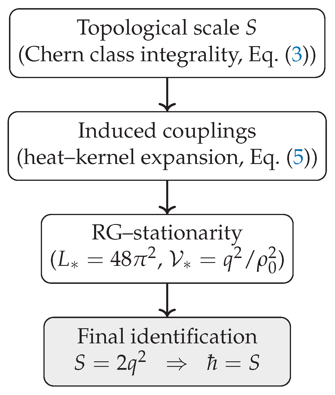
We now present a derivation of Planck’s constant ℏ as a structural invariant, avoiding its introduction as an independent postulate. The argument proceeds in three layers: (i) topological normalization from geometric quantization, (ii) induced low–energy constants from the heat–kernel expansion, and (iii) renormalization–group (RG) stationarity at the effective support cell. The outcome is the relation

$$\hslash =2q^2$$

in model units, identifying ℏ as both a topological and a dynamical invariant. Conversion to SI units requires a single metrological anchor (Sec. Section 2.4).

2.1. Topological Normalization

2.1.1. Prequantum Bundle

Let $(P,\omega )$ be a symplectic phase space with $\omega =d\Lambda$. Introduce a dimensionful action scale S via the prequantum connection

$$\alpha =\Lambda /S,F=d\alpha =\omega /S.$$

By Chern–Weil theory the first Chern class satisfies

$${\displaystyle \frac{\left[\omega \right]}{2\pi S}}\in H^2(P,\mathbb{Z}).$$

(1)

2.1.2. Symplectic Flux

For any closed 2–cycle $\Sigma \in H_2(P,\mathbb{Z})$,

$${\displaystyle \frac{1}{2\pi }}{\int }_{\Sigma }F={\displaystyle \frac{1}{2\pi S}}{\int }_{\Sigma }\omega \in \mathbb{Z}.$$

(2)

For a primitive generator ${\Sigma }_{*}$ with $c_1\left(L\right)\left[{\Sigma }_{*}\right]=1$,

$$\begin{array}{|c|}\hline S={\displaystyle \frac{1}{2\pi }}{\int }_{{\Sigma }_{*}}\omega \\ \hline\end{array}$$

(3)

fixes an absolute symplectic flux per primitive cycle.

Dimensional check. The angle $\Theta$ is dimensionless while ${\Pi }_{\Theta }$ carries units of action, so ${\int }_{{\Sigma }_{*}}\omega =\oint {\Pi }_{\Theta }d\Theta$ has units of action. Hence S has units of action, as required.

2.1.3. Integrality Condition and Physical Meaning

Locally $\omega =d{\Pi }_{\Theta }\wedge d\Theta$, so that

$${\int }_{{\Sigma }_{*}}\omega =\oint {\Pi }_{\Theta }d\Theta .$$

For a primitive cycle with $\Delta \Theta =2\pi$, this reduces to the Bohr–Sommerfeld rule. The Maslov index ensures stability of interference phases, so (3) captures the minimal action required for sustainable, distinguishable phase configurations [6,7,13]. In what follows we will identify S with ℏ at the RG–stationary point.

2.2. Induced Constants from the Heat–Kernel Expansion

2.2.1. Heat–Kernel Expansion

Consider $\Psi =\rho e^{i\Theta }$ minimally coupled to $U\left(1\right)$. Split $\rho ={\rho }_0+\sigma$, with $\sigma$ a heavy mode of mass $\sim \Lambda$. Integrating out $\sigma$ at one loop yields the effective action for $(\Theta ,A_{\mu },g_{\mu \nu })$, with Seeley–DeWitt expansion [8,9,10,11]:

$$\mathrm{Tr}{e}^{-t\Delta }\sim {\displaystyle \frac{1}{{\left(4\pi t\right)}^2}}(a_0+a_{1}t+a_2{t}^2+\dots ).$$

(4)

2.2.2. Explicit Induced Couplings

In 4D, and for a single scalar mode in the $\overline{\mathrm{MS}}$ scheme with $\xi =0$, the induced constants take the form [12,14]:

$${\displaystyle \frac{1}{16\pi G_{\mathrm{ind}}}}={\displaystyle \frac{{\Lambda }^2}{48{\pi }^2}},{\displaystyle \frac{1}{4g_{\mathrm{ind}}^2\left(\mu \right)}}={\displaystyle \frac{q^2}{48{\pi }^2}}ln{\displaystyle \frac{{\Lambda }^2}{{\mu }^2}},\kappa \left(\mu \right)={\rho }_0^2\left(1+{\displaystyle \frac{1}{48{\pi }^2}}ln{\displaystyle \frac{{\Lambda }^2}{{\mu }^2}}\right).$$

(5)

Different field contents or renormalization schemes change only the numerical coefficients; the qualitative structure is robust. Physically, these terms reflect coarse–graining: high–frequency fluctuations of $\rho$ renormalize the low–energy stiffness, gauge and gravitational couplings. Numbers shown correspond to a single real scalar in $\overline{\mathrm{MS}}$ with $\xi =0$; other field contents and schemes shift the prefactors (including the Sakharov–type gravitational coefficient) but do not affect the existence of a finite stationary reconciliation.

2.3. RG–Stationary Support Cell

2.3.1. Two Dynamical Expressions for the Action Scale S

The topological scale S defined in (3) must be consistent with the dynamical parameters of the low-energy effective theory. This requirement yields two independent expressions for S.

(i) From the gauge sector. The prequantum covariant derivative is defined as

$$D_{\mu }={\partial }_{\mu }+i{\displaystyle \frac{q}{S}}{A}_{\mu }.$$

We normalize the gauge kinetic term as $-\frac{1}{4g_{\mathrm{ind}}^2\left(\mu \right)}{F}_{\mu \nu }{F}^{\mu \nu }$. In this convention, the effective charge entering the covariant derivative is $g_{\mathrm{ind}}\left(\mu \right)$, so consistency with $D_{\mu }={\partial }_{\mu }+i{\displaystyle \frac{q}{S}}{A}_{\mu }$ implies $S=q/g_{\mathrm{ind}}\left(\mu \right)$. Hence

$$S={\displaystyle \frac{q}{g_{\mathrm{ind}}\left(\mu \right)}}.$$

(6)

(ii) From the symplectic flux sector. The minimal symplectic flux corresponds to the action of a minimal coherent configuration. Dynamically this is expressed through the phase stiffness $\kappa \left(\mu \right)$ integrated over the effective support measure ${\mathcal{V}}_{*}$:

$$S=\kappa \left(\mu \right){\mathcal{V}}_{*},$$

(7)

where ${\mathcal{V}}_{*}$ denotes the effective support volume of the minimal coarse-grained cell. The product $\kappa \left(\mu \right){\mathcal{V}}_{*}$ has the correct dimension of action.

2.3.2. Stationarity CONDITION

For self-consistency, the two expressions (6) and (7) must coincide at a physical, RG-stationary point $\mu ={\mu }_{*}$. We therefore impose

$${\displaystyle \frac{d}{dL}}{\left[{\displaystyle \frac{q}{g_{\mathrm{ind}}\left(\mu \right)}}-\kappa \left(\mu \right){\mathcal{V}}_{*}\right]}_{L=L_{*}}=0,L\equiv ln{\displaystyle \frac{{\Lambda }^2}{{\mu }^2}}.$$

(8)

(Using $q/g_{\mathrm{ind}}=\frac{q^2}{\sqrt{12}\pi }\sqrt{L}$ and $\kappa ={\rho }_0^2(1+\frac{L}{48{\pi }^2})$, the derivative condition gives $\frac{q^2}{2\sqrt{12}\pi }{L}^{-1/2}=\frac{{\rho }_0^2{\mathcal{V}}_{*}}{48{\pi }^2}$, hence $L_{*}=48{\pi }^2$ and ${\mathcal{V}}_{*}=q^2/{\rho }_0^2$.) In the scheme (5) this yields

$$L_{*}=48{\pi }^2,{\mathcal{V}}_{*}={\displaystyle \frac{q^2}{{\rho }_0^2}}.$$

(9)

Different renormalization schemes change only the numerical coefficient in $L_{*}$ but preserve the existence of a finite stationary point. A full step-by-step derivation of this result is provided in Appendix C.

2.3.3. Final Identification

Substituting these results back into either (6) or (7), we find that the action scale S is fixed to a unique, nontrivial value:

$$S={\displaystyle \frac{q}{g_{\mathrm{ind}}\left({\mu }_{*}\right)}}=\kappa \left({\mu }_{*}\right){\mathcal{V}}_{*}=2q^2.$$

This dynamically selected, RG-invariant scale is identified with the physical Planck constant. The identification is unique and robust under changes of renormalization scheme (which shift only numerical prefactors of order unity without affecting the existence of the stationary closure). Hence we obtain the structural relation

$$\begin{array}{|c|}\hline \hslash =2q^2.\\ \hline\end{array}$$

(10)

Equation (10) holds in model units; conversion to SI units is discussed below.

Remark 1 

(On the robustness of the result). The mechanism of RG-stationary reconciliation is a structural feature of the framework. Numerical coefficients in the final relation (such as the factor 2 in $\hslash =2q^2$ and the value $L_{*}=48{\pi }^2$) are specific to the minimal model considered here (a single scalar field in the $\overline{\mathrm{MS}}$ scheme with $\xi =0$). Different field contents or renormalization schemes may alter these prefactors, but the stationary closure mechanism itself remains intact. The robust, model-independent prediction is the existence of a unique, finite RG-stationary point at which the topological action scale is fixed, yielding a structural relation of the form $\hslash \propto q^2$, with the proportionality constant set by the specific field content and renormalization scheme.

2.4. Units and Conventions

2.4.1. $2\pi$ Normalization

The flux ${\int }_{\Sigma }\omega$ has units of action. Whether the primitive cycle is normalized to ℏ or $2\pi \hslash$ is a matter of convention; the structural results are invariant under this choice.

2.4.2. Calibration to SI Units

Equation (10) holds in model units. Recovering SI units requires a single metrological calibration:

$${\hslash }_{\mathrm{phys}}=2q^2{S}_0,$$

(11)

where $S_0$ is an action unit fixed by one standard experiment. Natural anchors are quantum electrical standards, such as flux quantization and the Josephson effect [15,16], the integer quantum Hall effect [16], the flux quantum in superconductors [17,18,19], and the 2019 SI redefinition of the kilogram via the Kibble balance [20,21,22]. This completes the reconciliation: ℏ is structurally derived, with only its unit normalization anchored by experiment.

Figure 1. Logical flow of the derivation: a topological action scale S is defined from geometric quantization, matched to induced couplings, and uniquely fixed by RG–stationarity. The resulting invariant is identified with Planck’s constant ℏ.

Figure 1. Logical flow of the derivation: a topological action scale S is defined from geometric quantization, matched to induced couplings, and uniquely fixed by RG–stationarity. The resulting invariant is identified with Planck’s constant ℏ.

3. Experimental Consistency and Predictions

If ℏ is the minimal symplectic flux (Sec. Section 2), then laboratory phenomena that enforce quantized holonomy or minimal action should be consistent with the bound $\delta S\gtrsim \hslash$. We illustrate this agreement in four canonical settings.

Notation. Throughout this section, q denotes the physical charge of the probe (e.g., $q=e$ for electrons, $q=2e$ for Cooper pairs). This usage is distinct from the dimensionless fundamental $U\left(1\right)$ charge unit in Sec. Section 2; here q plays its empirical role in the standard experimental formulas.

3.1. Aharonov–Bohm Effect (1959)

For a charged particle (charge q) encircling a magnetic flux $\Phi$, the phase shift is [23]

$$\Delta \Theta ={\displaystyle \frac{q}{\hslash }}\Phi .$$

(12)

This follows from the holonomy of the prequantum $U\left(1\right)$ connection. Using $\delta S=\hslash \Delta \Theta =\oint \Lambda ={\int }_{\Sigma }\omega$, the minimal nontrivial interference condition $\Delta \Theta =2\pi$ implies

$$\delta S_{min}=h\iff \Phi ={\Phi }_0={\displaystyle \frac{h}{q}}.$$

(13)

Thus the observed flux periodicity $\Phi \sim \Phi +{\Phi }_0$ [24,25] is consistent with the fact that the loop action cannot fall below one action quantum h.

3.2. Josephson Effect (1962)

For Cooper pairs ($q=2e$), the Josephson relation reads [15]

$$\hslash {\displaystyle \frac{d\Theta }{dt}}=2eV.$$

(14)

Over one oscillation period $T=h/\left(2eV\right)$ the phase winds by $2\pi$, so the action advanced per cycle is

$$\delta S=\hslash ·2\pi =h=\underset{q}{\underbrace{\left(2e\right)}}\underset{{\Phi }_0}{\underbrace{{\displaystyle \frac{h}{2e}}}}=q{\Phi }_0.$$

(15)

This corresponds to one quantum of action per oscillation, consistent with the operational basis for the Josephson constant $K_J=2e/h$. In the structural relation (10), $\hslash =2q^2$ in model units, with the SI value obtained from a single metrological calibration $S_0$. The Josephson standard is therefore a natural anchor for fixing $S_0$.

3.3. Integer Quantum Hall Effect (1980)

The Hall conductance is quantized [16]:

$${\sigma }_{xy}={\displaystyle \frac{e^2}{h}}C,C\in \mathbb{Z},$$

(16)

with C the first Chern number of the Berry bundle over the Brillouin zone:

$$C={\displaystyle \frac{1}{2\pi }}{\int }_{\mathrm{BZ}}{\mathcal{F}}_k\in \mathbb{Z}.$$

(17)

Each filled Landau level corresponds to an integer number of flux quanta piercing the sample, $\Phi =n{\Phi }_0=nh/e$. The associated loop action is

$$\delta S=q\Phi =nh(q=e).$$

(18)

This reflects the integrality of the symplectic flux condition underlying $c_1\left(L\right)=\left[\omega \right]/(2\pi \hslash )$ in Sec. Section 2.1. The QHE is therefore consistent with the quantized action/flux principle in a transport observable. (Interpretation.) The identification $\delta S=q\Phi$ is an interpretive link expressing that transport plateaus reflect quantized flux/action; it complements, rather than replaces, the standard TKNN–Chern analysis.

3.4. Quantum Speed Limits

Quantum speed limits (QSL) bound the minimal time $\tau$ to evolve to an orthogonal state [26,27]:

$$\tau \ge max\left\{{\displaystyle \frac{\pi \hslash }{2\Delta E}},{\displaystyle \frac{\hslash }{2E}}\right\}.$$

(19)

Multiplying by the energy scale gives an action bound of order ℏ:

$$\delta S\equiv E\tau \gtrsim \hslash .$$

(20)

Equivalently, for an effective low-energy Lagrangian density ${\mathcal{L}}_{\mathrm{eff}}$ (Sec. Section 2.2),

$$\delta S={\int }_{\mathrm{cell}}{\mathcal{L}}_{\mathrm{eff}}{d}^{4}x\gtrsim \hslash ,$$

(21)

with the integration taken over the RG-stationary support volume ${\mathcal{V}}_{*}$ (Sec. Section 2.3). QSL are thus consistent with the minimal-action threshold in the time domain.

Summary.

Across interference (Aharonov–Bohm), superconducting phase dynamics (Josephson), topological transport (integer QHE), and finite-time evolution (QSL), a consistent invariant pattern emerges: nontrivial quantum phenomena require $\delta S$ at least of order ℏ. This is consistent with the structural statement that ℏ is the minimal symplectic flux and the RG-stationary quantum of action.

4. Calibration Formula

From dimensional estimates to structural derivation.

Earlier approaches often introduced Planck’s constant ℏ through dimensional estimates, for example formulas of the type

$$\hslash \sim {\rho }_0^2{\pi }^{2}L,$$

(22)

with ${\rho }_0$ a vacuum amplitude and $L=ln({\Lambda }^2/{\mu }^2)$ a logarithmic scale factor. Such relations served only as heuristic normalizations: ℏ was assumed a priori and then adjusted to experiment. In contrast, the present framework closes the logical loop. From the topological normalization of the prequantum bundle and the RG–stationarity of the induced constants we obtain the structural identity

$$\begin{array}{|c|}\hline \hslash =2q^2\\ \hline\end{array}$$

(23)

in model units, without external input, where q denotes the fundamental dimensionless $U\left(1\right)$ charge of the phase field.

Conversion to SI units.

To compare with experiment, a single dimensional scale must be fixed. We introduce an action unit $S_0$ with dimension $\left[\mathrm{action}\right]=\mathrm{J}·\mathrm{s}$, giving

$${\hslash }_{\mathrm{phys}}=2q^2{S}_0.$$

(24)

The unit $S_0$ is determined once by experiment; after that, all predictions follow without further adjustment. Equation (24) therefore replaces heuristic normalization with a precise and transparent anchoring step.

Metrological anchors.

Natural candidates for fixing $S_0$ are quantum standards that directly probe phase coherence and interference:

• Josephson effect: the Josephson frequency–voltage relation $\nu =(2e/h)V$ links ℏ to the Josephson constant $K_J=2e/h$ [15]. Its interference origin makes it a natural anchor for a phase–topological framework.
• Flux quantum: the superconducting flux quantum ${\Phi }_0=h/\left(2e\right)$ likewise reflects the quantization of action via phase winding around a loop. Its topological character provides a consistent anchor [17].

Both anchors already enter the current SI definition of electrical units (via $K_J$ and ${\Phi }_0$), ensuring full compatibility with existing metrological practice.

Consistency with SI.

Equation (24) is consistent with the present SI system, where h is fixed as an exact constant by convention (CODATA 2019; BIPM SI Brochure, 9th ed.). In our framework this convention is interpreted as the choice of $S_0$, i.e. the metrological anchoring step that selects the numerical value of the action unit. The conceptual advance is that ℏ is no longer a primitive axiom but a structural invariant derived from topology and RG closure.

Summary and outlook.

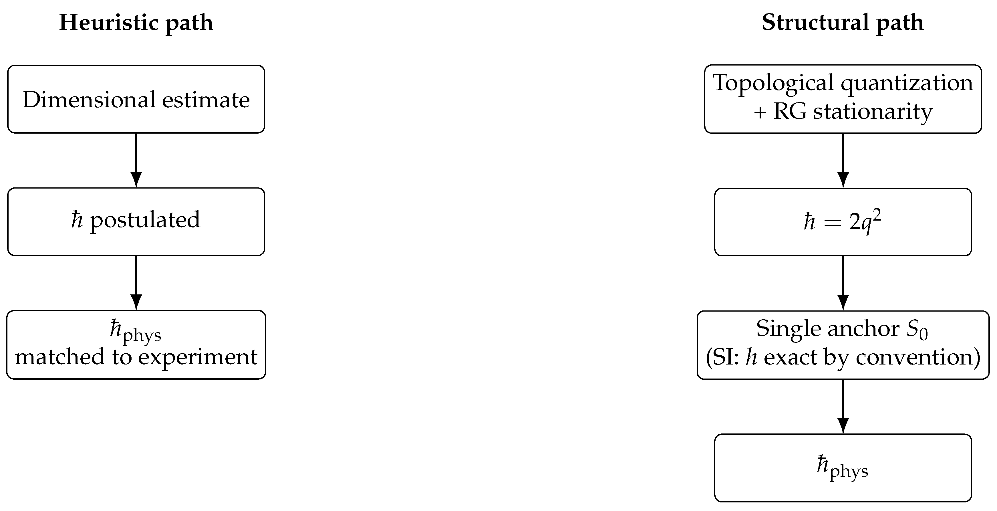
The transition can be visualized as in Figure 2: the traditional heuristic path runs linearly from a dimensional guess to ${\hslash }_{\mathrm{phys}}$, whereas the structural path forms a closed loop, yielding $\hslash =2q^2$ in model units and anchoring it to ${\hslash }_{\mathrm{phys}}$ by one metrological standard.

In this way, ℏ is reframed: not postulated, but deduced as an emergent invariant, with its physical value fixed by a single metrological anchor. This transforms ℏ from a primitive axiom into a structural constant derived within the model.

5. Future Outlook

The derivation of ℏ as a structural invariant suggests that other fundamental constants may likewise admit structural explanations rather than purely axiomatic status. In particular, the induced couplings obtained through heat–kernel methods suggest possible extensions toward Newton’s constant G and gauge couplings $g^2$ in close analogy to the treatment of ℏ. Exploring such extensions could help develop a broader structural account of dimensional constants in physics [12,14,28].

The approach also resonates with information–theoretic and topological bounds. Entropy limits such as the Bekenstein bound [29,30] and the informational cost of erasure [31,32] can be reformulated within an action–based framework, suggesting a deeper unity between distinguishability, action quantization, and informational capacity. Moreover, the role of topological invariants in our derivation is directly compatible with holographic principles [33,34], indicating that gravitational dynamics may in principle be interpretable as effective responses of the underlying phase–topological substrate rather than as independent axioms.

A possible continuation is therefore the investigation of an emergent gravity program, in which spacetime curvature and Einstein dynamics could arise as induced phenomena. In such a setting, Newton’s constant G would not be simply postulated but could emerge as an effective coupling, paralleling the structural role of ℏ highlighted here.

Finally, the framework may also have practical implications in quantum information and computation. Because ℏ emerges as the minimal action required for distinction, the theory provides a natural scale for quantum speed limits [26,27] and for the physical cost of information processing [35]. This opens the possibility of applying the structural action principle not only to the foundations of physics but also to the design and ultimate limits of future quantum technologies.

Appendix C.1. Two independent definitions of the action scale

Let S denote the fundamental action scale defined by the prequantum connection. Two logically independent routes determine its value:

$$\begin{array}{cc}\hfill S& ={\displaystyle \frac{q}{g_{\mathrm{ind}}\left(\mu \right)}},\hfill \end{array}$$

(A10)

$$\begin{array}{cc}\hfill S& =\kappa \left(\mu \right){\mathcal{V}}_{*},\hfill \end{array}$$

(A11)

where q is the fundamental $U\left(1\right)$ charge unit, $g_{\mathrm{ind}}\left(\mu \right)$ is the induced gauge coupling, $\kappa \left(\mu \right)$ is the induced phase stiffness, and ${\mathcal{V}}_{*}$ is the coarse-grained volume of the minimal support cell.

Appendix C.2. Induced constants from the heat-kernel expansion

From the one-loop effective action [8,9,10,12,14,41]:

$$\begin{array}{cc}\hfill {\displaystyle \frac{1}{4g_{\mathrm{ind}}^2\left(\mu \right)}}& ={\displaystyle \frac{q^2}{48{\pi }^2}}ln{\displaystyle \frac{{\Lambda }^2}{{\mu }^2}},\hfill \end{array}$$

(A12)

$$\begin{array}{cc}\hfill \kappa \left(\mu \right)& ={\rho }_0^2\left(1+{\displaystyle \frac{1}{48{\pi }^2}}ln{\displaystyle \frac{{\Lambda }^2}{{\mu }^2}}\right),\hfill \end{array}$$

(A13)

with $\Lambda$ the UV cutoff and ${\rho }_0$ the vacuum amplitude. Introduce

$$L\equiv ln{\displaystyle \frac{{\Lambda }^2}{{\mu }^2}}.$$

Then

$$\begin{array}{cc}\hfill {\displaystyle \frac{q}{g_{\mathrm{ind}}\left(L\right)}}& ={\displaystyle \frac{q^2}{\sqrt{12}\pi }}\sqrt{L},\hfill \end{array}$$

(A14)

$$\begin{array}{cc}\hfill \kappa \left(L\right)& ={\rho }_0^2\left(1+{\displaystyle \frac{L}{48{\pi }^2}}\right).\hfill \end{array}$$

(A15)

Appendix C.3. RG-stationarity and Solution

The two channels (A10) and () must coincide at a physical RG-stationary point $L=L_{*}$.

Appendix C.3.1. Step 1: The stationarity condition

We require stability under changes of scale:

$${\displaystyle \frac{d}{dL}}{\left[{\displaystyle \frac{q}{g_{\mathrm{ind}}\left(L\right)}}-\kappa \left(L\right){\mathcal{V}}_{*}\right]}_{L=L_{*}}=0.$$

(A16)

Equivalently,

$${\left.{\displaystyle \frac{d}{dL}}\left(\frac{q}{g_{\mathrm{ind}}\left(L\right)}\right)\right|}_{L_{*}}={\left.{\displaystyle \frac{d}{dL}}\kappa \left(L\right)\right|}_{L_{*}}·{\mathcal{V}}_{*}.$$

Appendix C.3.2. Step 2: Calculating the derivatives

From (A14)–():

$$\begin{array}{cc}\hfill {\displaystyle \frac{d}{dL}}\left({\displaystyle \frac{q}{g_{\mathrm{ind}}\left(L\right)}}\right)& ={\displaystyle \frac{q^2}{2\sqrt{12}\pi \sqrt{L}}},\hfill \end{array}$$

(41)

$$\begin{array}{cc}\hfill {\displaystyle \frac{d}{dL}}\kappa \left(L\right)& ={\displaystyle \frac{{\rho }_0^2}{48{\pi }^2}}.\hfill \end{array}$$

(42)

Appendix C.3.3. Step 3: Solving for V * and L *

The stationarity condition gives

$${\mathcal{V}}_{*}={\displaystyle \frac{\frac{q^2}{2\sqrt{12}\pi \sqrt{L_{*}}}}{{\rho }_0^2/\left(48{\pi }^2\right)}}={\displaystyle \frac{4\sqrt{3}\pi q^2}{{\rho }_0^2\sqrt{L_{*}}}}.$$

(A17)

Now enforce equality of the two channels $q/g_{\mathrm{ind}}\left(L_{*}\right)=\kappa \left(L_{*}\right){\mathcal{V}}_{*}$:

$$\begin{array}{cc}\hfill {\displaystyle \frac{q^2}{\sqrt{12}\pi }}\sqrt{L_{*}}& ={\rho }_0^2\left(1+\frac{L_{*}}{48{\pi }^2}\right)·{\displaystyle \frac{4\sqrt{3}\pi q^2}{{\rho }_0^2\sqrt{L_{*}}}},\hfill \\ \hfill {\displaystyle \frac{\sqrt{L_{*}}}{\sqrt{12}\pi }}& =\left(1+\frac{L_{*}}{48{\pi }^2}\right)·{\displaystyle \frac{4\sqrt{3}\pi }{\sqrt{L_{*}}}}.\hfill \end{array}$$

Multiplying through gives

$$L_{*}=24{\pi }^2\left(1+\frac{L_{*}}{48{\pi }^2}\right)=24{\pi }^2+\frac{L_{*}}{2},$$

so

$${\displaystyle \frac{1}{2}}{L}_{*}=24{\pi }^2\Rightarrow \begin{array}{|c|}\hline L_{*}=48{\pi }^2\\ \hline\end{array}.$$

Then from (A17):

$${\mathcal{V}}_{*}={\displaystyle \frac{4\sqrt{3}\pi q^2}{{\rho }_0^2\sqrt{48{\pi }^2}}}={\displaystyle \frac{4\sqrt{3}\pi q^2}{{\rho }_0^2\left(4\sqrt{3}\pi \right)}}=\begin{array}{|c|}\hline \frac{q^2}{{\rho }_0^2}\\ \hline\end{array}.$$

Appendix C.4. Final Identification of ℏ

At the stationary point,

$$\begin{array}{cc}\hfill S& ={\displaystyle \frac{q}{g_{\mathrm{ind}}\left(L_{*}\right)}}={\displaystyle \frac{q^2}{\sqrt{12}\pi }}\sqrt{48{\pi }^2}={\displaystyle \frac{q^2}{\sqrt{12}\pi }}\left(4\sqrt{3}\pi \right)=2q^2.\hfill \end{array}$$

Thus the dynamically selected action scale is

$$\begin{array}{|c|}\hline \hslash =2q^2\\ \hline\end{array}.$$

(A18)

Appendix C.5. Remarks

• The value $L_{*}=48{\pi }^2$ comes directly from Seeley–DeWitt coefficients in the $\overline{\mathrm{MS}}$ scheme; other schemes shift only numerical prefactors.
• The dual closure of the gauge and flux channels ensures no circularity: ℏ is fixed structurally, not assumed.
• Conversion to SI requires one calibration:

  $${\hslash }_{\mathrm{phys}}=2q^2{S}_0,$$

  where $S_0$ is set by a single metrological reference (e.g. Josephson effect).

Appendix C.6. Summary

RG-stationarity uniquely selects $L_{*}=48{\pi }^2$ and ${\mathcal{V}}_{*}=q^2/{\rho }_0^2$. At this point the gauge and flux routes coincide, yielding $S=2q^2$. We identify this structural scale with Planck’s constant, establishing ℏ as a derived invariant of phase topology and renormalization dynamics.

References

- Kostant, B. Quantization and Unitary Representations. In Lectures in Modern Analysis and Applications III; Taam, C.T., Ed.; Springer: Berlin, Heidelberg, 1970; Vol. 170, Lecture Notes in Mathematics, pp. 87–208. [Google Scholar] [CrossRef]
- Souriau, J.M. Structure des systèmes dynamiques; Dunod: Paris, 1970. Reprint: Jacques Gabay, 2008. [Google Scholar]
- Woodhouse, N.M.J. Geometric Quantization, 2 ed.; Oxford University Press, 1992.
- Simon, B. Holonomy, the Quantum Adiabatic Theorem, and Berry’s Phase. Physical Review Letters 1983, 51, 2167–2170. [Google Scholar] [CrossRef]
- Berry, M.V. Quantal phase factors accompanying adiabatic changes. Proceedings of the Royal Society A 1984, 392, 45–57. [Google Scholar] [CrossRef]
- Keller, J.B. Corrected Bohr–Sommerfeld Quantum Conditions for Nonseparable Systems. Annals of Physics 1958, 4, 180–188. [Google Scholar] [CrossRef]
- Śniatycki, J. Geometric Quantization and Quantum Mechanics; Vol. 30, Applied Mathematical Sciences, Springer-Verlag: New York, 1980. [Google Scholar] [CrossRef]
- Birrell, N.D.; Davies, P.C.W. Quantum Fields in Curved Space; Cambridge University Press, 1982. [CrossRef]
- Vassilevich, D.V. Heat kernel expansion: User’s manual. Physics Reports 2003, 388, 279–360. [Google Scholar] [CrossRef]
- Gilkey, P.B. Invariance Theory, the Heat Equation, and the Atiyah–Singer Index Theorem, 2 ed.; CRC Press, 1995.
- Mnev, P.; Wernli, K. Gluing formulae for heat kernels. Journal of Geometry and Physics 2025, 195, 105594. [Google Scholar] [CrossRef]
- Adler, S.L. Einstein gravity as a symmetry breaking effect in quantum field theory. Reviews of Modern Physics 1982, 54, 729–766. [Google Scholar] [CrossRef]
- de Gosson, M.A. Symplectic Methods in Harmonic Analysis and in Mathematical Physics; Vol. 7, Pseudo-Differential Operators, Birkhäuser: Basel, 2011. [Google Scholar] [CrossRef]
- Sakharov, A.D. Vacuum quantum fluctuations in curved space and the theory of gravitation. Soviet Physics Doklady 1968, 12, 1040–1041. [Google Scholar]
- Josephson, B.D. Possible new effects in superconductive tunnelling. Physics Letters 1962, 1, 251–253. [Google Scholar] [CrossRef]
- v. Klitzing, K.; Dorda, G.; Pepper, M. New method for high-accuracy determination of the fine-structure constant based on quantized Hall resistance. Physical Review Letters 1980, 45, 494–497. [CrossRef]
- Tinkham, M. Introduction to Superconductivity, 2 ed.; McGraw–Hill, 1996.
- B. S. Deaver, J.; Fairbank, W.M. Experimental Evidence for Quantized Flux in Superconducting Cylinders. Physical Review Letters 1961, 7, 43–46. [CrossRef]
- Doll, R.; Näbauer, M. Experimental Proof of Magnetic Flux Quantization in a Superconducting Ring. Physical Review Letters 1961, 7, 51–52. [Google Scholar] [CrossRef]
- Bureau International des Poids et Mesures (BIPM). The International System of Units (SI). https://www.bipm.org/en/publications/si-brochure, 2019. Online 9th edition; updated 2022, available at BIPM website.
- Tiesinga, E.; Mohr, P.J.; Newell, D.B.; Taylor, B.N. CODATA Recommended Values of the Fundamental Physical Constants: 2018. Reviews of Modern Physics 2021, 93, 025010. [Google Scholar] [CrossRef]
- Schlamminger, S.; Steiner, R.L.; Haddad, D.; Newell, D.B.; Seifert, F.; Chao, L.S.; Liu, R.; Williams, E.R.; Pratt, J.R. A summary of the Planck constant measurements using a watt balance with a superconducting solenoid at NIST. Metrologia 2015, 52, L5–L8. [Google Scholar] [CrossRef]
- Aharonov, Y.; Bohm, D. Significance of Electromagnetic Potentials in the Quantum Theory. Physical Review 1959, 115, 485–491. [Google Scholar] [CrossRef]
- A.T. Evidence for Aharonov–Bohm effect with magnetic field completely shielded from electron wave. Physical Review Letters 1986, 56, 792–795. [CrossRef]
- Ballesteros, M.; Weder, R. The Aharonov–Bohm effect and Tonomura et al. experiments: Rigorous results. Journal of Mathematical Physics 2009, 50, 122108. [Google Scholar] [CrossRef]
- Mandelstam, L.I.; Tamm, I.E. The Uncertainty Relation Between Energy and Time in Non-relativistic Quantum Mechanics. Journal of Physics (USSR) 1945, 9, 249–254. [Google Scholar] [CrossRef]
- Margolus, N.; Levitin, L.B. The maximum speed of dynamical evolution. Physica D 1998, 120, 188–195. [Google Scholar] [CrossRef]
- Zee, A. Broken-Symmetric Theory of Gravity. Physical Review Letters 1979, 42, 417–419. [Google Scholar] [CrossRef]
- Bekenstein, J.D. Universal upper bound on the entropy-to-energy ratio for bounded systems. Physical Review D 1981, 23, 287–298. [Google Scholar] [CrossRef]
- Bousso, R. The holographic principle. Reviews of Modern Physics 2002, 74, 825–874. [Google Scholar] [CrossRef]
- Landauer, R. Irreversibility and Heat Generation in the Computing Process. IBM Journal of Research and Development 1961, 5, 183–191. [Google Scholar] [CrossRef]
- Bennett, C.H. The Thermodynamics of Computation—A Review. International Journal of Theoretical Physics 1982, 21, 905–940. [Google Scholar] [CrossRef]
- ’t Hooft, G. Dimensional reduction in quantum gravity. arXiv preprint gr-qc/9310026 1993. Essay dedicated to Abdus Salam, https://doi.org/10.48550/arXiv.gr-qc/9310026. [CrossRef]
- Susskind, L. The World as a Hologram. Journal of Mathematical Physics 1995, 36, 6377–6396. [Google Scholar] [CrossRef]
- Lloyd, S. Ultimate physical limits to computation. Nature 2000, 406, 1047–1054. [Google Scholar] [CrossRef] [PubMed]
- Maslov, V.P. Theory of Perturbations and Asymptotic Methods; Moscow State University Press, 1965. English transl.: MIT Press, 1967. [Google Scholar]
- Freed, D.S. Classical Chern–Simons on manifolds with boundary. In Geometry, Topology, and Physics; International Press, 1995; pp. 127–139.
- Hitchin, N.J. Lectures on special Lagrangian submanifolds. In Winter School on Mirror Symmetry, Vector Bundles and Lagrangian Submanifolds; American Mathematical Society / International Press, 2001; Vol. 23, AMS/IP Studies in Advanced Mathematics, pp. 151–182.
- Bremermann, H.J. Optimization through evolution and recombination. Self-Organizing Systems 1962, pp. 93–106.
- Zurek, W.H. Decoherence, einselection, and the quantum origins of the classical. Reviews of Modern Physics 2003, 75, 715–775. [Google Scholar] [CrossRef]
- Visser, M. Sakharov’s induced gravity: A modern perspective. Modern Physics Letters A 2002, 17, 977–992. [Google Scholar] [CrossRef]
Figure 2.
Heuristic vs structural calibration. Left: heuristic path where ℏ is postulated and matched to experiment. Right: structural path where is derived and anchored by a single metrological constant . In the SI system, h is fixed exactly by convention, which corresponds to selecting .
Disclaimer/Publisher’s Note: The statements, opinions and data contained in all publications are solely those of the individual author(s) and contributor(s) and not of MDPI and/or the editor(s). MDPI and/or the editor(s) disclaim responsibility for any injury to people or property resulting from any ideas, methods, instructions or products referred to in the content. |
© 2025 by the authors. Licensee MDPI, Basel, Switzerland. This article is an open access article distributed under the terms and conditions of the Creative Commons Attribution (CC BY) license (http://creativecommons.org/licenses/by/4.0/).
Copyright: This open access article is published under a Creative Commons CC BY 4.0 license, which permit the free download, distribution, and reuse, provided that the author and preprint are cited in any reuse.