
Submitted:
31 July 2025
Posted:
31 July 2025
You are already at the latest version
Abstract
One-step growth experiments are powerful assays that can provide vital knowledge about the activity of bacteriophages, the viruses of bacteria or commonly just phages. The resulting curves provide determinations of phage latent periods and burst sizes, especially minimum latent periods and average burst sizes. These respectively are lengths of phage infections and numbers of new virions produced per infection, but which tend to vary with phage types, bacterial host strains, and experimental conditions. Though in principle one-step growth experiments are straightforward if labor-intensive assays, it is not obvious from published curves that their requirements for effective execution are fully appreciated by all. Here we address this latter point, in detail. We provide multiple suggestions – for improving how one-step growth determinations are performed – to achieve more precise and accurate phage latent period and burst size determinations. Our suggestions draw from a combination of practical experience and guidance available from other sources. Critiqued directly also are multiple Creative Commons-available examples of phage one-step growth. There we note, among other issues, that a common, fundamental error in published assays is a failure to dilute experimental cultures following phage adsorption, as can result in multi-step rather than one-step phage growth.
Keywords:
bacteriophage therapy
; life history characteristics
; one step growth
; phage growth parameters
; phage therapy
; single-step growth
; single step growth
1. Introduction
“…the plaque count of successive samples remains constant until the end of the latent period when lysis begins.” Adams [1], p. 15
After phage titering, along with phage host-range determination, a key breakthrough in the quantitative development of phage biology was the one-step growth curve [1,2,3,4,5,6,7] , also described as “single step growth” [8]. These experiments, at their most basic, consist of following, through time, what can be described as infective centers [1,4], which today are more commonly known as plaque-forming units (PFUs). This is from a pre-lysis phage-infected state, through lysis (described as a rise), and finally to a stable, post-lysis or ‘post-rise’ state. Summers [9] described this OSG technique as having been “systematized” in 1939 by Emory Ellis and his one-time collaborator, Max Delbrück [2]. Summers added, however, that one-step growth-type experiments had existed “since the early days of d’Herelle” (p. 41); see Sankaran [10] for details of the latter. Stent [4], furthermore, described one-step growth experiments (p. 72) as what “marked the beginning of modern phage work”.
The OSG technique provides two key aspects of what can be labeled as a phage’s growth parameters, organismal-level phenotypes, or life-history characteristics [11]. Specifically, these important aspects of the phage life cycle are what are known as the phage latent period, which is the length of a phage’s lytic cycle [12], and the number of new virions produced and released by a phage-infected cell, called the burst size. Technically, these are ‘minimum latent period’ (also known as a ‘constant period’) and ‘average burst size’, respectively [1,3]. Together, these two values, along with measures of virion durability and adsorption rates [13], determine both the rapidity and extent with which phages can increase their population sizes. This thereby controls the impact of phages on bacterial populations. The degree of impact of phages on bacterial populations is crucial, for example, toward determining the success of phages as antibacterial therapeutic agents, often described as phage therapies [14,15,16,17,18,19,20,21]. They also are important in ascertaining the potential impact of phages on bacterial ecology [22] as well as on bacterial evolution [23].
Phage adsorption rates [6,13,24,25,26,27] and virion resistance to decay [28,29,30] both contribute as well to phage life cycles, including to virion survivability. Those phage life-history traits, along with burst size, determine what also can be described as a phage’s basic reproductive number or, more or less equivalently [12], their “effective” burst size [22,31,32,33,34]. Phage host range [17,35,36,37,38,39,40,41], as another key organismal-level phenotype of phages, also encompasses at least three of these phage growth parameters. These are (1) latent period length, which must be finite in duration; (2) burst size, which must be greater than one; and (3) adsorption rates, which must be greater than zero, all for a phage’s host range to encompass a given bacterium.
Thus, if there is a desire to characterize the most basic phenotypic aspects of either a phage isolate or instead of a laboratory modified version of a phage, then much can be surmised from OSG curves. The key to better determining these crucial characteristics, however, is to perform characterization assays correctly, and that of course includes OSG experiments, as is our emphasis here. Though seemingly simple in concept, such OSG ‘correctness’ is not necessarily as easily accomplished as one might imagine. Indeed, our experience with both submitted and published manuscripts suggests that OSG determinations can often leave substantial room for improvement. Improved OSG determination nonetheless should allow better appreciation of phage abilities to amplify their numbers, survive as replicating populations, and impact targeted bacteria ecologically, evolutionarily, and therapeutically.
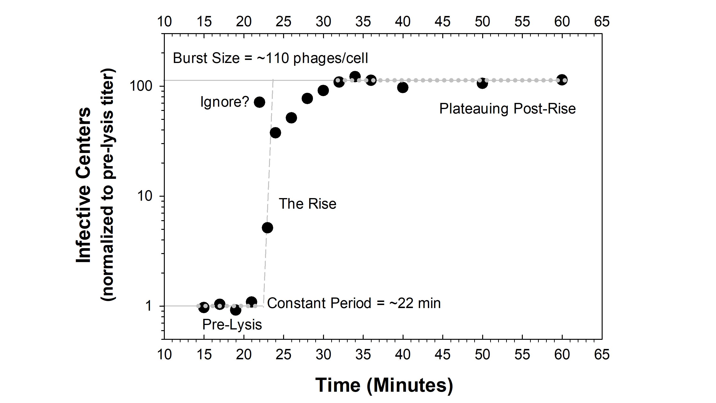
Here we present various considerations on both how to and how not to perform these very basic phage-characterization experiments. For specific, more-detailed protocols, see for example Hyman and Abedon [35] and Kropinski [7], plus [1,4,5,42] as well as the methods provided here in the following section (2.3) and in Section 4. See Figure 1 and Appendix A for a number of examples of OSG curves obtained from the Creative Commons literature along with extensive critiques of those experiments and their presentation. See Table 1 for definitions.
2. One-Step Growth Curve Determination
Perhaps not surprisingly, there are two key aspects that must be considered when performing OSG experiments: the “one-step” aspect and the “growth” aspect. In this section we consider these two fundamental aspects of OSG as well as outline a basic OSG protocol.
2.1. ”Growth” Is the Easy Part
The more straightforward part of OSG, and also what seems to be both generally understood and correctly presented in publications, is the “growth” aspect. This, for phages, is simply the product of a successful lytic infection [11], or more formally, it serves as a basic unit of phage population growth. Rates of phage population growth, as noted above, are dependent on a combination of phage adsorption rates, phage latent period lengths, and phage burst sizes as well as rates of virion decay. Specifically, it is effectively universally the case that published OSG experiments reveal the occurrence of rises in phage titers over time, at least when following phages associating with bacteria that are found within their host ranges. This rise in titer is the noted phage population growth.
2.2. ”One-Step” Is Trickier
The “one-step” part of OSG experiments is something that publications often seem to struggle with (e.g., see Appendix A) and which therefore is a primary emphasis of this Perspective. OSG thus specifically, and at a minimum, involves the passage of a population of phages through only a single round of bacterial infection and subsequent virion release. Usually this process, after setup of the experiment (Section 3.1), begins with adsorption of that phage population to a pure broth culture of bacteria (Section 3.2), though alternatively it is possible to initiate phage lytic cycles with induction of bacterial lysogens (Section 5.1). The process then progresses through a post-adsorption, pre-lysis determination of numbers of phage-infected bacteria, traditionally described as infective centers (Section 3.3). This is followed by what is known as the phage rise, which is the time during which lysis and therefore release of free phages from phage-infected bacteria is occurring, i.e., constituting a ‘rise’ in phage titers (Section 3.4). Importantly, these free phages are also described as infective centers. Lastly, there is a plateauing of phage titers that defines the post-lysis period of OSG (Section 3.5). In broad outline, this is adsorption, infection, lysis, and then stabilization of phage titers, thus completing one-step growth (Section 3.6). Note, however, that if phage adsorption is allowed to follow this single step of phage population growth, then instead it is multi-step growth that is being observed (Section 3.5.1).
2.3. A Basic One-Step Growth Protocol
The classic OSG method, as provided by Ellis and Delbrück [2], consisted of the following. From their p. 376:
[i] A suitable dilution of phage was mixed with a suspension of bacteria containing 2 × 10⁸ organisms per cc. and [ii] allowed to stand at the indicated temperature for 10 minutes to obtain more than 90 per cent adsorption of the phage. [iii] This mixture was then diluted 1:104 in broth, and incubated. [iv] It was again diluted 1:10 at the start of the first rise to further decrease the rate of adsorption of the phage set free in the first step.
As experimental output, [v] “Relative phage concentration” was reported.
That protocol is quite simple and is at least arguably sufficiently comprehensive. The goal of this perspective therefore is less toward providing a “cookie-cutter” OSG protocol, though see Section 4 as well as the references cited at the end of the Introduction for additional protocols. Instead, the goal is much more toward getting phage researchers to think about how to more effectively perform and then present their OSG experiments. As a first step toward these goals, what follows is some detail added to the Ellis and Delbrück [2] protocol, with equivalent Roman numerals provided for guidance.
Needed to begin with (Section 3.1) are a titered phage stock, a culture of experimental bacteria that the phage is able to infect, and a culture of indicator bacteria which is able to effectively plaque that phage, i.e., with high efficiencies of plating [1,4,43,44]. Neither the bacterial strains – experimental vs. indicator – nor their means of preparation have to be identical (bacterial strains can differ and so too can methods of bacterial strain preparation). As noted, what follows corresponds to the Ellis and Delbrück [2] protocol, and this is rather than explicitly following the arrangement of steps found in Section 3:
- Add phages to a broth culture of experimental bacteria, usually with a starting ratio of added phages to targeted bacteria of one-tenth (0.1) or less. Typically this broth culture will be in mid-log phase, though it is certainly possible to intentionally vary from that.
- Allow for phage adsorption, which ideally will occur over a relatively short span of time, such as a few minutes, and which, as noted by Ellis and Delbrück, ultimately should be fairly complete before proceeding further.
- Prior to the anticipated start of lysis and after sufficient adsorption has occurred, dilute cultures. It is necessary to dilute at this time to minimize the adsorption of released virions to still-present bacteria, thereby avoiding multi-step growth. It also is convenient to perform this dilution prior to the next step, step iv, so as to minimize subsequent diluting before plating. This is a step that seems most often to be missing in published OSG methods, typically leading to the appearance of multi-step rather than single-step growth (Section 3.5.1 and Appendix A).
- It can be both useful and convenient to further dilute cultures in anticipation of phage release, where such release constitutes the phage rise. This dilution step (or steps) especially needs to be precise since any diluting errors at this point will directly impact calculated burst sizes.
- Throughout this process, take samples for plating, starting particularly after step iii. This is the determining-numbers-of-infective-centers step.
How to calculate minimum latent periods is described in Section 3.4.5 and Section 3.6.2. How to calculate average burst sizes is presented in Section 3.5.4.
Note that details such as the timing of dilution steps will vary depending on the system being characterized as well as with personal preference. Our intention over the course of much of this piece is to ensure that the above steps successfully yield accurate and precise determinations of phage latent periods and burst sizes. Further protocol detail is provided in Section 4.
2.4. Summary of Dos and Don’ts
As a guide to much of the rest of this piece, we provide the following summary of one-step dos and don’ts, with relevant sections supplying detail indicated parenthetically:
- Do run simplified pilot experiments toward subsequent OSG design, including as based on culture turbidity measures alone (4.3).
- Do start with a reasonably fresh phage stock (3.1.2).
- Do titer using fresh (3.1.4), log-phase indicator bacterial strain (3.4.1), which also support a high efficiency of free phage plating (3.1.3).
- Don’t initiate experiments with phage multiplicities of greater than 0.1 (3.2.2).
- Do optimize phage adsorption toward increasing adsorption synchronization (3.2.3).
- Do titer for free phages post-adsorption and/or remove those phages from experimental cultures (3.3.2, 3.3.3, 3.5.4.1).
- Do generate sufficient numbers, e.g., 5, of pre-lysis titer time points (3.4.4, 4.13).
- Do dilute experimental cultures sufficiently to avoid multi-step growth (3.3.4, 3.5.1).
- Don’t dilute experimental cultures so far that too few bacteria are being sampled for lysis (3.3.4).
- Do design dilutions to minimize diluting complications during experiments (Section 4).
- Don’t worry too much about keeping intervals between time points consistent (3.4.3).
- Do increase the number of time points around when lysis (the rise) is expected to take place (3.4.4).
- Do use the point at which the rise has begun to define the end of the constant period (3.4.5), unless the jump in titer is too great (3.3.6), and consider using the trajectory of the rise also or instead to estimate this time point (3.4.5, 3.6.2).
- Don’t claim lysis-timing precision that exceeds the length of intervals between time points (3.4.2, 3.4.5).
- Do keep in mind that the duration of the rise in part is a function of how well initial phage adsorptions were synchronized (3.2.3).
- Do make sure that phage titers have plateaued post-rise (3.5.2).
- Do take multiple time points during the post-rise (3.5.4), such as over a half-hour period.
- Do follow up on unexpectedly or unusually large burst sizes (3.6.3).
- Do present data normalized to average starting phage titers so as to make burst sizes more easily appreciated visually (3.5.3).
- Don’t add chloroform to infective center-containing media at any point during experiments except within a separate containing prior to plating for unadsorbed phages (4.1.2), or if the goal is to define the eclipse (5.3), or instead to validate the post-rise (5.2).
3. One-Step Dos and Don’ts
In this section, we provide guidance toward improving the execution of OSG experiments. We do this in a narrative form rather than providing as a series of explicit OSG “dos” and “don’ts”, which are found instead in Section 2.4, immediately above. Major headings correspond to “Experimental Setup” (Section 3.1), “Phage adsorption” (Section 3.2), “Post-adsorption, prior to lysis” (Section 3.3), “During lysis (the rise)” (Section 3.4), and “After lysis” (Section 3.5). We then provide a sub-section titled, “What data are important” (Section 3.6). See Figure 2 for a summary of some of the concepts considered in this section. In Box 1, we also present a published, though here anonymous, example of what sorts of things often can be improved upon during experimental one-step growth.
3.1. Experimental Setup
Discussed in this section are suggestions to consider implementing prior to the start of experiments.
3.1.1. Use Log Phase Experimental Bacteria
Two distinguishable bacterial cultures are used in one-step growth experiments, the experimental culture and the indicator bacteria. The latter are used to support phage plaquing. Considering just the experimental bacteria, the goal should be, with OSG, for those bacteria to display the physiology that one is interested in for phage characterization. Typically this would be mid-log phase. Generally, unless that is one’s specific interest, it should not be lag phase experimental bacteria that are used, meaning don’t just add overnight cultures to fresh media and then, after some only short span of time, start experiments (as was possibly done in the OSG assays discussed in Box 1).
Kropinski [7] suggests simply growing bacteria to mid-log phase and then, presumably, immediately starting the experiment, using that bacterial culture directly while continuing to incubate it at the same temperature it was grown at, including starting with a pre-warmed experimental flask. It is certainly permissible to explore different bacterial physiologies over the course of a series of OSG experiments, if that is one’s intention. Just make sure that bacterial physiologies are consistent both during individual experiments and from day to day. It is also permissible to use different types of broth to grow bacteria to log phase, e.g., Hadas et al. [45], such as for comparison between different growth conditions or instead to better mimic conditions found in situ.
Box 1. Example of a Problematic One-Step Growth Protocol.
In a recent, 2025, article – published in a reasonably noteworthy journal (impact factor ≈ 3) but which we otherwise are not citing for reasons of anonymity – two OSG curves are presented in which we have identified a number of errors. It is noteworthy, however, that these authors did separate unadsorbed virions from phage-infected bacteria (Section 3.3.2 and 3.5.4.1), as actually is fairly often done, but the experiment otherwise seems to possess the following issues:
- The experiment was initiated with stationary phase bacteria (“an overnight host”; Section 3.1.1).
- The experimental bacterial culture, at least as indicated, was not diluted during the experiment (Section 3.3.4), except that bacteria were suspended in fresh broth following phage adsorption and removal of free phages via centrifugation.
- Prior to the start of lysis, the number of infective centers rises somewhat, perhaps as we speculate due to phage infections of initially metabolizing stationary phase bacteria being detrimentally affected by the plating process.
- Five-minute time points were used throughout the experiment, including during the rise, resulting in only a single time point definitely capturing the lysis event (Section 3.4.2 and Section 3.4.4).
- Latent period is defined as the last pre-lysis time point, though in one case whether it is prior to or following that time point is ambiguous and in both cases, with five-minute time points it is difficult to say whether the start of lysis actually occurred at the indicated time point or instead occurred a few minutes later (Section 3.4.5).
- The burst size, at least diagrammatically, is defined as the first time point at which titers seem to start to stabilize, possibly post-lysis, rather than involving multiple post-lysis time points (Sections 3.4.4 and 3.5.5?).
- It is difficult for the reader to determine which time points were used to define the post-lysis phage titer in burst-size calculations.
- Phage titers are graphed as seemingly arbitrary values in absolute terms, i.e., starting around 103 PFU/ml. What do these titer values mean?
- Ideally these values would have been normalized to the pre-lysis phage titers in the presented figure (Section 3.5.3).
- Post-rise, the titer does not appear to stabilize but instead continues to increase (Section 3.4.4, Section 3.5.1, and Section 3.5.2).
This latter titer increase is only slight (point 10), though has been visually minimized in the figure by having the curve graphed using a log-transformed y axis. This, log-transformation of the y axis, indeed is something that we recommend (Section 3.4.5, Section 3.6.1, and Section 3.6.2), but which also for some aspects of figures can be obscuring, such as in this case of the ongoing increase in titers following lysis. Nonetheless, such an increase is inconsistent with the lack of pre-lysis diluting, which ought to give rise to more robust multi-step growth. That is, given the speculated lack of diluting, we would expect a greater post-rise ongoing increase in phage titers than we actually observe.
We have two possible explanations for that contradiction. First, perhaps the authors did in fact dilute, which is supported by their having taken more time points throughout the experiment than they seemingly had volume – as indicated in the methods – to take from. The one-step protocol they cite, however, also does not describe diluting, and also shows a somewhat consistently increasing titer between 20 and 130 or so minutes. The protocol this cited article cites in turn cuts off the experiment prior to the time of any ongoing increase in phage titer might have occurred. The second possibility is that multi-step growth was occurring, but that it was not robust due to the OSG experiment taking place using high, overnight-culture concentrations of bacteria. The bacteria thus were presumably able to use up the nutrients available in the added broth fairly quickly, particularly after entering into a lag phase, resulting in some but not much post-rise titer increase.
Overall, our opinion from this analysis is that this OSG curve, as well as the one these authors directly cite, is sufficiently flawed to be insufficiently useful toward either latent period or burst size determination. It is because of the existence of such OSG efforts and others (Appendix A) that we have undertaken the effort provided here.
3.1.2. Start with a Reasonably Fresh Phage Stock
To the extent that phage infection characteristics do not change during storage, then this second consideration may be ignored. Nevertheless, for the sake of consistency from experiment to experiment, or from laboratory to laboratory, it can be useful to define a specific phage stock age as standard, with freshly generated, e.g., not multiple years old, a reasonable standard. Particularly important is to avoid using phage stocks whose killing titers [46] greatly exceed numbers of PFUs. That is, it is helpful for numbers of adsorbing phages to be similar to numbers of viable phages, so as to avoid varying multiplicities of adsorption between phage stocks (this more generally is an issue of low phage efficiency of plating, as considered in the following section, 3.1.3). Note also that virions can potentially aggregate over time during storage, but which can disaggregate over the course of incubation at, e.g., 37°C [47].
It is important regardless to make sure that a phage stock’s titer has been determined reasonably recently prior to OSG, since starting titers and multiplicities of infection (MOIs) are important for the mechanics of OSG determinations. Ideally, that is, it will be possible to anticipate how many plaques will be found on plates, particularly prior to OSG lysis. For more on MOIs, see [48,49,50]. Considered in the following section (3.1.3) is why avoiding unexpectedly high MOIs can matter when performing OSG experiments.
3.1.3. Taking into Account Phage Efficiency of Plating
Related to the above idea that phage plating titers (PFUs) and phage killing titers ideally should be similar – the latter being numbers of phages calculated in terms of their abilities to kill bacteria rather than their abilities to form plaques [46] – is an issue of phage efficiency of plating (EOP) [1,4,43,44]. Phages whose killing titers exceed their plating titers will have EOPs of less than one, at least in terms of absolute efficiency of plating [1,4]; that is, more phages able to adsorb and kill than are able to form plaques. Low EOPs could be present perhaps especially if stationary phase rather than log phase indicator bacteria are used for titering of phage stocks (Section 3.4.1).
If EOP is low, then the result will be starting phage multiplicities that, in terms of phage adsorptions, are greater than anticipated based on PFU counts alone. Though in practice this issue is perhaps almost never considered when performing OSG experiments, it still could be relevant. It therefore should not be completely ignored, and this is so especially if the phage being characterized is able to display lysis inhibition.
Lysis inhibition is a multiple phage adsorption-induced extension of the phage latent period, resulting also in an increase in the phage burst size [51]. In particular, a phage displaying a low EOP on the titering host, and which also displays lysis inhibition, could register unexpectedly long single-step latent periods as well as larger burst sizes, due to excessive phage adsorption. Indeed, an important reason that OSG experiments are initiated with MOIs of somewhat less than one is to avoid induction of lysis inhibition. We discuss in Section 3.4.1 another way that this issue of low EOPs can be relevant during OSG experiments.
3.1.4. Start with Fresh Indicator Bacteria
At a minimum, indicator bacteria should be reasonably consistent in terms of ability to support phage plaquing, going from experiment to experiment as well as over the course of individual experiments, the latter point considering especially EOPs for free phages vs. phage-infected bacteria. Thus, as a general rule, indicator bacteria, i.e., plating culture, should be made up fresh for individual OSG experiments. The properties of indicator bacteria are considered further in Section 3.4.1.
3.2. Phage Adsorption: A Time for Synchronization
The phage adsorption step during OSG involves adding phage virions to experimental, broth bacterial cultures and then, waiting. Ideally, this wait will be over after a relatively short interval (see “Synchronization…”, Section 3.2.3). For instance, Kropinski [7], p. 41, notes that OSG experiments are “based upon the assumption that 90–95% of the phages adsorb to the host cells within 5 min” Generally, the adsorption interval is terminated – at a minimum – by a substantial dilution of the experimental culture. Consequently, this necessary culture dilution, particularly step iii in Section 2.3, should not come too soon after phage addition to bacteria (minutes later rather than seconds later). As noted above (Section 2.3), this OSG-essential dilution step often appears to be missing from published OSG experiments. As a general rule, if there is no dilution of experimental bacterial cultures, then there is no one-step growth. See Section 3.5.1 for more on multi-step phage growth.
3.2.1. Use a Sufficient Concentration of Experimental Bacteria
It is bacterial concentrations that determine the rate at which individual phages adsorb, which is what is of concern at the start of OSG. This actually is the opposite of the concern with phage therapy, where instead it is the rate at which individual bacteria are adsorbed by that is relevant rather than explicitly how fast individual phages are adsorbing [52]. From Adams [1], p. 14, “1. Phage and bacteria are mixed at [bacterial] concentrations that permit rapid adsorption.” That statement, however, is complicated by the fact that having too concentrated a bacterial culture can result in undesired changes in bacterial physiology. Thus, more properly stated, one should be using experimental bacterial cultures that are sufficiently concentrated to allow for rapid phage adsorption, but not necessarily so concentrated that this impacts bacterial physiologies in undesired ways.
As indicated by Ellis and Delbrück [2], initial bacterial concentrations in the range of 108 per ml should be targeted, while Adams [1] instead suggests 5 × 10⁷ CFUs/ml. Keep in mind, however, that numbers of individual bacteria and numbers of colony-forming units (CFUs) are not necessarily identical. Note also that it should be possible to concentrate bacteria, if need be, prior to the phage adsorption step, such as concentration via centrifugation. This too, though, should be done in such a way that does not inappropriately impact bacterial physiological states. That is, the reason one does OSG experiments is to assess phage infection during growth on bacteria of a reasonably well defined physiology, so some thought and effort should go into retaining that physiology. In addition, handling of experimental bacteria certainly should be consistent from experiment to experiment.
3.2.2. Use an Appropriate MOI
As originally conceived, as well as subsequently developed, OSG experiments were intended to characterize not just a single round of phage infection but also to have that single round be dominated by infected bacteria that have been adsorbed by only a single phage, though Ellis and Delbrück [2] did explore as well multiple virion adsorption. Adsorption of every bacterium by only a single phage, under most circumstances, is however not possible to achieve absolutely across a bacterial population, and this is due to Poissonal distributions of virion adsorptions over targeted bacteria [5,49,52,53,54,55,56]. Nevertheless, singly infected bacteria can substantially predominate in cultures if starting MOIs are sufficiently low. Thus, an MOI of 1 will result in an anticipated 42% of phage-infected bacteria present having been adsorbed by more than one virion (of 63% of bacteria which in total are phage adsorbed, i.e., 1 - e-1, multiplied by 100 to make the value a percentage). Dropping the MOI to 0.1, however, reduces that percentage to only 5%. Specifically, in Microsoft Excel, use the formula, “=100*(1-(POISSON.DIST(1,n,FALSE)/(1-POISSON.DIST(0,n,FALSE))))”, where n is equal to the realized multiplicity of infection, i.e., an MOIactual such as 0.1.
Note that if attempting to perform OSG experiments using multiplicities of greater than one, then one has to be certain that CFUs consist of individual cells. The goal in other words should be to define phage multiplicities of infection explicitly as phages per cell rather than phages per CFU. If that is not the case, that is, if CFUs consist of more than one bacterium linked together (a cellular arrangement or bacterial microcolony), then one risks having individual infective centers consisting of more than one phage-infected bacterium. That in turn will have the effect of artificially increasing calculated burst sizes as well as result in multi-step growth—more phages produced per phage-infected CFU as MOIs are increased, but not necessarily also more phages produced per phage-infected bacterium, and with this phage production taking place over multiple phage latent periods. For possible evidence of this effect, see in particular the results of Gadagkar and Gopinathan [57], as discussed by Abedon and Thomas-Abedon [32]. An example of use of an MOI of greater than 1 can be seen in Figure 0045249 (Appendix A).
It nonetheless certainly is permissible to explicitly study the infection characteristics of multiply phage-infected bacteria. Regardless of what MOI is used, though, just make sure when adding phages that bacterial cultures do not become excessively diluted with phage buffer, as that would have the effect of possibly modifying experimental conditions to the detriment of accurate latent period and burst size determination.
3.2.3. Synchronization of Adsorption
OSG provides a description of population averages of phage characteristics rather than single-cell precision. It is possible alternatively to study single-cell lysis timing [58] or single-cell productivity (single burst experiment) [1,2,3,4,59], but these are more complicated to do. Nonetheless, OSG precision can be increased. One way to accomplish this, particularly for latent period determinations, is by taking sufficient numbers of time points, particularly at crucial times (Section 3.4.2 and Section 3.4.5). Synchronization of phage adsorption, however, is also important toward increasing that precision. From Adams [1], p. 441, “One-step growth of phage: A single cycle of infection and lysis, nearly synchronous in all the infected bacteria of the culture…” Specifically, the closer one can get to physiologically starting all phage infections at the same time, then the shorter the duration of the rise and the closer the rise is to describing the distribution of lysis timing across infections, vs. also the distribution of adsorptions.
Failure to employ one or more strategies toward synchronizing adsorption will result in artificially long rise periods due to more drawn-out adsorption. This is less of an issue if latent period is defined as the start of the rise rather than, e.g., its middle, and if the duration of the rise is not otherwise considered to be relevant to assay success. Excessively slow virion adsorption relative to the start of bacterial metabolism could, however, impact determinations of minimum latent periods, i.e., by delaying the beginnings of virion release. Thus, at a minimum, it is best to start with sufficient numbers of bacteria (Section 3.1.2), and then to halt adsorption relatively soon, particularly a few minutes after it has begun. Adams [1] used, for example, 5 minutes for pre-dilution phage adsorption, though noted that this may need to be longer for slowly adsorbing phages (see too Kropinski [7]). Adams also cautioned (p. 477) that, “The adsorption time is limited by the necessity of completing the dilutions before the end of the latent period.” For OSG curves suggesting a lack of adsorption synchronization, see for example Figures 0045242 and 0045243 (Appendix A).
3.2.4. Routes to Adsorption Synchronization
Synchronization of phage adsorption explicitly is in terms of phage-infection metabolism. That is, the goal is for as large a fraction of phages as possible to adsorb at something close to t = 0 for the OSG experiment. There are multiple approaches, not necessarily all mutually exclusive, to achieving such adsorption synchronization. One is to start, as noted (Section 2.2), not with virions at all but instead with bacterial lysogens that can be simultaneously induced (Section 5.1). That approach, though, only works with temperate phages.
A second synchronization strategy is to dispense with infection metabolism altogether, by adsorbing to temporarily metabolically inhibited bacteria [46]. This includes as can be accomplished by washing bacteria in media lacking in appropriate energy sources. A compromise is to simply slow bacterial metabolism by performing the adsorption step at a lower temperature, such as room temperature. The latter is an elaboration on Carlson’s [46] suggestion that the entire experiment might be performed at a lower temperature (see too Kropinski [7]), though if carried out over the entire OSG experiment that obviously would modify resulting phage growth parameter values, resulting, for example, in a lengthening of measured latent periods [2]. Note, though, that Carlson [5] cautions against such delays in plating as (p. 434) “chilling cells or using growth inhibitors… usually gives less reproducible results.” Kropinski [7] similarly states, “We do not recommend chilling the phage-host mixture.”
A third and probably most-standard approach is to use both sufficient concentrations of bacteria and sufficiently permissive adsorption conditions that the adsorption process itself is rapid (Section 3.1.2).
A fourth approach, also fairly standard and not mutually exclusive, is to stop adsorption after a relatively brief period of time. This can be done by either diluting bacteria (though with the issue that free phages will remain in the media), selectively killing free phages using virucides [60], or using specific anti-virion serum [3]. Alternatively, it is possible to physically separate free phages from bacteria as can be accomplished via centrifugation. Note if doing the latter that it is the supernatant that is discarded and the pellet that is kept; for a possible example where instead the pellet may have been discarded, at least in the course of titering, see Figure 0045249, Appendix A. Adams [1], p. 14, indicates this adsorption stopping process as, “2. After a suitable adsorption period the mixture is diluted into antiphage antibody to stop adsorption and inactivate unadsorbed phage.” Stent [4] too suggests the use of antiphage serum, though more recent protocols have not.
3.3. Post-Adsorption, Prior to Lysis: The Phage Infection
Steps to be taken prior to the start of lysis, especially once adsorption has been stopped, include providing any additional necessary dilutions of the phage-infected bacteria and to plate for PFUs. Plating for PFUs requires that unadsorbed free phages be excluded from those counts. As noted above, it is the necessary dilution step that seems to be most-often missing from problematic OSG experiments.
3.3.1. Infective Centers
As noted, traditionally PFUs in the context of OSG were referred to not as PFUs but instead as infective centers [1,2,4]. This was done so as to not distinguish explicitly between plaques initiated by free phages vs. plaques initiated instead by phage-infected bacteria. From Adams [1], p. 440, “Infective center: A plaque-forming particle that may be either a productively infected bacterium or a free phage particle. When one or the other is meant, the term infective center should not be used.” We will use “Infective center” here as appropriate, but it can be interpreted as equivalent to PFU. Its use is relevant particularly in this section, however, since what is being enumerated, post-adsorption and prior to lysis, are plaque-forming units that consist (ideally) of just phage-infected bacteria rather than also unadsorbed virions.
3.3.2. Accounting for Free, Unadsorbed Phages
From Adams [1], p. 15, “If unadsorbed phage were not inactivated the early plaque counts would include unadsorbed phage as well as infected bacteria and the estimate of the burst size would be too small.” The suggested use of anti-phage antibodies, or instead using virucides, or use of centrifugation (Section 3.2.3), are all for the sake of eliminating free phages early during OSG experiments. More generally, however, these are approaches to achieving a broader aim, which is one of properly accounting for unadsorbed free phages, something which can also be achieved by assessing for free phages after the adsorption period.
Eliminating free phages such as by using anti-phage serum or virucides should be done prior to the initial plating for infective centers. If free-phage inactivation is used, though, then it is important to dilute away the inactivating agent subsequent to both plating for infective centers and the phage rise (for the latter, see Section 3.4). It also is helpful to employ a free-phage assessment step (Section 3.3.3) even when using the aforementioned virucides, etc. Assessing for remaining free phages should be done after cultures have been diluted rather than prior to diluting, as diluting serves as a means of lowering the concentrations of antibodies or virucides, if present, as well as serving as an alternative means of substantially reducing ongoing phage adsorption. Such plating for free phages, though, does not necessarily need to be done explicitly prior to plating for infective centers, as further phage adsorption during experiments, following diluting of the experimental culture, is unlikely. On the other hand, it is important to complete this assessment for free phages prior to the start of the rise. Given both culture dilution and plating for unadsorbed virions, explicit free phage inactivation to stop phage adsorption in most cases is not essential.
The goal in any case is to account for free, unadsorbed phages so as to make sure that their numbers are not included among the infective centers that are being enumerated prior to the start of lysis. Burst sizes, in other words, are determined by dividing numbers of free phages that are present post-lysis (specifically, post-rise) by numbers of phage-infected bacteria that are present prior to that lysis (Section 3.5.4). Especially the latter, pre-lysis phage numbers, can be exaggerated by the presence of free phages, so those must in some manner be accounted for, i.e., subtracted off from total, pre-lysis number of PFUs. Numbers of post-rise free phages can be impacted as well by these numbers of initial, unadsorbed phages. That, however, is less of a problem [61] unless phage adsorption has been particularly poor or burst sizes excessively small, i.e., since otherwise the impact of inclusion of those pre-lysis unadsorbed phages in counts of post-lysis phage numbers will tend to be trivial.
3.3.3. Assessing Unadsorbed Phages
Perhaps the easiest way to assess for unadsorbed virions is to use centrifugation to remove bacteria, including phage-infected bacteria, and then to titer the resulting supernatant [1]. This should be done well prior to the start of lysis, however, so as to minimize the likelihood of inadvertently releasing free phages from infected bacteria. Alternatively, one can use chloroform to kill phage-infected bacteria while sparing free virions or instead can sonically disrupt bacteria toward the same end [1]. This is at least to the extent that those treatments don’t also disrupt virions [7,62] and note also that such cell disruptions not necessarily occurring with 100% efficiency [61]. These latter approaches, however, are limited to being used prior to the end of the eclipse, since lysis of phage-infected bacteria after that point by definition will release intracellular virions into the extracellular environment (Section 5.3).
One can inactivate virions, such as by adding virucide, and then plate for remaining infective centers, looking for differences in titers with and without such treatment. That approach, however, will tend to provide a less definite indication of how many phages had remained unadsorbed. In any case, ideally at least two or three plates, from different dilution series if dilution series are used, should be run to determine the quantity of unadsorbed virions, so as to minimize operator error [63]. What certainly should not be done is to just assume, without supporting evidence, that the number of phages added will be equal to the number of bacteria infected.
3.3.4. Dilute Enough, but Not Too Much
From Adams [1], p. 14, “3. After sufficient time for antibody action”, or otherwise removal of virions by other means or accounting for free phages, “the mixture is further diluted in growth medium so that each sample will contain about 100 infected bacteria.” This dilution specifically is done prior to the start of lysis, but it is important also not to dilute too much. The latter is so as to avoid excessive variability due to sampling error, which is expected to be 10% with a minimum count of 100, such as of phage-infected bacteria. This is equal to the square root of the mean [1,64], something that is greater with lower numbers, e.g., 14% for a count of 50 or 20% for a count of 25. Also important, burst sizes will vary between phage-infected bacteria [59], so the fewer bacteria supplying bursts, such as less than 100 phage-infected bacteria, then the more likely that burst size determinations could be skewed by rare, especially larger bursts.
As suggested by Ellis and Delbrück [2], this dilution should be on the order of 10,000-fold. So too Stent [4] suggests 40-fold dilution into media containing antiphage serum and then another 250-fold into serum-less media (40 × 250 = 10,000); see similarly Carlson [5,46] but without the exposure to serum, as nor do Ellis and Delbrück suggest use of anti-phage serum. If one started with 108 bacteria/ml, adsorbed 107 phages/ml to these bacteria, and diluted the mixture the indicated 104-fold, then you would expect to have a total 103 phage-infected bacteria/ml. That can then be conveniently titered by plating 100 μl volumes (Section 4). If instead an MOI of 0.01 is employed, then that number would be 102 phage-infected bacteria/ml, requiring plating using 1 ml volumes. If the phage being used is slow to adsorb, then the number of phage-infected bacteria could be even lower, also requiring either less diluting prior to plating or instead plating greater volumes.
Hyman and Abedon [6] by contrast suggested a 2,500-fold initial dilution rather than 10,000-fold dilution. This has the effect of increasing initial platings to average an anticipated 400 PFUs/plate, which has a minimum expected error of 5% rather than the 10% for an average of 100 PFUs/plate. Of course, it also has the effect of increasing plaque-counting efforts. While Ellis and Delbrück [2] suggested instead the noted 10,000-fold dilution, they also started with 2 × 10⁸ bacteria/ml, a two-fold greater bacterial concentration than that suggested by Hyman and Abedon. With an MOI of 0.1 and near-complete adsorption, Ellis and Delbrück’s approach would yield roughly 200 infected bacteria prior to lysis per 100 μl plated. Thus, there are no hard-and-fast rules as to what starting bacterial concentrations, phage MOIs, or fold-dilutions to use, just so long as phage adsorption is adequate and that with the first dilution step one ends up with neither too few nor too many phage-infected bacteria (Section 3.3.5). It in other words is important to think through diluting issues in designing OSG experiments, as addressed in more detail here in Section 4. For examples of OSG curves in which diluting may not have taken place following phage addition, see Figures 0045243, 0045248, 0045249, 0043940, 0044206, 0042333, 0044790, and 0045021 as well as Figure 0039663 (Appendix A).
3.3.5. Reducing Post-Lysis Adsorption
Also from Adams [1], p. 15, “The dilution of the adsorption mixture at the end of the adsorption period is an essential feature of the experiment because it prevents further adsorption.” Thus, if the amount of dilution is insufficient, then phages that are released upon lysis will be too likely to adsorb either infected or uninfected bacteria, due to some combination of too high resulting concentration of phages and too high remaining concentrations of bacteria. (Recall that uninfected bacteria should exceed infected bacteria in number by at least ten-fold when striving for multiplicities of 0.1 and also that uninfected bacteria can replicate in the course of OSG.) Though such additional adsorption would occur only post-lysis, the concern is included in this section because the actual dilution needs to be made pre-lysis.
Adsorption of already phage-infected bacteria can result in induction of lysis inhibition for those phages that are capable of displaying that phenotype (Section 3.1.3). Multi-step rather than only single-step growth alternatively is the consequence of adsorption by released phages, post-lysis, of phage-uninfected bacteria (Section 3.5.1). Either of these can result in overestimations of phage burst sizes and sometimes these overestimations can be dramatic. Be concerned especially if the rise seems to take place in multiple steps or instead if burst sizes, at least for most phages, are much greater than roughly 500. Certainly burst sizes of 1,000 or more should almost always be viewed as red flags, though with some exceptions (Figure 1 and Section 3.6.3). Also, the larger the burst size, then the more likely that released phages will adsorb still-intact bacteria. See Section 3.5.1 and Section 3.5.2 for additional discussion of these issues.
A further advantage of this post-adsorption, pre-lysis dilution step is that it eliminates a need to aerate cultures, since resultant bacterial densities are so low [5,46]. That, of course, assumes that the media is already aerated, but such aeration can be assured via vortexing in the course of this diluting. See Box 1 where we speculate that a failure to sufficiently dilute could have led, e.g., to poor oxygenation of bacteria later in experiments.
3.3.6. Bacteria Can Lyse During Enumeration
Something that can occur upon plating of seemingly still pre-lysis cultures is the lysis of phage-infected bacteria, particularly as OSG experiments get closer to the start of the rise. As a consequence, for example, long delays between sampling and plating can give rise to latent period underestimations, with the timing of sample acquisition differing somewhat from the timing at sample plating. Such events can result in unusually high plaque counts, i.e., unexpectedly large jumps in these counts that also don’t follow the otherwise smooth increase in titers normally seen during the rise. Adams [1], p. 481, as a consequence wrote that “any point along the rise portion of the single step curve may lie well above the curve. Since there is no compensating error which may lead to correspondingly low counts, these high points must be disregarded in drawing the curve. … If this is included in the average value used to calculate the burst size, it may lead to significant error.”
3.4. During Lysis: The Phage Rise
During lysis, plating for infective centers should take place as a continuation of especially late pre-lysis enumeration, since generally the reason that OSG enumeration is being undertaken is that we don’t precisely know when the start of lysis is going to occur. This plating for plaques should continue through to the end of lysis, and then some, with the span from start to finish of this lysis known as the rise. It certainly is possible to learn from previous OSG experiments, i.e., prior biological repeats, just when lysis is expected to occur, especially its beginning, and then adjust the timing of ones plating accordingly (e.g., see Section 4.1).
3.4.1. Use Log-Phase Indicator Bacteria
It is not uncommon to use stationary phase bacteria, such as overnight cultures, as indicator for titering [65]. A concern here is that efficiency of plating might vary as a function of the physiology of indicator bacteria, particularly often declining with the use of stationary-phase rather than log-phase bacteria, though not always [66,67]. In addition, however, EOPs can vary with the state of the potential plaque-forming units [66]. Specifically, a plaque should be more likely to form starting with, e.g., 100 phages released from a just-plated phage-infected bacterium than from an isolated virion. As summarized by Adams [1], p. 494: “The relative efficiency of plating of infected bacteria is usually higher than that of free phage, so both should be determined.” Thus, using, e.g., stationary phase indicator bacteria could have the effect of reducing measured burst sizes, which explicitly during OSG are ratios of free phages (potentially displaying lower EOPs) to phage-infected bacteria (potentially displaying higher EOPs) (Section 3.5.4).
The previous point can be generalized to concerns over efficiencies of plating that are reduced by any mechanism (Section 3.1.3). As the primary concern is that of differences between the plating efficiencies of free phages vs. phage-infected bacteria, this issue can be readily checked experimentally and then accommodated in calculations as needed. For example, compare the titers of pre-adsorbed phages [67] to directly plated free phages. Ideally those titers will be the same. But even if they are not the same, their ratios can be used to adjust burst size calculations [66]. Nonetheless, it is probably good practice simply to avoid using stationary phase bacteria as indicator when generating OSG curves, unless efforts are made to assure that it doesn’t impact free phage vs. phage-infected bacteria efficiencies of plating.
3.4.2. Too Many Time Points Is Preferable to Too Few
Adams [1], p. 14, states, “4. The suspension of infected bacteria is sampled at intervals until lysis is completed and each sample is assayed by the plaque count method.” Note, though, that no mention is made in that statement of either when or how often to sample. Though subsequently addressed by Adams (time points in the example presented by Adams were taken every 1 to 2 min for much of the assay), over the years many researchers, in our opinion, have become overly obsessed with ‘when’ and insufficiently concerned with ‘how often’. Thus, and though seemingly obvious, our experience has been that this still has to be stated explicitly: The precision of the lysis timing event should be directly proportional to the length of intervals between time points. In this section we thus consider ‘how often’, whereas in the next two sections (3.4.3 and 3.4.4) we address ‘when’.
In terms of how often, if OSG experiments are sampled every five minutes, then it can be difficult to describe measured latent periods – particularly the length of what is known as the constant period, i.e., which ends at the start of the rise – in any less than five-minute units (e.g., 10, 15, or 20 min). Certainly, it is not permissible to conclude that measured latent periods were, e.g., 18 min after having taken five-min time points. Thus, Adams [1], p. 475, states that if “plaque counts… are constant through 21 min[,] but increase suddenly by 23 min[,] so the end of the latent period comes between 21 and 23 min.” The conclusion, in other words, should not be, e.g., 22 min (though see Figure 2 where for convenience we conclude just that). See though Section 3.4.5 for a possible contradiction to this latter statement, but one requiring more rather than fewer time points. If high precision is desired, and we certainly hope that it would be, at least following pilot experiments, then consider taking additional time points especially while lysis is thought to be occurring. Indeed, feel free to take as many time points as you can in the time-vicinity of especially of the initial lysis event (Section 3.4.4).
Adams in his example takes time points every minute from 19 to 26 minutes, as encompasses the start of lysis, as occurred indeed at 22 min. In addition are four time points taken prior to lysis. Doermann (1952) took at least 25 time points over 25 min (10 to 35 min) in the OSG experiment he presents. This includes over 10 time points prior to lysis and at least 8 time points during the rise, seemingly taken at random intervals. Of course, there are only so many time points that can be taken especially at the start of lysis, since the interval over which this occurs is short. Nevertheless, there is nothing stopping one from taking as many time points during this brief, rise-initiating interval as one possibly can.
3.4.3. It’s Not Essential to Keep Intervals Between Time Points Constant
Time points need to be taken for OSG experiments during three distinct, post-adsorption periods: prior to, during, and following phage-induced bacterial lysis (Section 3.3, 3.4, and 3.5, respectively). There is no inherent reason, however, that the intervals between time points should be identical during these distinct periods. We note that this statement seems to contradict Kropinski’s [7], p. 41, indication of an importance to “following a rigid time frame.” Kropinski in his example OSG experiment, however, uses 2-min time points. Therefore, to clarify: Not keeping intervals between time points “Rigid”, as suggested in this section, is a means of reducing the overall number of time points taken. Unfortunately, exploration of phage publications (e.g., see Appendix A) suggest that many researchers have used this notion of a desire for rigidity toward reducing the number of time points taken overall, e.g., by using 5-min rather than the 2-min rigid time point intervals used by Kropinski. Indeed, Kropinski goes on to note (p. 46): “After running your experimental OSG experiment the first time you will be able to judge how often you should sample and from which flask. To make sampling easier, an overlapping timing of sampling from each flask is recommended.” Thus, we both recommend not explicitly following the advice for rigidity provided by Kropinski while at the same time commending the effort he put into assuring OSG precision.
Notwithstanding that latter point, and as emphasized in the previous section (3.4.2), reducing intervals between time points should be encouraged. This is particularly when lysis is thought to be occurring, i.e., during the phage rise and especially at the start of the rise (the latter defining the end of the constant/minimum latent period). That is, quite the opposite of following a rigid plating schedule. Nonetheless, clearly using multiple, different time point intervals over the course of a single experiment can be complicating. One solution is to record time points as they are taken, as seems to be the case in the classic, Doermann (1952) OSG experiments and see also the OSG example found in Adams [1]. This is rather than limiting time points to explicit intervals, e.g., every five minutes (as an aside: OSG curves using five-min time intervals should never be acceptable for publication except for viruses that display very long latent periods, e.g., of roughly one hour or more).
At the same time, this somewhat more unstructured approach to taking time points can lend itself to both not delaying platings and not plating individual time points multiple times per experiment, two things we recommend (Section 4). To present multiple experiments having non-overlapping time points in the same graph, if that is desired, then one can simply show all of the time points taken – also something that we encourage – rather than indicating individual time points as averages. Taking that approach, however, requires normalizing titer outputs, which is something that we suggest regardless (Section 3.5.3).
3.4.4. Take Sufficient Numbers of Time Points at Each Stage
During all three post-adsorption OSG stages, phase, or periods, sufficient numbers of time points should be taken. For example, up to five, if not even more, for each of these periods, for a total 15 time points, and ideally even more. There are, however, different reasons for taking numerous time points during each period.
Following adsorption and prior to lysis (Section 3.3), the goal is to be highly sure of what is the initial number of phage-infected bacteria. This will be your denominator in burst size calculations (Section 3.5.4), as well as the number to normalize to when comparing experiments (Section 3.5.3). See Section 3.5.3 as well for discussion of how you may go about generating those pre-lysis determinations of representative numbers of infective center.
During lysis (this section), the precision of your determination of the start of lysis, as the end of the constant period, will be highly dependent on the extent to which you succeed in catching the start of that lysis. Alternatively, catching the start of lysis can depend on how effectively you are able to graph the rise overall (see Section 3.4.5 for the latter). Thus, taking only five time points may not be enough over the course of the rise, and certainly will not be enough if the goal is to precisely characterize the extent of the rise, unless that interval is very short.
Following lysis (Section 3.5), it is important again to take a reasonable number of times points. This should be done for a number of reasons: (1) To assure yourself that the rise really has ended, (2) to better determine post-lysis phage titers, and (3) to make sure that post-lysis phage titers have stabilized rather than continue to rise (Section 3.5.2). All three, but especially (1) and (2), need to be done for the sake of burst size determinations (Section 3.5.4), while (3) is needed to make sure that experiments don’t involve more than one step (Section 3.5.1), or indeed aren’t displaying lysis inhibition (Section 3.1.3). It will tend to be easier to accomplish these goals if more time points are taken post-rise rather than fewer. Examples of OSG curves in which too few time points were taken during one or more periods of OSG include Figures 0045242, 0045243, 0045246, 0042856, 0045247, 0045248, 0045249, 0043940, 0043940, 0034153, 0039663, 0045245, 0044206, 0045250, 0039663, 0042333, 0044790, and 0044790, 0045021 (Appendix A).
3.4.5. Defining the Constant Period
Adams [1], p. 14, states, “The latent period is defined as the minimum time between the adsorption of phage to [the] host cell and the lysis of the host cell with release of phage progeny”. This places the end of the phage latent period, or what here we are describing as the minimum phage latent period, at the start of the rise, where minimum latent period is also called a constant period. Since the start of the rise is a specific time, the more time points that are taken during an OSG experiment, then the more precisely the minimum latent period can be determined. The alternative would be capturing the rise in its entirety with a single time point, such as is the case in the example described in Box 1 (and see also Appendix A, Figures 0045243, 0045249, 0034153, 0039663, and 0039663).
That is, consider this progression: the titer is the same as pre-lysis (first time point), then the titer is above the pre-lysis titer (second time point), and then the titer is the same as post-lysis titer (third time point). With only a single time point being intermediate between the pre-lysis and post-lysis phage titers, then at best one can declare that the rise began and ended sometime between those two extremes (pre-lysis and post-rise). This is instead of the rise corresponding in some way to that single, intermediate, during-rise time point. In other words, if lysis hasn’t occurred by 20 min, has started by 25 min, and has more or less been completed by 30 min, then there is no justification for declaring that the rise spanned those ten minutes nor, and more to the point, that the minimum latent period is either 20 minutes or 25 minutes, even if the titer at 25 minutes is somewhat greater than the pre-lysis titer. Rather, the minimum latent period, in this case, must have ended somewhere between 20 and 25 minutes, and we have no idea the full duration of the rise.
Or Draw a Line Through the Rise
Notwithstanding the previous paragraph, there actually are at least two ways to go about defining the timing of the start of the rise, and how that timing is defined should always be explicitly stated in publications. Though it can be tempting to describe this timing as the first time point that exceeds the pre-lysis titer, i.e., as emphasized immediately above, it in fact can be preferable instead to draw a line through those time points that unambiguously make up the rise (i.e.,, see Figure 2). Then, consider at least comparing the first time point where the rise seems to have started with where the two lines intersect, the slanted line corresponding to the rise and the horizontal line corresponding to the average (or equivalent; Section 3.5.4.2) initial phage titer. Consider, though, how difficult it can be to draw a meaningful line if only a minimal number of time points define the upward trajectory in phage titers of the rise. Thus is the alternative utility of taking as many time points as possible (Section 3.4.2), especially in the vicinity of the rise, or at least the early rise (Section 3.4.4).
Note that Kropinski [7], pp. 44 and 46, in fact suggests both approaches, though not necessarily concurrently. Thus, on the one hand is this statement, “Determine the intersect between the AVERAGE 1 line and the slope will give you the latent period of your phage.” But on the other hand is this, “If you are planning on just determining the latent period in the first experiment you do not need FLASKS B or C.” The former, that is, is recommending drawing a line through the rise while the latter is recommending that only the very beginning of the rise be monitored quantitatively. In the example presented in that publication, these two approaches would calculate different constant period lengths, with the former’s being a few minutes longer than latter’s. Further complicating this matter, Kropinski [7] also suggests using semi-log graph paper for plotting OSG curves (see too Adams [1]), though he contradictorily provides an example OSG experiment using instead a linearly plotted y axis, with the latter plot being used as the example of line drawing. Presumably that line would indicate a different constant period, however, if the plot instead were graphed using the semi-log approach. What all of this points to regardless is a need to describe in publications explicitly how latent periods have been calculated.
Or Don’t Define Latent Period as the Constant Period
One may instead declare the timing of lysis, as defining the duration of the latent period, as occurring at the mid-point of the rise, e.g., [68]. If that is the case, then again it should be unambiguously indicated in publications that this was done (which indeed is the case in the cited publication). Determining that mid-point can be greatly aided by using the same approach of line drawing for a best fit curve through the rise (previous section), though here it will be important to determine two intersections, one intersection with the before-lysis average (or equivalent; Section 3.5.4.2) phage titer and the other intersection with after-lysis average phage titers (again or equivalent). Note also that it may be preferable to draw the line with a y axis, which denotes numbers of infective centers, that has been log-transformed [1], that is, rather than that axis graphed linearly. The midpoint of the rise is then found as the halfway point between the two intersections.
Unfortunately, as a further complication on the concept of latent period and the time of the midway point of lysis, the concept of midway can have more than one meaning. Specifically, the midpoint can be defined either in terms of time only – halfway between the time of start of the rise and the time of the end of the rise – or instead represent the time at which the rise has increased by halfway. One advantage of the latter is that it eliminates the need to precisely estimate the starting and ending points of the rise since the point at which the rise has increased by half is simply 50% of the burst size, though it is still important to draw a best-fit line representing the rise, and in this case presumably to use a linear rather than log-transformed scale for the y axis. Thus, we can envision defining a phage’s latent period in terms of the start of the rise, the end of the rise (see Figure 1), the midway point in time between those two extremes, and the time at which burst size has reached 50%. The latter might even vary depending upon whether the best-fit line for the rise as being used to correlate time with phage titer is or is not based on a log-transformed y axis even if still defining 50% linearly (that is, the two lines and therefore the 50% points would not necessarily be identical). Also, the placement of the midpoint can be dependent on how well phage adsorption was synchronized (Section 3.2.3), i.e., the less synchronization, the longer the rise, and the farther from zero the midpoint.
Which Approach Is Preferable?
The process of determining the mid-point of the rise can be complicated (above). Therefore, it often is preferable to just consider the constant period as the latent period (Section 3.4.5.1) and then also, if desired, describe an estimation of the duration of the rise. Regardless of how one defines the concept of latent period, it is insufficient to state only that latent period length is x minutes. Instead, and as noted, it is important to explicitly indicate, e.g., that lysis began at some point after the start of adsorption, thereby unambiguously defining a phage’s minimum latent period, a.k.a., constant period (and if possible to indicate the uncertainty associated with the estimation, e.g., between 21 and 23 minutes rather than just stating, “22 minutes”). Alternatively, that latent period may be described as ending at the middle of the rise, thereby serving as an approximation of an average latent period. That definition of latent period, however, also needs to be explained explicitly, as without such guidance the reader may find it difficult to tell what exactly was meant by latent period. Given all of these variables, including variation as seen between both experiments and laboratories (as well as conditions and bacterial hosts), it is best in most cases to not read too much precision into published latent period determinations.
3.5. After Lysis: The Post-Rise
The time during OSG that follows lysis, i.e., the post-lysis phase or period, can be described also as a post-rise [6,69,70]. Ideally, over this interval, PFUs will consist entirely of free phages, and those free phages will remain constant in number over time. That is, following lysis, titers during OSG should plateau. Enumeration during this period serves to determine the numerator in burst size calculations, i.e., [post-lysis PFUs] ÷ [pre-lysis PFUs] = burst size (Section 3.5.4). This measurement also can be relevant toward defining a midway point of the rise (Section 3.4.5.2). Our advice is as follows.
3.5.1. Avoid Two- or Multi-Step Growth
Defining features of OSG are for phage population growth (Section 2.1) to span only a single lytic cycle (Section 2.2) along with lysis occurring in a coordinated fashion across a culture (for the latter, contrast, e.g., phage release from uninduced bacterial lysogens). Both – one step of growth and coordination of lysis – require that virions released in the course of bacterial lysis should not be able to encounter and then adsorb additional cells, particularly phage-uninfected bacteria that are found in the same culture. To avoid that post-lysis adsorption, some means are needed to reduce the likelihood during OSG of this so-called epidemiological secondary infection [71]. The principal means of preventing this occurrence of new phage infections is to dilute cultures (Section 3.3.4). This is so that bacteria, both infected (source of new virions) and uninfected (adsorption target of new virions), are no longer present at higher concentrations. For an example of at least possible two-step phage population growth during an “OSG” experiment, see Figure 0045248 (Appendix A). For possible multi-step growth, see Figures 0044206, 0039663, 0042333, and 0045251 (also Appendix A).
If those efforts toward reducing subsequent infections of bacteria by phages are not successful, then this can be evidenced by observation of unexpectedly long rises, as indicating ongoing phage bursts, i.e., less-coordinated culture-wide bacterial lysis. Alternatively, one could observe post-rise plateaus in phage titers that don’t remain plateaued, but instead which come to rise again – thus no longer stabilized in titer – as indicating phage bursts occurring in multiple steps [2,10,72,73,74]. Additional evidence for such multi-step growth is unexpectedly large burst sizes, i.e., post-rise numbers of PFUs that too substantially exceed pre-lysis numbers of PFUs. Though an indirect measure, the latter also is suggestive of more than one round of phage population growth, again perhaps particularly due to insufficient culture dilution prior to lysis. Rises that lead to unexpectedly large burst sizes are not uncommon in the phage literature (Appendix A).
3.5.2. Looking for Post-Rise Plateauing
Necessary for avoiding multi-step growth is being able to recognize that such growth has occurred, i.e., as considered immediately above (Section 3.5.1). One cannot tell that multi-step growth has occurred, however, unless the post-lysis aspect of OSG has been extended for sufficiently long. How long is sufficient, however, is an open question. Certainly, it should be intuitively obvious to a reader when looking at OSG curves that an experiment has been extended beyond the rise and then has stabilized in terms of the resulting titer. Simply stopping after one or two seeming post-rise time points, by contrast, should not be viewed as acceptable practice.
For examples of well-establish post-rise plateauing, see Figures 0045249, 0045246, 0042856, and 0043940 (Appendix A). Examples of inadequate explorations of the post-rise period include those of Figures 0045242, 0045243, 0045248, 0034153, 0039663, 0039663, 0042333, and 0044790 (also Appendix A). Examples of a post-rise that continues to increase in titer include Figures 0045245, 0045251, and 0044790 (Appendix A).
For the sake of burst-size determination precision, it can be useful to obtain at least five post-rise time points. If 5-min time intervals are being used at this point – here unlike during the rise, 5-min time intervals are perfectly appropriate – then it is not unreasonable to extend OSG experiments for approximately one-half hour post-rise. If those time points have been taken over such a span of time that it is unambiguous that the rise is over, then that should be sufficient to declare an OSG experiment completed. Or, in other words, the goal in OSG is one step of phage replication, as should be determined by observing that a reasonably stable post-rise plateauing has occurred. If that is what is observed, even if determined only by eye, then that generally is good enough. Alternatively, it is of concern if titers continue to increase over the course of the post-rise, or if a post-rise never seems to occur then that should be viewed as problematic. In the case of a rise that ‘refuses’ to plateau, the first suspect in debugging the experiment should be insufficient pre-lysis dilution (Section 3.3.4).
Often, post-rise increases in titers within OSG figures are less than obvious when viewing a submitted or published manuscript, or even when viewing one’s own experiment. It is possible, however, to draw virtual boxes within PDFs to help gauge whether such increases have occurred (e.g., see Figure 0044790, Appendix A). As a bottom line: OSG curves that display rises that have not plateaued, or excessively large burst sizes, may not consist of only a single step but instead may be displaying two or more serial rounds of phage infection and lysis. Such multi-step growth is definitively unacceptable for claimed OSG experiments.
3.5.3. Normalize to Starting Numbers of Plaque-Forming Units
Many times one sees OSG experiments graphed with the y axis indicated as PFUs per ml. That is, plaque-forming units, or, more traditionally, as infective centers per some volume. This can be problematic for at least two reasons. The first issue occurs when comparing biological repeats of the same experiments. These may begin at slightly different titers, thereby greatly complicating graphing or, at least, complicating the viewing of the variation associated with multiple repeats. The second issue is that this per-volume data-presentation approach makes it difficult for readers to easily estimate burst sizes by eye, which can be very helpful to readers, as well as to experimenters, especially when attempting to establish whether burst sizes were calculated correctly (obviously correct calculation of burst sizes, strikingly, is not always the case).
What normalizing the y axis of OSG curves consists of is simply dividing all titer values by the average titer of phage-infected bacteria found prior to lysis. Thus, curves should start with the number of infective centers averaging around 1 (or averaging around some other statistic, also giving rise to a value of 1; Section 3.5.4.2). At the end of the constant period, numbers of infective centers should then rise to above 1. Post-rise, numbers of infective centers will (ideally) have then stabilized (Section 3.5.2) to a value that as graphed is explicitly equal to the phage average burst size. Thus, it should be possible to estimate with minimal effort both the start of the rise and the resulting burst size visually from graphs of OSG. That is, one should be able to easily see that the curve has risen above 1 (the start of the rise), and there also should be no need for readers to mentally divide post-rise titers by pre-lysis phage titers.
See Figures 0045241, 0045247, and 0044790 (Appendix A) as examples of normalized y axes as well as Figure 2. For examples of oddly, seemingly incorrectly normalized y axis or just inadequate presentations, see Figures 0045249, 0039663, and 0039663 (Appendix A).
If reporting actual titers is still preferred, consider presenting in separate panels both figure types, raw titers and titers normalized (divided) by pre-lysis PFU counts. Caution, though, as the latter can make it easier for reviewers to intuitively identify issues with OSG experiments! The upshot is that actual titers, though they may seem to be more ‘real’ than normalized titers, in fact are fairly arbitrary, often reflecting simply what dilutions were being used as the experiment was conducted rather than necessarily having relevant biological meaning. Phage numbers starting at 1 (for one phage-infected bacterium) and then increasing to a burst-size number of phages upon plateauing, by contrast, does have explicit biological meaning.
3.5.4. Burst Size Calculation
The standard burst-size calculation is the following: (phage numbers after lysis has occurred = numerator) divided by (numbers of phage infected bacteria found prior to the occurrence of lysis = denominator), i.e., [post-lysis] ÷ [pre-lysis]. For robust burst-size determinations, both measures need to be accurate. In part this means that numbers of time points taken to define both numerator and denominator need to be reasonably high, i.e., consisting of at least three time points and ideally at least five time points. It also means that these time points should be somewhat internally consistent and, particularly for the numerator, have plateaued (Section 3.5.2). Therefore, it should be possible to simply look at a figure depicting an OSG curve and observe a more-or-less horizontal line that is found prior to the start of lysis (ideally normalized to 1; Section 3.5.3) and then a more-or-less horizontal line that is found post-rise (which, in a normalized curve, is equal to the burst size). If the line following lysis seems to be rising, then as noted (Section 3.5.2) it may be that insufficient dilution prior to lysis has taken place; such experiments should be discarded and the OSG protocol then modified.
Subtracting off Unadsorbed Virions
Accurately defining the denominator, i.e., the starting number of phage infections, as we have suggested actually has two aspects. These are the precision of measures (Section 3.4.4) and the biological accuracy of measures. The latter means that it is necessary to make sure that starting numbers of phage-infected bacteria include just phage-infected bacteria and not also free, unadsorbed virions (Section 3.3.3). This issue comes up explicitly because it usually cannot be counted upon that all added phages will adsorb during the adsorption step (Section 3.3.2), and this is especially a concern the greater the fraction of starting phages that have not adsorbed. For example, if 10% of starting phages haven’t adsorbed, then burst size claims will inherently be calculated as ~10% smaller than they actually are (x/1.0 vs. x/0.9, where x is the number of phages, i.e., numbers of PFUs as infective centers that are present post-lysis). To combat this inaccuracy, it therefore is necessary to both determine and subtract off numbers of free, unadsorbed phages that are present after the adsorption stage has been intentionally ended, i.e., especially following culture dilution (Section 3.3.4).
Addressing Outlier Values
Another consideration is the issue of outlier data, which can skew input values for burst size calculation. This skewing especially is higher should a lysing bacterium be found within a single plating, though Adams [1] explicitly suggests to simply disregard such time points (Section 3.3.6). One way to address this latter problem, of bacteria lysing during plating, is to take more time points both before and after lysis, as well as to not delay platings (Section 4), so that outlier data are more noticeable.
Alternatively, it is possible to statistically disregard outlier data points, or at least reduce their impact, without explicitly ignoring them. Thus, for example, it is also possible to employ geometric rather than arithmetic means, which can reduce the impact of especially higher outlier points. For example, the arithmetic mean of 110, 90, 125, 87, and 250 is 132.4, whereas the geometric mean, GEOMEAN in Microsoft Excel®, is 121.9, which is somewhat less affected by the 250 datum than the arithmetic mean. Another approach, also statistical, is to employ medians for the numerator as well as for the denominator rather than means. This is a suggestion for titering generally [63] and has the benefit of automatically eliminating outlier values from calculations. Thus, the median of the above data is 110, which does a good job of reflecting the non-outlier values of 87, 90, 110, and 125. An equivalent but more refined approach, also as discussed in Abedon and Katsaounis [63], is to employ instead trimmed means (TRIMMEAN in Excel®), which serve to remove outlier data points while at the same time not eliminating averaging to the same degree that use of medians can. For example, the mean of the above data set in which one-quarter is trimmed from either end (TRIMMEAN([array],0.5)) is equal to 108.3. In any case, the idea is to minimize the impact of outlier data prior to dividing post-lysis titers by pre-lysis titers and, ideally, to use an approach that is other than arbitrary removal of those outliers (though we agree with Adams that unexpected high titers observed near the expected point of phage lysis should be simply removed from pre-lysis titer calculations, assuming that they can be recognized as outliers).
From the pre-lysis data provided by Adams [1], the numbers are 98, 105, 93, and 110, which have an average (arithmetic mean) of 101.5, a median of 101.5, a geometric mean of 101.3, a 25% trimmed mean of 101.5, a standard deviation of 7.5, and square root of the mean of 10.1 (the latter is the theoretical minimum standard deviation of these data; see Section 3.3.4). Replace the number 93 with the number 32 and results of the same calculations instead are 86.3, 101.5, 77.6, 101.5, 36.5, and 9.3, respectively. Change that same number, 93, to 210 and the results are 130.8, 107.5, 124.2, 107.5, 53.1, and 11.4. As you can see, the median value, emphasized with bold text, is the least affected by these changes: 101.5, 101.5, and 107.5 for the median (as well as for trimmed mean) but 101.5, 86.3, and 130.8 for the arithmetic mean. Importantly, in this case we are working with an n of 4. With an n of 3 it is still possible to attain similar results using the median if two ‘correct’ values are somewhat close (e.g., for 100, 110, and 250 the median is 110). That utility is lost completely relative to the arithmetic mean, however, if n is reduced to 2 (e.g., for 100 and 250, the median is 175). Thus, it pays to obtain at least three unadsorbed phage-free time points prior to lysis and ideally more time points than that, if only for the sake of increasing median-mediated precision in burst size data handling. Regardless, false burst sizes that are generated from faulty OSG titer averaging effectively are worse than not attempting burst size determinations at all.
Averaging Average Burst Sizes
Average, referring to the burst size output of an OSG experiment, is shorthand for ‘population average’. That is, across a population of phage infections, burst sizes are expected to vary from cell to cell [59], while OSG experiments by design determine the averages of this variation.
Alternatively, there is an average, or equivalent value, referring especially to pre-lysis and post-rise phage titers, which is addressed in the previous section (3.5.4.2). It is these values that are used to calculate the population average burst size for a given biological repeat (Section 3.5.4, above). The resulting population average burst size, per biological repeat, therefore is the product of averaged pre-lysis and averaged post-rise titers. At this point a global average of population average burst sizes can be determined, an average of the calculated population average burst-size results of the individual biological repeats.
The reason that this latter point (previous sentence) needs to be made is that one means of presenting OSG growth curves is as averages of the individual time points obtained per biological repeat, which is yet another kind of average, an average of time-point values. That approach, however, might lead to determining pre-lysis phage titers and post-rise phage titers as averages of average time-point values: One value for each time point obtained by averaging those time-point values from multiple biological repeats. The problem here, though, is that pre-lysis phage titers especially can vary randomly as a function of the number of virions initially supplied to bacteria.
Imagine, at an extreme, pre-lysis averaged titers of either 1 or 10 and corresponding post-rise titer averages, respectively, of 100 and 400 (that is, one biological repeat with a calculated population average burst size of 100 and another biological repeat with a calculated population average burst size of 40). Here, for simplicity, we will assume that just one averaged time point is being used to generate the pre-lysis titer and one averaged time point is being used to generate the post-rise titer (see for example Section 3.5.4.4). Taking the average of pre-lysis time point values gives (1+10)/2 = 5.5. Taking the average of the post-rise values gives (100+400)/2 = 250. Using those two values gives an average of the population average burst size of 250/5.5 = 45.5. Alternatively, as suggested here, the calculation should be (100+40)/2 = 70, which obviously is a different value. This difference, though, will decline the closer the population average burst size values are for individual biological repeats.
In addition, not all OSG experiments necessarily are done in such a way that it is possible to calculate burst sizes based on averages of individual time points, i.e., as suggested here (Section 4.1.5). For these reasons, consider determining population average burst sizes on a per-biological repeat basis, and then calculate the average of these individual, per biological repeat, population average burst sizes. Alternatively, it is also possible to approach this ‘averaging’ of the results of individual biological repeats in the same manner as described immediately above for pre-lysis and post-rise titers (Section 3.5.4.2). Consider too publishing OSG curves showing all, normalized (Section 3.5.3), time points taken (e.g., Figure 1) rather than averaging together the time-point values from individual biological repeats, even if doing such averaging is possible (again, e.g., Figure 1).
Yes, there are advantages to being maximally orderly, taking time points always after the same interval and then averaging those individual time points together when performing and then presenting many types of experiments. It’s just not nearly as advantageous to do so during OSG, plus can actually be detrimental to the process. The appropriate English-language idiom, regarding such OSG orderliness without actually aiding, in this case, successful burst size determination, is that of “Putting lipstick on a pig”.
How Not to Calculate Burst Size
Note that an odd (and incorrect) twist on burst size calculations is provided by Garbe et al. [68], emphasis added: “The burst size was determined as: (phage titer at the end of the single step growth curve at time point 55 min [= post-rise titer] minus phage titer at time point 20 min [= pre-lysis titer]) divided by phage titer at time point 20 min [= pre-lysis titer].” In this instance they were able to get away with their “minus” operation because their burst size was relative large, i.e., 180 phages produced per infected bacterium, making the pre-lysis titer somewhat less than 1% of the total post-rise titer. This approach, though, would become increasingly problematic the smaller the burst size, reaching at an extreme a burst size of “zero” being scored for an actual burst size of 1. Another way to make this same point is that burst size is not the increase in phage numbers but instead the number of phages produced, per phage-infected bacterium. Thus in the above example it actually is the increase in phage numbers that is being calculated.
A second issue with this same calculation is that it is based on only two different time points, one pre-lysis and the other post-rise. This approach can be justified by the experiment being repeated three times, so that the individual titers presumably are average values. While the 20-min time point is found in the middle of the pre-lysis period (which is good), the 55-min time point is only one of two that possibly constitute the post-rise (which is not ideal). That is, it is possible that the titers might have continued to increase, albeit potentially at an only slow rate, over the course of a relatively small amount of additional incubation, e.g., a few tens of minutes. Ideally, instead, pre-lysis phage titers would have been averaged to generate that value while post-rise titers would have both been averaged and based on additional, reasonably well-spaced time points.
3.6. Summarizing What OSG Data Are Important
The products of OSG curves are latent periods (Section 3.4.5) and burst sizes (Section 3.5.4) as well as duration of the rise. The latter at least in part is an indication of the degree of variation in lysis timing seen across a population of phage-infected bacteria, though with the caveat that this value is also affected by adsorption synchronization issues (Section 3.2.3). In this section, we take an additional look especially at the raw data derived from OSG curves that is then used to provide these various phage growth parameter values.
3.6.1. Prior to Lysis
Before lysis occurs – that is, prior to the end of the constant period and thus before the start of the rise – what is truly important is a combination of whether there is substantial variation within experiments between measured titers and what the average (or equivalent; Section 3.5.4.2) of these time points are. That is, mean ± standard deviation. The latter, standard deviation, may be reduced by striving for higher numbers of plaques per plate (Section 3.3.4), which can have the added benefit of making resulting curves smoother. This particularly is smoother if graphed using a log-transformed y axis (Section 3.4.5 and Section 3.6.2), which does a better job of indicating pre-lysis titer variation than graphing on a linear scale, and therefore which more obviously visually benefits from higher-precision titering.
The shape of curves during this OSG stage is relevant only to the extent that it is indicative of whether adsorption is still occurring. For instance, one might observe an increasing number of plaques given ongoing adsorption, thus converting free phages into phage-infected bacteria, in combination with indicator bacteria for which plating EOPs are low (Section 3.4.1). Alternatively, one might observe decreasing numbers of plaques if experimental bacteria for some reason are less able to support productive phage infections than indicator bacteria. Either of those outcomes is instead of the expected, post-adsorption, steady pre-lysis phage titers. In any case, this is another reason why adsorption should not be allowed to continue very far into the pre-lysis period (Section 3.2.3 and Section 3.3.4).
What you want to achieve more than anything at this point in experiments, in any case, is a well-defined, consistent, starting, pre-lysis (and post-adsorption) phage titer. Don’t forget, also, to make sure that numbers of unadsorbed phages are subtracted off from this value (Section 3.3.2, Section 3.3.3, and 3.5.4.1), something which is only easily achieved if phage adsorption has been effectively stopped prior to the start of phage titering.
3.6.2. During Lysis
While lysis is occurring, your goal is to successfully catch the lysis event as an explicit indication of when lysis is beginning. This does give rise to a question of just how great an increase in titer should represent an “increase” over that seen prior to lysis. That is, more than one standard deviation? More than two? Actually, the answer to that question can be neither, as reiterated in the following paragraphs.
The second during-lysis concern is the overall timing of the rise. This needs to be determined to gain some appreciation of how much variation there exists in lysis timing within the phage population but which, as noted, can be a function of also variation in adsorption rates, not just in population-wide lysis rates (Section 3.2.3). Keeping track of the rise is also important toward assessing when to start enumerating post-rise titers, i.e., toward phage burst size determination (Section 3.5.1 and Section 3.5.2). But perhaps most importantly, the rise can be used also as a means of assessing the end of the minimum latent period.
Specifically, from Adams [1], p. 169, “if the plaque count is plotted on a logarithmic scale as a function of the time of sampling, the rising portion of the curve is linear… On such a plot, the intersection of the line with the baseline count of infected bacteria provides a suitable working definition of the minimum latent period.” See Section 3.4.5.1 for additional discussion of this approach. Thus, making an effort to define the rise well, numerically, using many time points, can be helpful for a number of reasons. Importantly, this can be difficult to achieve as based on, e.g., five-min intervals between time points (see Figure 0045243, Appendix A), unless the overall duration of OSG is quite long.
Alternatively, with artificial lysis the equivalent rise does not necessarily graph linearly on a logarithmic scale [75,76]. This places an even greater onus on making an effort to generate a substantial number of time points, though in that case toward defining the phage eclipse rather than the minimum latent period (see Section 5.3 for more on artificial lysis during OSG). Indeed, to the extent that the rise is not necessarily always linear at its beginning, as may be seen in at least some schematic depictions of OSG [5,46,77,78,79] as well as the example experiment provided by Kropinski [7], then so too more time points during the rise could be helpful in determining that as well.
3.6.3. After Lysis
Similar to prior to lysis (Section 3.6.1), what is important once the rise is complete (Section 3.6.2) is titer mean ± standard deviation, along with the shape of the curve. As noted (Section 3.5.4), there exist multiple ways to generate a mean or equivalent value, with the post-lysis mean representing the numerator in burst size calculations. Standard deviation should be viewed as an indication of how consistent post-lysis titering had been, which as with pre-lysis titers, can be reduced by diluting such that more plaques are found per plate (>>100 rather than <<100). For very small burst sizes, it should be possible as well to use this calculation for statistical comparison with starting phage titers.
The shape of OSG curves post-rise is perhaps more important than curve shape prior to lysis. This is because to properly define the post-lysis mean, it is necessary to properly define the end of the rise, that is, as a point in time when titers are no longer rising. It is also important to make sure that titers do not continue to rise over time even after the obvious aspect of the rise has ended. The latter in particular would be an indication that multi-step rather than one-step growth is occurring. This in turn is suggestive that insufficient dilution following adsorption had occurred (Section 3.5.1). It further can be useful to readers if authors would draw horizontal lines on graphs to both indicate what the burst size was and what time points were used in that calculation (Figure 2). This helps the reader to better understand how information was drawn from these curves while also providing a reference point for judging whether titers continued to increase, seemingly post-rise.
Normalizing curves to starting titers of phage-infected bacteria should accomplish the same result as prior to lysis, just with time points spanning a value of 1 rather than spanning the calculated burst size. Here too, though, it can be helpful to indicate what time points have and have not been included in making that pre-lysis calculation. This could be all data gathered prior to the end of the minimum latent period, with phage titers of course not including unadsorbed virions.
Another reason to be suspicious that multi-step growth has occurred, besides post-lysis curve shape, is if burst sizes are implausibly high. Though it is true that some phages do display burst sizes in the range of 1000s [80] (Figure 1), usually burst sizes in excess of a few hundred phages per infected bacterium should be viewed as an extraordinary claim, one requiring additional, rigorous experimentation to prove. Proof can come from, for example, single-burst experiments (Section 3.2.3). Nonetheless, it would be extraordinarily useful if burst size-justifying OSG curves were carried out with indisputably utmost care. It can be helpful as well to rule out the occurrence of lysis inhibition during OSG (Section 3.1.3 and Section 3.3.5), which also can give rise to very high burst sizes, though which may be accompanied by an extended rise. Regardless of the possible cause, one cannot simply claim extraordinarily high OSG-demonstrated burst sizes without further, convincing testing.
4. Making OSG Experiments Easier (and Better)
As has been a theme of this piece, designing and then performing OSG experiments well can be far from trivial. They also can be somewhat labor intensive, and particularly so if sufficient numbers of time points are taken, e.g., [7]. This can be especially so as one explores new phages and conditions for which latent periods and burst sizes initially are not known. That is why we tend to suggest detailed colorimetric exploration of initial phage-bacteria interactions first, to gain an initial, rough appreciation of the magnitudes of those phage growth parameters [81]; see Jacob and Wollman [82] for example for graphs, on their p. 327, showing a correspondence between optical density declines and duration of the rise during OSG; see also Kropinski [7], p. 41, who states, “This experiment needs to be refined after the preliminary run which could be used just to determine the length of the latent period.”. Unfortunately, though, this comes with the caveat that the “Lysis profile” approach can be more challenging for phages that can display lysis inhibition (Section 3.1.3). However, even when latent period lengths and burst sizes can be reasonably anticipated, it is still possible to streamline OSG experiments. The primary goal of this section therefore is one of reducing the amount of effort involved in performing OSG experiments, and to do so particularly without reducing or even increasing the degree of accuracy and precision that can be attained.
4.1. Minimizing Dilution Steps per Individual Platings
Our main suggestion is to work out dilutions within experimental tubes so that time-point diluting during experiments is minimized. This minimization ideally is to a point where no additional dilution steps are needed per time point, e.g., instead using direct platings of 100 μl and 1000 μl throughout the experiment. In most cases this is easily achieved via the initial post-adsorption dilution (Section 3.3.4), particularly if well thought out—thus, with no dilution series involved other than initial diluting of the experimental culture (Section 3.3.4). Explicitly, this is mostly the protocol outlined by Hyman and Abedon [6], but as presented here with further detail. See too the protocol provided by Kropinski [7] which supplies a protocol also that “is set up to eliminate the need to carry out dilutions prior to plating.”
Adams [1], in his Table XXIII (p. 476), for example presents OSG data with an indication that infective centers were sampled from two different growth tubes, one containing 1,000 phage-infected bacteria/ml and a second containing 10 phage-infected bacteria/ml (see also Ellis and Delbrück [2] as well as Section 2.3). Hyman and Abedon [35] presented an elaboration on this idea, but involving three rather than two growth/experimental tubes, i.e., three different dilutions of the experimental culture (see too Kropinski’s [7] protocol). These Hyman and Abedon tubes consisted of the initial adsorption-reducing dilution (Section 3.3.5) plus one ten-fold and one one-hundred-fold dilution from that first tube. A narrative description derived from this Hyman and Abedon OSG titering scheme is presented below (Section 4.1.1 through Section 4.1.5) and is illustrated schematically in Figure 3. The more general point of this section is that plating and diluting strategies should be worked out in advance, and it is possible to strive to minimize numbers of post-sampling dilution steps required per plating. See Figure 3 for summary of the steps involved, which follows steps (A) through (J) in the text.
4.1.1. Adsorbing Then Diluting
Starting with the methods discussed in Section 3.1, this section considers those covered in Section 3.2 and then Section 3.3:
(A) Starting with 108 CFUs/ml, a multiplicity of 0.1 means the addition of a resulting titer of 107 PFUs/ml. This commences the phage adsorption step (Section 3.2), which as noted must be concluded in some manner relatively soon after starting (Section 3.2.3). Part of this process of stopping adsorption is culture dilution. As Kropinski [7] points out, however, when working with phages that display large plaques, one instead might employ a greater phage dilution, that is, so as to minimize the number of plaques ultimately found on plates. Alternative means to this approach exist, though, such as incubating plaques for shorter periods, incubating plaques at lower temperatures, or starting lawns with more bacteria so that lawns mature sooner during plaque formation.
(B) Diluting the phages found in step (A) cultures 104-fold will leave 103 PFUs/ml in the resulting experimental tube. Dilution should be into pre-warmed broth for a total volume of at least 10 ml. The tube should be vortexed for both mixing and aeration, and then retained within a water bath, with or without modest shaking, for the duration of the experiment. It is from this tube that both “0-fold” and “0.1-fold” dilutions will be plated [6]. Note that 103 PFUs/ml will yield 102 plaques/plate given plating of 100 μl volumes (the “0.1-fold” dilution). If that results in excessive variation in plaque counts, consider doing a smaller initial dilution, e.g., 2,500-fold rather than 10,000-fold, as discussed further in Section 3.3.4.
4.1.2. Plating For Unadsorbed Phages
This section addresses methods discussed in Section 3.3.2, Section 3.3.3, and Section 3.5.4.1:
(C) From the step (B) tube, remove up to about 5 ml to a separate tube and add one or more drops of chloroform. These are the “Eclipse” platings indicated in Hyman and Abedon [6]. Keep in mind that chloroform added post-eclipse will lyse virion-laden bacteria, generating additional and unwanted free phages, which is how eclipse periods are characterized (Section 5.3). That is, don’t add chloroform when performing standard OSG experiments except within a separate volume and then only toward quantifying adsorbed phages, and do so only during the eclipse (you will know if you are impinging on the eclipse if free phage titers somewhat increase upon chloroform treatment; see Figure 1). Our preference is to do this step while keeping contents of this tube warm, i.e., at the experimental temperature.
(D) From the step (C) tube, plate 1 ml (1000 μl) for unadsorbed phages-only. This should be done 1 to 3 times, and ideally more than just once if there is any suspicion that unadsorbed phages may make up a substantial fraction of total infective centers (e.g., 1% unadsorbed virions is meaningless while 10% is meaningful). These are the “0.1-fold” dilutions in Hyman and Abedon [6], so named because they are ten-fold more concentrated than 100 μl samples as represent the minimum OSG plating for phage-infected bacteria (vs. unadsorbed virions). That is, the total dilution is 0.1-fold lower.
4.1.3. Pre-Lysis Platings
The method in this section is considered in more detail especially in Section 3.4:
(E) From the step (B) tube, 100 μl can then be plated directly, producing an anticipated 100 plaques per plate, or more given a smaller step (B) dilution. This is the “0-fold” dilution in Hyman and Abedon [6], i.e., meaning no dilution, though which could have been written there instead as “1-fold” (by way of partial explanation for both the discrepancy and consistency, 100 = 1). We suggest doing three or more such platings prior to the end of the constant period, i.e., pre-lysis, post-adsorption; for example, five 100 μl pre-lysis platings (Section 3.4.4).
4.1.4. Dilute Some More
For more explanation regarding this section, see in particular Section 3.3.5:
(F) Somewhat prior to lysis, particularly so as to further minimize the adsorption of released phages to still-intact bacteria, dilute from the step (B) tube 10-fold by placing 1 ml into 9 ml of pre-warmed broth. This will transfer a total of 103 infective centers, which ideally will predominantly consist of phage-infected bacteria. Care should be taken to do this dilution with high precision since any errors at this step will propagate directly to burst size determinations.
(G) Dilute from the step (B) tube also 100-fold. This can be done either by placing 100 μl in 9.9 ml of pre-warmed broth or, better, by placing 1 ml in 99 ml broth, or somewhere in between in terms of volumes, but keeping the dilution 100-fold. The first approach, 0.1:9.9, will transfer 100 infective centers while the second approach (1:99) will transfer 1000. The latter is preferable since the minimum dilution error with a transfer of 1000 is 3% vs. 10% for a transfer of 100 infective centers.
These two dilutions will, from steps (F) and (G), generate the “10-fold” and “100-fold” platings, respectively, as indicated in Hyman and Abedon [6] and as covered in the following section (4.1.5).
4.1.5. Cycle Platings Between Dilutions
This section is covered again by Section 3.4 and also is relevant to Section 3.3 and 3.5. Specifically, one then plates 100 μl volumes, cycling between all three of the experimental tubes:
(H) Bias should be more toward step (B) tubes, for these “0-fold” (i.e., 1-fold) platings, both immediately prior to and early in the rise (re: Section 3.3).
(I) Bias should be toward the “100-fold” tube from step (G) later in the rise as well as post-rise, assuming average phage burst sizes in the range of 100 or more (re: Section 3.5).
(J) Between these two extremes is the “10-fold” tube from step (F). If burst sizes are small, i.e., much less than 100, then emphasis should be more on plating from this “10-fold” tube (re: Section 3.4, especially toward the beginning of the rise).
(K) For phages with very large burst sizes, it may be necessary, both leading up to and post-rise, to dilute step (I) volumes further, so as to assure that numbers of plaques on plates are not excessive. In this case, it should be plausible to dilute volumes another ten-fold prior to plating, particularly since at this point in OSG experiments there should be less of a need to plate phage-infected bacteria as soon as possible.
Ideally, simply large numbers of platings will be made, with the time associated with each plating written, e.g., on the recipient Petri dish. See Abedon and Katsaounis [63] for advice on dealing with too numerous to count and too few to count platings.
4.2. Direct Plating Mostly Is Good Enough
Looking at the Doermann [76] OSG curve, it seems as though for certain post-rise time points, more than one plating was made. That is, the data points are stacked on top of each other in the graph. This presumably was done toward increasing the precision of those measurements. As the time points are redundant, it is likely that these multiple platings were made from a single dilution series drawn from the experimental culture. However, it is unlikely that diluting and then making multiple platings from an individual dilution tube would increase accuracy, i.e., versus deploying multiple dilution series and a single time point per dilution [63]. Multiple dilution series per time point, though, cannot be accomplished without delaying plating (which, importantly, actually is not much of an issue post-rise when this multiple plating had been done by Doermann). In addition, it is possible to design OSG experiments in such a way that further dilutions are not needed post-rise, as outlined immediately above (Section 4.1), thus allowing for direct plating and thereby generating only one plate per time point.
Note that the dilutions made within the experiment, particularly steps (B), (F), and (G), are exceptions to this statement that multiple platings should not be made from a single dilution series. The approach there can be justified to the extent that only careful dilutions are made from the step (B) tube to generate steps (F) and (G) tubes, and any errors made in those later dilutions ideally will also be compensated for in the course of OSG biological repeats; also, see both Adams [1] and Kropinski [7] for equivalent approaches. This we feel would be preferable to drawing time points from only a single growth tube over the course of experiments and then diluting prior to each plating, which could introduce more operator error – as well as diluting drudgery – than just a carefully executing individual 1 ml to 9 ml (F) and 1 ml to 99 ml (G) dilutions. Thus, generally, we recommend designing OSG experiments so that additional, explicit diluting that is made in the process of plating is minimal to the point of being non-existent, by instead plating directly from experimental tubes. There could be exceptions to this approach, but typically those should involve platings taken especially near to or following the end of the rise, as described in step (K), above.
4.3. Minimize Number of Platings?
Reiterated in this section is the point about not doubling or even tripling down on platings per time point, even if employing separate dilution steps per plating. That is, consider instead simply not striving for high precision per time point. This advice actually should flow directly from the admonishment to take many data points (Section 3.4.2), since it can be impossible to simultaneously generate a dilution series, perform multiple platings per dilution series, take many time points, and also not delay platings.
Unless an experiment is particularly valuable [63], consider just repeating the OSG protocol if individual time points are problematic, particularly since ideally you will be repeating experiments anyway. Not striving for high precision per time point will happen by default if you directly plate time points, i.e., without first diluting, since then there is no dilution to draw a second or third volume from. This does, though, lead to a problem of not being able to plate at multiple dilutions per time point, but that issue is solved by plating at many time points while alternating between dilutions, as described in Section 4.1.5.
In particular, it should be trivial to remove 100 μl from a tube and then plate it over the course of a single minute. Thus, there should be little excuse for not plating at this rate, or even faster, especially immediately leading up to and then following the start of the rise. In other words, 5-min time points during OSG experiments should not be viewed as acceptable. Exceptions are for pilot (and thereby unpublished) experiments, or for phages displaying sufficiently long constant periods. Indeed, by way of contrast, for the sake of minimizing inter-experimentation variation, the OSG curve presented in Hyman and Abedon [6], as first published in Abedon et al. [83], involved the concurrently performing of four OSG-type experiments, two standard ones (for phages with different genotypes) and two involving eclipse period determination (Section 5.3).
5. Extensions of One-Step Growth Experiments
Beyond basic OSG protocols – which are based on a combination of phage adsorption and then enumeration of resulting infective centers over the course of phage-induced bacterial lysis – it is possible to not involve either of those steps. That is, instead of adsorption, lytic cycles can be initiated, as noted (Section 5.1), via lysogen induction. Instead of taking multiple time points spanning the rise, the middle infective-center time points, can be ignored (Section 5.2). And, rather than exploring the natural release of virions, instead those virions can be released artificially (Section 5.3).
5.1. Starting with Bacterial Lysogens
Though the basic OSG experiment described here involves especially what can be described as “purely lytic” cycles [84], it is also possible to induce lysogens, that is, to convert phage lysogenic cycles to phage lytic cycles [85]. This, for example, can involve exposing these bacteria to mitomycin C [86] though alternatively a thermally inducible mutant of phage λ may be used [87,88]. Other than that neither adsorption nor unabsorbed added phages will be factors in these assays, their progress can be followed equivalently to OSG experiments employing purely lytic phages [82].
5.2. Don’t Use OSG to Characterize Lysis Timing if You Don’t Need to
OSG experiments can be designed to determine just burst sizes , employing colorimetric determinations instead to measure latent period lengths (see the introduction to Section 4 for the latter). In this case, all of the same procedures should be gone through for generating an OSG curve (e.g., Section 3.1, Section 3.2, Section 3.3, and Section 3.5), including accounting for unadsorbed free phages (Section 3.3.2 and 3.5.4.1), except with far less emphasis on catching in detail the lysis period, i.e., the rise (Section 3.4). That is, determining burst sizes alone involves approximations of end-point rather than kinetic analyses, though it is still crucial to both schedule the end-point for after the rise is completed and to avoid two- or multi-step growth (Section 3.5.1 and Section 3.5.2). One way of assuring the latter can be to add a drop of chloroform to a post-rise sub-volume and then titer. If titers neither increase nor decrease given chloroform addition, then this will assure that only free phages are being assayed without chloroform treatment.
A problem with relying on end-point OSG experiments for burst size determinations and colorimetric experiments for latent period determination once again is lysis inhibition (Section 3.1.3). That is, often supplying enough phages to infect most bacteria present – an important component of colorimetric assays of lysis timing – will result in sufficient secondary adsorptions that this lysis is substantially delayed. Though display of lysis inhibition in such assays is not necessarily always the case, e.g., see the first curve of their second figure of Rajnovic et al. [89], whether the resulting measured lysis timing is legitimate will still require comparison with OSG results. Fortunately, however, many phages do not display lysis inhibition, making this truncated OSG approach to phage growth parameter determination often feasible. In addition, using end-point OSG-type experiments to determine just burst sizes should not be affected by lysis inhibition given the use of low starting MOIs (Section 3.2.2) and sufficient dilution following adsorption (Section 3.3.4).
5.3. Eclipse Period Determination
Phage latent periods during lytic cycles, particularly the constant or minimum latent period, can be divided into eclipse and then post-eclipse periods. The dividing line between these two is production of the first mature, intracellular virion particle [75,76,90,91]. The timing of the appearance of these particles traditionally has involved OSG experiments but with a substantial variation: artificial lysis of phage-infected bacteria at individual time points prior to plating. Generally this requires exposure of infective centers to either a lysis-inducing medium or a lysis-inducing process prior to plating, such as chloroform-saturated media or using sonic disruption of bacteria [1], though results can vary as a function of the premature lysing method chosen [90]. The point at which as many infective centers are present with vs. without this artificial lysis, in both cases prior to when naturally occurring phage-induced lysis is expected to occur, is taken as the end of the eclipse. Note, though, the importance of not including excessively large numbers of pre-lysis unabsorbed virions in such determinations (Section 3.3.2 and 3.5.4.1). Besides Doermann, protocols for eclipse period determination can be found in various other, more-recent publications [5,6,46].
6. Conclusions
The objective of OSG experiments is the accurate determination of a phage’s latent period, under a given set of conditions, along with its corresponding burst size. Here we have taken a look at the details of OSG assays so as to better assure the precision and accuracy of those determinations. Ideally, the various suggestions will result in a literature that is less populated with inaccurate determinations of the magnitudes of these important phage growth parameters. In Box 1 as well as numerous figures drawn from the Creative Commons literature (Appendix A) we provide multiple examples of what can go wrong.
Funding
This research was funded by U.S. Public Health Service grants R21AI156304 and R01AI169865.
Acknowledgements
This manuscript was drafted out on a cellphone while hiking in the Svaneti region of the country of Georgia, following the 2023 Viruses of Microbes meeting. We are very thankful to the meeting organizers for facilitating such a setting for our thinking.
Conflicts of Interest
S.T.A. has consulted for and served on advisory boards for companies with phage therapy interests, holds an equity stake in a number of these companies, and maintains the websites phage.org and phage-therapy.org. No additional competing financial interests exist. The text presented represents the perspectives of the authors alone, and no outside help was received in its writing.
Appendix A: Examples of One-Step Growth From the Literature
In this appendix a variety of OSG curves are presented. Criteria for inclusion are that they are Creative Commons attributable, and thus reprintable here, and that they are available in sufficient resolution so that they can be easily viewed. We comment on, critique, and/or attempt to explain each, individually, within the various figure legends. Our general observation is that a majority of these mostly randomly chosen OSG experiments are problematic from a perspective of the discussion provided above, in many cases severely so. Note that we have not yet numbered these figures consecutively on the assumption that more may be subsequently added.
Figure A1.
Example of a well-executed one-step growth (“Untreated”) curve. The graphing of the chloroform-treated infective centers (Section 5.3), however, is confusing, given the near overlap between it and the untreated curve. See especially Doermann [76] for what the two curves would be expected to comparatively look like as well as Figure 1, here. It is possible, though, that chloroform in this system does not actually lyse the phage-infected bacteria, though it would therefore be uncertain how the end of the eclipse was defined here (indicated as 2.75 hours) (again, see Figure 1 and Section 5.3). Reported are a constant period of 3 hours and a burst size of 1170 [78]. This figure possesses a Creative Commons Attribution License “which permits unrestricted use, distribution, and reproduction in any medium, provided the original author and source are credited.”
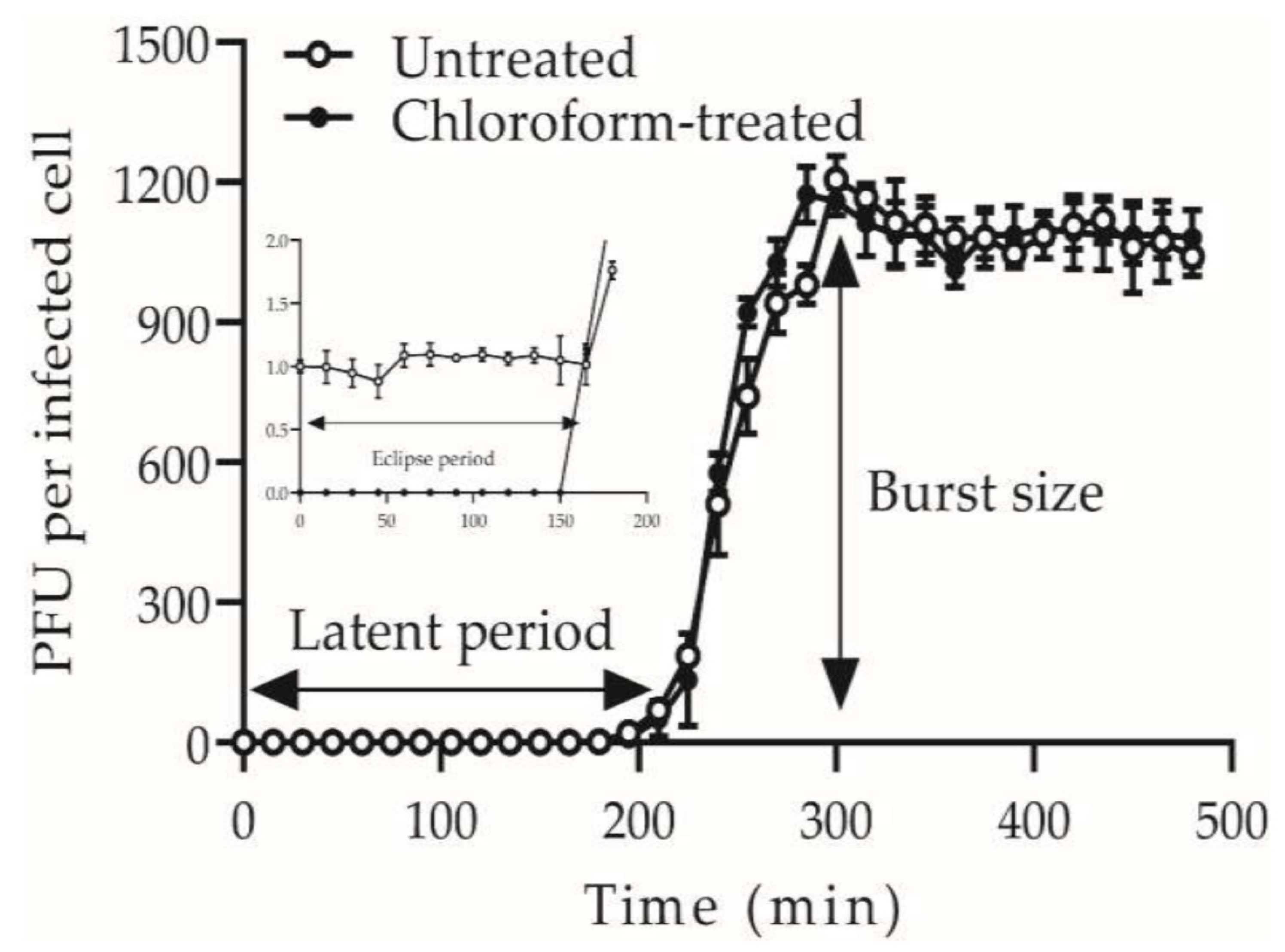
Figure A2.
Ongoing phage adsorption, but to only minimally permissive bacteria? Going from 0 to about 40 min there is an odd, ongoing decline in PFUs/ml. As the y axis shows effectively the log of those PFUs, the straight-line decline is suggestive of a standard phage adsorption curve [6]. Thus, this curve is suggestive of an absence of adsorption synchronization (Section 3.2.3). Note that it is not apparent from the article what OSG protocol was employed. Reported are a constant period of between 55 and 60 minutes and a burst size of 110 [92]. This figure possesses a Creative Commons Attribution License “which permits unrestricted use, distribution, and reproduction in any medium, provided the original author and source are credited.”
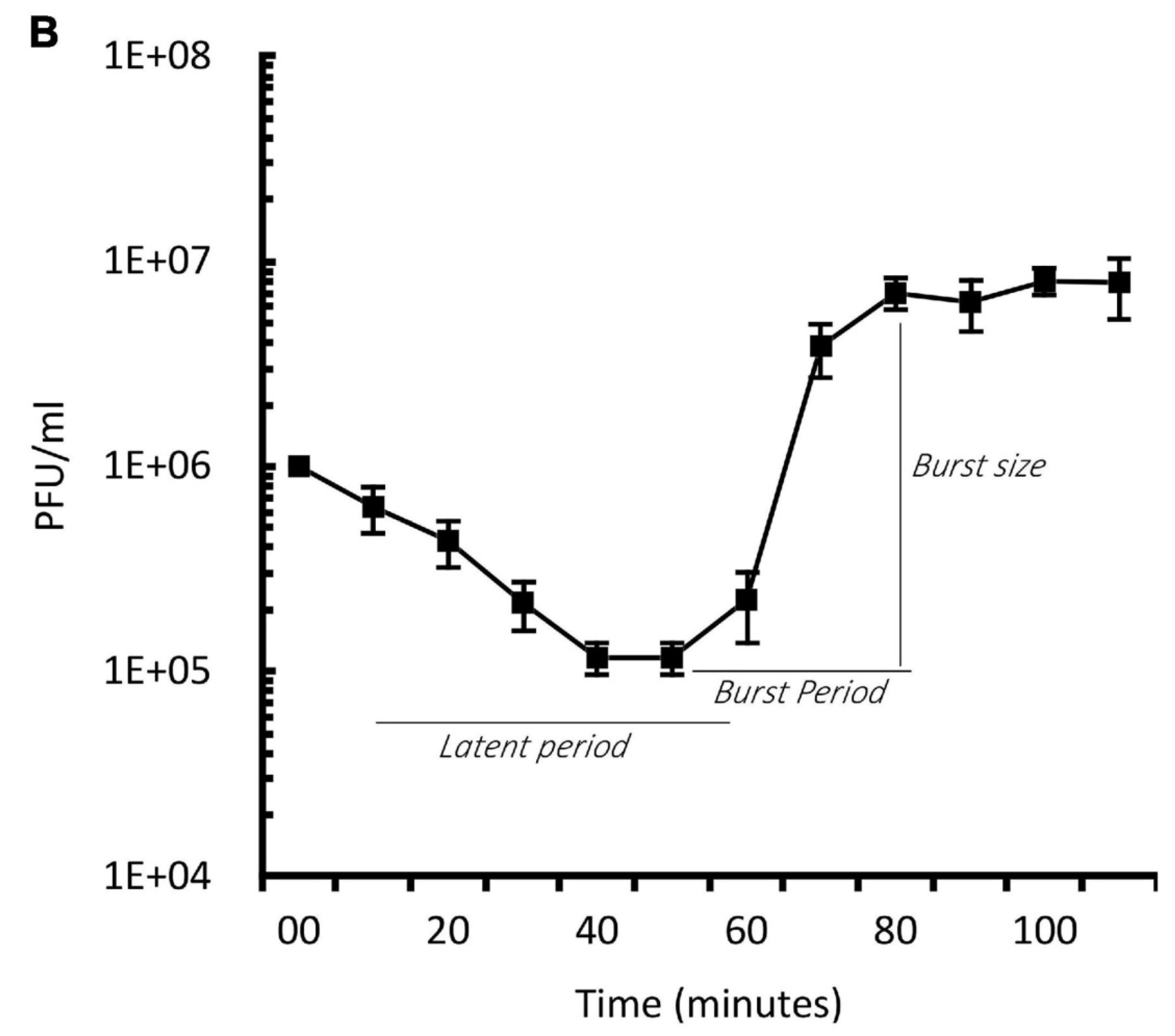
Figure A3.
Application of chloroform indicating ongoing virion adsorption. While free phages usually are not affected by chloroform, phage-infected bacteria are killed and/or lysed by this treatment (Section 5.3). The red-triangle curve thus indicates a continuing, indeed exponential decline in numbers of free phages through until about 30 min, thus suggesting ongoing phage adsorption over that span, i.e., a lack of adsorption synchronization (Section 3.2.3). This curve also lacks sufficient time points taken during the rise (Section 3.4 and Section 3.6.2). The bottoming out of the red-triangle curve between 30 and 50 min is suggestive of a virion cohort that is temporarily not adsorption capable, which can be described as “Residual” [66,93]. Note that the bacterial host (Listeria monocytogenes) was used at a concentration of 109 CFUs/ml and no subsequent diluting is indicated [94], an approach to OSG apparently shared by the publication from which their protocol was obtained [95] (see Section 3.3.4 for more on diluting). Reported are a constant period of between 60 and 70 minutes and a burst size of 11.03 [94]. Also reported is an eclipse (Section 5.3) that ends at 40-50 min, but that value actually should be calculated as closer to 70 min, i.e., the time at which the two graphs first intersect. We can speculate that the small burst size is a consequence of starting with such high bacterial concentrations along with no subsequent culture diluting. This figure possesses a Creative Commons Attribution License “which permits unrestricted use, distribution, and reproduction in any medium, provided the original author and source are credited.”
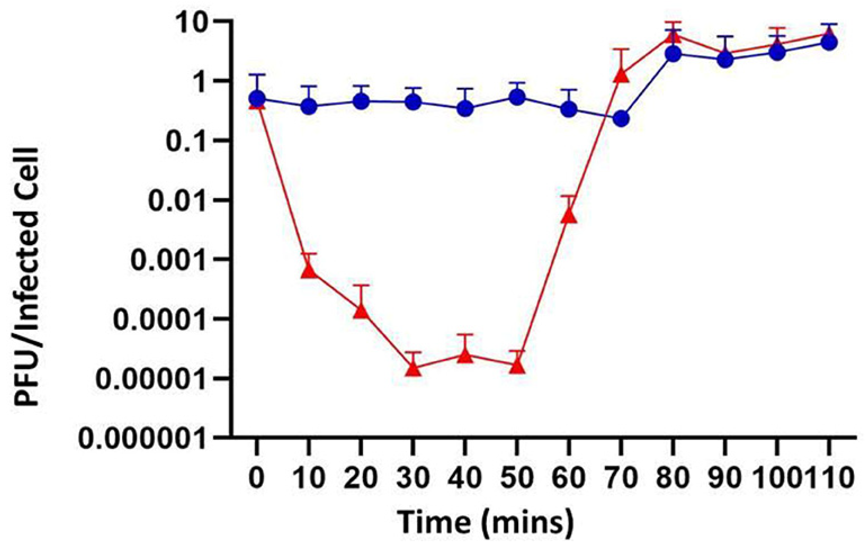
Figure A4.
Intervals between time points are too long. Lysis may have begun around 15 minutes, though it is difficult to tell, other than that it occurred sometime between 10 and 20 minutes. The time points taken at the indicated time zero may or may not have been post-adsorption. The curve fitting, though, is appreciated. Reported are a constant period of 20 minutes, a rise (there, “Burst period”) of 40 min, and a burst size of ~65 [96]. Note that it is difficult to tell how the burst size was calculated from the provided figure, which seems there closer to 500 (= 109.3/106.6) than to 65. These authors do cite Garbe et al. [68] for the OSG protocol (Section 3.5.4.4), but this does not seem to help to explain that discrepancy. This figure possesses a Creative Commons Attribution License “which permits unrestricted use, distribution, and reproduction in any medium, provided the original author and source are credited.”
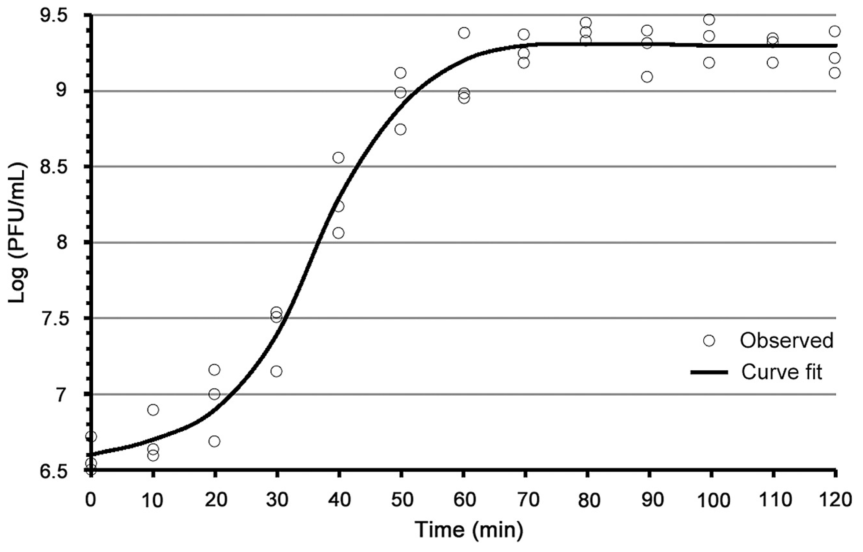
Figure A5.
No post-adsorption period assessed? As this curve begins at zero minutes but has no other pre-lysis time points, it is possible that no actual pre-lysis time points were taken, vs. the zero point being defined as the titer of phages added at the start of the experiment (see perhaps similarly, see Figure 0045246, this appendix). Reported was, “The phage titer increased 10 min after infection and peaked at 30 min, indicating a phage lysis time of approximately 30 min”, implying a constant period of 10 min and a 20-min rise [97]. It is not obvious that any burst size was reported though it looks from the graph to be in the vicinity of 300. This figure possesses a Creative Commons Attribution License “which permits unrestricted use, distribution, and reproduction in any medium, provided the original author and source are credited.”
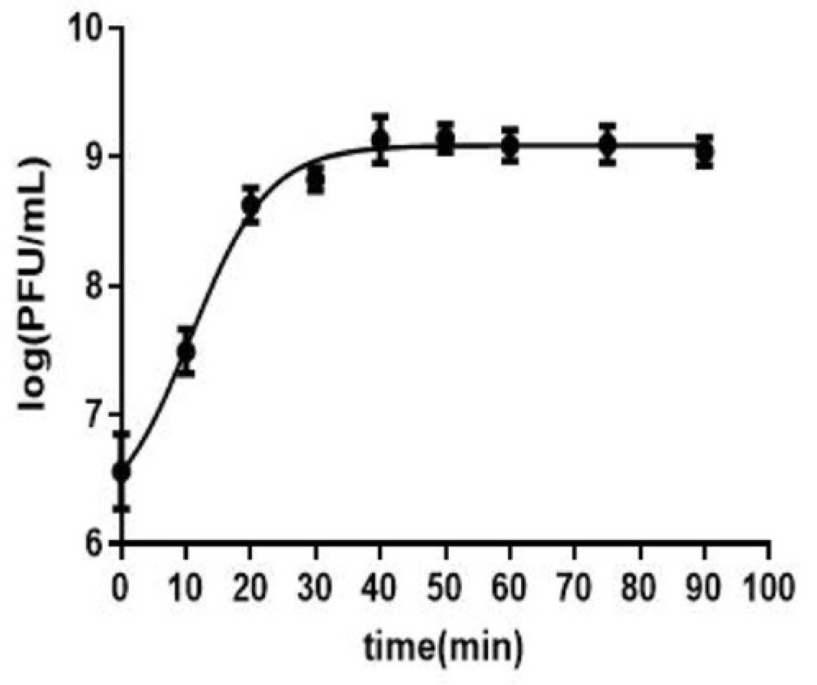
Figure A6.
One-step growth experiment where additional time points before and during the rise could have been useful. The figure is fairly well done including in terms of normalizing the y axis (Section 3.5.3), though note especially for the ATCC 14028 curve the size of the error bars at 45 min as well as post-rise. The experiment could have been improved by increasing the number of time points taken especially between 30 and 50 min, in this case, e.g., by taking 2.5-min rather that 5-min time points over that span. That would have helped especially in better defining the start of the rise, which seems to be at 35 minutes, but is it earlier? Reported are constant periods of 30 min and burst sizes of 130 and 220 [79]. Note though that it is difficult to agree with the 30-min estimate as it seems closer to 35 minutes. This figure possesses a Creative Commons Attribution License “which permits unrestricted use, distribution, and reproduction in any medium, provided the original author and source are credited.”
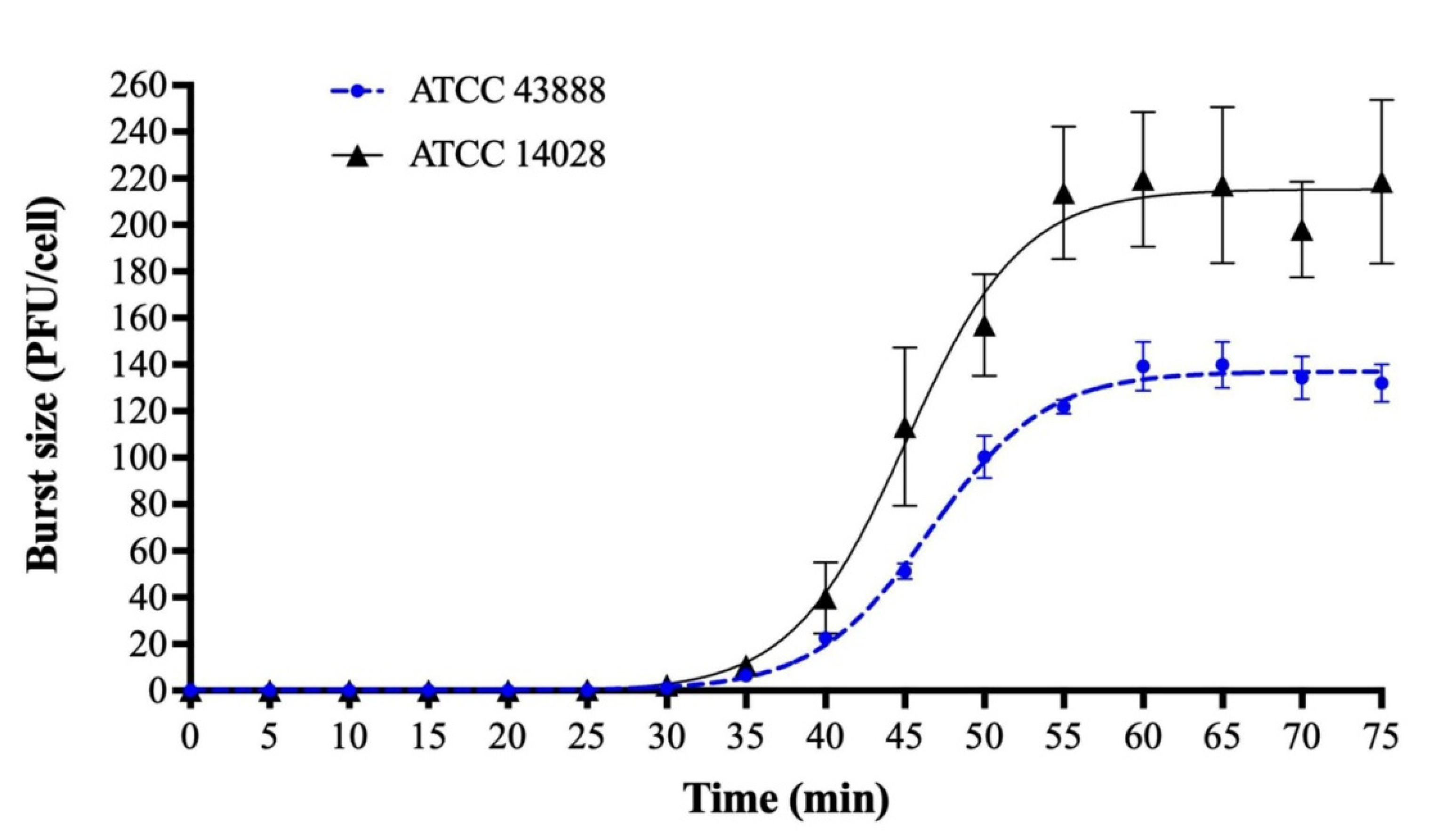
Figure A7.
Varying intervals between time points but not strategically. Missing from this experiment are sufficient numbers of time points taken pre-lysis as well as post-rise (essentially only two time points for both). Reported is a constant period of 10 min and burst size of 328 [98]. Based at least on the first post-lysis time point, it seems instead that the constant period ends between 10 and 20 min (second and third time points). It also is possible that this is a two-step rather than one-step growth curve (Section 3.5.1). There are three pieces of evidence for the latter suggestion. The first is that in their OSG protocol there is no explicit mention of diluting (Section 3.3.4). The second is the long rise relative to a possibly very short constant period. Lastly is the peculiar dip associated with the fourth time point, around 30 min. The latter hypothetically could correspond to a decline in infective centers as phage released from the first round of lysis multiply adsorb individual bacteria, reducing numbers of PFUs even if all phage-infected bacteria remain viable. That titer corresponding to that dip interestingly is about 108 PFUs/ml, a not atypical OSG starting bacterial concentration. This speculation of multi-step growth isn’t necessarily correct, but also in our opinion cannot be ruled out with certainty based on the data presented. This figure possesses a Creative Commons Attribution License “which permits unrestricted use, distribution, and reproduction in any medium, provided the original author and source are credited.”
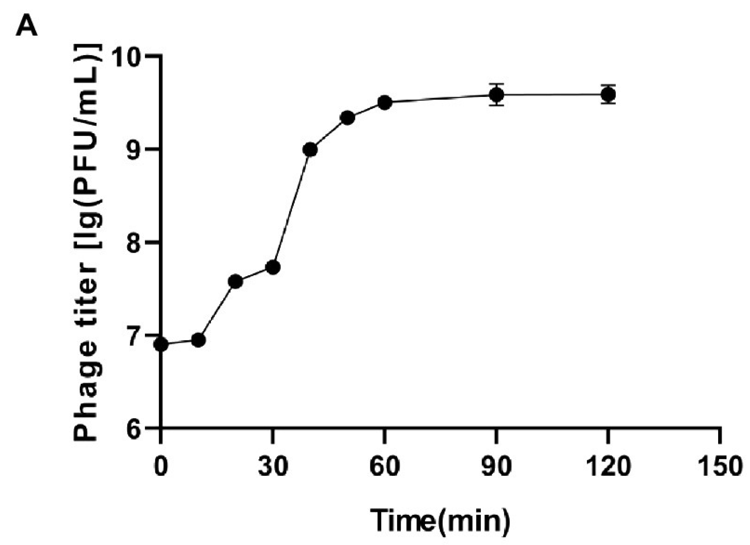
Figure A8.
Taking too few time points. This experiment seems to have used ten-min time points. Note the insufficient number of time points taken prior to lysis as well as during lysis. It is also curious how the y axis is normalized (Section 3.5.3), which does not seem to be to the pre-lysis phage titer. On the other hand, a sufficient number of time points appear to have been taken post-lysis, i.e., starting at 30 minutes. During that time plateauing of those titers, as is expected given a properly performed OSG experiment (Section 3.5.2), is obvious from the figure. It is difficult to say, though, what has been accomplished in this experiment by employing CHCl3 since no obvious eclipse characterization is present (Section 5.3). Reported is a “Generation time” of 30 min and burst size of 142 [99]. Though possibly difficult to appreciate, the reported burst size actually makes sense from the figure as, e.g., 102/10-0.06 = 115, or within the ballpark of the reported burst size based on only rough estimations. Of interest, an MOI of 10 was used (Section 3.2.2), no dilutions of the experimental culture (Section 3.3.4) seem to have been made, and cultures were centrifuged prior to enumeration. Regarding the latter, and though it’s not obvious from the Methods, we speculate that only free phages were being titered throughout the assay, which means that the actual burst size may have been a bit lower than 142, if pre-lysis phage-infected bacteria were not actually being enumerated pre-lysis (a larger pre-lysis titer would mean a smaller calculated burst size; Section 3.5.4). This figure possesses a Creative Commons Attribution License “which permits unrestricted use, distribution, and reproduction in any medium, provided the original author and source are credited.”
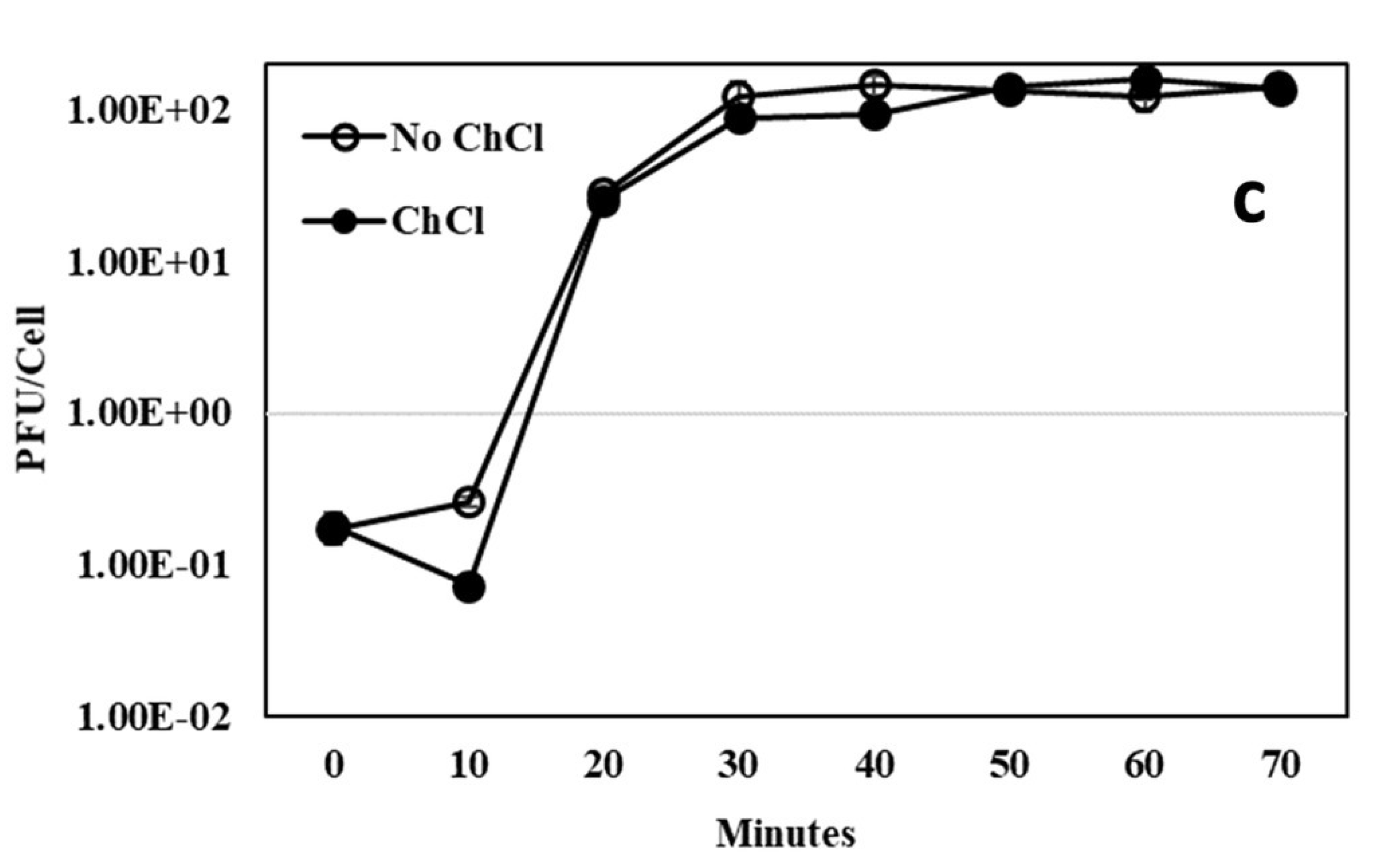
Figure A9.
Gap in time points coinciding with the end of the constant period. The start of the rise thus appears to start somewhere between 6 min and 10 min into the experiment. This figure also would benefit from greater emphasis on the zero- to 20-min portion of the curve where all of the OSG occurred. In addition, better numbering of the x axis would be helpful. Reported are a constant period of 5 min (which would be unusually short), a burst size of 292 (which would be unexpected high given a 5-min constant period), and an end of the rise (“lytic cycle length”) of 20 min [100]. This figure possesses a Creative Commons Attribution License “which permits unrestricted use, distribution, and reproduction in any medium, provided the original author and source are credited.”
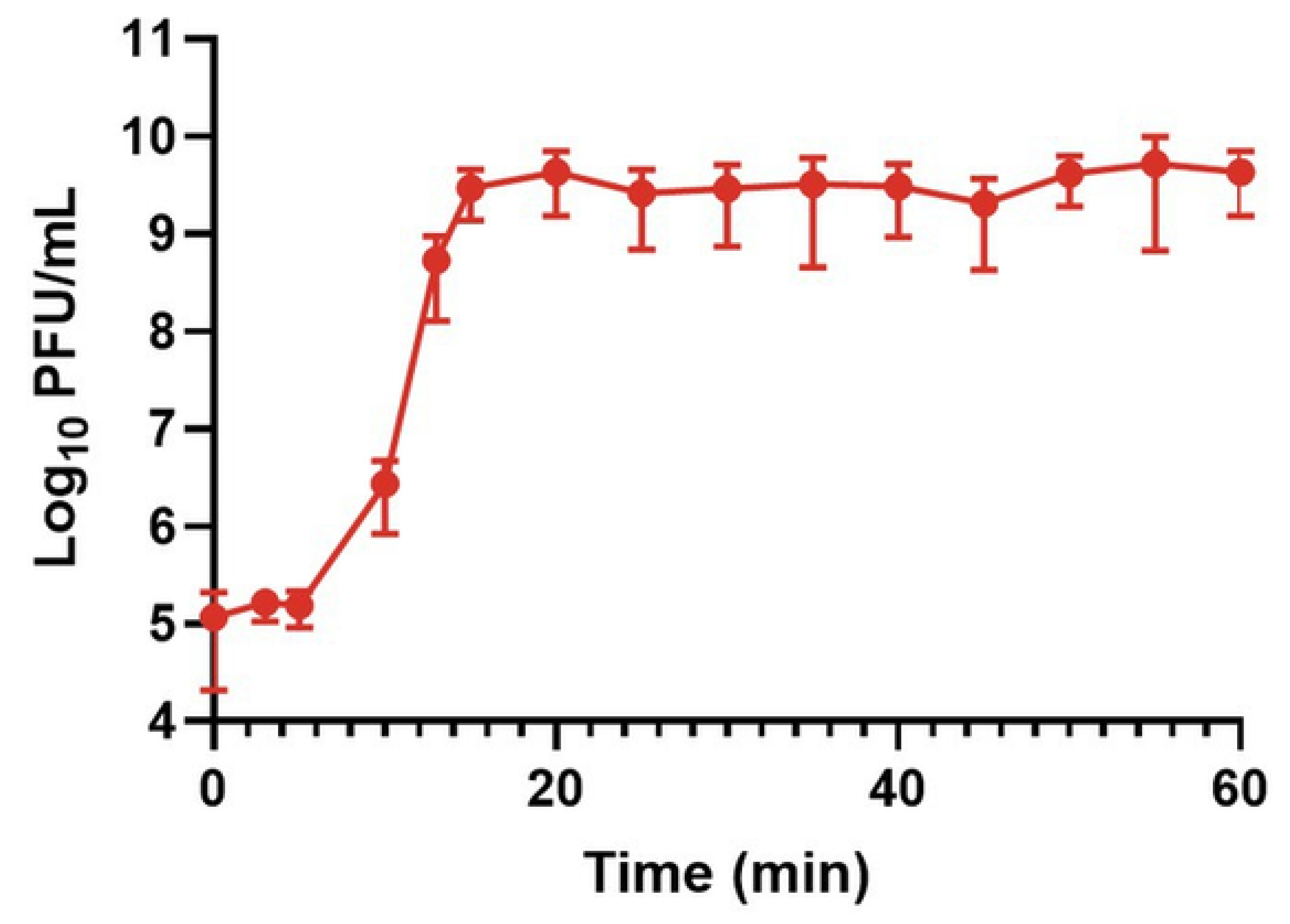
Figure A10.
Too-few time points defining the rise and post-rise. This figure illustrates normalization of the y axis but also: (a) an ongoing rise during the supposed pre-lysis period, (b) only a single time point capturing the majority of the vertical rise, (c) taking only 15-min time points, and (d) too little effort to capture the post-rise. Reported are a constant period of 90 min, along with a burst size of 52 and “Burst periods”/”Burst time” (as synonyms for the rise) of 75 min [101]. Though it is certainly possible that the constant period, i.e., the minimal latent period, indeed is reported correctly, the shape of the reported rise, spanning apparently from roughly 90 min to 150 min is unusual. It is difficult to tell from the OSG protocol why this is so, though we can speculate that it either has something to do with how the infective centers were handled in the course of plating or that this is a phage for which a small minority of infections lyse very early. This figure possesses a Creative Commons Attribution License “which permits unrestricted use, distribution, and reproduction in any medium, provided the original author and source are credited.”
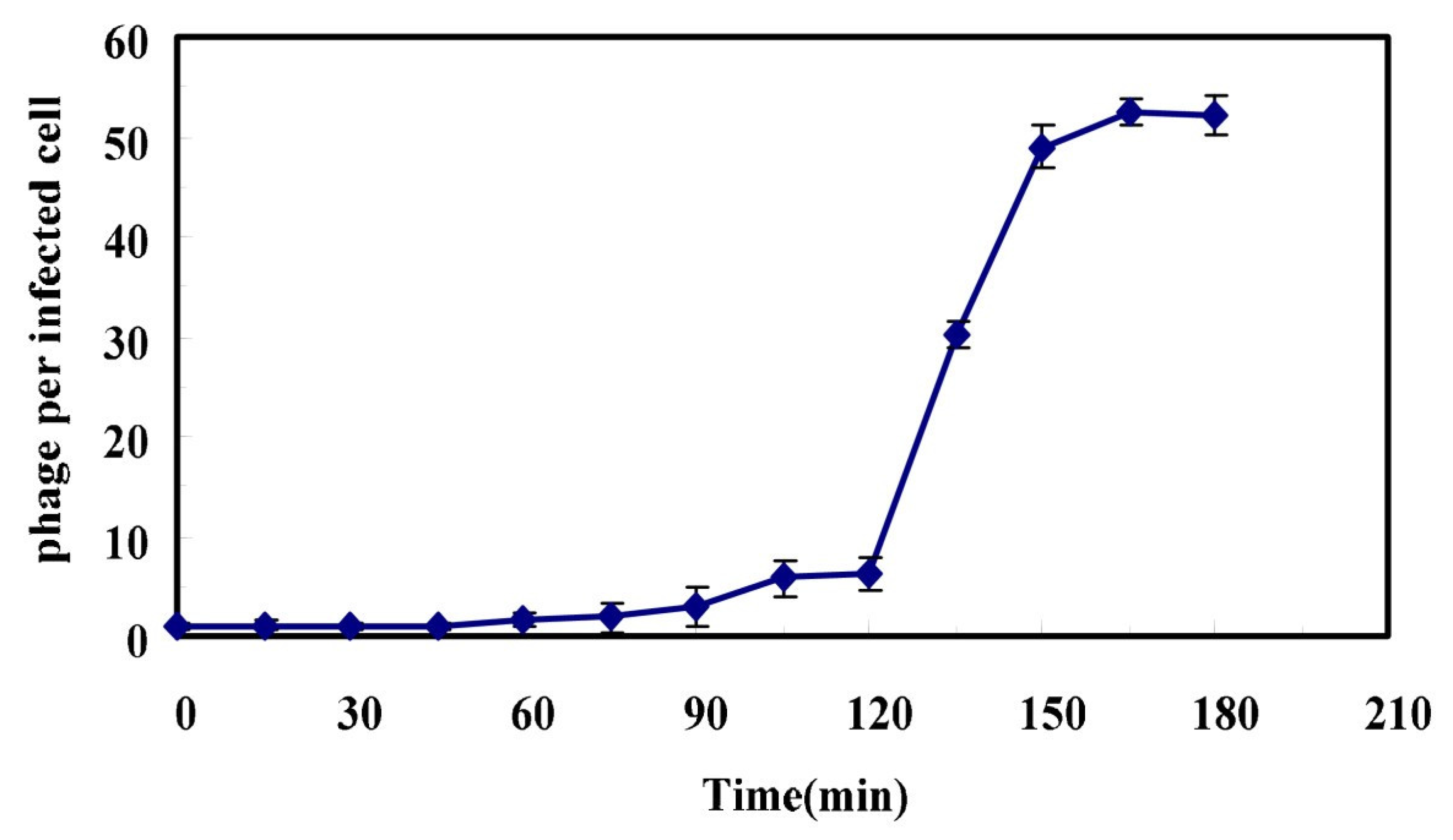
Figure A11.
Another example of too-few time points taken during the rise. The rise seems to begin after 25 min and prior to 30 min, and end after 30 min but prior to 40 min. In addition, note the change of scale on the x axis going from 25 to 30 to 40 minutes. The graph in addition appears to be normalized (Section 3.5.3) but perhaps to the first time point rather than to the average (or equivalent; Section 3.5.4.2) of the pre-lysis titers, which presumably were used to calculate burst size. Also, it would have been preferable to have more post-rise time points (Section 3.5.2), particularly since at that point in the experiments time points were being taken only every ten minutes. Reported are a constant period of 25 minutes and a burst size of 52 [102]. That burst size would seem to be consistent with a normalized, average (or equivalent; Section 3.5.4.2) pre-lysis titer that is greater than the indicated 100 value rather than an average of all of the pre-lysis phage titers. No OSG protocol appears to have been reported. This figure possesses a Creative Commons Attribution License “which permits unrestricted use, distribution, and reproduction in any medium, provided the original author and source are credited.”

Figure A12.
No time points taken during the rise proper? Here, note that from time zero through approaching 40 min the curve rises about two-fold. Then it jumps, relative to time zero about 100-fold. The jump from the two points bracketing the rise, however, is only about 20-fold, from roughly 3 to roughly 60 PFUs/ml. The problem here is that there are approximately ten-min intervals between time points, whereas far more time points were needed during the rise to properly appreciate the observed kinetics. In addition, the small but nonetheless gradual rise occurring seemingly pre-lysis (prior to 40 min) needs to be rigorously addressed since that increase in titers contributes substantial uncertainty as to the burst size determination. Proper dilution and also assessing for unadsorbed phages were both done, though the latter determination of numbers of free phages was done only at the beginning of the assay. An alternative interpretation of the experiment therefore is that lysis began prior to 20 min but that the curve otherwise resembles that of Sun et al. [101] in Figure 0034153, this appendix. Adsorption took place with bacteria on ice, so it is possible that this treatment in some manner resulted in the possibly unusual lysis kinetics observed in this figure. Reported are a constant period of ~40 minutes and a burst size of ~140 [103]. This figure possesses a Creative Commons Attribution License “which permits unrestricted use, distribution, and reproduction in any medium, provided the original author and source are credited.”

Figure A13.
Seemingly well done one-step growth experiment but lacking indication of a post-rise (top figure). Consequently burst size is not calculable. However, in the supplementary materials the more complete OSG experiment is shown (bottom figure). Regardless, note the linearity of the presumed rise in the top figure, even without log transformation of the y axis (Section 3.4.5). Reported is a constant period of 14 min and burst size of 13 [104]. We otherwise are unable to interpret this experiment as OSG. However, there is no mention of diluting in the Methods of this study, so it is possible that what is being observed here is multi-step growth (Section 3.5.1). This figure possesses a Creative Commons Attribution License “which permits unrestricted use, distribution, and reproduction in any medium, provided the original author and source are credited.”

Figure A14.
Definitive multi-step growth? Note the 1,000-fold-plus increase in phage titer before plateauing, as occurs over a 50-min time span. Reported is a constant period of “Short” minute’s long and burst size of 110 [105]. The use of “Short” presumably is to suggest that the constant period ended prior to 10 min. The bust size claim is difficult to understand as 1010/106.5 ≈ 3,000. It is possible, therefore, that what is being observed is multi-step growth (Section 3.5.1). Consistently, no culture dilution (Section 3.3.4) is indicated in the supplied OSG protocol. This figure possesses a Creative Commons Attribution License “which permits unrestricted use, distribution, and reproduction in any medium, provided the original author and source are credited.”
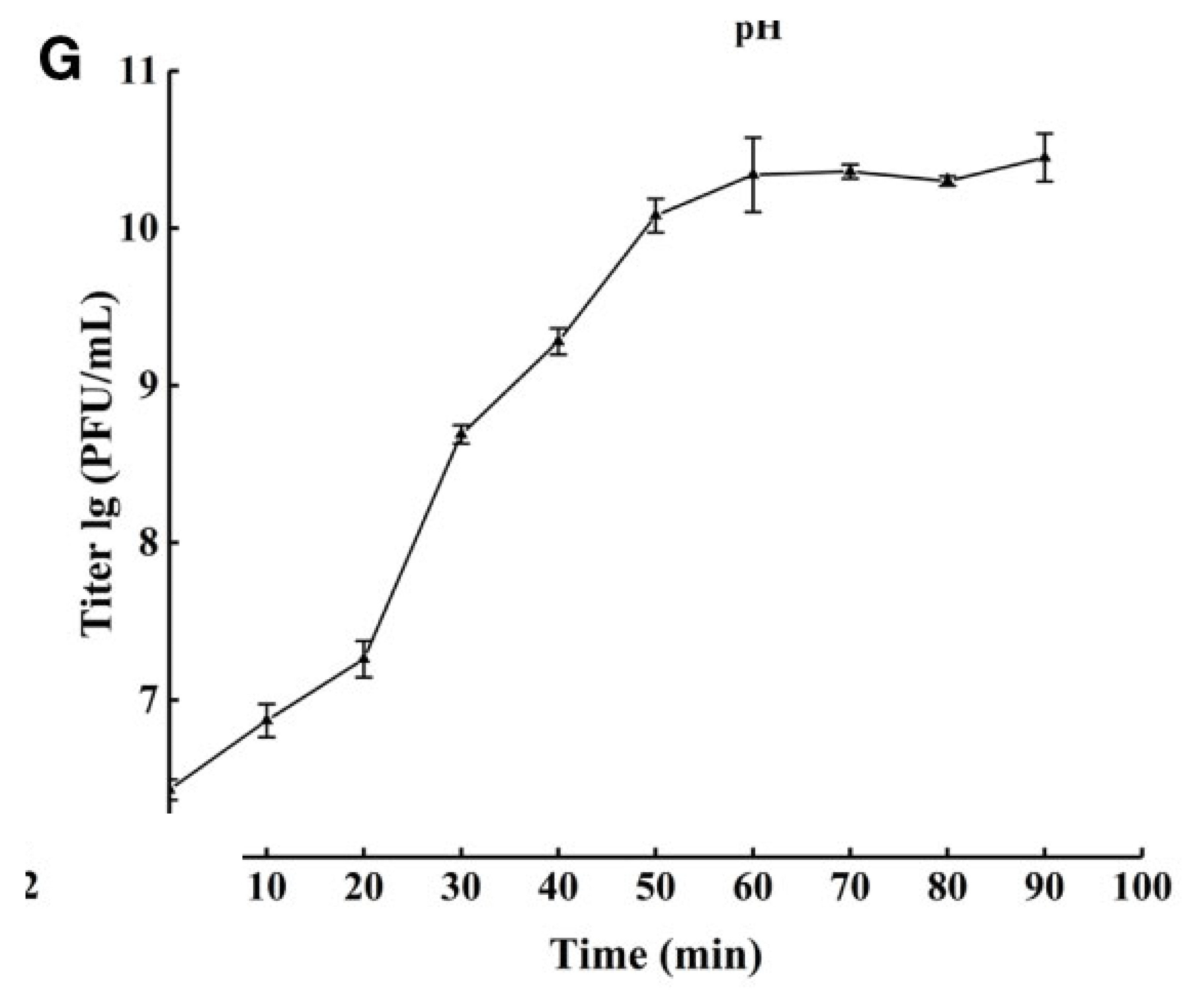
Figure A15.
Another relatively large burst size in combination with a poorly defined end of the constant period. It also is odd in particular that phage titer seems to have increased two-fold over the first five minutes of the experiment. It appears that the culture was diluted perhaps 50-fold following adsorption. That should be viewed at best as a barely adequate amount of dilution (Section 3.3.4) and it is difficult to say what the starting bacterial concentration was. If we assume that it was 108 CFUs/ml, then a 50-fold dilution would reduce the bacterial concentration to 2 × 10⁶ CFUs/ml. The starting MOI was a reported 0.001, implying a starting titer of 105 PFUs/ml, which is what is indicated here. Reported is a constant period of 10 min and burst size of 378 [106]. This figure possesses a Creative Commons Attribution License “which permits unrestricted use, distribution, and reproduction in any medium, provided the original author and source are credited.”
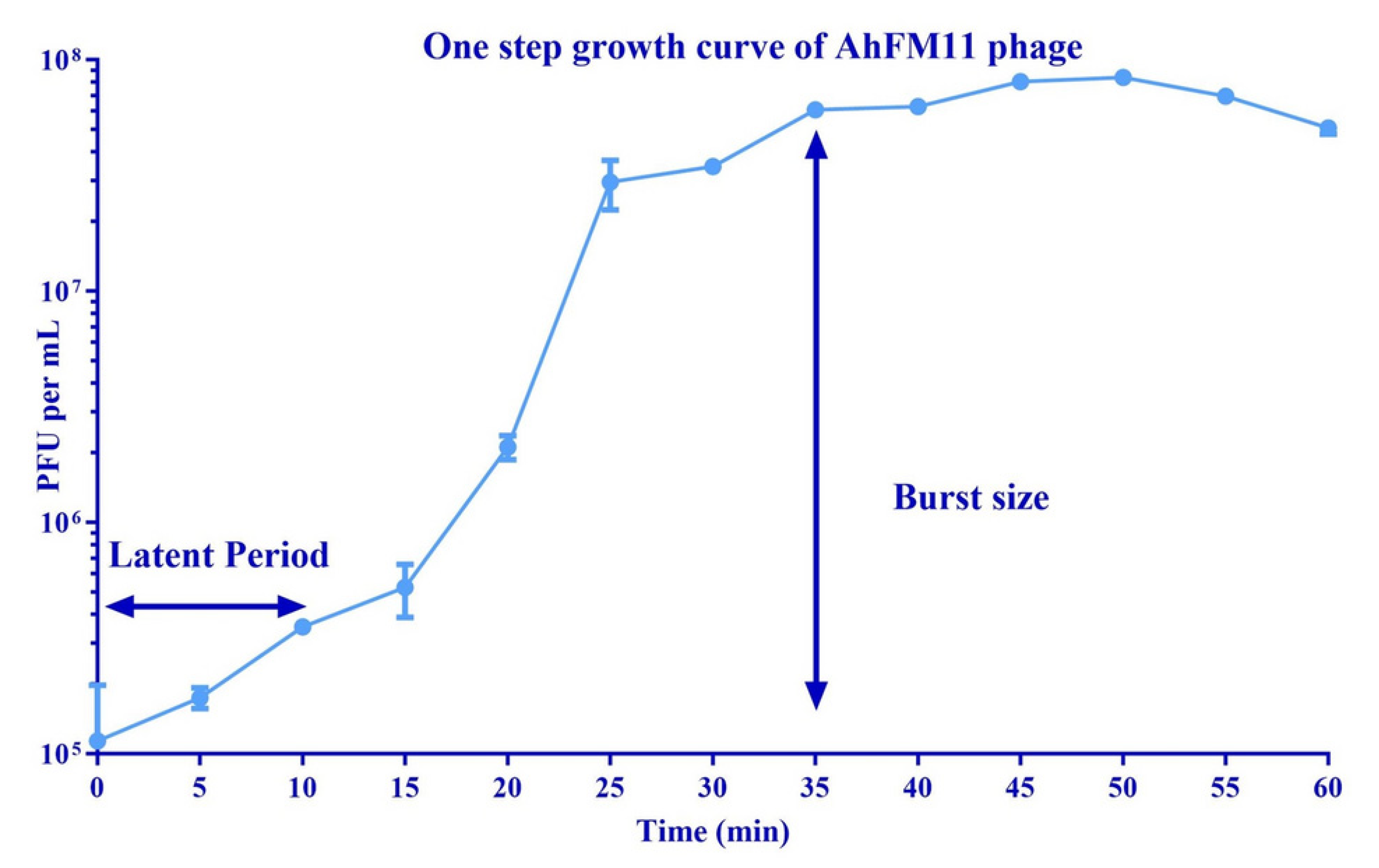
Figure A16.
Another example of possible multi-step growth. Reported are a constant period of 10 minutes and a burst size of 38 [102]. This seems to suggest a post-lysis, pre-multi-step period spanning 20 and 25 min (a kind of temporary post-rise plateauing; Section 3.5.2; and not also the huge variation at t = 30), though that in turn would suggest a burst size of closer to 100. Therefore, it seems likely that the time point at 15 min, only, was used to calculate burst size. No OSG protocol appears to be reported, though we speculate that insufficient experimental culture dilution was involved (Section 3.3.4). This figure possesses a Creative Commons Attribution License “which permits unrestricted use, distribution, and reproduction in any medium, provided the original author and source are credited.”
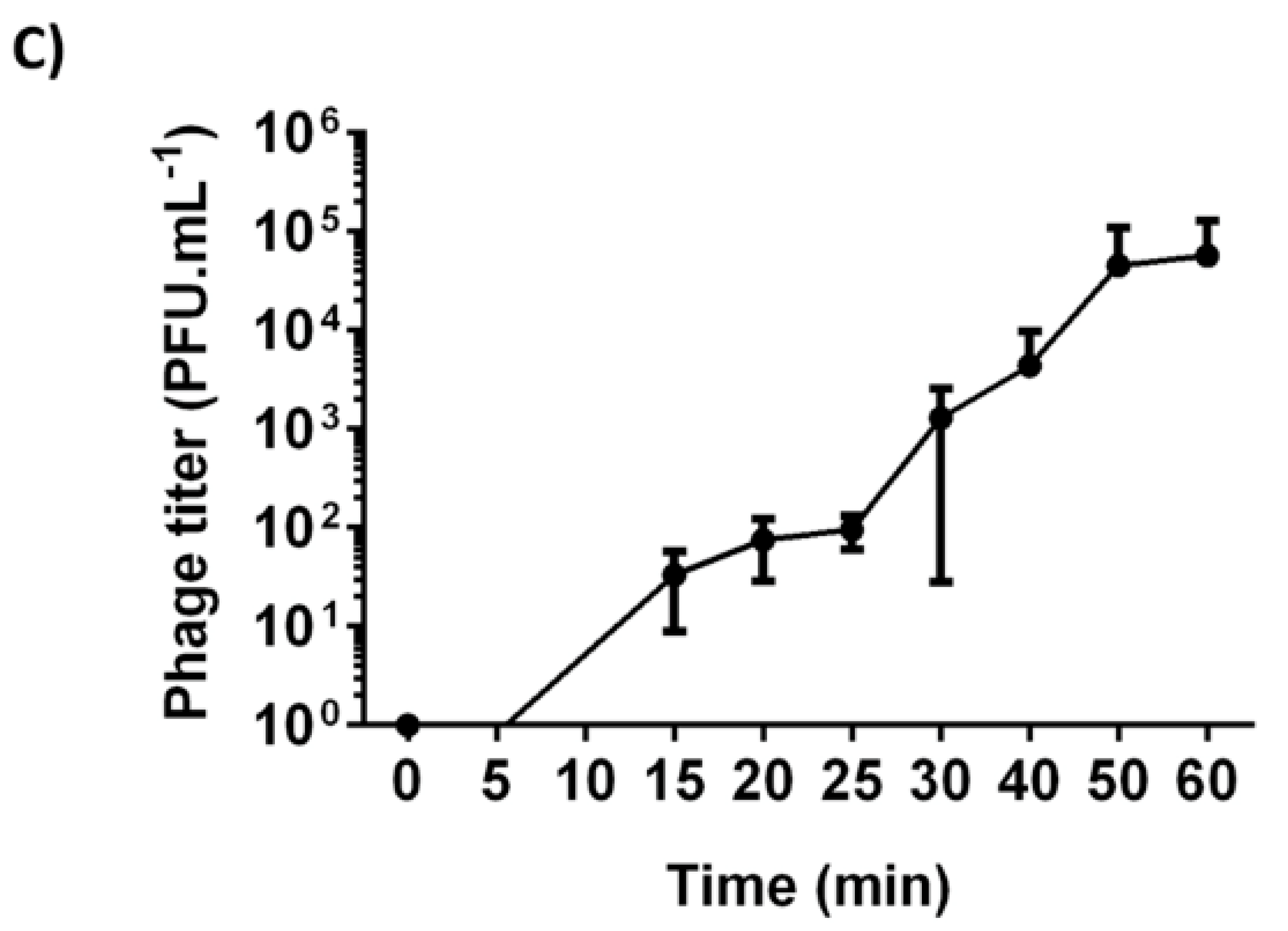
Figure A17.
Another example of possible multi-step growth, or just a very long rise? Reported is a constant period of 10 min and burst size of 120 [107]. Of course, the constant period really should be indicated as less than 20 but more than 10 min. The rise appears to be very long (a “Burst period” of 50 min), hence the concern over whether this is another example of multi-step growth (Section 3.5.1). That concern is compounded because no dilutions of the experimental culture (Section 3.3.4) are reported in the Methods section. This figure possesses a Creative Commons Attribution License “which permits unrestricted use, distribution, and reproduction in any medium, provided the original author and source are credited.”

Figure A18.
Illustration of possible multi-step growth. Superficially, this seems to be indicated by the bump in titer at the last time point. That increase, though, actually is relatively slight. Instead, it is possible that the multi-step growth actually commenced after the indicated 20-min time point. Perhaps supporting that interpretation, note the y axis which starts at 106 PFUs/ml, then jumps to 5 × 10⁸ PFUs/ml (a 500-fold increase), and then with same spacing increases two-fold or 100%. The next step increases by 50%, and so on. This suggests a much larger increase in titer between 20 and 30 min than the graph at first glance would seem to illustrate. Alternatively, the increase from 40 min to 55 min may be less than ten-fold. Another issue is whether that last time point was taken into account when calculating the post-lysis titer. Indeed, as indicated, the actual burst size seems to be approximately 2,000 phages/cell, going from approximately 106 PFUs/ml to approximately 2 × 10⁹ PFUs/ml. Supporting the possibility that this is multi-step growth that is being observed, the protocol used does not seem to include dilution of the experimental culture (Section 3.3.4). Reported is a constant period of 20 min and burst size of 210 [77]. As noted, it is difficult to tell from the graph what the reported burst size has been calculated from. This figure possesses a Creative Commons Attribution License “which permits unrestricted use, distribution, and reproduction in any medium, provided the original author and source are credited.”..
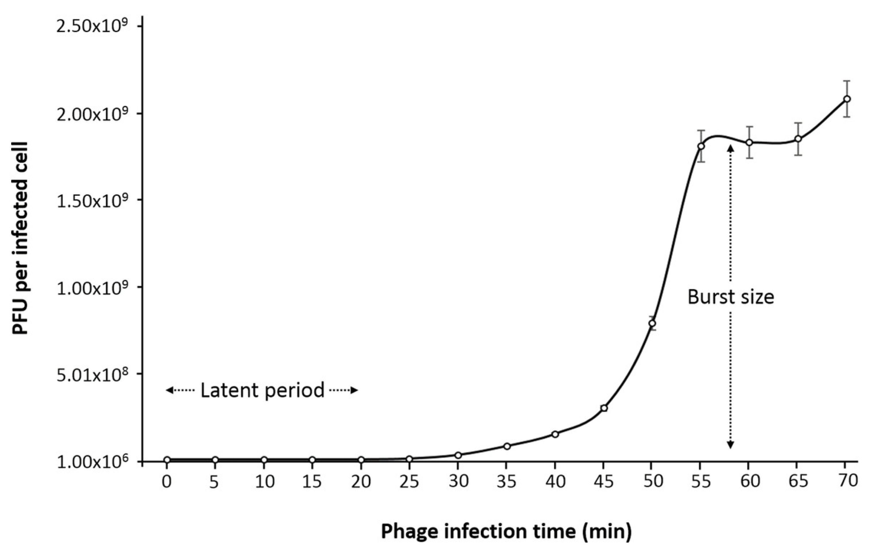
Figure A19.
Illustration of assessing plateauing using common computer tools. In this case a rectangle shape was inserted which was then formatted so that it had relatively little opaque fill. Reported is a constant period of 35 min and burst size of 316 [108]. Note the gradual rise of both the pre-lysis and post-rise periods. No dilution of the experimental cultures is indicated (Section 3.3.4) though it is possible that this occurred since otherwise nearly 20 100 μl volumes would need to have been removed from a described single ml of culture. Note that this study also supplies a second OSG experiment using a different phage though with similar pre-lysis and post-rise increases in phage titers. This figure possesses a Creative Commons Attribution License “which permits unrestricted use, distribution, and reproduction in any medium, provided the original author and source are credited.”
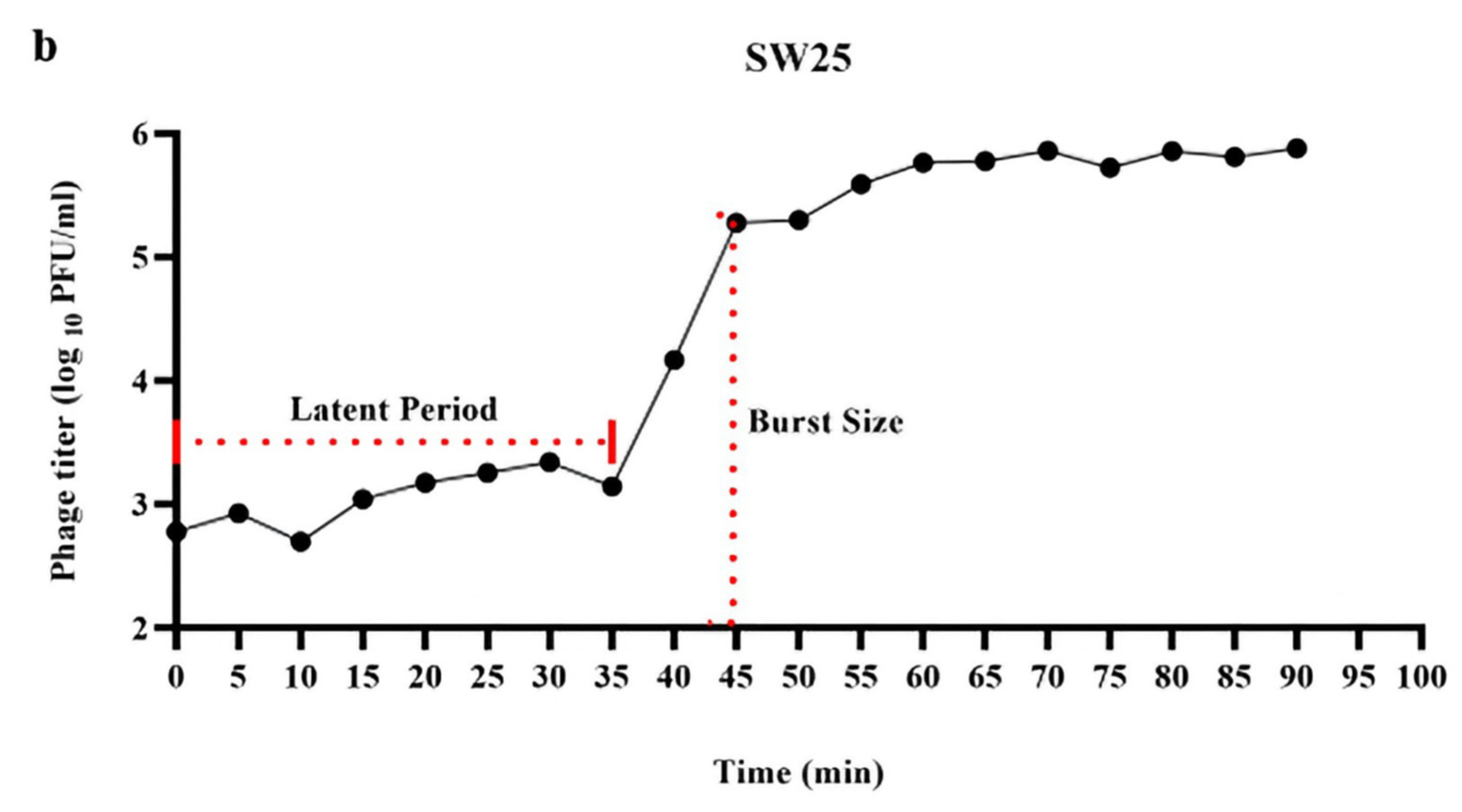
Figure A20.
Possible insufficient diluting as well as lack of post-rise plateauing. Reported is a constant period of 20 min and burst size of 174 [109]. That burst size also seems to have been calculated based solely on the time = zero point as the denominator.
Figure A20.
Possible insufficient diluting as well as lack of post-rise plateauing. Reported is a constant period of 20 min and burst size of 174 [109]. That burst size also seems to have been calculated based solely on the time = zero point as the denominator.
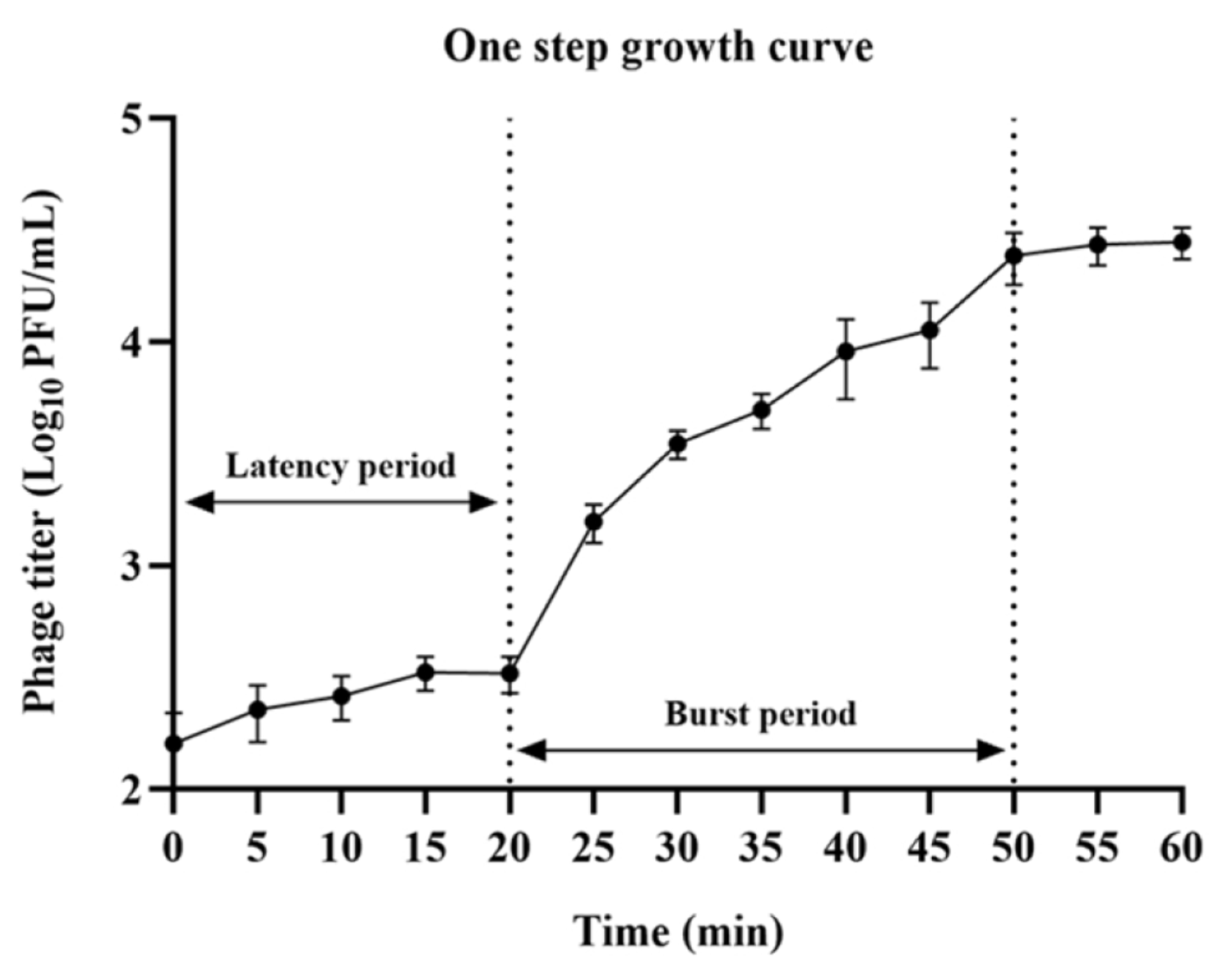
Figure A21.
Assessing burst sizes by eye. Ideally from OSG figures it will be possible at a glance to confirm reported burst sizes. This can be most easily accomplished by normalizing titers to average (or equivalent; Section 3.5.4.2) pre-lysis phage titers (Section 3.5.3). In this figure, that appears to be what has been done. Ideally as well the y axis would have been log-transformed. That accomplishes two useful things. First, it places the average (or equivalent; Section 3.5.4.2) pre-lysis titer explicitly on an identifiable value of 1. The second is that by log-transforming the y axis, it becomes possible to much more easily visually assess the amount of variation in titers seen prior to lysis; e.g., no variation is visible pre-lysis in the figure. This issue of not log transforming the y axis and not being able to see pre-lysis variance can also be seen in Figures 0045241, 0045247 and 0034153. Note that to view this pre-lysis variation, it is essential for y axes to start below 1, such as with 0.1, though that value need not be that low, just so long as all of the pre-lysis data points are properly graphed. In this graph, the y axis instead falls below zero, but since data points won’t fall below zero, that is being done here solely for aesthetic reasons. Reported is a constant period of 40 min and burst size of 400, the latter for the untreated culture [110]. This figure possesses a Creative Commons Attribution License “which permits unrestricted use, distribution, and reproduction in any medium, provided the original author and source are credited.”

References
- Adams, M. H. Bacteriophages; InterScience: New York, 1959.
- Ellis, E. L.; Delbrück, M. The growth of bacteriophage. J. Gen. Physiol. 1939, 22, 365-384. [CrossRef]
- Benzer, S.; Hudson, W.; Weidel, W.; Delbrück, M.; Stent, G. S.; Weigle, J. J.; Dulbecco, R.; Watson, J. D.; Wollman, E. L. A syllabus on procedures, facts, and interpretations in phage. In Viruses 1950, Delbrück, M., Ed.; California Institute of Technology: Pasadena, CA, 1950; 100-147.
- Stent, G. S. Molecular Biology of Bacterial Viruses; WH Freeman and Co.: San Francisco, CA, 1963.
- Carlson, K. Single-step growth. In Molecular Biology of Bacteriophage T4, Karam, J. D., Ed.; ASM Press: Washington, 1994; 434-437.
- Hyman, P.; Abedon, S. T. Practical methods for determining phage growth parameters. Meth. Mol. Biol. 2009, 501, 175-202. [CrossRef]
- Kropinski, A. M. Practical advice on the one-step growth curve. Meth. Mol. Biol. 2018, 1681, 41-47. [CrossRef]
- Adams, M. H. Mixed infection with bacterial virus T5 and its heat stable mutant. J. Immunol. 1951, 66, 131-136. [CrossRef]
- Summers, W. C. Bacteriophage research: early research. In Bacteriophages: Biology and Application, Kutter, E.; Sulakvelidze, A., Eds.; CRC Press: Boca Raton, Florida, 2005; 5-28.
- Sankaran, N. Stepping-stones to one-step growth: Frank Macfarlane Burnet’s role in elucidating the viral nature of the bacteriophages. Historical Records of Australian Science 2008, 19, 83-100. [CrossRef]
- Dennehy, J. J.; Abedon, S. T. Phage infection and lysis. In Bacteriophages: Biology, Technology, Therapy, Harper, D., Abedon, S. T., Burrowes, B. H.; McConville, M., Eds.; Springer Nature Switzerland AG: New York City, 2021; 341-383.
- Abedon, S. T. Evolution of bacteriophage latent period length. In Evolutionary Biology: New Perspectives on its Development, Dickins, T. E.; Dickens, B. J. A., Eds.; Springer: Cham, Switzerland, 2023; 375-426.
- Dennehy, J. J.; Abedon, S. T. Adsorption: phage acquisition of bacteria. In Bacteriophages: Biology, Technology, Therapy, Harper, D., Abedon, S. T., Burrowes, B. H.; McConville, M., Eds.; Springer Nature Switzerland AG: New York City, 2021; 93-117.
- Górski, A.; Miedzybrodzki, R.; Borysowski, J. Phage Therapy: A Practical Approach; Springer Nature: Cham, Switzerland, 2019.
- Abedon, S. T.; Danis-Wlodarczyk, K.; Alves, D. R. Phage therapy in the 21st Century: is there modern, clinical evidence of phage-mediated clinical efficacy? Pharmaceuticals 2021, 14, 1157.
- Marongiu, L.; Burkard, M.; Lauer, U. M.; Hoelzle, L. E.; Venturelli, S. Reassessment of historical clinical trials supports the effectiveness of phage therapy. Clin. Microbiol Rev. 2022, 35, e0006222. [CrossRef]
- Suh, G. A.; Lodise, T. P.; Tamma, P. D.; Knisely, J. M.; Alexander, J.; Aslam, S.; Barton, K. D.; Bizzell, E.; Totten, K. M. C.; Campbell, J.; Chan, B. K.; Cunningham, S. A.; Goodman, K. E.; Greenwood-Quaintance, K.; Harris, A. D.; Hesse, S.; Maresso, A.; Nussenblatt, V.; Pride, D.; Rybak, M.; Sund, Z.; van Duin, D.; Van Tyne, D.; Patel, R. Considerations for the use of phage therapy in clinical practice. Antimicrob. Agents Chemother. 2022, 66, AAC0207121.
- Petrovic Fabijan, A.; Iredell, J.; Danis-Wlodarczyk, K.; Kebriaei, R.; Abedon, S. T. Translating phage therapy into the clinic: recent accomplishments but continuing challenges. PLoS Biol. 2023, 21, e3002119. [CrossRef]
- Strathdee, S. A.; Hatfull, G. F.; Mutalik, V. K.; Schooley, R. T. Phage therapy: From biological mechanisms to future directions. Cell 2023, 186, 17-31. [CrossRef]
- Danis-Wlodarczyk, K.; Alves, D.; Abedon, S. T. Phage therapy: a clinician’s guide. In Handbook of Molecular Biology, Liu, D., Ed.; CRC Press: Boca Raton, FL, 2024.
- Kim, M. K.; Suh, G. A.; Cullen, G. D.; Perez, R. S.; Dharmaraj, T.; Chang, T. H. W.; Li, Z.; Chen, Q.; Green, S. I.; Lavigne, R.; Pirnay, J. P.; Bollyky, P. L.; Sacher, J. C. Bacteriophage therapy for multidrug-resistant infections: current technologies and therapeutic approaches. J Clin. Invest 2025, 135. [CrossRef]
- Dennehy, J. J.; Abedon, S. T. Bacteriophage ecology. In Bacteriophages: Biology, Technology, Therapy, Harper, D., Abedon, S. T., Burrowes, B. H.; McConville, M., Eds.; Springer Nature Switzerland AG: New York City, 2021; 253-294.
- Abedon, S. T. Bacteriophages as Drivers of Evolution: An Evolutionary Ecological Perspective; Springer: Cham, Switzerland, 2022.
- Abedon, S.T. Phage adsorption theory. 2017. https://adsorption.phage.org.
- Abedon, S.T. Phage adsorptions calculator. 2022. https://phage-therapy.org/calculators/adsorptions.html.
- Abedon, S. T. Bacteriophage adsorption: likelihood of virion encounter with bacteria and other factors affecting rates. Antibiotics 2023, 12, 723.
- Antani, J. D.; Ward, T.; Emonet, T.; Turner, P. E. Microscopic phage adsorption assay: high-throughput quantification of virus particle attachment to host bacterial cells. Proc. Natl. Acad. Sci. U. S. A 2024, 121, e2410905121. [CrossRef]
- de Paepe, M.; Taddei, F. Viruses’ life history: towards a mechanistic basis of a trade-off between survival and reproduction among phages. PLoS Biol. 2006, 4, e193.
- Heineman, R. H.; Brown, S. P. Experimental evolution of a bacteriophage virus reveals the trajectory of adaptation across a fecundity/longevity trade-off. PLoS One 2012, 7, e46322.
- Garcia-Villada, L.; Drake, J. W. Experimental selection reveals a trade-off between fecundity and lifespan in the coliphage Qb. Open. Biol. 2013, 3, 130043.
- Payne, R. J. H.; Jansen, V. A. A. Phage therapy: The peculiar kinetics of self-replicating pharmaceuticals. Clin. Pharmacol. Ther. 2000, 68, 225-230. [CrossRef]
- Abedon, S. T.; Thomas-Abedon, C. Phage therapy pharmacology. Curr. Pharm. Biotechnol. 2010, 11, 28-47. [CrossRef]
- Chan, B. K.; Abedon, S. T. Bacteriophage adaptation, with particular attention to issues of phage host range. In Bacteriophages in Dairy Processing, Quiberoni, A.; Reinheimer, J., Eds.; Nova Science Publishers: Hauppauge, New York, 2012; 25-52.
- Weitz, J. S.; Li, G.; Gulbudak, H.; Cortez, M. H.; Whitaker, R. J. Viral invasion fitness across a continuum from lysis to latency. Virus Evol. 2019, 5, vez006.
- Hyman, P.; Abedon, S. T. Bacteriophage host range and bacterial resistance. Adv. Appl. Microbiol. 2010, 70, 217-248.
- Koskella, B.; Meaden, S. Understanding bacteriophage specificity in natural microbial communities. Viruses 2013, 5, 806-823.
- Dabrowska, K.; Abedon, S. T. Pharmacologically aware phage therapy: pharmacodynamic and pharmacokinetic obstacles to phage antibacterial action in animal and human bodies. Microbiol. Mol. Biol. Rev. 2019, 83, e00012-19. [CrossRef]
- Gencay, Y. E.; Gambino, M.; From, P. T.; Brondsted, L. The genera of bacteriophages and their receptors are the major determinants of host range. Environ. Microbiol. 2019, 21, 2095-2111. [CrossRef]
- Hyman, P. Phages for phage therapy: isolation, characterization, and host range breadth. Pharmaceuticals 2019, 12, 35.
- Abedon, S. T.; Danis-Wlodarczyk, K. M.; Wozniak, D. J. Phage cocktail development for bacteriophage therapy: toward improving spectrum of activity breadth and depth. Pharmaceuticals 2021, 14, 1019. [CrossRef]
- Lamy-Besnier, Q.; Brancotte, B.; Menager, H.; Debarbieux, L. Viral Host Range database, an online tool for recording, analyzing and disseminating virus-host interactions. Bioinformatics 2021, 60, 921-925.
- Middelboe, M.; Chan, A.M.; Bertelsen, S.K. One-step growth experiments (bacteriophages). 2016. [CrossRef]
- Kutter, E. Phage host range and efficiency of plating. Meth. Mol. Biol. 2009, 501, 141-149.
- Letarov, A. V.; Kulikov, E. E. Determination of the bacteriophage host range: culture-based approach. Meth. Mol. Biol. 2018, 1693, 75-84.
- Hadas, H.; Einav, M.; Fishov, I.; Zaritsky, A. Bacteriophage T4 development depends on the physiology of its host Escherichia coli. Microbiology 1997, 143, 179-185. [CrossRef]
- Carlson, K. Working with bacteriophages: common techniques and methodological approaches. In Bacteriophages: Biology and Application, Kutter, E.; Sulakvelidze, A., Eds.; CRC Press: Boca Raton, Florida, 2005; 437-494.
- Lanni, F. Small reversible clumps of bacteriophage and their anomalous serologic behavior. J. Immunol. 1959, 83, 148-166.
- Abedon, S. T. Phage therapy dosing: the problem(s) with multiplicity of infection (MOI). Bacteriophage 2016, 6, e1220348. [CrossRef]
- Abedon, S. T. Multiplicity of infection. In Reference Module in Life Sciences, Elsevier: 2017.
- Abedon, S.T. Multiplicity of infection calculator. 2017. https://moicalculator.phage.org.
- Abedon, S. T. Look who’s talking: T-even phage lysis inhibition, the granddaddy of virus-virus intercellular communication research. Viruses 2019, 11, 951. [CrossRef]
- Abedon, S. T. How simple maths can inform our basic understanding of phage therapy. Clin. Infect. Dis. 2023, 77, S401-S406.
- Abedon, S. T.; Katsaounis, T. I. Basic phage mathematics. Meth. Mol. Biol. 2018, 1681, 3-30.
- Abedon, S.T. Poisson frequencies calculator. 2022. https://www.phage.org/calculators/Poisson.html.
- Abedon, S. T. Further considerations on how to improve phage therapy experimentation, practice, and reporting: pharmacodynamics perspectives. Phage 2022, 3, 98-111.
- Abedon, S. T. Automating predictive phage therapy pharmacology. Antibiotics (Basel) 2023, 12, 1423.
- Gadagkar, R.; Gopinathan, K. P. Bacteriophage burst size during multiple infections. J. Biosci. 1980, 2, 253-259. [CrossRef]
- Wedd, C.; Yunusov, T.; Smith, A.; Li, R.; Hardo, G.; Hunter, M.; Majed, R.; Fusco, D.; Bakshi, S. Single-cell imaging of the lytic phage life cycle in bacteria. bioRxiv 2024, 2024-04.
- Delbrück, M. The burst size distribution in the growth of bacterial viruses (bacteriophages). J. Bacteriol. 1945, 50, 131-135.
- Abedon, S. T.; Danis-Wlodarczyk, K. M.; Wozniak, D. J.; Sullivan, M. B. Improving phage-biofilm in vitro experimentation. Viruses 2021, 13, 1175. [CrossRef]
- Doermann, A. H. Intracellular phage growth as studied by premature lysis. Federation Proc. 1951, 10, 591-594.
- Anderson, T. F.; Doermann, A. H. The intracellular growth of bacteriophages. II. The growth of T3 studied by sonic disintegration and by T6-cyanide lysis of infected cell. J. Gen. Physiol. 1952, 35, 657-667.
- Abedon, S. T.; Katsaounis, T. I. Detection of bacteriophages: statistical aspects of plaque assay. In Bacteriophages: Biology, Technology, Therapy, Harper, D., Abedon, S. T., Burrowes, B. H.; McConville, M., Eds.; Springer Nature Switzerland AG: New York City, 2021; 539-560.
- Jongenburger, I.; Reij, M. W.; Boer, E. P.; Gorris, L. G.; Zwietering, M. H. Factors influencing the accuracy of the plating method used to enumerate low numbers of viable micro-organisms in food. Int. J Food Microbiol 2010, 143, 32-40.
- Kropinski, A. M.; Mazzocco, A.; Waddell, T. E.; Lingohr, E.; Johnson, R. P. Enumeration of bacteriophages by double agar overlay plaque assay. Meth. Mol. Biol. 2009, 501, 69-76.
- Delbruck, M. Adsorption of bacteriophage under various physiological conditions of the host. J. Gen. Physiol. 1940, 23, 631-642. [CrossRef]
- Wassermann, F. E. A Study of the Genetic Relationship Between the Coli-Dysentery Bacteriophage-T5 and the Salmonella Bacteriophage-Pb. Ph.D. New York University, 1958.
- Garbe, J.; Wesche, A.; Bunk, B.; Kazmierczak, M.; Selezska, K.; Rohde, C.; Sikorski, J.; Rohde, M.; Jahn, D.; Schobert, M. Characterization of JG024, a Pseudomonas aeruginosa PB1-like broad host range phage under simulated infection conditions. BMC Microbiol. 2010, 10, 301.
- Pelzek, A. J.; Schuch, R.; Schmitz, J. E.; Fischetti, V. A. Isolation, culture, and characterization of bacteriophages. Current Protocols Essential Laboratory Techniques 2013, 7, 4.
- Goyal, P.; Mathur, N.; Singh, A.; Singh, K.; Mohammad, I. Isolation, Characterization and In vivo Evaluation of Therapeutic Potential of Bacteriophage Sal11TP against Salmonella enterica Serovar Paratyphi A. Journal of Pure & Applied Microbiology 2025, 19, 128-140.
- Abedon, S. T. Bacteriophage secondary infection. Virol. Sin. 2015, 30, 3-10.
- d’Hérelle, F.; Smith, G. H. The Bacteriophage and Its Behavior [English translation]; The Williams &Wilkins Co.: Baltimore, 1926.
- Abedon, S. T.; Duffy, S.; Turner, P. E. Bacteriophage ecology. In Encyclopedia of Microbiology, Schaecter, M., Ed.; Elsevier: Oxford, 2009; 42-57.
- Turner, P. E.; Draghi, J. A.; Wilpiszeski, R. High-throughput analysis of growth differences among phage strains. J. Microbiol. Meth. 2012, 88, 117-121.
- Doermann, A. H. Intracellular phage growth as studied by premature lysis. Federation Proc. 1951, 10, 591-594. [CrossRef]
- Doermann, A. H. The intracellular growth of bacteriophages I. liberation of intracellular bacteriophage T4 by premature lysis with another phage or with cyanide. Journal of General Physiology 1952, 35, 645-656.
- Amarillas, L.; Chaidez, C.; Gonzalez-Robles, A.; Lugo-Melchor, Y.; Leon-Felix, J. Characterization of novel bacteriophage phiC119 capable of lysing multidrug-resistant Shiga toxin-producing Escherichia coli O157:H7. PeerJ. 2016, 4, e2423.
- Wang, Z.; Zhao, J.; Wang, L.; Li, C.; Liu, J.; Zhang, L.; Zhang, Y. A novel benthic phage infecting Shewanella with strong replication ability. Viruses 2019, 11, 1081.
- Liao, Y. T.; Zhang, Y.; Salvador, A.; Ho, K. J.; Cooley, M. B.; Wu, V. C. H. Characterization of polyvalent Escherichia phage Sa157lw for the biocontrol potential of Salmonella Typhimurium and Escherichia coli O157:H7 on contaminated mung bean seeds. Front. Microbiol. 2022, 13, 1053583. [CrossRef]
- Fiers, W. Structure and function of RNA bacteriophages. In Comprehensive Virology Volume 13: Structure and Assembly: Primary, Secondary, Tertiary, and Quaternary Structures, Fraenkel-Conrat, H.; Wagner, R. R., Eds.; Springer: 1979; 69-204.
- Danis-Wlodarczyk, K. M.; Cai, A.; Chen, A.; Gittrich, M. R.; Sullivan, M. B.; Wozniak, D. J.; Abedon, S. T. Friends or foes? Rapid determination of dissimilar colistin and ciprofloxacin antagonism of Pseudomonas aeruginosa phages. Pharmaceuticals 2021, 14, 1162.
- Jacob, F.; Wollman, E. L. Lysogeny. In The Viruses: Biochemical, Biological and Biophysical Properties: Plant and Bacterial Viruses, Burnet, F. M.; Stanley, W. M., Eds.; Academic Press: New York, 1959; 319-351.
- Abedon, S. T.; Hyman, P.; Thomas, C. Experimental examination of bacteriophage latent-period evolution as a response to bacterial availability. Appl. Environ. Microbiol. 2003, 69, 7499-7506. [CrossRef]
- Mittler, J. E. Evolution of the genetic switch in temperate bacteriophage. I. Basic theory. J. Theor. Biol. 1996, 179, 161-172. [CrossRef]
- Bertani, G. Lysogenic versus lytic cycle of phage multiplication. Cold Spring Harbor Symp. Quant. Biol. 1953, 18, 65-70.
- Yasbin, R. E.; Ganesan, A. T.; Young, F. E. Bacteriophage interference in Bacillus subtilis 168. J Virol. 1974, 13, 916-921.
- Rolfe, B. G.; Campbell, J. H. Genetic and physiological control of host cell lysis by bacteriophage lambda. J. Virol. 1977, 23, 626-636.
- Garrett, J. M.; Fusselman, R.; Hise, J.; Chiou, L.; Smith-Grillo, D.; Schultz, J.; Young, R. Cell lysis by induction of cloned lambda lysis genes. Mol. Gen. Genet. 1981, 182, 326-331.
- Rajnovic, D.; Munoz-Berbel, X.; Mas, J. Fast phage detection and quantification: An optical density-based approach. PLoS One 2019, 14, e0216292.
- Doermann, A. H. Intracellular growth of bacteriophage. Year Book Carnegie Inst. Wash. 1948, 47, 176-182.
- Doermann, A. H. The eclipse in the bacteriophage life cycle. In Phage and the Origins of Molecular Biology (expanded edition), Cairns, J., Stent, G. S.; Watson, J. D., Eds.; Cold Spring Harbor Laboratory Press: Cold Spring Harbor, NY, 1966; 79-87.
- Valappil S.K.; Shetty, P.; Deim, Z.; Terhes, G.; Urban, E.; Vaczi, S.; Patai, R.; Polgar, T.; Pertics, B. Z.; Schneider, G.; Kovacs, T.; Rakhely, G. Survival comes at a cost: a coevolution of phage and its host leads to phage resistance and antibiotic sensitivity of Pseudomonas aeruginosa multidrug resistant strains. Front Microbiol. 2021, 12, 783722.
- Storms, Z. J.; Sauvageau, D. Evidence that the heterogeneity of a T4 population is the result of heritable traits. PLoS One 2014, 9, e116235. [CrossRef]
- Stone, E.; Lhomet, A.; Neve, H.; Grant, I. R.; Campbell, K.; McAuliffe, O. Isolation and characterization of Listeria monocytogenes phage vB_LmoH_P61, a phage with biocontrol potential on different food matrices. Frontiers in Sustainable Food Systems 2020, 4, 521645.
- Denes, T.; den Bakker, H. C.; Tokman, J. I.; Guldimann, C.; Wiedmann, M. Selection and characterization of phage-resistant mutant strains of Listeria monocytogenes reveal host genes linked to phage adsorption. Appl. Environ. Microbiol. 2015, 81, 4295-4305.
- Lu, S.; Le, S.; Tan, Y.; Zhu, J.; Li, M.; Rao, X.; Zou, L.; Li, S.; Wang, J.; Jin, X. Genomic and proteomic analyses of the terminally redundant genome of the Pseudomonas aeruginosa phage PaP1: establishment of genus PaP1-like phages. PLoS One 2013, 8, e62933. [CrossRef]
- Liu, J.; Zhu, Y.; Li, Y.; Lu, Y.; Xiong, K.; Zhong, Q.; Wang, J. Bacteriophage-resistant mutant of Enterococcus faecalis Is impaired in biofilm formation. Front. Microbiol. 2022, 13, 913023.
- Han, K.; Dong, Y.; An, X.; Song, L.; Li, M.; Fan, H.; Tong, Y. Potential application of a newly isolated phage BUCT609 infecting Stenotrophomonas maltophilia. Front. Microbiol. 2022, 13, 1001237. [CrossRef]
- Gilcrease, E. B.; Casjens, S. R.; Bhattacharjee, A.; Goel, R. A Klebsiella pneumoniae NDM-1+ bacteriophage: adaptive polyvalence and disruption of heterogenous biofilms. Front. Microbiol. 2023, 14, 1100607.
- Tang, M.; Huang, Z.; Zhang, X.; Kong, J.; Zhou, B.; Han, Y.; Zhang, Y.; Chen, L.; Zhou, T. Phage resistance formation and fitness costs of hypervirulent Klebsiella pneumoniae mediated by K2 capsule-specific phage and the corresponding mechanisms. Front. Microbiol. 2023, 14, 1156292.
- Sun, W. J.; Liu, C. F.; Yu, L.; Cui, F. J.; Zhou, Q.; Yu, S. L.; Sun, L. A novel bacteriophage KSL-1 of 2-Keto-gluconic acid producer Pseudomonas fluorescens K1005: isolation, characterization and its remedial action. BMC Microbiol. 2012, 12, 127.
- Melo, L. D. R.; Ferreira, R.; Costa, A. R.; Oliveira, H.; Azeredo, J. Efficacy and safety assessment of two enterococci phages in an in vitro biofilm wound model. Sci. Rep. 2019, 9, 6643.
- Corban, J. E.; Ramsey, J. Characterization and complete genome sequence of Privateer, a highly prolate Proteus mirabilis podophage. PeerJ. 2021, 9, e10645.
- Koonjan, S.; Seijsing, F.; Cooper, C. J.; Nilsson, A. S. Infection kinetics and phylogenetic analysis of vB_EcoD_SU57, a virulent T1-like drexlerviridae coliphage. Front. Microbiol. 2020, 11, 565556.
- He, P.; Cao, F.; Qu, Q.; Geng, H.; Yang, X.; Xu, T.; Wang, R.; Jia, X.; Lu, M.; Zeng, P.; Luan, G. Host range expansion of Acinetobacter phage vB_Ab4_Hep4 driven by a spontaneous tail tubular mutation. Front. Cell. Infect. Microbiol. 2024, 14, 1301089.
- Muliya Sankappa, N.; Kallappa, S. G.; Kallihosuru Boregowda, K. Novel lytic bacteriophage AhFM11 as an effective therapy against hypervirulent Aeromonas hydrophila. Sci. Rep. 2024, 14, 16882.
- Sun, Z.; Mandlaa; Wen, H.; Ma, L.; Chen, Z. Isolation, characterization and application of bacteriophage PSDA-2 against Salmonella Typhimurium in chilled mutton. PLoS One 2022, 17, e0262946.
- Banar, M.; Kamyab, H.; Torkashvand, N.; Zahraei, S. T.; Sepehrizadeh, Z.; Shahverdi, A. R.; Pourmand, M. R.; Yazdi, M. H. A novel broad-spectrum bacteriophage cocktail against methicillin-resistant Staphylococcus aureus: Isolation, characterization, and therapeutic potential in a mastitis mouse model. PLoS One 2025, 20, e0316157.
- Chai, J.; Sun, H.; Schwarz, S.; Huang, Y.; Xie, S.; Xu, Q.; Lin, L.; Ma, C.; Hou, J.; Zhu, Y.; Zhang, W. Isolation, characterization, and application of the novel polyvalent bacteriophage vB_EcoM_XAM237 against pathogenic Escherichia coli. Vet. Res. 2025, 56, 90.
- Bulssico, J.; Papukashvili, I.; Espinosa, L.; Gandon, S.; Ansaldi, M. Phage-antibiotic synergy: Cell filamentation is a key driver of successful phage predation. PLoS Pathog. 2023, 19, e1011602. [CrossRef]
Figure 1.
Example of an OSG curve with and without artificial lysis (upside-down triangles and circles, respectively). The curve with artificial lysis (Section 5.3) allows determination of the length of the phage eclipse period. The curve without artificial lysis allows determination of a phage’s latent period. The latter also is used to determine a phage’s burst size. The label, “free PFUs”, in the figure represent either all or instead a majority of the phage infective centers, except prior to lysis in the without artificial lysis curve. In this experiment, published by Garcia-Villada and Drake [30], the reported burst size is 1213 (the phage here is coliphage Qβ, which has a ssRNA genome and, among these phages, very large burst sizes such as this are not unusual). The minimum latent period, or constant period, which is not explicitly indicated in the figure, is a reported 55 min. That presumably represents the median of the 50-min and 60-min time points. Our suggestions on how to improve this OSG curve and its presentation include the following: (1) Show as the y axis actual phage titer data rather than percentage-of-burst values. (2) Normalize that titer data to the starting, pre-lysis titer (Section 3.5.3), which has the effect of showing the maximum titers achieved as representative of the burst size. (3) Present the y axis as log-transformed as well as normalized titer data (Section 3.4.5). This makes it possible to better observe what variation is associated with pre-lysis phage titers. (4) Take more time points, especially when lysis is expected to start during the experiment, which here appears to be between 50 and 65 min (Section 3.4.2 and Section 3.4.4). (5) Take more time points after lysis has ended, i.e., post-rise (Section 3.4.4 and Section 3.4.5[plus other???]). Compare this figure from Garcia-Villada and Drake especially with that of Figure 0045241 (Appendix A). The presented figure possesses a Creative Commons Attribution License “which permits unrestricted use, distribution, and reproduction in any medium, provided the original author and source are credited.”)
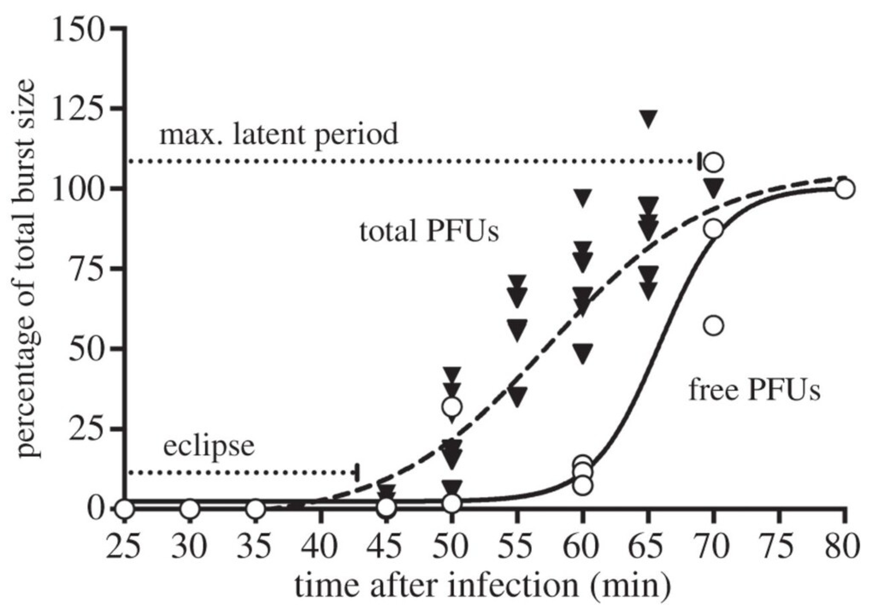
Figure 2.
Annotated one-step growth curve. The curve is based on the data of Adams [1], p. 476. Adams suggests ignoring spuriously high data points (“Ignore?”), as likely resulting from a cell-lysis event occurring in the course of plating (Section 3.3.6). We otherwise suggest that the Adams OSG experiment should be emulated by phage researchers first in terms of the many time points taken before, during, and after lysis – without using dogmatically consistent intervals – and then in terms of its presentation. Note that pre-lysis average and median values were both calculated, with both being identical at 101.5 (normalized in the figure to 1). Burst size varied from 109.5 to 110.3 based on averaging of the post-rise titers vs. using median. For determination of the post-rise value, note that we have ignored time points taken while titers appeared to be still rising. We thus have based this number (~11,200 used the actual Adams-presented data) on the last six rather than the last seven time points, as representing a judgement call. Note also that Adams indicates that the end of the constant period occurs between 21 and 23 minutes rather than the average value of 22 minutes that we claim in the figure.
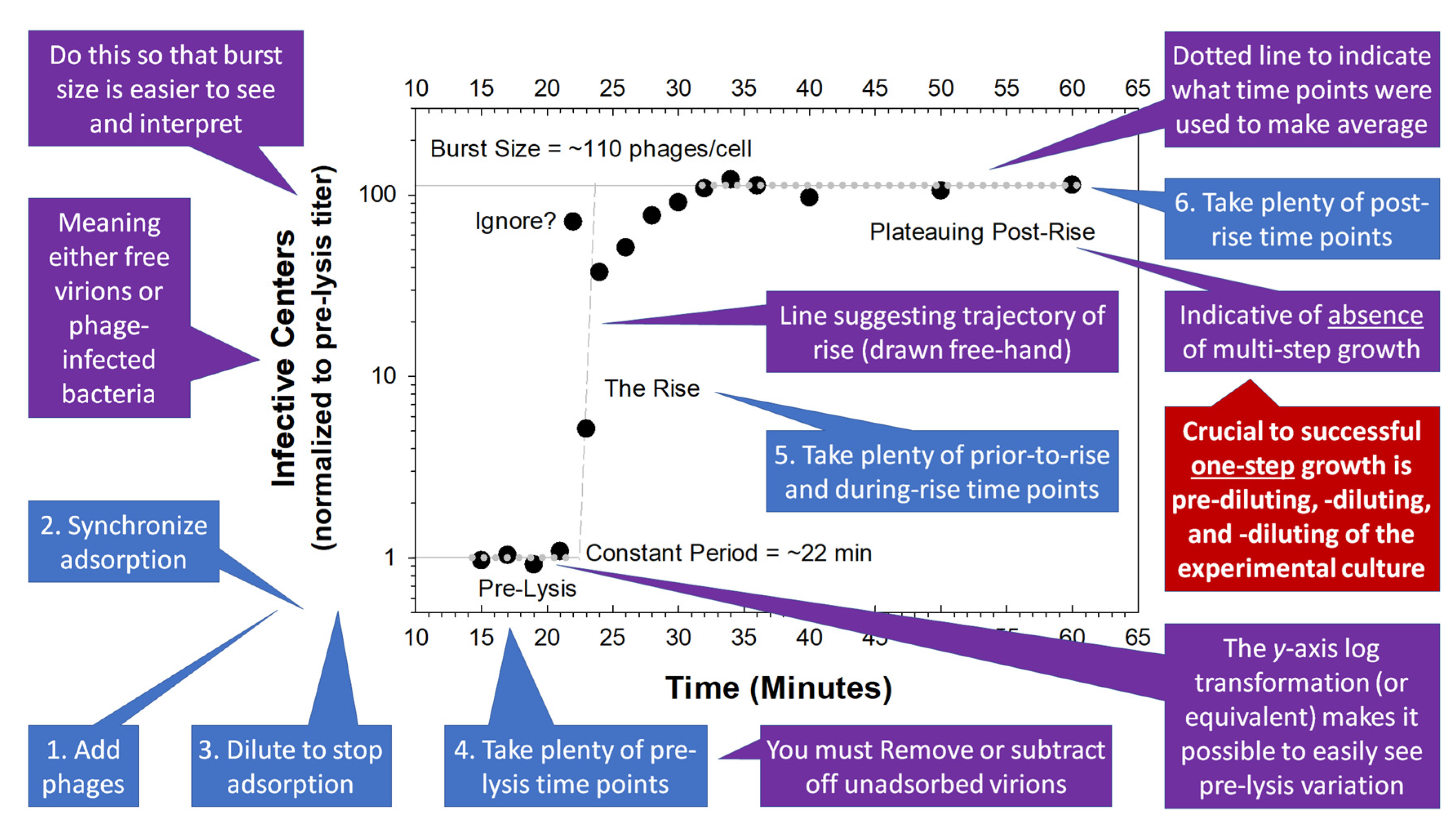
Figure 3.
Protocol for one-step growth with minimal dilution steps. This protocol is based on that of Hyman and Abdon [35], which in turn pays homage to the OSG approach presented by Adams [1]. Note that step (K) from the text is not shown. The test tube image is sourced from https://www.vectorstock.com/royalty-free-vector/comic-cartoon-science-test-tube-vector-6999912.
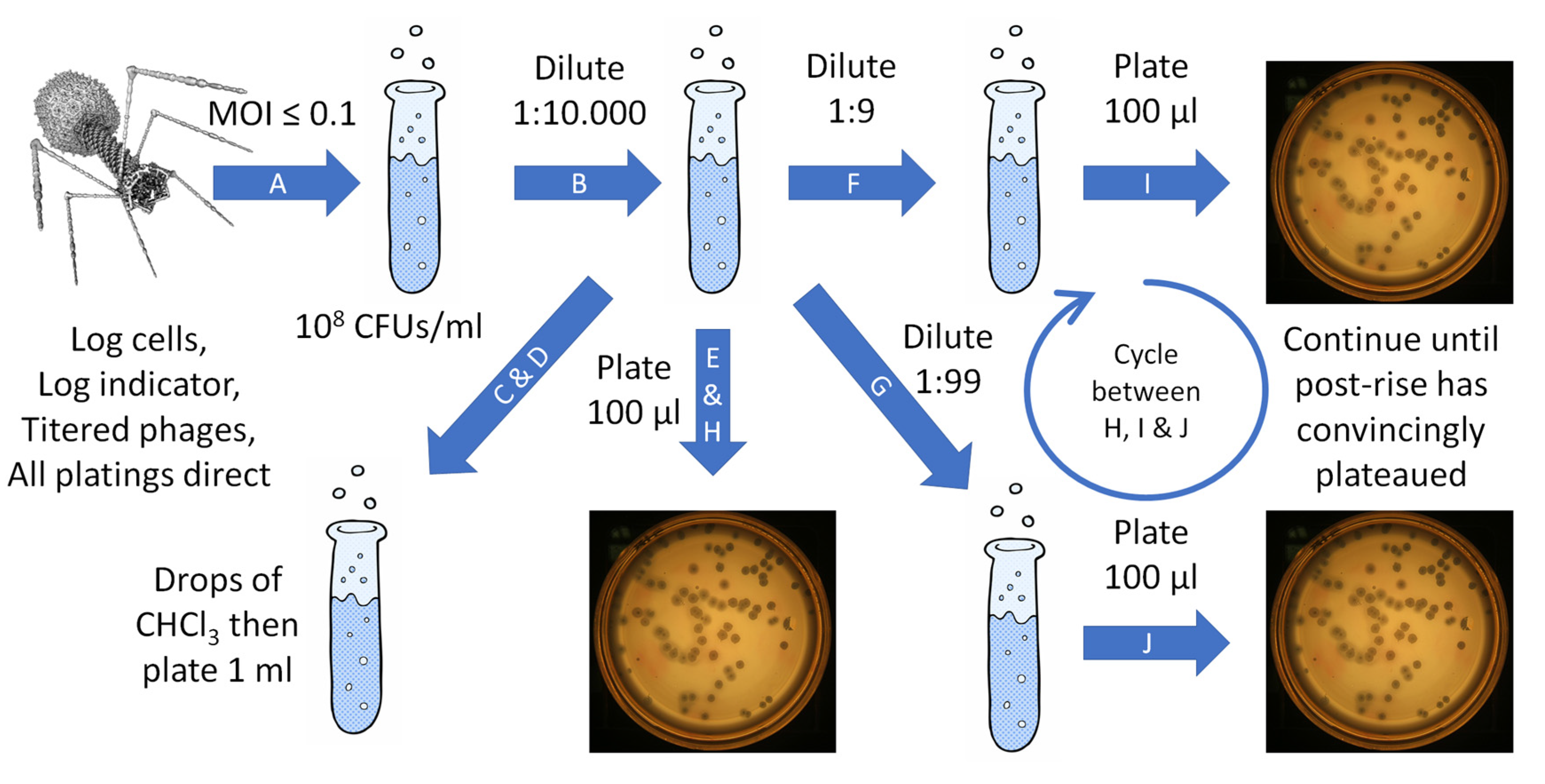

Table 1.
Definitions of key OSG terms.
| Phase, Period, or Term | Definition | Comments | Section(s) |
|---|---|---|---|
| Infective center | Either a free virion or a phage-infected bacterium that is able to form a plaque | Synonym: plaque-forming unit (PFU) | 3.3.1 |
| Adsorption | Time during which free virions are converted into bacteria-infecting phages | This should be intentionally limited in duration | 3.2 |
| Eclipse | Time during latent period prior to the intracellular formation of the first mature virion | It is not possible to define the eclipse using a standard, without artificial lysis OSG protocol | 3.3, 3.6.1, and 5.3 |
| Post-Eclipse | Time during the latent period the latent period that follows the eclipse and which ends with phage-induced bacterial lysis | We are not aware of an agreed upon name for this period; the length of this period, too, is not definable using a standard OSG protocol | 3.3, 3.6.1, and 5.3 |
| Rise | Time during which lysis across a population of phage-infected bacteria is occurring, seen as an increase in the phage titer of a culture that has a well-defined start and finish | If the rise does not have obvious end point, such that titers keep rising, then that is an indication of multi-step growth; synonyms: Burst period or burst time | 3.4 and 3.6.2 |
| Post-Rise | Time following the rise during which titers have stabilized (neither substantially rising nor falling) | If titers start to increase again post-rise, then that is an indication of multi-step growth; synonyms: Post-lysis, Plateau | 3.5 and 3.6.3 |
Disclaimer/Publisher’s Note: The statements, opinions and data contained in all publications are solely those of the individual author(s) and contributor(s) and not of MDPI and/or the editor(s). MDPI and/or the editor(s) disclaim responsibility for any injury to people or property resulting from any ideas, methods, instructions or products referred to in the content. |
© 2025 by the authors. Licensee MDPI, Basel, Switzerland. This article is an open access article distributed under the terms and conditions of the Creative Commons Attribution (CC BY) license (http://creativecommons.org/licenses/by/4.0/).
Copyright: This open access article is published under a Creative Commons CC BY 4.0 license, which permit the free download, distribution, and reuse, provided that the author and preprint are cited in any reuse.


