Submitted:
29 July 2025
Posted:
30 July 2025
You are already at the latest version
Abstract
This study presents a quantum electrodynamics (QED) framework that explains 1 the anomalous behavior of liquid water. The theory posits that water consists of two 2 coexisting phases: a coherent phase, in which molecules form phase-locked coherence 3 domains (CDs), and an incoherent phase that behaves like a dense van der Waals fluid. By 4 solving polynomial-type equations, we derive key thermodynamic properties, including the 5 minima in the isobaric heat capacity per particle (IHCP) and the isothermal compressibility, 6 as well as the divergent behavior observed near 228K. The theory also accounts for water’s 7 high static dielectric constant. These results emerge from first-principles QED, integrating 8 quantum coherence with macroscopic thermodynamics. The framework offers a unified 9 explanation for water’s anomalies and has implications for biological systems, materials 10 science, and fundamental physics. Future work will extend the theory to include phase 11 transitions, solute interactions, and the freezing process.
Keywords:
liquid water thermodynamics
; coherent domains (CDs)
; quantum electrodynamics (QED)
; two-phase model of water
; energy gap in coherent water
; isobaric heat capacity anomalies
; isothermal compressibility of water
; static dielectric constant of liquid water
; spontaneous symmetry breaking in water
; coherent–incoherent phase equilibrium
1. Introduction
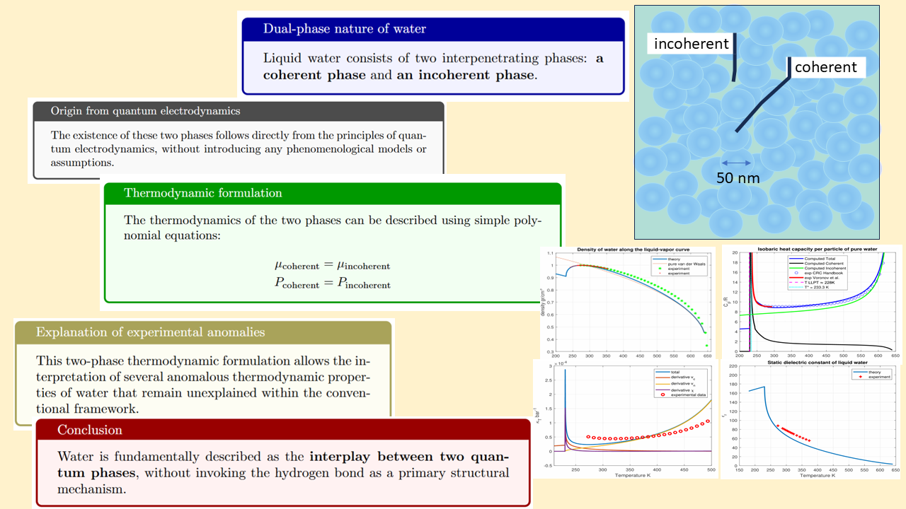
The enigmatic behavior of liquid water, illustrated by phenomena such as its maximum density, maximum isothermal compressibility, very high thermal capacity, and ultra-high dielectric constant, has fueled scientific inquiry for more than a century. These are just a few of many thermodynamic properties in which water deviates significantly from the behavior of simple liquids. In 1892, Roengten first speculated that water comprises interpenetrating "ice-like" and "fluid" structures, a classical mixture model that laid the groundwork for later two-phase theories [1]. A radical departure emerged in the 1980s with the quantum electrodynamic (QED) framework by Del Giudice and Preparata, who proposed that water sustains macroscopic coherence through photon-exchange interactions, forming ordered "coherent domains" (CDs) alongside disordered bulk regions [2,3].
Parallel developments in classical physics gained momentum with the evidence of metastable coexistence of low-density liquids (LDL) and high-density liquids (HDL) in supercooled water [4]. This was corroborated by Mishima et al. through pressure-induced amorphous ice transitions [5], while Wernet et al. used X-ray spectroscopy to identify structural motifs similar to LDL and HDL in ambient water [6].
In fact, different experimental techniques such as small-angle X-ray scattering (SAXS) and Kerr effect in liquid water show the existence of two different fluids normally interpreted as hydrogen-bond networks and individual modes governed by collisional processes [7,8].
In 2012 Del Giudice et al. refined the calculations showing that water molecules can undergo phase transitions to a coherent condensed phase, oscillating in unison with a self-trapped electromagnetic field. Such configurations imply the existence of quasi-free electrons capable of explaining a large number of biological phenomena [9].
Modern studies highlight both numerically and experimentally that thermodynamic anomalies are signatures of the existence of two separate intertwined phases [10].
In this paper, we follow the lines initially delineated by Preparata and Del Giudice [3,11] by developing the thermodynamics of the coherent and incoherent phases making the assumption that the incoherent phase behaves essentially as a polar van der Waals (vdW) fluid. Part I will provide a detailed exposition of the theory, while Part II will explore the thermodynamic properties of liquid water as derived from it. This approach will lead us to explain the origin of thermal anomalies such as density and thermal expansion (Sec. 3.3), isobaric heat capacity per particle(IHCP) (Sec. 3.4), isothermal compressibility (Sec. 3.5).
2. Part I
2.1. Physics of the Two Fluids
It is universally accepted that the most accurate description of phenomena in condensed matter lies in the realm of quantum electrodynamics (QED). Water is no exception. However, due to the enormous difficulty of the mathematical task, the solution of the equations of water physics is often approximated using semiclassical or classical models, in which the interactions between molecules are described via phenomenological potentials. The solution of the resulting classical many-body equations of motion is left to the numerical calculations of powerful computers. The thermodynamic variables are calculated by averaging the dynamic configurations over a large number of particles.
This approach, although very popular, has significant limitations due to the limited power of the available computers such as the low number of water molecules that can be simulated and the very short evolution times of the dynamic equations that can be reached. Perhaps more importantly, the potentials that are used to describe the interactions among molecules arise from phenomenological arguments rather than from first principles.
Here we approach the two-fluid picture of liquid water having its origins into the existence of a spontaneous symmetry breaking mechanism of the electromagnetic field in interaction with the water molecules. This approach was first proposed in the late 1980s by a group of Italian theoretical physicists who used high-energy physics methods to the condensed matter. The results that emerged were surprising in many ways but did not meet with the favor of the community of physicists historically engaged in the study of water, both because of the natural distrust towards colleagues from another sector and because of the methodology based on analytical calculation rather than on molecular dynamics simulations that were increasingly gaining ground in those years.
Recent advances in quantum electrodynamics (QED) have revealed that coherent domains (CDs) emerge through spontaneous symmetry breaking of the electromagnetic field in interaction with water molecules. This results in a macroscopic quantum ground state distinct from individual molecular states, as demonstrated in [9,11,12,13]. Experimental validation comes from [14], showing that vibrational spectra reveal that liquid water can be described as a mixture of high-density and low-density fractions. In Ref. [15], it is argued that the existence of a low-density, low-entropy phase in bulk water organized in tiny patches is necessary to explain the experimental observations.
After many decades, the two-fluid structure of water, initially strongly contested, is now accepted by most scientists even if the justification given is largely phenomenological. By recovering the QED approach, we obtain an analytical and accurate description of the structural, dynamic and thermodynamic properties of water that allows not only to explain the still unexplained experimental results but also to face the deep implications for biological systems, material science, and fundamental physics.
In the following are the main outcomes of the QED theory of water.
- 1)
- Liquid water is composed by two different mixed fractions over the whole range of existence of the liquid: a coherent phase where molecules are phase-locked over an extended space-time region and a incoherent (or normal) phase made up of individual molecules forming a dense incoherent fluid. The two phases are interspersed and cannot be separated as in the case of the two-fluids model of superfluid 4He. As a general rule, the incoherent phase predominates at high temperatures and gradually decreases in favor of the coherent phase with decreasing temperature in a way that will be described in the following paragraphs.
- 2)
- The coherent phase is made up by an ensemble of Coherence Domains (CDs) that can be assumed as spheres whose radius depends on the temperature. The centers of the CDs are arranged in a regular configuration in order to minimize the energy of the system. When the temperature decreases, the CDs tend to increase their size until they merge into a single macroscopic domain for sufficiently low temperature. This may account for increased viscosity when temperature is decreased and may account for the glassy nature of supercooled water [16].
- 3)
- The molecules belonging to the coherent phase are energetically separated from the non-coherent phase by an energy gap, protecting them from the thermal fluctuations. The reason of the existence of an energy gap is due to a collective ground state different from the ‘perturbative’ ground state of the isolated molecules [11].
- 4)
-
The single CD at zero temperature is characterized by a collective interaction among the water molecules through a macroscopic coherent electromagnetic field. These molecules are kept in phase by the electromagnetic field whose profile is given by [11]where , r is the radial distance from the center of the CD and 38 nm is the CD radius. The profile of the energy gap per particle for a single CD is given by , since the energy per particle is proportional to the square of the amplitude of the coherent electromagnetic field.In the bulk liquid composed by CDs, the profile of the energy gap at position is given bywhereand where are the positions of the CD centers.
- 5)
-
The CDs are arranged in a HPC configuration in order to minimize the total energy. As the temperature increases, the molecules belonging to the coherent state migrate towards the incoherent state, thus reducing the coherent fraction. A fluid of incoherent molecules is then formed which fills the interstices between the CDs and the size of the CDs gets reduced. It is worth noting that the arrangement of the CDs does not form a rigid crystal, as each CD can slide over the adjacent ones, separated by the incoherent fluid.
- 6)
- At a fixed temperature T and pressure P the total number of molecules N can be written as , being the number of molecules in the coherent phase, the number of molecules in the incoherent phase and the number of molecules in the vapor phase.
- 7)
- The molecules belonging to the coherent phase are in an excited electronic state given by the superposition of the ground state and the 5d state corresponding to an energy of 12.06 eV according to the formulawith [11], whose energy gap is =-0.3 eV per molecule. Since the excited state is spatially quite more extended than the ground state , the intermolecular distance is larger than would be predicted from the standard molecular size. Furthermore, the new electronic configuration accounts for the tetrahedral coordination of the water molecules in the coherent phase. In Ref. [17] this problem has been thoroughly discussed. This fact implies that the water molecules in the coherent phase are arranged in an ice-like spatial configuration.
- 8)
- It is worth noting that the coherence involves the electronic levels and the only, so that the nuclei of the molecules are still able to perform vibrations but not rotations limited to small angles around the equilibrium directions defined by the H-bonds that, in this context, are determined by the modified electronic distribution of the coherent water molecules [17]. The kinetic contribution to the partition function of the coherent phase is therefore purely vibrational.
- 9)
-
The incoherent phase is treated as a polar fluid, where interactions are governed by a combination of the Lennard-Jones potential and dipole-dipole forces. It remains in thermodynamic equilibrium with the coherent phase, with which it continuously exchanges particles. A rigorous approach to describing the many-body interactions within the incoherent phase would involve applying the Bogoliubov diagonalization procedure, leading to a gas of quasi-particles and a phonon/roton-like interpretation. This approach would provide a detailed understanding of the thermodynamic properties of the incoherent phase, as well as the propagation of sound in liquid water.However, in this study, we approximate the incoherent phase as a vdW liquid, whose thermodynamic properties are well established. Although this approximation does not fully capture certain characteristics of liquid water, particularly the pressure-temperature coexistence curve, our primary goal is to demonstrate the qualitative explanatory power of our theoretical framework.
- 10)
- Solidification of liquid water (freezing) will not be taken into account in the present paper since it is related to the onset of a different type of electromagnetic symmetry breaking, leading to an energy gap of a different nature. The formation of ice will be the subject of a future work.
2.2. Definition of the Coherent Spatial Profile
The spatial modulation of the amplitude of both the matter field and the electromagnetic field within a single coherence domain is approximately described by the radial profile of the spherical Bessel function of the first kind, . As shown in Reference [11] and mentioned in Section 2.1, the profile of a single coherence domain is given by Eq.(1) that decays exponentially in the peripheral regions of the domain.
During the liquid condensation phase, a large number of coherence domains are rapidly packed together, seeking maximum density due to a phenomenon of reinforcement of the evanescent electromagnetic field that connects adjacent domains, thereby providing an additional energetic gain in the gap. The result is a high-density packing of coherence domains immersed in the incoherent phase of the liquid. A simple one-dimensional calculation [3] for two neighboring CDs shows that the presence of a second CD modifies the profile to become
The packing of coherence domains ensures that the electromagnetic field profile becomes the sum of the electromagnetic fields of the various domains. The presence of many packed domains causes the isolated domain’s spherical symmetry to be lost. Therefore, we use the volumetric fraction rather than the reduced radius to characterize the coherent phase:
where is the volume occupied by the coherent phase and is the total volume occupied by the liquid.
Figure 3 illustrates the profile of the coherent electromagnetic field as a function of the coherent fractional volume for an isolated single domain and for adjacent domains.
It is difficult to determine precisely the shape of the energy profile but it is reasonably expected that the correct profile of the electromagnetic field will be found somewhere between the two extremes defined in Eqs. (1) and (5). Thus, we define in Eq. (7) a spatial profile of the domain as a linear superposition of the two extreme profiles, with the overlap coefficient kept as a free parameter.
In this manner, the function is defined as a function of the coherent fractional volume. The variation of the coherent gap as a function of the fractional volume is given by the square of the function multiplied by the value of the gap at the center of the coherence domain, according to
2.3. Free Energy of the Coherent Fluid
We now need to determine the thermodynamic potentials of the coherent and incoherent phases in order to obtain the relation between the thermodynamic variables P and T and the coherent phase.
The free energy per particle of the coherent phase can be expressed as:
where . The reference density corresponds to the density at which the Lennard-Jones potential reaches its minimum energy in the coherent phase and is treated as a free parameter in the following.
The coherent state, as a singular collective quantum state, is inherently defined at absolute zero temperature. This arises from the fundamental observation that, since the quantum phases of the electronic wavefunctions of individual molecules are locked to a common value, they cannot exhibit an arbitrary phase factor of the form , which is characteristic of an ensemble of incoherent particles following a Boltzmann statistical distribution. As a result, the positional energy of the water molecules is independent of temperature.
This argument does not extend to the vibrational degrees of freedom of the water molecules, which exhibit normal thermodynamic behavior, as described below.
To characterize the short-range electrostatic interaction within the coherent phase, we utilize a Lennard-Jones potential. At absolute zero temperature, the single-particle free energy associated with this potential depends only on the density and is given by
where is taken as a free parameter (see Section 3.2). Note that and differ from those in the incoherent phase because the molecules in the coherent phase occupy an excited electronic state. As a result, they are larger than their incoherent counterparts, which in turn alters both the depth and equilibrium position of the Lennard-Jones potential (Figure 4). The values of and have been determined through numerical fitting of experimental data.
The free energy contribution due to the energy gap is given by:
where b=0.84 has been determined by a fit of the calculated energy gap as a function of density by solving numerically the equations in Refs. [11,13].
Due to the strong electrostatic forces generated by the coherent electronic configuration, the rotational motion of the molecules is almost entirely suppressed, reducing them to minor librations around their equilibrium positions.
Although the dipole-dipole positional energy could, in principle, be calculated numerically, in this analysis, we approximate it with a constant value, treated as a free parameter:
The vibrational dynamics of coherent water molecules, represented by , is associated with the vibrations of the oxygen and hydrogen nuclei around their equilibrium positions and is restricted by the electrostatic cage imposed by the coherent electronic state. Each water molecule has 6 degrees of freedom, namely the librational motions around the three spatial axes, the two vibrational modes, asymmetric and symmetric stretching and the bending.
We will approximate their dynamics to the dynamics of one-dimensional harmonic oscillators so that their free energy can be written as:
where represents the density of states that are normalized so as to fulfill the normalization condition:
The total number of degrees of freedom is six, consisting of three degrees of freedom associated with the librational motions around the three spatial axes, along with the two vibrational modes, asymmetric and symmetric stretching and bending.
The contributions from the asymmetric stretching, symmetric stretching, and bending modes, for which , are essentially independent of temperature. As a result, Eq. (13) can be approximated by:
The free energy contribution from the higher-frequency modes thus becomes a temperature-independent constant, which can be incorporated into the additive fitting parameter .
Although the total number of vibrational modes per molecule must be six, the actual distribution of the vibrational density of states in liquid water is not known with certainty. Only the low-energy modes (with meV) are thermodynamically relevant at room temperature, due to the Boltzmann population factor. The assumed form of used in this work is reported in Table 1, where we have approximated the spectral density of states as the sum of two delta functions, weighted with . These values play a key role in the determination of the isobaric heat capacity (see Section 3.4).
Finally, the relationship between pressure and density is given by:
where . Note that is not uniform inside the coherent phase since the energy gap depends on the volumetric fraction . Therefore, we need to compute pressure and density of the coherent phase as a function of . We perform such a calculation in Section 2.5.
2.4. Free Energy of the Incoherent Fluid
A more accurate description of the dynamics of the incoherent fraction would, in principle, require a Bogoliubov diagonalization of the matter field fluctuations around the coherent background configurations. In the present work, however, we adopt a simplified approach by modeling the incoherent phase as a van der Waals fluid. We are aware that this approximation is quite crude in certain respects—most notably in its description of the pressure–temperature liquid–vapor coexistence curve.
For the incoherent phase at equilibrium with the vapor, the free energy per particle is given by
where
is the van der Waals contribution to the free energy [18], with a and b being the standard van der Waals parameters. These are related to the critical temperature and critical pressure by
The term represents the contribution due to dipole-dipole interactions. Liquid water is highly polar, being the dipole moment of vapor water molecule D [19], which is equivalent to eV−1, and the strength of the interaction is controlled by the Debye-Langevin parameter which in the whole thermal range of existence of the liquid is larger than 1, implying that the average energy of adjacent dipoles is always larger than the average kinetic energy of the molecules . This observation suggests that the behavior of dipoles is inclined towards organizing themselves into quasi-crystalline formations, which results in the disruption of rotational symmetry. A basic computation of free energy by averaging over the orientations of dipoles does not furnish an accurate estimate of the free energy in this case. To achieve a more dependable assessment of this quantity, one might consider employing a numerical approach. This can be effectively achieved using computational techniques in molecular dynamics, which provide more precise insights into the system’s free energy profile.
The generalized assertion that can be made is that, due to lack of the rotational symmetry, the free energy is linearly proportional to rather than being proportional to , which is the case in the regime where is small. Consequently, we assume that the dipole-dipole free energy is proportional to the reduced density :
However, this term should not be included in the free energy calculation to avoid double-counting its effects. The impact of this interaction is already reflected in the experimental values of the critical temperature and critical pressure . The key point is that including this term does not change the form of the free energy but only adjusts the value of the van der Waals coefficient a by , which is already accounted for in the experimental data for and . Therefore, we set eV.
Finally, the term accounts for the residual dynamics of hindered rotations—molecular librations around equilibrium orientations—as well as for the vibrations of the hydrogen atoms, similarly to what was considered for the coherent phase.
As in the coherent case, we assume a total of six vibrational degrees of freedom: three associated with bending, asymmetric stretching, and symmetric stretching, and three corresponding to librational modes. However, as in the coherent phase, only the librational (low-energy) modes contribute significantly to the thermodynamics, since the higher-frequency modes remain essentially unexcited in the temperature range relevant for liquid water.
Although some difference in the vibrational density of states between the coherent and incoherent phases is expected especially in the stretching modes [12], in the present work we approximate the function to be the same in both cases.
The vibrational free energy can therefore be written as
where C is an unimportant constant that will be absorbed in the parameter .
2.5. Solution of the Equilibrium Equations and Calculation of the Coherent Fraction
The analysis of liquid water reveals a two-phase composition: an incoherent phase behaving as a polar vdW fluid, and a coherent phase consisting of coherence domains (CDs) of polar molecules at essentially zero translational temperature (though vibrational components remain incoherent). These phases coexist with the vapor phase along the liquid-vapor coexistence curve in the plane. The thermodynamics of this system involves determining the densities of all three phases and their equilibrium pressure.
While the vapor and incoherent phase pressures and densities are known from vdW solutions, the coherent domain’s internal density and pressure require careful analysis due to spatial potential gradients.
For convenience we will isolate the positional component of the coherent free energy by defining the component independent of temperature as:
At thermodynamic equilibrium, the chemical potentials of the coherent and incoherent phases must be equal at the CD boundary. The coherent chemical potential is given by:
where the tilde superscript means division by the reference density , and is given by:
The solution requires solving the coupled equations for pressure equality and chemical potential equality at the CD boundary, namely
where and .
Eqs. (26) determine both the coherent fraction and the density profile within the CDs as a function of temperature along the liquid-vapor coexistence curve.
To solve for the equilibrium conditions, we can isolate from both the chemical potential and pressure equations (24) and (25). Eq. (26a) can be reformulated as
Similarly, from the pressure equality (26b) at the boundary:
The physical solution must satisfy both equations simultaneously, which means finding values of where . This can be visualized by plotting both expressions as functions of for different temperatures as shown in Figure 5.
The intersection points provide both the equilibrium density at the CD boundary (, from the x-coordinate) and the corresponding value of (from the y-coordinate) at each temperature. The value of must be between 0 and 1 for physical solutions. When , the coherent fraction is 0, and when , the coherent fraction is 1.
The numerical solutions of Eqs. (26) are shown in Figure 6 for and in Figure 7 for the density (blue curve). Figure 8 and Figure 9 show the profile of reduced coherent density and pressure inside the coherent phase as a function of the inner reduced volume.
The average density within the CD can be calculated by integrating over the volume:
and the result is shown in Figure 7 (orange curve).
Finally, the molar coherent fraction, shown in Figure 6, is determined by:
where is the density of the normal (incoherent) phase.
3. Part II
3.1. Thermodynamic Properties
In this section, we present the thermodynamic properties of liquid water derived from the theoretical framework developed in this work. Although not all the calculated quantities accurately reproduce the experimental data, the main focus lies in the theory’s ability to capture the general trends and qualitative behaviors of these properties as a function of thermodynamic parameters such as pressure and temperature. The simplicity and effectiveness of the present theory in capturing the overall trends of liquid water’s thermodynamic behavior, despite some quantitative discrepancies primarily arising from the limitations of the vdW model, underscore its utility in providing fundamental insights into the complex nature of water. By bridging quantum coherence with classical thermodynamics, the framework offers a robust foundation for understanding water’s anomalies, paving the way for future refinements and applications.
The following calculations illustrate the predictive capacity of our theory and its relevance in understanding the general thermodynamic landscape of water under varying conditions.
3.2. Parameter Optimization
The theory depends on a number of parameters whose values are not known with high precision. Given this uncertainty, a parameter optimization procedure was carried out by minimizing the mean squared error between certain thermodynamic quantities predicted by the theory and the corresponding experimental values over a range of temperatures.
The objective function used in the optimization is defined as
where denotes the mean normalized squared error associated with a given thermodynamic quantity q, and is defined by
with N representing the number of experimental data points available for quantity q, and the corresponding temperatures.
The parameters selected for optimization are indicated in Table 2, together with their optimized values.
The objective function was minimized using a MATLAB routine based on the FMINCON optimization function.
3.3. Density and Thermal Expansion Coefficient
The density anomaly is probably the most puzzling behavior of water. It is at the base of life in the oceans and contributes to determine the climate on Earth. Unlike most other liquids, water exhibits a maximum density at 4 °C under ambient pressure and expands when cooled below this temperature.
In our theory, at temperature T the molecular volume of liquid water is the weighted average of the molecular volumes of the coherent and incoherent phases, the weight being the volumetric coherent fraction
The density is therefore
where . The computed density along the liquid-vapor curve of coexistence is shown in Figure 10. In Figure 11 is shown the computed isobaric thermal expansion coefficient.
The anomaly arises from the fact that, when temperature decreases, the increasing density of the incoherent phase is balanced by the decrease of its fraction, leading to the existence of a maximum of the density which happens to be at 4 °C at atmospheric pressure.
3.4. Isobaric Heat Capacity
An intriguing and yet to be elucidated characteristic of liquid water pertains to its isobaric heat capacity per particle (IHCP), which exhibits a notable minimum at a temperature of 309 K under standard atmospheric pressure and a sharp decrease in the range 228–235 K [20,21]. In our theoretical framework, the contribution to the IHCP arises from the standard incoherent component and the vibrational degrees of freedom of water molecules, supplemented by the additional contribution of the coherent molecules transitioning out of the zero-temperature state and migrating towards the incoherent phase. This latter contribution becomes particularly significant at low temperatures, where the derivative of increases sharply, and is absent in existing models of liquid water’s IHCP to date.
The enthalpy resulting from the contribution of the two phases can be written as
where
where are the entropies of the coherent and incoherent phases respectively. corresponds to the entropy of the vibrational configurations only, being the positional degrees of freedom frozen at zero temperature by their coherent nature, so that we can write .
The IHCP is given by
It is instructive to examine in detail the various terms contributing to the IHCP by expanding Eq. (35). The IHCP may be expressed as the sum of the following components:
It is interesting to note that the term is analogous to a "latent heat" of transformation from the coherent to the incoherent phase, modulated by the rate of change of the coherent phase with temperature and accounts for the sharp increase of the IHCP at low temperature.
The relationship between the chemical potential and the enthalpy per particle is given by , where denotes the entropy of the coherent and incoherent phases. Given the equality of the chemical potentials for the two phases, we derive:
Here represents the contribution from particles transitioning from the coherent to the incoherent phase, with the difference primarily arising from entropy variation.
The coherent and incoherent vibrational terms of the entropy are given by the standard expression for the harmonic oscillator
where and are taken from Table 1.
Equation (39a) depends on the absolute entropy of the incoherent phase. However, the entropy of a vdW fluid is inherently defined only up to an additive constant , since its low-temperature behavior becomes intrinsically quantum and deviates from the classical expression, which exhibits a logarithmic divergence as temperature approaches zero. To address this, we introduce a constant term into the vdW entropy expression, which will later be calibrated against experimental data.
Accordingly, Eq. (39a) is reformulated as
where the entropy is expressed in terms of the known quantities and using the relation . The constant has been introduced to account for the aforementioned uncertainty in the absolute value of the vdW entropy.
The expression in (39b) originates from the thermal capacity of the quantum oscillators with strength and oscillation frequency , as described in Table 1.
Finally, the formula in (39c) represents the contribution of the vdW and vibrational components within the incoherent phase. The explicit expression for the temperature derivative of the vdW enthalpy at constant pressure can be obtained through straightforward algebraic manipulation, leading to
The calculation of is shown in Figure 12 where we have chosen and where are detailed also the contributions of the three terms of Eqs. (39).
The computed values deviate from experimental measurements by less than 10% on average. The calculation accurately reproduces the existence of the minimum—a distinctive hallmark of liquid water’s IHCP and, more importantly, the sharp increase of in the thermal range 228-235 K. To this day, this phenomenon lacks a fully satisfactory explanation in the literature. However, we believe that our theory captures its essential nature by merely evaluating the temperature derivative of enthalpy.
3.5. Isothermal Compressibility
The isothermal compressibility of liquid water has historically been one of the puzzling properties of water [22]. The anomaly is characterized by a minimum in compressibility at 319 K, which still lacks a structural explanation.
In our approach, this anomaly finds a natural explanation, attributed to the differing behavior of the two phases. The isothermal compressibility is defined as
where v is the volume per molecule, P is the pressure, and T is the temperature.
This expression can be rewritten by considering the contribution of the two phases:
where represents the volumetric fraction of the coherent phase, and are the volumes per particle of the coherent and incoherent phases, respectively.
The derivatives with respect to pressure of , , and can all be evaluated numerically, given that their expressions are known. Specifically, depends on pressure via Eq. (28), while and are determined by the equations of state (16) and (22), respectively.
By performing the numerical differentiation at constant temperature and substituting the results into Eq. (44), we obtain the outcome depicted in Figure 13, where a minimum is clearly visible and a sharp increase at lower temperatures with a peak at K.
The computed values of the compressibility do not accurately reproduce the experimental data for , since the van der Waals model is highly inaccurate in calculating for the incoherent phase. Nonetheless, the inclusion of the coherent contribution captures both the presence of a minimum and the divergence of at the temperature of the liquid–liquid critical point (LLCP).
3.6. Static Dielectric Constant
The static dielectric constant of liquid water is notably large, and in previous models, its behavior is not easily described unless several simplifying assumptions are made. Our proposed theory, however, provides an accurate description of this constant as a function of temperature within a certain level of precision.
3.6.1. Coherent Component of the Static Dielectric Constant
In the dipole approximation, the interaction Hamiltonian describing the coupling between the external electric field and the electronic system confined within the coherence domain is given by
where denotes the electric field and e is the elementary charge.
The coherent electronic state of the system, in the absence of the external field, can be written as a linear superposition of the ground state and an excited state , namely
where the mixing angle quantifies the degree of mixing between the two states. The normalization condition for the coherent state is
ensuring that the total probability is conserved.
When the external field is present, the macroscopic polarization is defined as the expectation value of the position operator over the coherent state modified by the field. This yields
where is the number of coherent electrons, and denotes the coherent state in the presence of the external electric field.
By applying first-order time-independent perturbation theory, we obtain
where =12.06 eV is the energy of the excited state , are the energies of the various excited levels of the water molecules and =-0.29 eV is the energy of the coherent state. Substituting Eq. (49) into Eq. (48), we obtain
where
The component represents the susceptibility associated to the deformation of the ground state of the water molecule subjected to the electric field. Its value is very small due to the large energetic distance from the other excited states and has been computed to yield .
The term represents the mixed term resulting from the combination of two states to produce the coherent state. Since these states oscillate at different frequencies, the time average of this contribution vanishes.
The last term, , yields a significant contribution due to the fact that the energy denominators in the sum are small, as the excited state lies in close proximity to many unperturbed levels. However, we cannot calculate it directly due to the unknown value of . Nonetheless, we can estimate it by approximating the excited states of the single molecule as the energy levels of a harmonic oscillator.
The oscillator strength between energy levels i and j for a harmonic oscillator is defined as
and the energy levels close to , shown in Table 3, are approximately evenly spaced. Assuming that the energy levels can be approximated by those of a harmonic oscillator, we can adopt the following approximation:
Here, we approximate and have used the relation
We evaluate the sum as follows:
Finally, using , we arrive at
where we we have substituted .
Next, we proceed to determine . We restrict the range of the levels participating to the oscillation to the levels with an energy higher than 11 eV and we find = 0.21 eV.
Finally, by substitution into Eq. (56) (, , , ) we obtain . The value of the coherent fraction of the static dielectric susceptibility of liquid water has been experimentally measured at room temperature [23], yielding a value of approximately 156. In that work, a good fit to the measured data is obtained by assuming the coexistence of two fractions with distinct dielectric properties. The experimentally determined value is in satisfactory agreement with the value calculated in our theory.
3.6.2. Evaluation of the Dielectric Constant
We can now determine the static dielectric constant of liquid water as a function of temperature by weighting the contributions of the coherent and incoherent phases according to their molar fraction, :
where the incoherent contribution is described using the Debye-Langevin polarizability given by
The resulting calculation is presented in Figure 14. The theory predicts a singularity in the static dielectric constant at the same temperature where the isothermal compressibility, isobaric heat capacity per molecule, and thermal expansion coefficient exhibit singular behavior.
4. Discussion and Conclusions
To achieve a comprehensive understanding of the origin of water’s behavior, particularly the properties that make it the most vital liquid for the existence of life on Earth, we have developed a theory grounded rigorously in the first principles of quantum electrodynamics (QED). This theoretical framework enables us to address a fundamental question that has intrigued physicists in recent years: is water a homogeneous or an inhomogeneous fluid?
A compelling model proposed by Nilsson and Pettersson [22] describes water as consisting of two coexisting liquid phases, characterized by fluctuations between two structurally distinct forms: a tetrahedral, low-density liquid (LDL) and a distorted, high-density liquid (HDL). These configurations are supported by various modeling techniques. However, the mechanism by which these heterogeneous fluctuating structures could evolve into metastable phases remains an open problem.
Our theory challenges the conventional view that hydrogen bonding serves as the fundamental explanation for the behavior of liquid water. This traditional perspective relies heavily on the empirical adjustment of parameters such as bond lifetime and strength, rather than deriving them from first principles. Consequently, such models are not genuine theories but phenomenological approximations that offer only partial and descriptive insights into the nature of liquid water.
Within our QED-based framework, hydrogen bonds are understood to result from the deformation of electronic distributions in coherent molecular domains. As shown in Eq. (4), this deformation induces a directional angular dependence in the electronic charge density, naturally accounting for the tetrahedral coordination of water molecules observed in neutron and X-ray scattering experiments [6]. Furthermore, the disappearance of hydrogen bonding at elevated temperatures is consistent with our theoretical predictions: as temperature rises, the proportion of coherent molecules diminishes, leading to the weakening and eventual disappearance of hydrogen bonding.
On the mesoscopic scale, CDs exhibit a striking organizational duality. While adopting a hexagonal close-packed (HCP) arrangement (see Figure 1 and Figure 2), the system simultaneously preserves fluidity through lubricated sliding mediated by the incoherent phase. This coexistence of structural order and dynamic disorder resolves the long-standing paradox of water’s anomalous viscoelastic properties, which combine long-range electromagnetic coherence with short-range molecular mobility.
The theory introduces three foundational advances:
- It elucidates the physical mechanisms underlying the formation and stability of the distinct liquid phases. The coherent low-density liquid (LDL) phase arises via spontaneous symmetry breaking of the electromagnetic field, resulting in macroscopic quantum domains with an average size of nm characterized by an energy gap and a spatial distribution described by the spherical Bessel function . The HDL phase, described as a polar van der Waals fluid, fills the interstices between domains. Our solutions quantitatively determine the relative abundances of these phases over a range of temperatures, reinterpreting the so-called liquid–liquid phase transition (LLPT) not as a true critical phenomenon, but rather as the temperature threshold—upon cooling—at which the incoherent phase (HDL) vanishes.
- The theory offers a first-principles explanation for several of water’s most perplexing anomalies. The well-known density maximum at 277 K emerges from the competition between the volumetric expansion of LDL domains and the densification of the HDL phase. The observed minimum in the isobaric heat capacity near 309 K reflects a balance between the stabilization of the coherent phase and thermal excitation. Most notably, the model accounts for the sharp divergence in thermodynamic behavior near 228 K as a consequence of the complete disappearance of the HDL fraction.
- The theory resolves the longstanding quantum–classical duality exhibited by water. Below approximately 320 K, the system demonstrates macroscopic quantum coherence through extended networks of coherence domains, while simultaneously retaining classical fluidity through the intervening HDL phase. As temperature increases, the coherent fraction diminishes, leading to the gradual loss of quantum coherence and explaining the crossover to purely classical behavior near the critical point.
Future work to refine the theoretical framework presented here should address several key areas. First, although the van der Waals (vdW) model provides a simple and insightful starting point, it remains a mean-field approximation. The primary objective of this study has been to establish a foundational theoretical perspective on the nature of liquid water rather than to reproduce all thermodynamic properties in exact detail. Once this conceptual basis is solidified, further refinements can be introduced to capture the full complexity of the water phenomenology. A more rigorous treatment of the incoherent phase would involve modeling it as a manifestation of quantum fluctuations in the matter field, represented by quasi-particle excitations. This approach aligns with the framework of quantum fluids, in which excitations correspond to fluctuations around the mean-field background.
Finally, significant uncertainty remains regarding the internal molecular dynamics, particularly the energetics of vibrational modes. These degrees of freedom play a critical role in determining the thermodynamic properties of water and must be accurately characterized to improve the predictive power and quantitative accuracy of the theory.
Our results demonstrate that the anomalous properties of liquid water arise from its dual character: a quantum-coherent system coexisting with quantum thermal fluctuations. This paradigm not only resolves several long-standing thermodynamic anomalies, but also opens new avenues for research, particularly in the study of biological water interfaces and the development of quantum-inspired materials. The dynamic interplay between coherence and decoherence in water may prove to be a fundamental principle underlying its unique role in both natural processes and emerging technologies.
References
- Röntgen, W.C. Ueber die Constitution des flüssigen Wassers. Annalen der Physik 1892, 281, 91–97. [Google Scholar] [CrossRef]
- Del Giudice, E.; Preparata, G.; Vitiello, G. Water as a free electric dipole laser. Physical Review Letters 1988, 61, 1085–1088. [Google Scholar] [CrossRef] [PubMed]
- Preparata, G. QED Coherence in Matter; World Scientific, 1995.
- Poole, P.H.; Sciortino, F.; Essmann, U.; Stanley, H.E. Phase behaviour of metastable water. Nature 1992, 360, 324–328. [Google Scholar] [CrossRef]
- Mishima, O.; Stanley, H.E. The relationship between liquid, supercooled and glassy water. Nature 1998, 396, 329–335. [Google Scholar] [CrossRef]
- Wernet, P.; Nordlund, D.; Bergmann, U.; Cavalleri, M.; Odelius, M.; Ogasawara, H.; Naslund, L.A.; Hirsch, T.K.; Ojamae, L.; Glatzel, P.; et al. The structure of the first coordination shell in liquid water. Science 2004, 304, 995–999. [Google Scholar] [CrossRef] [PubMed]
- Huang, C.; Wikfeldt, K.T.; Tokushima, T.; Nordlund, D.; Harada, Y.; Bergmann, U.; Niebuhr, M.; Weiss, T.M.; Horikawa, Y.; Leetmaa, M.; et al. The inhomogeneous structure of water at ambient conditions. Proceedings of the National Academy of Sciences 2009, 106, 15214–15218. [Google Scholar] [CrossRef] [PubMed]
- Taschin, A.; Bartolini, P.; Eramo, R.; Righini, R.; Torre, R. Evidence of two distinct local structures of water from ambient to supercooled conditions. Nature communications 2013, 4, 2401. [Google Scholar] [CrossRef]
- Bono, I.; Del Giudice, E.; Gamberale, L.; Henry, M. Emergence of the Coherent Structure of Liquid Water. Water 2012, 4, 510–532. [Google Scholar] [CrossRef]
- Gallo, P.; Amann-Winkel, K.; Angell, C.A.; Anisimov, M.A.; Caupin, F.; Chakravarty, C.; Lascaris, E.; Loerting, T.; Panagiotopoulos, A.Z.; Russo, J.; et al. Water: A Tale of Two Liquids. Chemical Reviews 2016, 116, 7463–7500. [Google Scholar] [CrossRef] [PubMed]
- Arani, R.; Bono, I.; del Giudice, E.; Preparata, G. QED coherence and the thermodynamics of water. International Journal of Modern Physics B 1995, 9, 1813–1841. [Google Scholar] [CrossRef]
- Ninno, A.D.; Giudice, E.D.; Gamberale, L.; Castellano, A.C. The Structure of Liquid Water Emerging from the Vibrational Spectroscopy: Interpretation with QED Theory. Water 2014, 6, 13–25. [Google Scholar]
- Del Giudice, E.; Vitiello, G. The role of the electromagnetic field in the formation of domains in the process of symmetry breaking phase transitions. Physical Review A 2006, 74, 022105. [Google Scholar] [CrossRef]
- De Ninno, A.; De Francesco, M. Water molecules ordering in strong electrolytes solutions. Chemical Physics Letters 2018, 705, 7–11. [Google Scholar] [CrossRef]
- Majolino, D.; Mallamace, F.; Migliardo, P. Spectral evidence of connected structures in liquid water: Effective Raman density of vibrational states. Physical Review E 1993, 47, 2454–2459. [Google Scholar] [CrossRef] [PubMed]
- Buzzacchi, M.; Del Giudice, E.; Preparata, G. Coherence of the Glassy State. International Journal of Modern Physics B 2002, 16, 3771–3786. [Google Scholar] [CrossRef]
- Del Giudice, E.; Galimberti, A.; Gamberale, L.; Preparata, G. Electrodynamical Coherence in Water: A Possible Origin of the Tetrahedral Coordination. Modern Physics Letters B 1995, 09, 953–961. [Google Scholar] [CrossRef]
- Johnston, D.C. Advances in Thermodynamics of the van der Waals Fluid; 2053-2571; Morgan & Claypool Publishers, 2014. [Google Scholar] [CrossRef]
- Gregory, J.K.; Clary, D.C.; Liu, X.; Brown, M.; Saykally, R.J. The water dipole moment in water clusters. Science 1997, 275, 814–817. [Google Scholar] [CrossRef] [PubMed]
- Haynes, W.M. (Ed.) CRC Handbook of Chemistry and Physics, 97th ed.; CRC Press: Boca Raton, FL, 2016. [Google Scholar]
- Voronov, V.P.; Podnek, V.E.; Anisimov, M.A. High-resolution adiabatic calorimetry of supercooled water. Journal of Physics: Conference Series 2019, 1385, 012007. [Google Scholar] [CrossRef]
- Nilsson, A.; Pettersson, L. The structural origin of anomalous properties of liquid water. Nature Communications 2015, 6, 8998. [Google Scholar] [CrossRef] [PubMed]
- De Ninno, A.; Nikollari, E.; Missori, M.; Frezza, F. Dielectric permittivity of aqueous solutions of electrolytes probed by THz time-domain and FTIR spectroscopy. Physics Letters A 2020, 384, 126865. [Google Scholar] [CrossRef]
- Jackson, J.D. Classical Electrodynamics, 3rd ed.; John Wiley & Sons: New York, 1998; See Chapters 4 and 8 for detailed discussion on dielectric polarization and the Langevin function. [Google Scholar]
Figure 1.
HPC arrangement of the CDs. Units are CD diameters
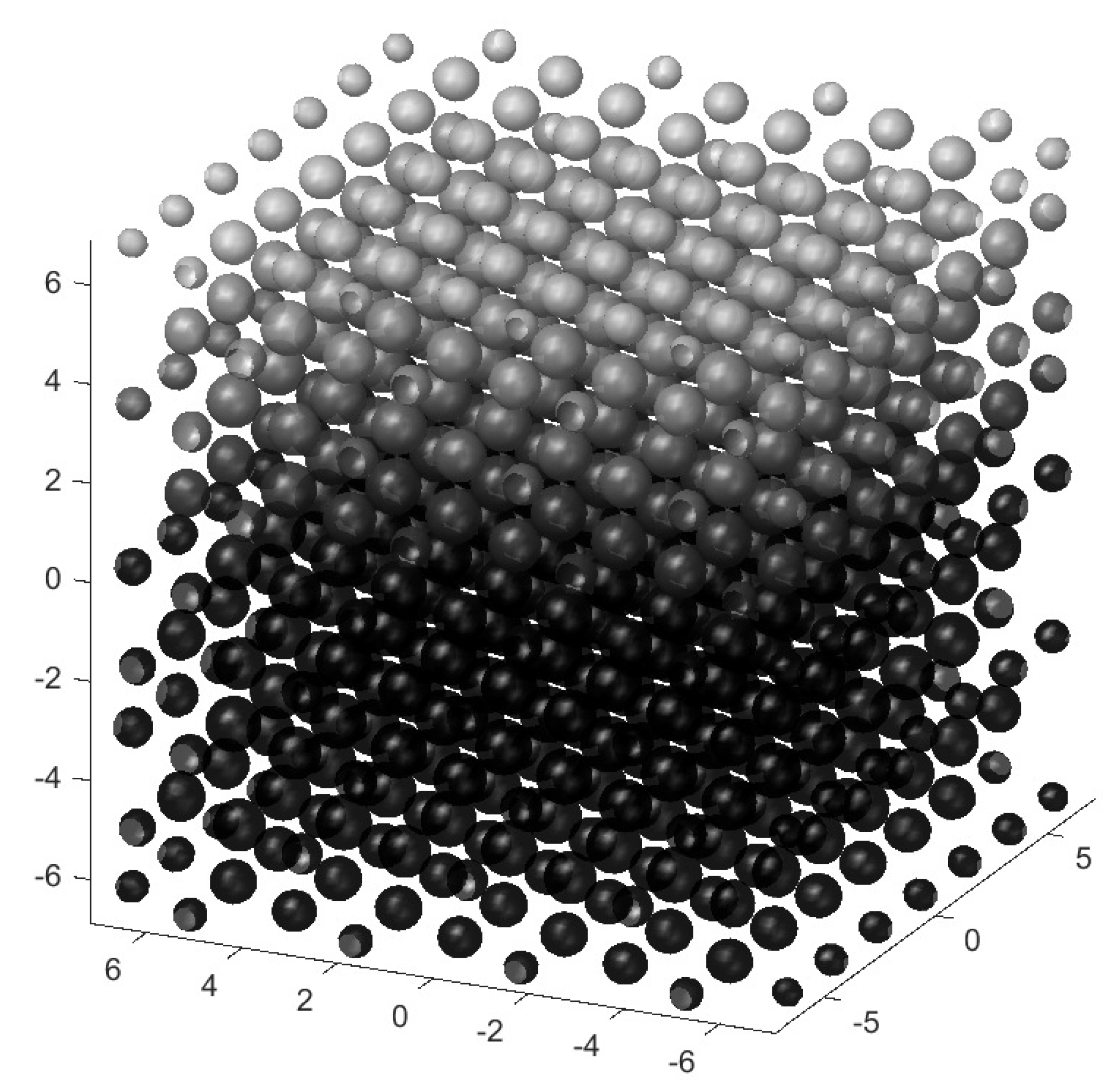
Figure 2.
Color contouring map of the profile function . Units are CD diameters
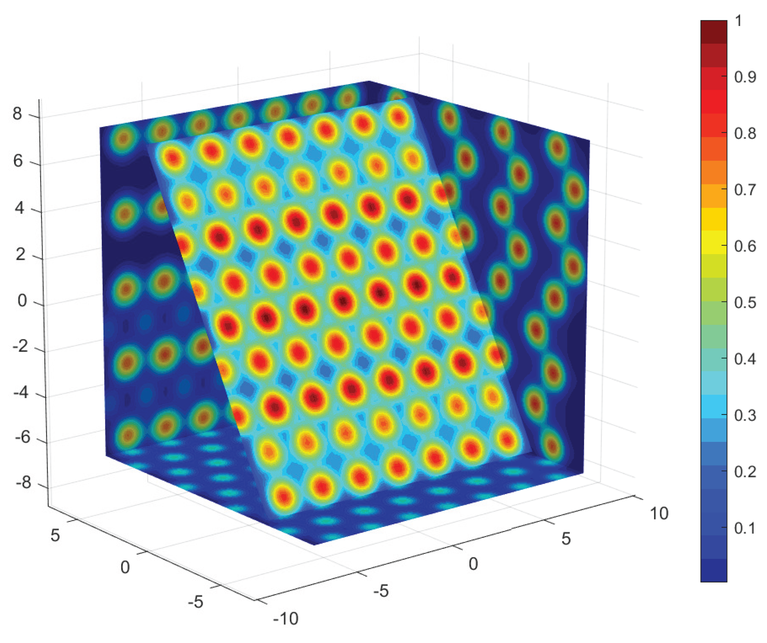
Figure 3.
Normalized profile of the energy gap as a function of the fractional coherent volume
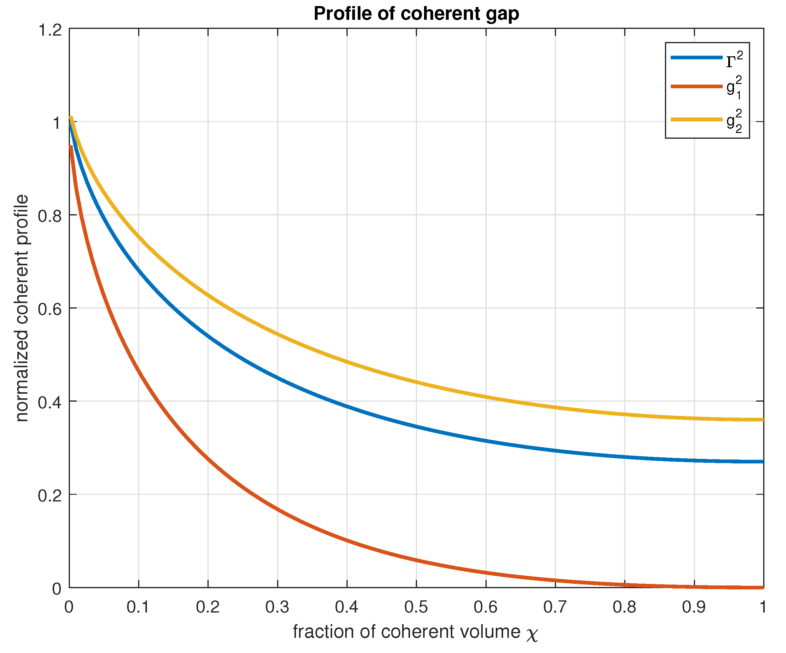
Figure 4.
Comparison of the Lennard-Jones potential for the coherent and incoherent phases.
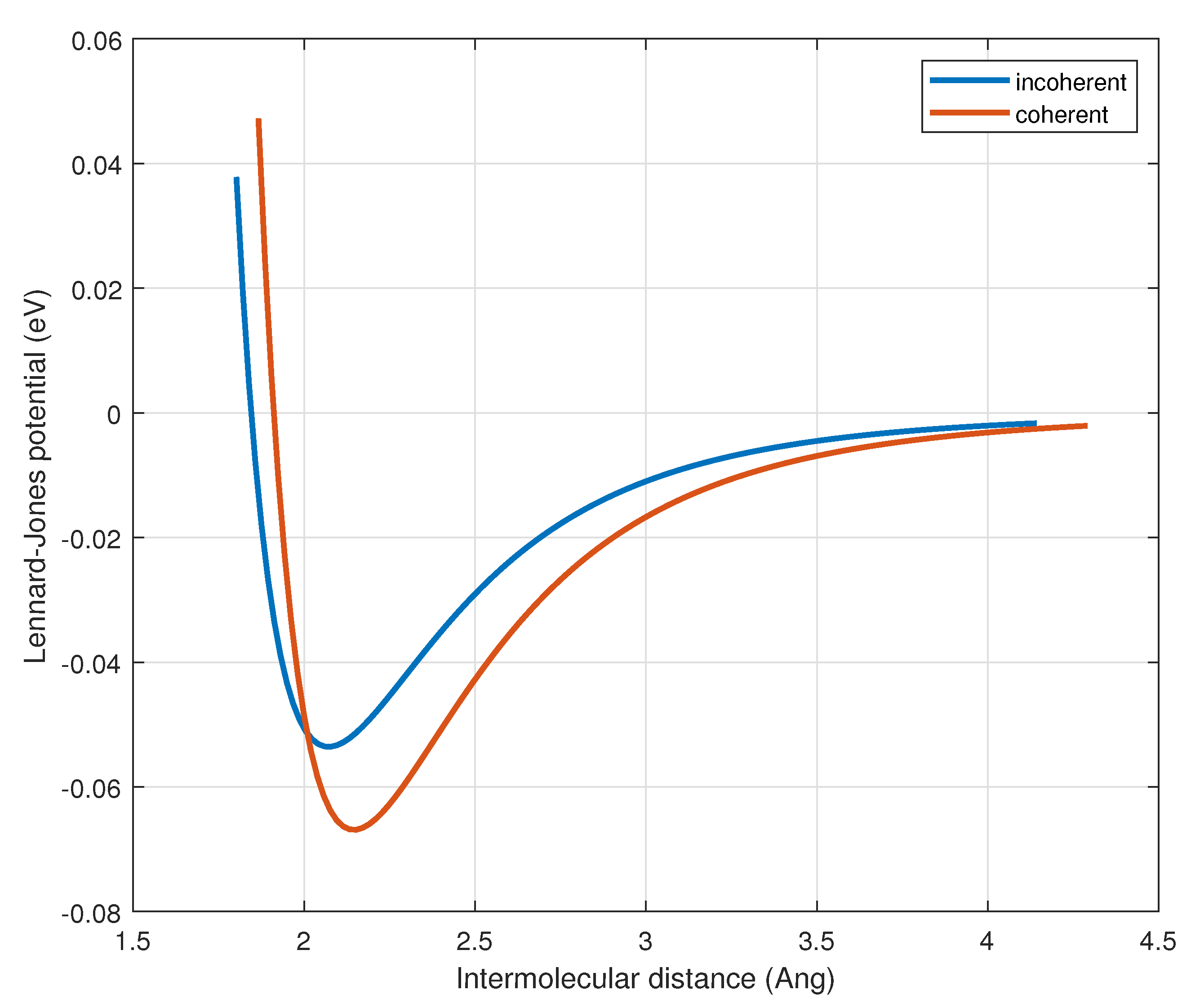
Figure 5.
Solutions for from chemical potential (solid lines) and pressure (dashed lines) equations at different temperatures. The intersections determine the physically meaningful solutions for the density at the CD boundary for in the existence interval [0 1] only.
Figure 5.
Solutions for from chemical potential (solid lines) and pressure (dashed lines) equations at different temperatures. The intersections determine the physically meaningful solutions for the density at the CD boundary for in the existence interval [0 1] only.
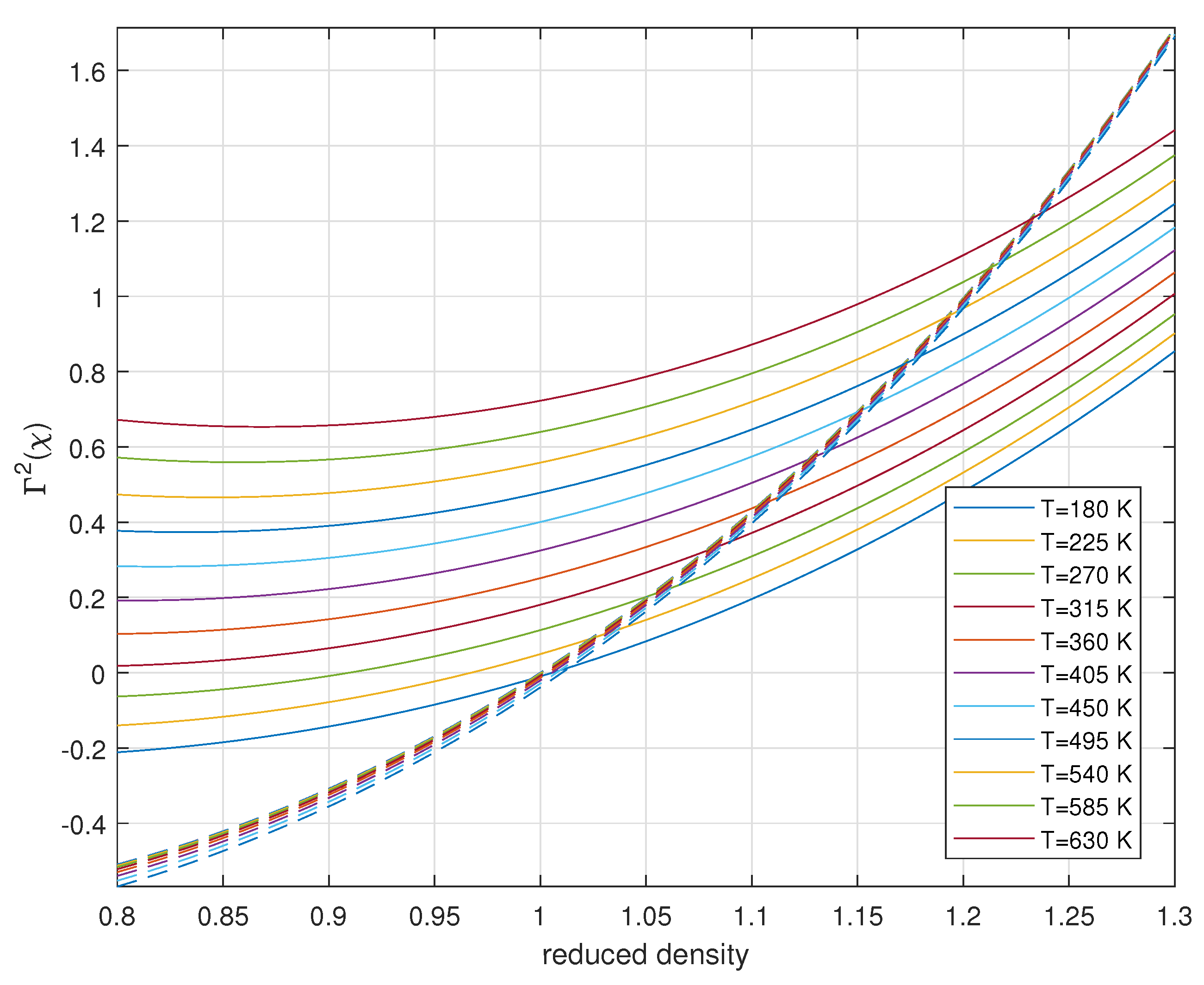
Figure 6.
Temperature dependence of both molar and volumetric () coherent fractions, showing the transition from fully coherent to fully incoherent behavior.
Figure 6.
Temperature dependence of both molar and volumetric () coherent fractions, showing the transition from fully coherent to fully incoherent behavior.
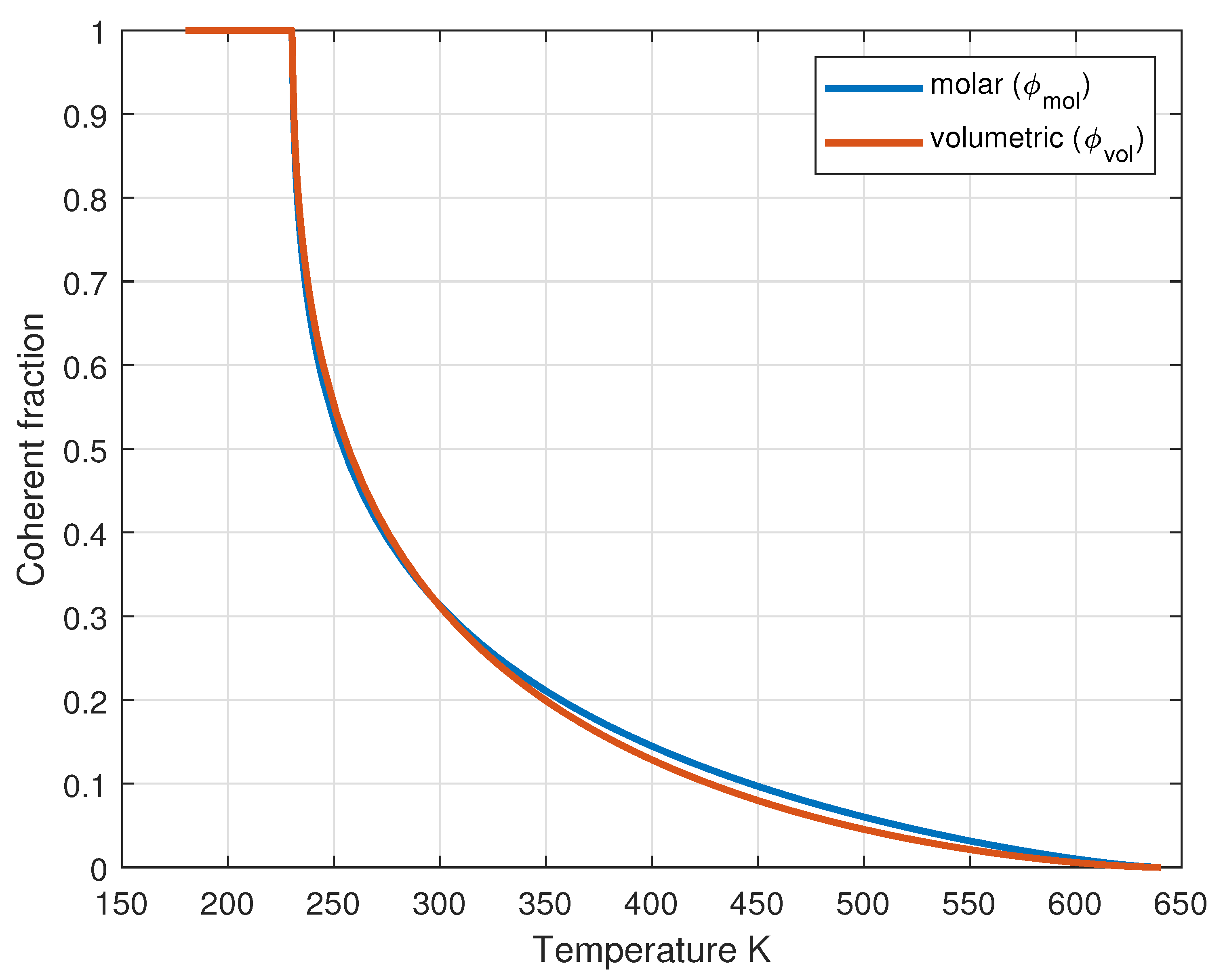
Figure 7.
Reduced coherent density at the boundary and in the bulk of the coherent phase as a function of temperature.
Figure 7.
Reduced coherent density at the boundary and in the bulk of the coherent phase as a function of temperature.
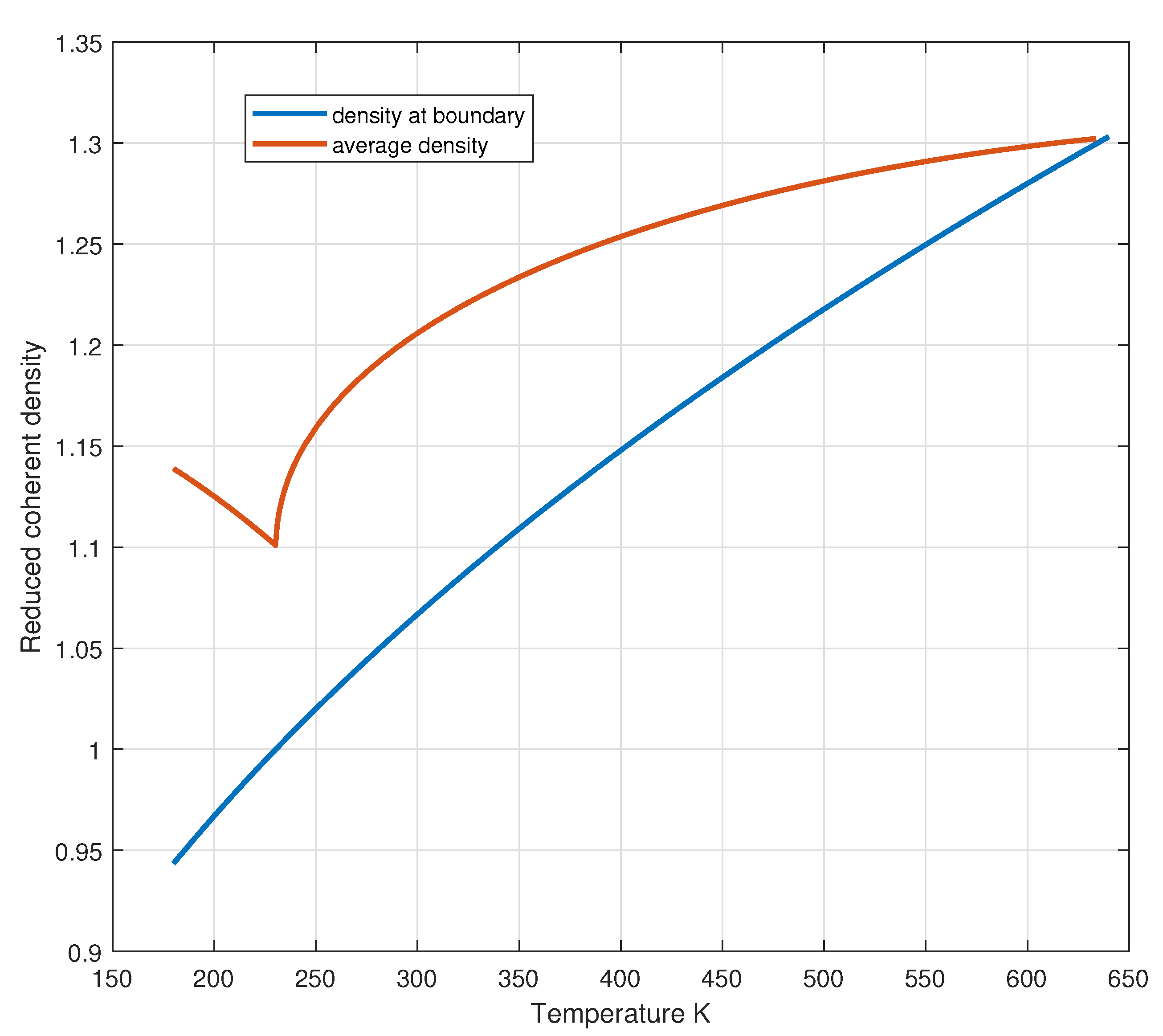
Figure 8.
Pressure profile within the coherent domain for different temperatures. The pressure increases towards the center due to the coherent potential gradient.
Figure 8.
Pressure profile within the coherent domain for different temperatures. The pressure increases towards the center due to the coherent potential gradient.
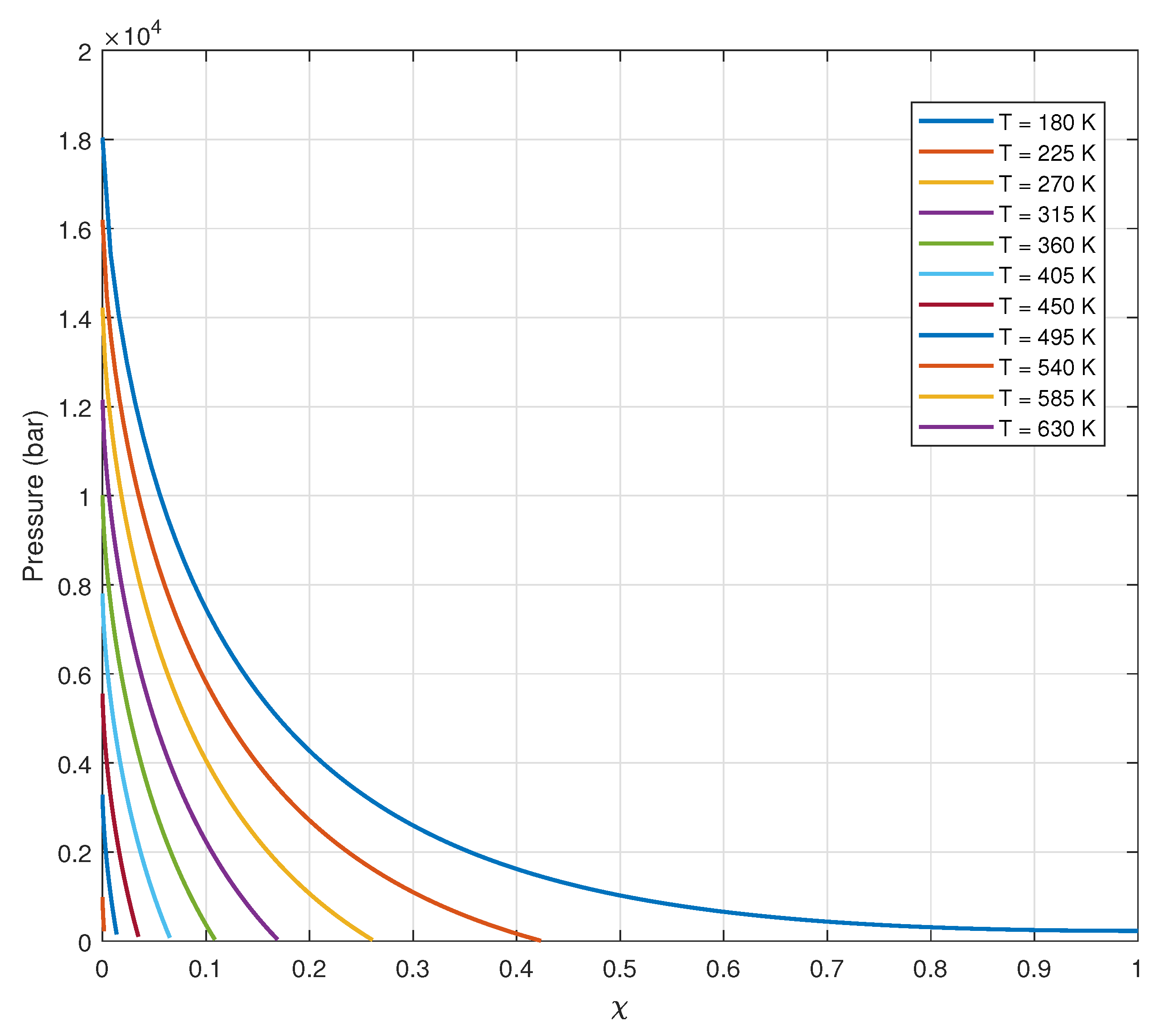
Figure 9.
Reduced density profile within the coherent domain showing increased density towards the center due to compression effects. The absence of an intersection between the density profile and the x-axis indicates that, at K, the system exhibits complete coherence .
Figure 9.
Reduced density profile within the coherent domain showing increased density towards the center due to compression effects. The absence of an intersection between the density profile and the x-axis indicates that, at K, the system exhibits complete coherence .
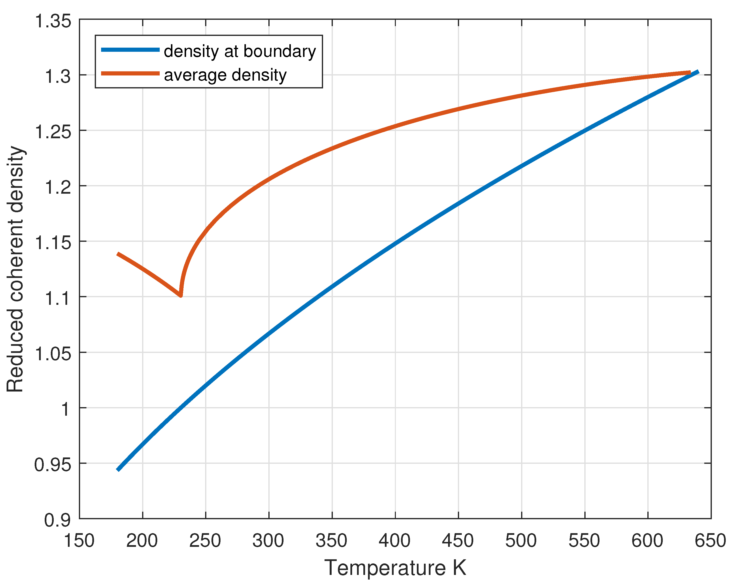
Figure 10.
Computed density of liquid water as a function of temperature along the liquid-vapor coexistence curve, compared with the experimental data [20].
Figure 10.
Computed density of liquid water as a function of temperature along the liquid-vapor coexistence curve, compared with the experimental data [20].
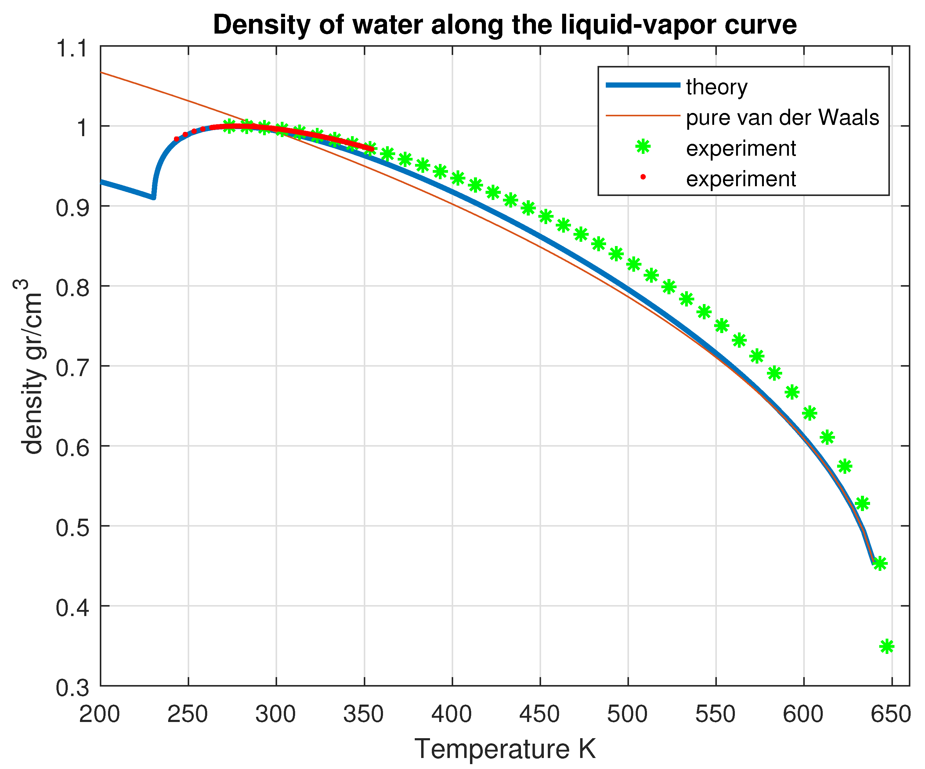
Figure 11.
Computed isobaric thermal expansion of liquid water as a function of temperature along the liquid-vapor coexistence curve compared with experimental data [20].
Figure 11.
Computed isobaric thermal expansion of liquid water as a function of temperature along the liquid-vapor coexistence curve compared with experimental data [20].
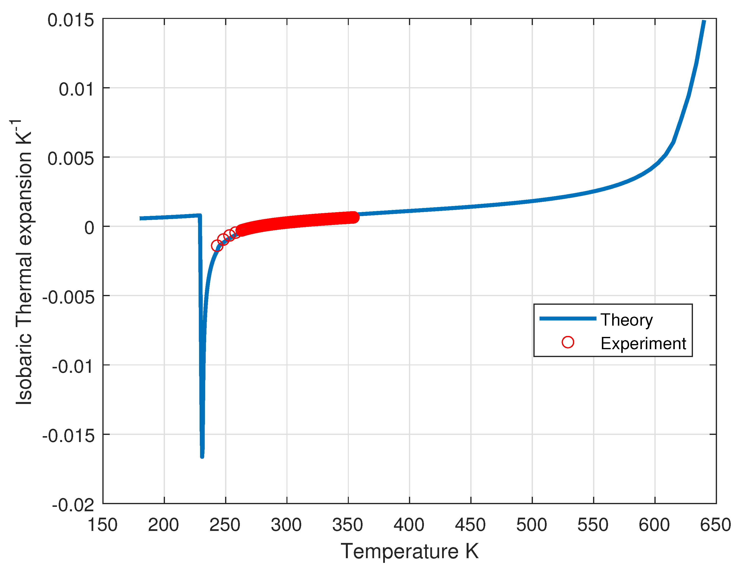
Figure 12.
Isobaric heat capacity per particle of liquid water as a function of temperature at atmospheric pressure compared with experimental data [21].
Figure 12.
Isobaric heat capacity per particle of liquid water as a function of temperature at atmospheric pressure compared with experimental data [21].
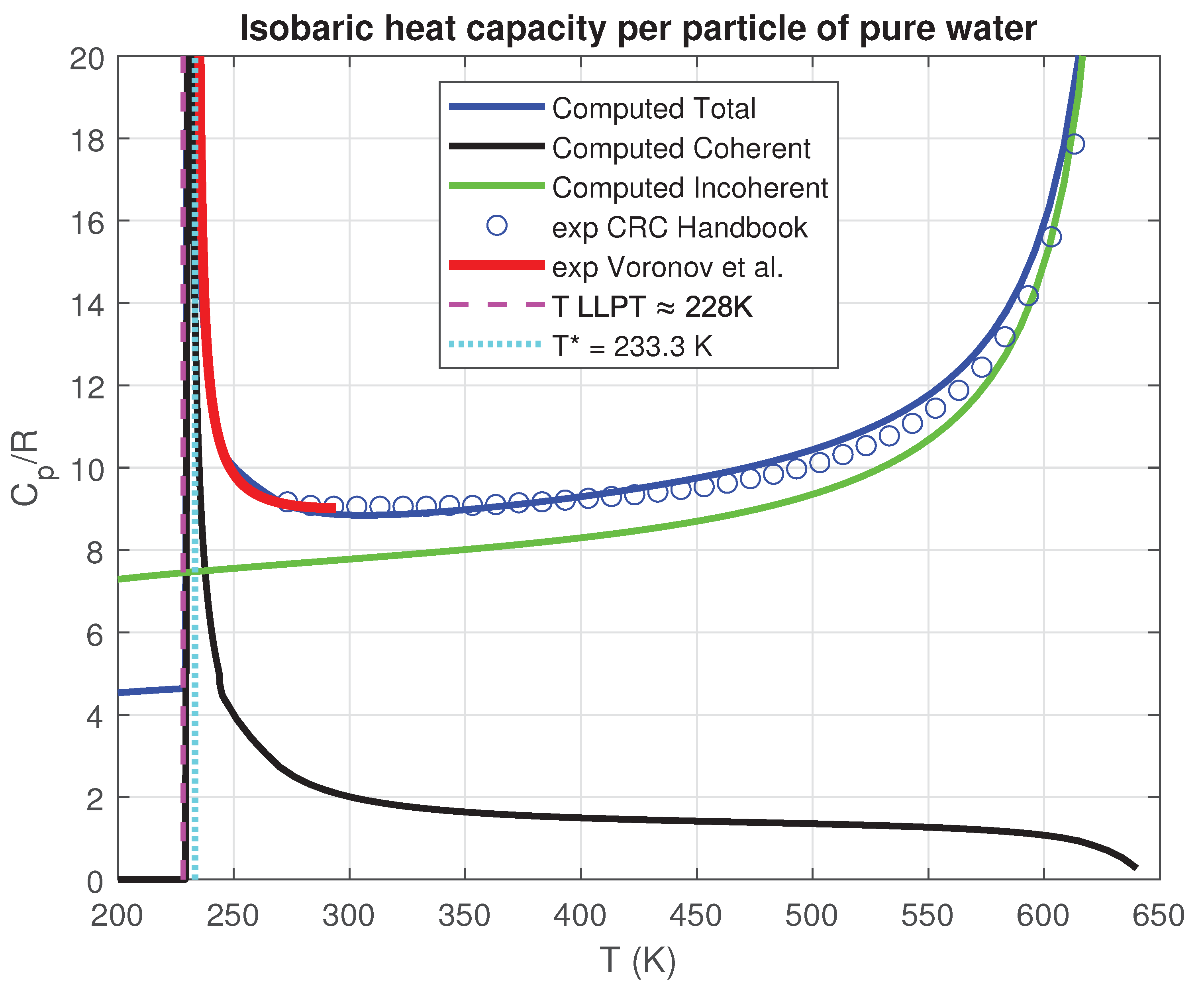
Figure 13.
Isothermal compressibility of liquid water as a function of temperature along the coexistence curve. A minimum is observed, consistent with the experimental observations.
Figure 13.
Isothermal compressibility of liquid water as a function of temperature along the coexistence curve. A minimum is observed, consistent with the experimental observations.
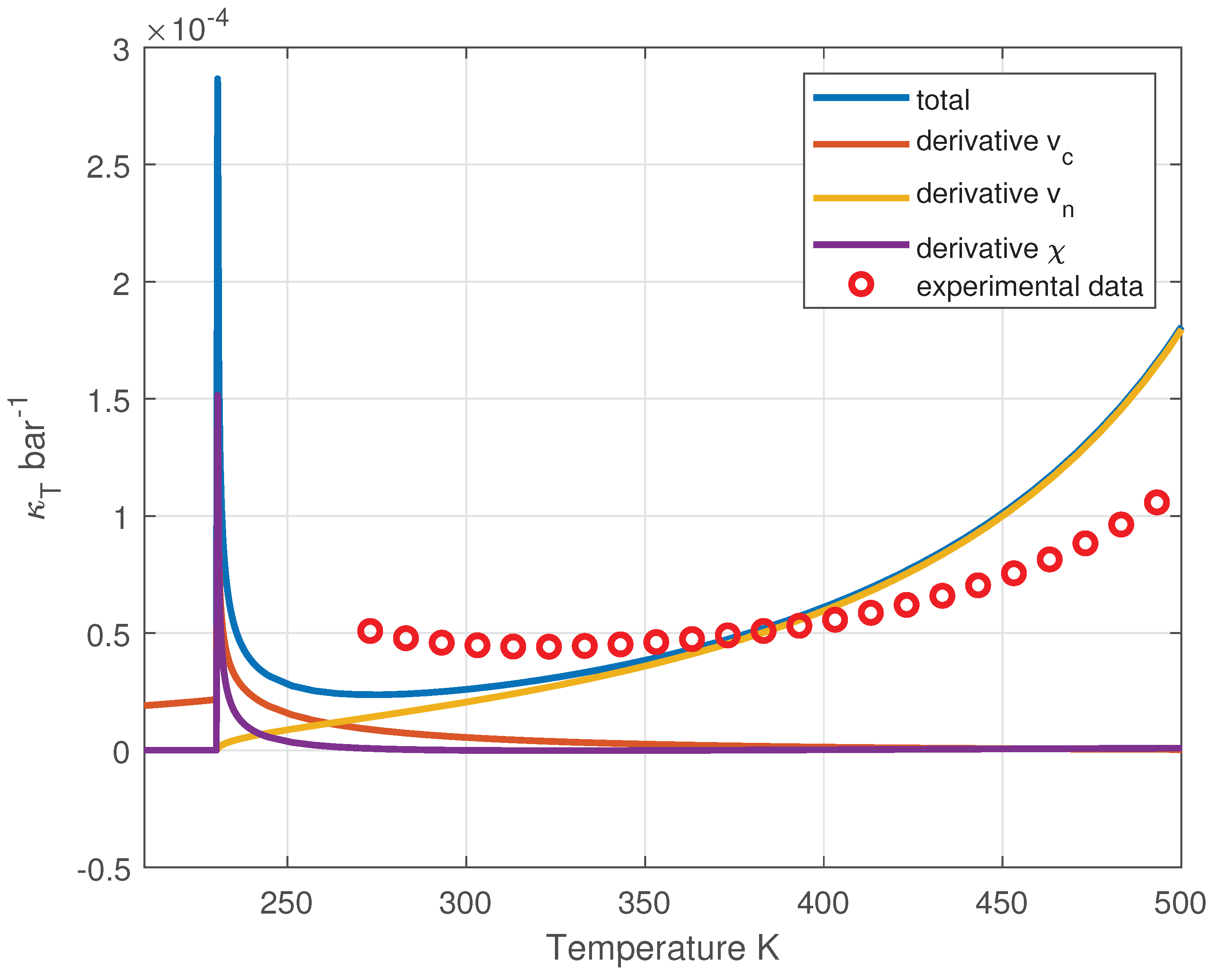
Figure 14.
Static dielectric constant of liquid water as a function of temperature along the liquid-vapor coexistence curve.
Figure 14.
Static dielectric constant of liquid water as a function of temperature along the liquid-vapor coexistence curve.
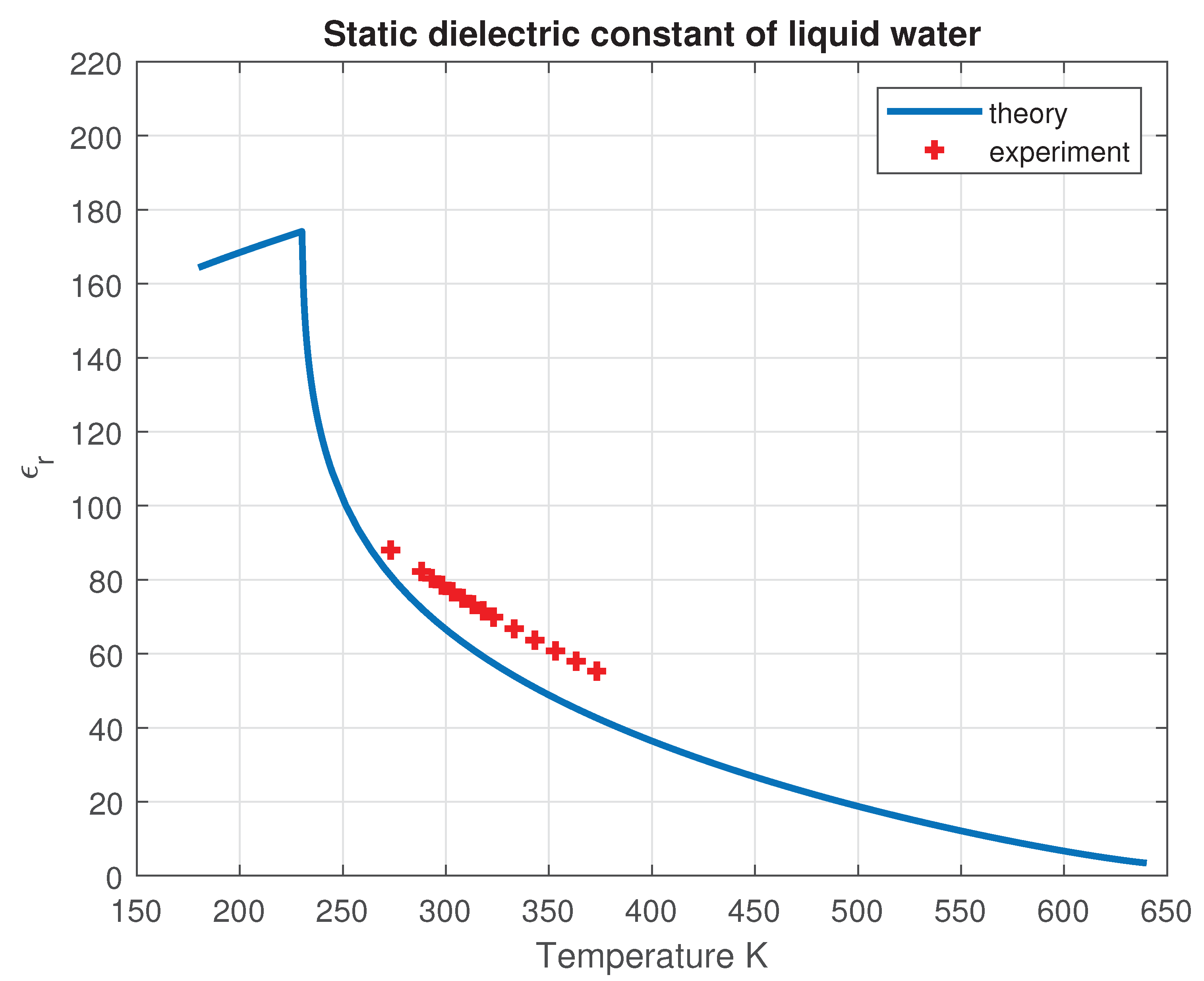

Table 1.
Principal vibrational modes of the coherent fraction with corresponding spectral weights and energies.
Table 1.
Principal vibrational modes of the coherent fraction with corresponding spectral weights and energies.
| Wavenumber (cm−1) | Spectral weight | Energy (meV) |
|---|---|---|
| 52 | 0.61 | 6.5 |
| 161 | 4.39 | 20 |
Table 2.
Parameter values and their respective units.
| Parameter | Value | Units |
|---|---|---|
| electric dipole for vapor | 1.84 | D |
| mass of water molecule | eV | |
| 0.0554 | eV | |
| (fit parameter) | ||
| reference coherent density (fit parameter) | ||
| coherent energy gap (fit parameter) | eV | |
| (fit parameter) | 0 | - |
| (fit parameter) | 0.2 | eV |
| (fit parameter) | 0.066 | eV |
Table 3.
Experimental values of .
| eV | |
|---|---|
| 7.400 | 0.0500 |
| 9.700 | 0.0732 |
| 10.000 | 0.0052 |
| 10.170 | 0.0140 |
| 10.350 | 0.0107 |
| 10.560 | 0.0092 |
| 10.770 | 0.0069 |
| 11.000 | 0.0218 |
| 11.120 | 0.0223 |
| 11.385 | 0.0098 |
| 11.523 | 0.0086 |
| 11.772 | 0.0178 |
| 12.074 | 0.0101 |
| 12.243 | 0.0053 |
| 12.453 | 0.0025 |
Disclaimer/Publisher’s Note: The statements, opinions and data contained in all publications are solely those of the individual author(s) and contributor(s) and not of MDPI and/or the editor(s). MDPI and/or the editor(s) disclaim responsibility for any injury to people or property resulting from any ideas, methods, instructions or products referred to in the content. |
© 2025 by the authors. Licensee MDPI, Basel, Switzerland. This article is an open access article distributed under the terms and conditions of the Creative Commons Attribution (CC BY) license (http://creativecommons.org/licenses/by/4.0/).
Copyright: This open access article is published under a Creative Commons CC BY 4.0 license, which permit the free download, distribution, and reuse, provided that the author and preprint are cited in any reuse.


