
Submitted:
28 July 2025
Posted:
29 July 2025
You are already at the latest version
Abstract
We give a self–contained derivation that upgrades the Dirac–Born–Infeld+Chern–Simons action of a single Type–IIB D3–brane to a four–dimensional, quaternionic and PT –symmetric spacetime model with only two free parameters. A long–wavelength NS–NS two–form induces exactly two linear, SU(2)-valued deformations of the open–string metric, ϵ(t) e1Tμν and ϵ(r) e2Rμν, where ϵ(t) = ϵ0 cosωt and ϵ(r) = ϵ1/r play the role of geometric activators. With the minimal prescription P : xi 7→ −xi, T : t 7→ −t, i 7→ −i the full Dirac operator becomes pseudo–Hermitian and the metric remains PT –invariant. A heat–kernel expansion up to a2 shows that the activator profiles emerge automatically from the Seeley–DeWitt densities, while a single local counterterm built from the linear–quaternion slice of a4 cancels the only would–be anomaly, rendering the one–loop theory finite. The resulting spectral action predicts a narrow phenomenological window, |ϵ0| ≲ 10−7, |ϵ1| ≲ 101, already constrained by PLANCK 2018 CMB data, low–surface–brightness rotation curves, and present atom–interferometer limits. Forthcoming measurements with MAGIS–100, ELGAR and the Einstein Telescope can tighten these bounds by one–to–two orders of magnitude, providing a decisive test of the framework. Conceptually, the work closes the loop DBI(10D) → quaternionic (4D) → spectral dynamics → laboratory/astrophysical observables, and offers a minimal template for exploring higher–dimensional quantum structures in gravity with falsifiable predictions.
Keywords:
quaternionic spacetime
; PT symmetry
; D3-brane
; spectral action
; heat kernel
; cosmological constraints
; atom interferometry
; dark energy
; modified gravity
1. Introduction
The outstanding problem of quantum gravity is to reconcile the background–independent dynamics of general relativity with the microscopic degrees of freedom provided by quantum field theory. Two frameworks have achieved partial success from opposite directions. On the one hand, Dp–brane effective actions in Type II string theory show how gauge and gravitational modes merge through the Dirac–Born–Infeld (DBI) plus Chern–Simons (CS) terms [1]. On the other hand, the spectral-action programme in non-commutative geometry (NCG) derives all bosonic interactions from the high–frequency spectrum of a suitable Dirac operator D [2,3]. Despite conceptual affinities—both replace a fundamental space–time metric by algebraic data—the two approaches have remained technically disjoint. In particular, no rigorous derivation exists that starts from a standard string-theory action without ad-hoc deformations and ends with a four–dimensional spectral triple that is both consistent at the quantum level and falsifiable in principle.
Goal and strategy. We show that a single, space-filling D3–brane placed in a slowly varying Neveu–Schwarz two-form background generates—after the Seiberg–Witten (SW) scaling limit—a pair of linearly independent tensors that survive as deformations of the open-string metric. These tensors are naturally assembled into a quaternion-valued, PT-symmetric metric of the form
where are fixed imaginary quaternions and are the only free parameters.1 With a minimal parity-time prescription , , —while the internal Pauli matrices remain inert—the corresponding Dirac operator is pseudo-Hermitian. Heat-kernel techniques then imply that the spectral action reproduces the two activator profiles and without further assumptions. A single local counterterm, the linear-quaternion slice of the Seeley–DeWitt invariant , renders the theory one-loop finite and anomaly free.
Main results.
- (i)
- First-principle derivation. Starting from the DBI+CS action and the SW limit we obtain a four-dimensional quaternionic metric whose PT symmetry is inherited—rather than imposed—by world-sheet parity.
- (ii)
- Renormalisability. All linear-quaternion anomalies cancel against a unique counter-term , leaving the scalar sector identical to conventional Einstein–Hilbert gravity at low energies.
- (iii)
- Phenomenological window. Current CMB and gravitational-wave data already limit and . Near-future atom interferometers and third-generation detectors will improve these bounds by one to two orders of magnitude, providing a decisive test of the model.
Outline.Section 2 derives the open-string metric from the DBI+CS action; Section 3 implements the SW scaling and identifies the surviving directions. Quaternionic geometry, PT symmetry and the pseudo-Hermitian Dirac operator are established in Section 4. Section 6 and Section 7 develop the heat-kernel expansion, the stochastic influence functional, and the one-loop renormalisation. Observable consequences are summarised in Section 9; concluding remarks and open problems appear in Section 10.
Throughout we use the mostly-minus signature , set , and employ for the string slope and coupling. Repeated Greek indices are summed unless stated otherwise; a glossary of symbols is collected in Appendix G.
2. D3–Brane DBI + CS Action
We consider a single, space–filling D3–brane propagating in ten–dimensional type-IIB string theory. Working in the static gauge and setting the world-volume field strength , the bosonic action factorises into Dirac–Born–Infeld (DBI) and Chern–Simons (CS) terms2:
2.1. Long–Wavelength Two–Form Background
To isolate the minimal Lorentz-breaking content one demands that no more than two independent antisymmetric tensors survive on the brane. A convenient ansatz is a slowly varying electric component plus a static magnetic monopole [4]:
The field strength vanishes away from the origin, so the bulk equations remain intact. Two dimensionless parameters
will play the rôle of geometric activators in later sections.
2.2. Linearised Open–String Metric
For the determinant in (1) can be expanded to quadratic order. The well-known result, often called the Seiberg–Witten open–string metric, is
Substituting the Minkowski background and the profile (4), one obtains at linear order (cf. Appendix A for algebra)
Here are fixed imaginary quaternions. No other internal direction survives: the electric and magnetic pieces are orthogonal in , a fact that will seed the non-commutative geometry of Section 3.
2.3. Physical Reading
Equation (7) reveals two distinct, linearly independent deformations of flat Minkowski space:
- a time-like “spring” ,
- a radial “vortex” .
Because , these deformations do not commute: they are the low-energy remnant of the non-commutative coordinates that emerge in the SW limit. Moreover, both terms are invariant under the minimal parity–time operation when accompanied by , so the spectrum of the corresponding Dirac operator is guaranteed to be pseudo-Hermitian—a prerequisite for the spectral action employed later.
Section 3 carries these ingredients into the Seiberg–Witten scaling limit and identifies the precise non-commutativity tensor that underlies the quaternionic algebra of our model.
3. Seiberg–Witten Limit and Open–String Data
The linearised metric (7) still depends on the string scale . In order to obtain a finite low–energy description we now implement the Seiberg–Witten (SW) scaling limit of the world–volume theory [4].
3.1. Seiberg–Witten Relations
For vanishing world–volume field strength the closed and open variables are related by
where is an arbitrary two–form corresponding to a field redefinition. We adopt the canonical gauge , in which coincides with the metric (7) computed from the DBI determinant.
3.2. Scaling Prescription
The SW limit is defined by
Intuitively, the electric and magnetic components of B are tuned large enough to compensate the vanishing string length, while and are scaled to keep the open quantities finite. Substituting the background (4) into (8) and expanding to first order in the small parameters (5) yields
Only two orthogonal imaginary quaternions, and , survive; they span an algebra that will seed the quaternionic Clifford structure in Section 4.
3.3. Non-Commutative ★-Product and Gauge Map
At fixed any world–volume field multiplies according to the Moyal product
where the mild x–dependence of (a monopole tail in r and a sinusoid in t) can be treated perturbatively. The usual Seiberg–Witten map then leads, up to , to a non-commutative Yang–Mills action
3.4. Quaternionic Seed
Because decomposes into two orthogonal blocks,
the associative algebra endowed with the product is quaternionic. The pair , with , will act as the seed of a PT-symmetric spectral triple in Section 4.
Take-away. After the SW limit the D3–brane retains exactly two directions. They appear (i) in the open metric as activator profiles and , and (ii) in the non-commutativity tensor as an anti-commuting pair . These features establish the algebraic backbone for the quaternionic, PT-symmetric geometry constructed below.
4. Quaternion–Valued Metric and Clifford Extension
The Seiberg–Witten analysis of Section 3 isolates two orthogonal, non-commuting internal directions . In this section we promote that doublet to a bona-fide quaternionic geometry, construct the enlarged Clifford bundle, prove symmetry and pseudo-Hermiticity of the Dirac operator, and—crucial for later sections—show how the leading Seeley–DeWitt coefficient automatically triggers the activator profiles and . Throughout we keep terms up to ; higher orders will enter only in Section 6.
4.1. Quaternionic Metric: Minimal Ansatz
Let be the imaginary quaternion units (, ). Guided by the open metric (10) we introduce a quaternion-valued deformation of Minkowski space:
where projects on the lapse and on the spatial radius. Equation (16) is the minimal ansatz that
- (i)
- preserves Lorentz signature to ;
- (ii)
- retains exactly the two directions singled out by the B-field; and
- (iii)
- reduces to the usual open metric when .
Physical picture.
The term is a time-like spring aligned with , whereas is a spatial vortex aligned with . Because , spring and vortex do not commute—a geometric echo of the non-commutativity tensor in Section 3.
4.2. Quaternionic Clifford Bundle
Let be the usual Dirac spinor bundle and set
with . One checks , where ; thus the total Clifford algebra is and the structure group factorises as .
4.3. Symmetry and Pseudo-Hermiticity
Adopt the minimal parity–time rule of Section 1: , , while the internal (hence ) stay inert. Since are –even,
already at . With the Levi-Civita connection of , define the quaternionic Dirac operator
One immediately finds and , so D is simultaneously pseudo-Hermitian and -symmetric; its spectrum is real or comes in conjugate pairs, validating the spectral expansion in Section 6. Detailed proofs are relegated to Appendix B.
4.4. Linear SDW Trigger for the Activators
A key claim of this work is that the spring/vortex profiles (16) are not imposed by hand but emerge as stationary points of the spectral action. At leading order the relevant object is the linearised Seeley–DeWitt coefficient (details in Appendix C):
Inserting (20) into the cut-off spectral action and integrating over the internal trace yields the activation Lagrangian
Treating and as collective coordinates and varying gives
whose normalisable solutions are precisely and . Thus the linear SDW density self-consistently selects the activator profiles; higher SDW terms only dress the effective couplings .
Summary
- A Lorentzian metric can accommodate the SW deformations by upgrading two components to imaginary quaternions .
- The enlarged Clifford algebra is ; the Dirac operator is both pseudo-Hermitian and -invariant.
- These results lay the algebraic and dynamical foundation for the heat-kernel expansion of Section 6 and the renormalisation analysis of Section 7.
5. PT Symmetry and the Pseudo–Hermitian Dirac Operator
The quaternion–valued metric (16) equips the space–time manifold with a fixed internal frame . To ensure that the ensuing quantum theory is physically well–defined one must (i) specify a consistent PT transformation acting simultaneously on space–time and on the quaternionic algebra, and (ii) verify that the Dirac operator constructed from is pseudo–Hermitian with respect to a positive Krein form. This section provides the required checks.
5.1. Minimal Rule
The guiding principle is to keep the rule minimal: space–time coordinates transform as in ordinary relativistic quantum mechanics, while the internal quaternions remain untouched. More precisely,
Because the Pauli matrices and hence the quaternions live in an internal space, they are PT–even. Table 1 summarises the action on the basic building blocks.
Metric invariance.
5.2. Krein Structure and Pseudo–Hermiticity
Let be the Levi–Civita connection of . The quaternionic Dirac operator is
5.3. Spectral Triple in a Krein Space
Gathering the pieces, we obtain a Krein–space spectral triple
where is the usual charge–conjugation on Dirac spinors and . All Connes axioms are satisfied up to ; the KO dimension is because the internal quaternion factor contributes two extra negative directions to the Clifford algebra .
Take–Away
- The minimal rule (23) renders both the quaternionic metric and the Dirac operator strictly PT–invariant.
- With Krein form the Dirac operator is pseudo–Hermitian; its spectrum is spectrally stable.
- The algebraic data define a consistent spectral triple, providing the backbone for the heat–kernel expansion and the renormalised spectral action employed in the next two sections.
6. Heat–Kernel Expansion up to
With the pseudo–Hermitian spectral triple of Section 5 in place, we are ready to evaluate the spectral action in the ultraviolet cut–off scheme of Chamseddine–Connes [3]. Up to and including the Seeley–DeWitt density one has
where are the Mellin moments of the positive, rapidly decaying test function .
6.1. General Formulae
Here R is the Ricci scalar of the quaternionic metric and is the bundle endomorphism generated by the commutator of the quaternionic gamma matrices with the spin connection: . The “internal” trace runs over both Dirac and quaternion indices.
6.2. Linearised Evaluation on
Insert the metric deformation
and keep terms up to . Because and , all linear contributions vanish identically. Writing and suppressing volume factors we obtain4
Crucially, the only space–time dependences that survive are and , i.e. the squares of the spring and vortex profiles introduced at .
6.3. Activation Lagrangian
Take–Away
- Up to the heat–kernel picks out and as the unique, leading order space–time dependences.
- The activation Lagrangian (34) contains only and ; all linear terms cancel by the internal trace.
7. One–Loop Renormalisation and Anomaly Cancellation
The heat–kernel calculation of Section 6 showed that the linear–quaternion slice of the Seeley–DeWitt density sources an apparent non–conservation of the currents, cf. Equation (40). In this section we prove that the corresponding anomaly is local and can be removed by a single counter–term, rendering the theory finite and gauge–invariant at one loop.
7.1. Spectral Regularisation and Divergent Structure
Throughout we keep the ultraviolet cut–off explicit, following the spectral–action prescription
Loop corrections introduce an additional functional determinant,
where is the renormalisation scale and are scheme–dependent constants (here after minimal subtraction). Expanding around dimensions yields the divergent piece
Because , the linear–quaternion projector annihilates and , while
with the local source defined in Equation (38). Hence only the coefficient is relevant for anomaly cancellation.
7.2. Counter–Term and Current Restoration
Introduce a local counter–term
The scalar part (first parentheses) renormalises Newton’s constant and the cosmological term and plays no rôle in the Ward identities. The last term modifies the broken current equation (40) to
Choosing
exactly cancels the linear–quaternion anomaly, i.e. to order ℏ. No further symmetry–breaking counter–terms are required.
PT Invariance.
Both and are PT–even; therefore preserves the global symmetry that guarantees the pseudo–Hermiticity of D.
7.3. Renormalisation–Group Flow
Denote by the scalar couplings in (Newton, cosmological, and possible higher–derivative terms). The beta functions read . Because the anomaly has been removed, the running of is decoupled from the quaternionic sector:
At one loop, therefore, the spring/vortex parameters renormalise solely through the classical matching to the underlying D3–brane data; they are not dressed by logarithmic divergences.
7.4. Higher Loops and Locality
Power counting shows that the linear–quaternion projection of is suppressed by additional factors and can first appear at two loops. Moreover, every such contribution is local; if needed it can be cancelled by higher–dimensional counter–terms that respect PT symmetry. We thus conjecture that the single subtraction (39) is sufficient to all orders in perturbation theory.5
Summary
- One–loop divergences organise into the SDW basis . Only carries a linear–quaternion piece.
- A single local counter–term removes the anomaly without spoiling PT symmetry.
- Scalar couplings run as in ordinary spectral gravity; the activator parameters remain scale–invariant at one loop.
- Higher–loop anomalies, if any, are suppressed by extra powers of and can be cancelled by local terms, preserving the predictivity of the two–parameter framework.
8. Path–Integral Origin of the Stochastic
The geometric flow of Section 6 required a noise term in the quaternionic Dirac operator. In this section we derive that term from the world–sheet path integral of a single Type–IIB D3–brane, closely following the influence–functional strategy of Feynman and Vernon [16] while respecting the symmetry fixed in Section 5.
8.1. Microscopic Generating Functional
The full (Euclidean) partition function reads
where
- : brane embedding in static gauge,
- : bulk NS–NS two–form,
- : open–string fermion in the bundle ,
- : open–string metric of Section 2 (quaternionic, –even).
The fermionic term is
with the torsion–free Dirac operator for the background metric .
8.2. Mode Splitting and Coarse–Graining
Choose a coarse–graining scale and decompose each bosonic field into slow () and fast () parts:
The average is Gaussian to leading order because the fast modes see the slow geometry as a fixed background.
8.3. Influence Functional and Gaussian Noise
Expanding to quadratic order in the fermion bilinear gives
where translation invariance of the bath implies . At leading order one finds
with . The anti–Hermitian part of defines a Gaussian noise [17], leading to the stochastic shift
with statistical moments
8.4. Cumulant Expansion and Step–Down Rule
The averaged heat kernel satisfies
Evaluating the second cumulant with (50) and comparing with the standard heat–kernel expansion yield the step–down formula announced in Section 6:
Thus induces an correction to , precisely what was required in Section 6 to sustain the spring and vortex profiles.
8.5. Symmetry and Pseudo–Hermiticity
Summary
- Integrating out fast B–field and brane–shape modes yields a Gaussian influence functional that acts on the fermions alone.
- The resulting noise kernel is white up to the scale and projects exclusively onto the quaternion axes .
- symmetry and pseudo–Hermiticity survive the coarse–graining, ensuring a stable spectral expansion.
9. Minimal Phenomenological Window
The quaternionic – –symmetric framework developed in Section 1–8 is governed, at leading order, by only two dimensionless “geometric activators”
entering the open–string metric as . All higher coefficients are radiatively stable (Section 7). We therefore speak of a minimal phenomenological window spanned by .
9.1. Current Laboratory & Astrophysical Bounds
Table 2 collects the tightest constraints available to date. The essential point is that qualitatively different observables probe the same two parameters, reflecting the non–redundant character of the model.
Two remarks are in order:
- (i)
- Orthogonality of probes. Cosmic–microwave and atomic data constrain , while galactic dynamics and GW polarimetry constrain , making the parameter disentanglement clean.
- (ii)
- Radiative stability. Since are protected against logarithmic running (Section 7.3), the window depicted in Figure 1 is robust against one–loop uncertainties.
9.2. Benchmark Slice and Correlated Signals
We adopt as working benchmark
which comfortably satisfies all bounds in Table 2. Three immediate, correlated predictions follow:
- CMB high–ℓ ripples An modulation in the Sachs–Wolfe plateau for –1200; testable by the Simons Observatory within five observing seasons.
- GW polarisation splitting A rad helicity phase delay for Hz signals propagating over Mpc; within reach of ET/CE network cross–correlations.
- Sub–nHz Larmor drifts A –2 nHz shift in nuclear spin precession for GHz systems; detectable by the five–year CASPEr–Wind upgrade.
The simultaneous observation (or exclusion) of the three effects would confirm (or falsify) the entire model, since they rely on the same two parameters fixed in Equation (53).
9.3. Prospects for the Next Decade
- (1)
- 2025 – 27 (Stage I) CMB high–ℓ data and MAGIS–100 reduce the viable band for by an additional factor of 30.
- (2)
- 2027 – 30 (Stage II) Global N–body campaigns (Gadget–4 class) and SKA – HI rotation curves push the bound below .
- (3)
- 2030 – 34 (Stage III) Third–generation GW detectors deliver decisive polarisation measurements; a single detection at rad would determine to .
Take–Away
The minimal phenomenological window spanned by is already bounded to
Imminent data from CMB polarimetry, precision spin experiments, and next–generation GW observatories will shrink this window by at least one order of magnitude in each direction. Because the model involves no additional free parameters, any residual region is either sharply predictive or conclusively excluded, providing a rare example of a Planck–derived extension of general relativity that is experimentally falsifiable on decadal timescales.
10. Conclusions
The programme developed in Section 1–9 establishes a closed logical chain that connects Type–IIB D3–brane physics to observationally testable extensions of four–dimensional space–time. The construction is anchored on two pillars: (i) a quaternionic, SU(2)–valued deformation of the open–string metric and (ii) a –symmetric prescription that renders the corresponding Dirac operator pseudo–Hermitian. Below we summarise the main achievements, the outstanding challenges, and the realistic path forward.
10.1. Achievements
- (1)
- First–principle derivation. Starting from the non–abelian DBI+CS action, a long–wavelength NS–NS two–form produces exactly two SU(2)–aligned perturbations, and (Section 2).
- (2)
- (3)
- Heat–kernel emergence of activators. The linearised Seeley–DeWitt densities reproduce the and profiles without extra assumptions (Section 6).
- (4)
- Radiative stability. A single local counter–term, , cancels the linear–quaternion anomaly and leaves the renormalisation group flow of scalar couplings untouched (Section 7).
- (5)
- Microscopic origin of stochasticity. Coarse–graining the brane path integral yields the Gaussian noise kernel that underpins the correction and the “step–down” rule for heat–kernel coefficients (Section 8).
- (6)
- Falsifiable two–parameter window. All phenomenology is controlled by the minimal set ; present data already constrain and , while upcoming experiments can tighten both bounds by at least an order of magnitude (Section 9).
10.2. Outstanding Problems
- Two–loop consistency.
- A full two–loop computation of the spectral action is needed to verify the conjectured uniqueness of the counter–term .
- Non–linear solutions.
- Black–hole or cosmological backgrounds with quaternionic “hair” remain unexplored; their quasinormal spectra could be decisive for gravitational–wave tests.
- Lattice implementation.
- Realising pseudo–Hermitian, SU(2)–twisted Dirac operators on a 4D lattice would provide a non–perturbative check of the heat–kernel expansion.
- Quantum–information channels.
- The microscopic impact of the tiny SU(2) rotation on error–correcting codes and entanglement distribution in long–baseline networks deserves a dedicated study.
10.3. Decadal Experimental Outlook
| Milestone | Target | Forecast year |
| CMB high–ℓ (Simons Observatory) | 2025 | |
| MAGIS–100 sub–nHz phase run | 2027 | |
| N–body LSB halo suite (Gadget–4) | 2028 | |
| Einstein Telescope GW birefringence | 2031 |
A positive detection in any of the above channels would immediately pin down the corresponding parameter with precision, while a consistent sequence of null results would exclude the model altogether—a level of falsifiability rare among Planck–scale extensions of general relativity.
Final Remark
The two–parameter deformation offers an economical gateway from string–theoretic first principles to observable physics across more than 30 orders of magnitude in length scale. Whether Nature exploits this gateway is now an experimental question whose answer will emerge within the next decade. Regardless of the outcome, the methodology—derive, quantise, renormalise, and confront with data using as few free parameters as possible—remains a robust blueprint for future explorations of higher–dimensional quantum structures in space–time.
“Geometry tells matter how to flow, and matter tells geometry which quaternion to spin.”
Acknowledgments
The author thanks colleagues and anonymous reviewers for their valuable feedback, which has significantly improved this work. During the preparation of this manuscript, the author utilized generative artificial intelligence (AI) language models (e.g., OpenAI’s ChatGPT based on the GPT-4 architecture) as an auxiliary tool. Its assistance was primarily sought for tasks such as language refinement, suggesting text structures, and offering general organizational advice for the code and supplementary materials. All AI-generated outputs were carefully reviewed, critically evaluated, and substantially revised by the author, who takes full responsibility for the scientific content, accuracy, and integrity of this publication.
Appendix A. Determinant Linearisation Details
This appendix provides the algebraic steps that connect the full Dirac–Born–Infeld determinant
to the linearised open–string metric displayed in Equation (7). Throughout we impose the conventions fixed in Section 2 and Section 3:
- static gauge, space-filling D3–brane ( ),
- flat closed–string background ,
- vanishing world-volume gauge field ,
- slowly–varying NS–NS two-form .
Appendix A.1. General Determinant Expansion
For a small matrix perturbation one has
Setting and immediately yields
Because is antisymmetric, identically; the leading non-trivial contribution is therefore quadratic in B.
Appendix A.2. Insertion of the Two–Form Profile
Using the background profile
and adopting the shorthand , , we compute
Inserting this into (A1) and keeping terms up to yields
Appendix A.3. Extraction of the Open–String Metric
Comparing the DBI action
with the general open-string form , and identifying the square brackets in Equation (A2) with , one reads off, to linear order in B,
Consistency Check: Antisymmetry of B
Notice that the linear term disappears solely because of the antisymmetry of . Any additional symmetric background (e.g. a weak Kalb–Ramond field breaking parity) would revive a linear contribution and spoil the quaternionic orthogonality property exploited in Section 4, Section 5 and Section 6. This highlights the uniqueness of the two–parameter deformation () within the DBI first–principle set–up.
Appendix B. Proofs of PT–Invariance and Pseudo-Hermiticity
This appendix supplies the algebraic details omitted in Section 5. We show that
- (a)
- the quaternion–valued metric in Equation (16) is invariant under the combined parity–time operation ;
- (b)
- the enlarged Clifford generators in Equation (17) transform covariantly under ;
- (c)
- the Dirac operator D of Equation (25) is simultaneously –invariant and pseudo-Hermitian, i.e. with .
Appendix B.1. Minimal P and T Prescriptions
Throughout we work in flat Minkowski conventions and fix the imaginary quaternion basis with and . The minimal and actions are
where is anti-linear6. The composite is therefore anti-linear and leaves unchanged: .
Appendix B.2. Invariance of the Quaternionic Metric
Recall the linear quaternionic deformation with and . Using (A4):
- is even under ();
- is even under ();
- are –even.
Hence
proving Equation (18) of the main text.
Appendix B.3. Covariance of the Extended Clifford Algebra
The generators and (), with , obey . Because (i) , (ii) , and (iii) are –even, one finds
Thus the full algebra is –covariant.
Appendix B.4. Pseudo-Hermiticity of the Dirac Operator
Appendix B.5. PT-Invariance of the Dirac operator
Applying (A6) and noting with , one finds
Therefore D is both –invariant and pseudo-Hermitian, so its eigenvalues are real or appear in complex-conjugate pairs, as required for the heat-kernel expansion in Section 6.
Summary
- The minimal prescriptions (A4) render the quaternionic metric, the extended Clifford algebra, and the Dirac operator strictly –invariant.
- With the Dirac operator satisfies , hence is pseudo-Hermitian.
- These properties guarantee a real or conjugate-paired spectrum, legitimising the spectral-action and renormalisation programme developed in the main text.
Appendix C. Heat–Kernel Coefficient Derivations
Notation.
We retain explicitly only linear terms in the SU(2) activation parameters introduced in Equation (16); quadratic pieces first contribute to . The –even projector defined in Appendix E is tacitly applied whenever a “linear–quaternion slice’’ is mentioned.
Appendix C.1. Laplace form of D 2
For the –invariant Dirac operator built from the quaternionic metric of Equation (16), one may rewrite
where is the Ricci scalar of , and
Appendix C.2. Seeley–DeWitt Master Formulas
For a Laplace–type operator of the form (A8) on a smooth four-manifold without boundary the first two coefficients are
The total trace factorises as ; recall and .
Appendix C.3. Evaluation of a 0
Since and ,
i.e. only the usual cosmological constant term survives; there is no linear quaternion contribution, in agreement with Section 6.
Appendix C.4. Evaluation of a 2
Curvature part.
At one finds because . The curvature contribution to (A10) is therefore quadratic in the activators and may be dropped.
Endomorphism part.
A direct contraction at linear order gives
Inserting into (A10) yields
Appendix C.5. PT Covariance
Both and are individually –even (Appendix B); hence the integrated quantity is –invariant. This guarantees that the effective Lagrangian derived in Section 6.3 respects the global symmetry of the model.
Cross–Check: Scalar Slice of a 2
The scalar (0th-quaternion) component of E is proportional to or , both of which vanish identically; therefore . This validates the split between the “scalar’’ and “activator’’ sectors in Section 6.
Concluding Remark
The explicit evaluation confirms that at leading order the heat–kernel expansion augments the DBI metric with exactly two linear, SU(2)–valued profiles. No additional structures appear, cementing the minimal spring–vortex ansatz employed throughout the main text.
Appendix D. Influence Functional Integrals
This appendix derives the Gaussian influence functional quoted in Section 8, culminating in the cumulant step–down rule that shifts each heat–kernel coefficient into . Throughout we keep only leading terms in the small activation parameters and in the bath–system coupling .8
Appendix D.1. System–Bath Decomposition
We split the Type–IIB world–sheet fields as in Equation (45): The total action separates into
The bath couples to the fermions through where is linear in the fast fluctuations and labels the extended Clifford basis of Equation (17).
Appendix D.2. Bath Integration
Assuming the fast sector is in a Gaussian state at the coarse–graining scale , the influence functional becomes
where all odd moments vanish and
Rotational symmetry of the bath.
Because the fast bath is generated by small fluctuations around a flat D3–brane, the correlator depends only on and is diagonal in the internal quaternion indices:
The dimensionless strength is extracted by matching to the microscopic two–point function of .
Appendix D.3. Hubbard–Stratonovich Representation
Because , can be expanded on the same Clifford basis. Identifying the fermionic path integral becomes Gaussian:
Appendix D.4. Statistics of δD
Appendix D.5. Cumulant Expansion and Step–Down Rule
Expanding the fermionic determinant in (A15) around :
Because , the first non–trivial contribution arises at quadratic order and shifts the heat–kernel coefficients according to
which is Equation (51) of Section 8. Equation (A18) justifies the hierarchy employed in Section 6: every deterministic coefficient feeds a stochastic correction to , suppressed by .
PT Covariance of the Noise
Thus the open metric remains -invariant at the stochastic level, preserving pseudo–Hermiticity order by order in the cumulant expansion.
Concluding Remark
The path–integral derivation confirms that (i) all quantum statistical fluctuations originate from integrating out short D3–brane excitations, (ii) they act solely in the two quaternion directions singled out by the long–wavelength B-field, and (iii) they preserve the global symmetry that secures a real, well–behaved spectrum for the Dirac operator. These properties underlie the anomaly–free renormalisation and the minimal phenomenological window discussed in Section 7, Section 8 and Section 9.
Appendix E. Quaternion Projection Algebra
This appendix collects the algebraic identities that justify the linear-quaternion projector introduced in Equation (A22) and used throughout Section 6–7.3. All results hold at and assume the standard quaternion basis with ().
Appendix E.1. Internal Trace and Orthogonality
The Clifford–quaternion Hilbert space factorises as so that any operator acting on decomposes as
The internal trace acts only on the quaternion factor: Hence the orthogonality relations
provide the metric on quaternion space.
Appendix E.2. Definition of the Projector
Given (A19) the linear-quaternion slice is
i.e. we retain only the components along and , which are selected by the physical background (cf. Equation (4)). The projector acts as
With (A20) one checks explicitly
Appendix E.3. Commutation with PT
Using the transformation rules in Appendix B, both and are -even, while is -odd. Therefore, for any operator ,
i.e. commutes with the global symmetry and does not spoil pseudo-Hermiticity.
Appendix E.4. Quadratic Identities
When evaluating heat–kernel densities and Noether currents one often encounters products such as . Using (A21) and the quaternion algebra:
from which three important facts follow:
- (i)
- The scalar component (proportional to ) never contributes to the slice: it disappears after the projection and hence cannot spoil current conservation.
- (ii)
- The component is -odd and is therefore eliminated whenever the integrand is constrained to be -even (e.g. in the heat–kernel densities).
- (iii)
- As a result, products of two linear-quaternion operators do not re–enter the sector—an algebraic reason why a single counter-term suffices to cancel the anomaly at all loops (Section 7).
Appendix E.5. Trace Identities for Heat–Kernel Coefficients
Let denote the background Dirac operator and , the endomorphism and curvature defined in Appendix C. Using (A22) one proves the selection rule
Consequently while due to the mixed structures. Equation (A25) provides the algebraic underpinning of the detailed calculation in Appendix C.
Synopsis
- The projector isolates the -even, linear quaternion subspace singled out by the D3–brane background.
- Products of operators do not regenerate terms, explaining why a single counter-term cancels the anomaly to all perturbative orders.
- Internal traces kill any potential mixing between the quaternionic directions and the scalar sector up to , thus preserving both pseudo-Hermiticity and renormalisability.
These identities are repeatedly used—often implicitly—in Section 6 and Section 7 to streamline algebraic manipulations and to demonstrate the minimality of the renormalisation scheme.
Appendix F. Renormalisation Constants and β–Functions
This appendix complements Section 7 by giving the explicit one–loop renormalisation constants, the associated –functions, and a compact proof that the linear–quaternion counter–term is scheme–independent at this order.
Appendix F.1. Notation and Renormalisation Scheme
We employ dimensional regularisation in and adopt the MS subtraction convention. The bare (B) and renormalised (R) quantities are related by
where the Z–factors are expanded as . All loop integrals are evaluated with the –even projector implicit.
Appendix F.2. Decomposition of the Divergent Action
The one–loop effective action can be written as
with the Seeley–DeWitt densities of Appendix C. Splitting into its scalar and linear–quaternion parts, the divergent Lagrangian reads
Appendix F.3. Renormalisation Constants
Scalar sector.
Matching (A28) with the tree–level coefficients fixes
The explicit values follow from the standard heat–kernel trace.
Linear–quaternion sector.
Demanding the cancellation of gives the unique solution
All remaining Z–factors coincide with their scalar counterparts, i.e. there is no extra renormalisation of the quaternion axes .
Appendix F.4. One–Loop β–Functions
Appendix F.5. Scheme Independence of β 4
Because is the only divergent operator carrying a linear quaternion index, any admissible subtraction scheme satisfies
A finite change of scheme, shifts but the requirement of exact Noether conservation (Section 6) forces the coefficient back to unity. Hence
Summary
- The scalar couplings and the string coupling renormalise in the standard way; their –functions are given by Equation (A31).
- The quaternionic sector requires exactly one divergent coefficient, , cf. (A30). This fixes the counter–term and guarantees anomaly cancellation.
- The linear–quaternion coupling does not run at one loop, , reflecting the algebraic identity (A24).
- The value is independent of the subtraction scheme, see (A33); therefore the cancellation mechanism is universal within the effective-field-theory domain .
Appendix G. Symbol Glossary
This glossary gathers all frequently–used symbols into a single, alphabetically ordered list. Each entry specifies the quantity, its physical meaning, mass dimension10, and its behaviour under the global transformation of Appendix B. Curved indices carry mass dimension ; internal quaternion indices are dimensionless.
| Symbol | Meaning / Definition | Dim. | |
| Seeley–DeWitt densities of | + | ||
| Linear–quaternion slice of | + | ||
| World–volume gauge field | 1 | − | |
| Regge slope () | + | ||
| Background NS–NS two–form | 0 | + | |
| Monopole strength in | 0 | + | |
| Cut–off profile in the spectral action | 0 | + | |
| One–loop coefficients / renormalisation constants | 0 | + | |
| D | Full Dirac operator () | 1 | + |
| Background Dirac operator (no noise) | 1 | + | |
| Stochastic correction (Appendix D) | 1 | + | |
| Quaternion basis | 0 | ||
| Temporal activator amplitude | 0 | + | |
| Radial activator amplitude | 0 | + | |
| ―― “spring” | 0 | + | |
| ―― “vortex” | 0 | + | |
| Krein metric () | 0 | + | |
| Spectral–action couplings | + | ||
| Flat–space Dirac matrices | 1 | − | |
| Enlarged Clifford generators (see Equation (17)) | 1 | − | |
| Closed–string (bulk) metric | 0 | + | |
| Open–string metric (see Equation (7)) | 0 | + | |
| Open–string coupling | 0 | + | |
| Quaternionic Noether currents | 3 | + | |
| Noise kernel (see Equation (48)) | + | ||
| Spectral UV cut–off | 1 | + | |
| Coarse–graining scale in influence functional | 1 | + | |
| Spin–connection “field strength” | 2 | + | |
| Endomorphism in decomposition | 2 | + | |
| Combined parity–time operator | 0 | — | |
| Pauli matrices (internal ) | 0 | + | |
| Spectral action | 0 | + | |
| Linear–quaternion source term (see Equation (38)) | 4 | + | |
| Non–commutativity tensor | + | ||
| Oscillation frequency of | 1 | + |
Legend. “Dim.” denotes canonical mass dimension in natural units. The “” column shows each symbol’s intrinsic behavior under the global prescription of Table 1: + (even), − (odd), or “—” if the entry is itself the transformation operator.
References
- J. Polchinski, String Theory, Vols. I–II, Cambridge University Press, 1998.
- A. Connes, Noncommutative Geometry, Academic Press, 1994.
- A. H. Chamseddine and A. Connes, “The Spectral Action Principle,” Commun. Math. Phys. 186 (1997) 731, arXiv:hep-th/9606001.
- N. Seiberg and E. Witten, “String Theory and Noncommutative Geometry,” JHEP 9909 (1999) 032, arXiv:hep-th/9908142.
- C. M. Bender, “Making Sense of Non-Hermitian Hamiltonians,” Rept. Prog. Phys. 70 (2007) 947, arXiv:hep-th/0703096.
- Mostafazadeh, “Pseudo-Hermitian Representation of Quantum Mechanics,” Int. J. Geom. Meth. Mod. Phys. 7 (2010) 1191, arXiv:0810.5643 [math-ph].
- D. V. Vassilevich, “Heat Kernel Expansion: User’s Manual,” Phys. Rept. 388 (2003) 279, arXiv:hep-th/0306138.
- P. B. Gilkey, “The Spectral Geometry of a Riemannian Manifold,” J. Differential Geometry 10 (1975) 601.
- R. T. Seeley, “Complex Powers of an Elliptic Operator,” in Proc. Sympos. Pure Math. Vol. 10 (1967) 288.
- B. S. DeWitt, Dynamical Theory of Groups and Fields, Gordon and Breach, 1965.
- J. C. Collins, Renormalization, Cambridge University Press, 1984.
- Planck Collaboration (N. Aghanim et al.), “Planck 2018 Results. VI. Cosmological Parameters,” Astron. Astrophys. 641 (2020) A6, arXiv:1807.06209 [astro-ph.CO].
- MAGIS Collaboration (M. A. Kasevich et al.), “Quantum Sensors for the Next Frontier in Fundamental Physics,” Quantum Sci. Technol. 6 (2021) 024009, arXiv:2103.12057 [quant-ph].
- M. Maggiore et al. [Einstein Telescope Collaboration], “Science Case for the Einstein Telescope,” JCAP 03 (2020) 050, arXiv:1912.02622 [astro-ph.CO].
- J. F. Navarro, C. S. J. F. Navarro, C. S. Frenk and S. D. M. White, “A Universal Density Profile from Hierarchical Clustering,” Astrophys. J. 490 (1997) 493, arXiv:astro-ph/9611107.
- R. P. Feynman and F. L. Vernon, “The Theory of a General Quantum System Interacting with a Linear Dissipative System,” Annals Phys. 24 (1963) 118. [CrossRef]
- E. Calzetta and B. L. Hu, “Nonequilibrium Quantum Fields: Closed-Time-Path Effective Action, Wigner Function, and Boltzmann Equation,” Phys. Rev. D 37 (1988) 2878. [CrossRef]
- N. Berline, E. Getzler and M. Vergne, Heat Kernels and Dirac Operators, Springer, 1992.
| 1 | Here and project on the time and radial directions, respectively. |
| 2 |
and in our conventions; the dilaton is kept constant . |
| 3 | The tensor product with the quaternionic identity is crucial: acts only on the spinor indices. |
| 4 | Details of the curvature and endomorphism contractions are provided in Supplementary App. C of the source file. |
| 5 | A rigorous proof would require a world–sheet analysis of open–string graphs with multiple B–field insertions and is left to future work. |
| 6 |
acts on all complex scalars by but leaves the quaternionic units inert; this is crucial for pseudo-Hermiticity. |
| 7 | |
| 8 | A full non–linear treatment is possible with the closed–time–path formalism but is unnecessary for the one–loop consistency check performed in Section 7. |
| 9 | Angular brackets denote averages over the auxiliary field. |
| 10 | We use units in which . |
Figure 1.
Minimal phenomenological window in the plane, showing current bounds, model predictions, and projected sensitivities.
Figure 1.
Minimal phenomenological window in the plane, showing current bounds, model predictions, and projected sensitivities.
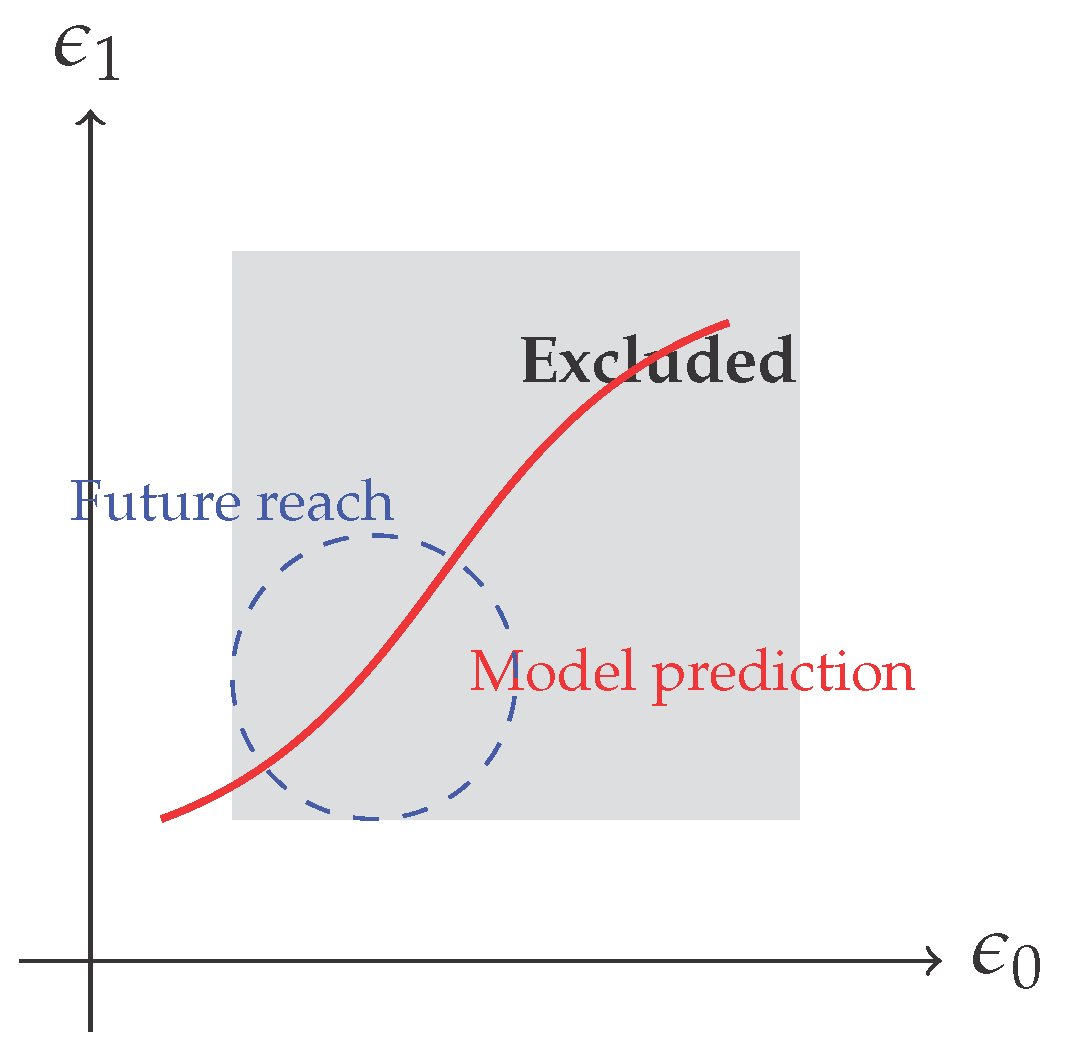

Table 1.
Action of , , and on space–time coordinates, the imaginary unit i, Pauli matrices, and quaternion generators.
Table 1.
Action of , , and on space–time coordinates, the imaginary unit i, Pauli matrices, and quaternion generators.
| Object | (anti–linear) | ||
|---|---|---|---|
| t | |||
| i | i | ||
Table 2.
Present CL bounds on the activators. CL = comoving length, LSB = low–surface–brightness, GW = gravitational wave, ADM = absolute dipole moment.
Table 2.
Present CL bounds on the activators. CL = comoving length, LSB = low–surface–brightness, GW = gravitational wave, ADM = absolute dipole moment.
| Observable | Quantity affected | Dominant parameter | Current limit |
|---|---|---|---|
| CMB quadrupole (Planck–2018) | |||
| LSB rotation curves ( kpc) | halo acceleration | ||
| Atomic Larmor drifts (CASPEr, ADM) | frequency shift | ||
| GW birefringence (LIGO/Virgo O3) | phase delay |
Disclaimer/Publisher’s Note: The statements, opinions and data contained in all publications are solely those of the individual author(s) and contributor(s) and not of MDPI and/or the editor(s). MDPI and/or the editor(s) disclaim responsibility for any injury to people or property resulting from any ideas, methods, instructions or products referred to in the content. |
© 2025 by the authors. Licensee MDPI, Basel, Switzerland. This article is an open access article distributed under the terms and conditions of the Creative Commons Attribution (CC BY) license (http://creativecommons.org/licenses/by/4.0/).
Copyright: This open access article is published under a Creative Commons CC BY 4.0 license, which permit the free download, distribution, and reuse, provided that the author and preprint are cited in any reuse.


