
Submitted:
24 July 2025
Posted:
28 July 2025
You are already at the latest version
Abstract
As consumer awareness grows and regulations regarding the quality and safety of perishable goods become stricter, careful management of environmental conditions throughout the supply chain is becoming essential. Among these factors, storage temperature plays a crucial role in preserving the physicochemical characteristics of products.Therefore, an effective approach to ensure quality and safety up to the final customer is to continuously monitor the temperature within warehouses, using specific location-mapping techniques and stocking optimisation methods. This study proposes a dynamic optimization model for the Storage Location Assignment Problem (SLAP), integrating both temperature and humidity constraints into the placement of stock-keeping units (SKUs). The model operates under a multi-period, multi-product framework and leverages real-time sensor data to account for spatial temperature stratification and environmental variability within the warehouse. Two alternative optimization strategies are explored: one focused on minimizing thermal and humidity stress, and another targeting the reduction of average storage cycle time. A detailed what-if analysis is conducted across three scenarios, varying warehouse fill rates and incoming load volumes, in order to prove the effectiveness of the proposed model in real-data context.
Keywords:
cold warehounsing
; storage assignment
; optimisation
; temperature control
; humidity control
1. Introduction
Over recent decades, global food trade has increasingly addressed consumer concerns about the so-called credence attributes—aspects like quality, safety, sustainability, and fair-trade practices [1]. Events such as food safety scandals have heightened public sensitivity and boosted consumer demand for transparency and adherence to strict standards [2].
Environmental factors including temperature, humidity, and vibrations significantly influence the shelf life and sensory qualities (such as taste and freshness) of perishable goods like food and pharmaceuticals [3]. Managing these conditions effectively is especially critical at storage points such as warehouses, where products remain for extended periods [4]. Among these environmental variables, temperature [6] and humidity [5] are widely recognized as the most critical factor in safeguarding product integrity. Numerous studies have shown that poor temperature control leads to chemical and physical degradation, accelerating spoilage and compromising safety. Consequently, regulatory bodies have developed safety and quality standards to guide companies in ensuring proper storage conditions during distribution [7]. Moreover, the phenomenon of air stratification in the storage area and the facility’s structural features of refrigerated warehouses (such as insulation quality, exposure to sunlight, and internal layout) reduce the effectiveness of storage zones in maintaining safe conditions for the stock-keeping units (SKUs) [21].
Monitoring the temperature conditions in warehouses is considered a best practice. Therefore, quality managers are typically required to conduct temperature mapping to track fluctuations over time and different techniques were proposed in the past under this perspective [6]. These techniques are fast evolving in the era of Industry 5.0, where temperature monitoring in logistics and warehousing has become increasingly sophisticated and data-driven [8]. Advanced technologies such as Internet of Things (IoT) sensors, wireless data loggers, and real-time monitoring systems are now commonly employed to continuously track temperature conditions throughout the supply chain. These devices transmit data to cloud platforms, enabling predictive analytics and proactive decision-making. Under this perspective, optimization techniques play a pivotal role in enhancing the efficiency and responsiveness of storage and retrieval operations within refrigerated warehouses. These environments demand precise coordination to minimize energy consumption, reduce product handling time, and maintain strict temperature control, all while ensuring rapid access to perishable goods. Leveraging AI-driven algorithms, digital twins, and real-time data analytics enables dynamic decision-making that optimizes warehouse layout, routing of autonomous vehicles, and inventory rotation strategies [9]. This not only improves operational sustainability but also enhances worker safety and adaptability, aligning with the core principles of Industry 5.0—collaboration between humans and machines for resilient and value-driven logistics. [10,29].
In warehousing, optimizing the assignment of SKUs to storage locations is a well-recognised critical activity for improving the overall performance and responsiveness of warehouse operations [19]. Strategic SKU placement directly impacts picking efficiency, travel time, and inventory accessibility, especially in high-throughput environments. Moreover, an intelligent SKU assignment strategy helps balance workload across different zones, avoids congestion, and supports more accurate space utilization. This becomes even more essential in dynamic inventory settings, where demand patterns fluctuate and real-time adaptability is required [20]. These aspects become more relevant within refrigerated warehouses.
Proper placement of SKUs not only improves picking efficiency and reduces travel time, but also ensures that sensitive items are stored in zones with the most appropriate environmental conditions, taking under control temperature and humity. For instance, products with stricter thermal requirements can be positioned closer to more stable cooling zones, while less sensitive goods may be stored in peripheral areas. This strategic allocation helps maintain consistent climate conditions by minimizing unnecessary door openings, reducing air circulation disruptions, and limiting exposure to external temperatures [21]. Additionally, optimizing SKU locations reduces energy consumption by supporting better airflow and reducing the workload on refrigeration systems. In this way, intelligent SKU-to-location mapping contributes not only to operational efficiency but also to the sustainability and regulatory compliance of cold chain logistics [22].
This paper advances the cold warehousing literature on the storage assignment problem by introducing an original dynamic optimization model for the allocation of perishable products. The model is inspired by a real refrigerated warehouse used by a company operating in the cold food chain, for storing frozen foods, considering a stocking area with capacity of 5000 food-grade plastic pallets (referred as unit loads in the following). The refrigerated storage area has recently undergone modernization and has been equipped with sensors capable of detecting the warehouse’s temperature and humidity levels in real time, for mapping the temperature profile. The company aims to leverage this information to improve the storage process of incoming load units. To this scope, the proposed model integrates both temperature and humidity control into the decision-making process for SKUs placement on storage racks. Additionally, a what-if analysis is conducted through a case study to evaluate the impact of storage decisions driven by environmental control considerations.
The remainder of the paper is arranged as follows: Section 2 organizes a review of the literature; Section 3 illustrates the optimisation model, Section 4 showcases the methodology with a case study and introduces computational results, as well as, and Section 5 presents the study’s conclusions and provides goals for further research developments.
2. Materials and Methods
Within refrigerated warehouses, the typical storage and retrieval operations are influenced by several factors related to the specific boundary conditions. Below, a detailed overview will be provided of the studies addressing these conditions and those combining such considerations with SKUs storage strategies.
2.1. Perishable Products Storage Conditions
Within the food industry, improper control of warehouse temperature and humidity accelerates microbial growth and causes physical degradation of products—altering flavour, texture, and appearance [11]. Two key indicators are commonly used to monitor quality: shelf life, which measures the period during which a product retains acceptable quality (also known as stability period), and the Freshness Gauge, which evaluates freshness based on remaining shelf life [5]. Accurate determination of shelf life is critical for setting expiration and sell-by dates.
Indoor climate conditions also affect worker health and productivity, further highlighting the need for precise environmental control in industrial storage spaces [12]. A major challenge is air stratification, where temperature gradients develop vertically in high-ceiling warehouses, leading to inefficient heating and non-uniform temperatures [13,14,15].
The warehouse layout - along with elements such as skylights, loading docks, and fan airflow - can exacerbate thermal imbalances. Although computational fluid dynamics has been suggested to simulate these environments [17], it is often impractical due to cost and complexity. Instead, many facilities use temperature mapping with data loggers to empirically assess how heat distribution varies over time and space. Temperature mapping involves monitoring how temperature levels change over time within storage environments, such as cold chambers, industrial refrigerators or warehouses. The goal is to ensure that the environmental conditions match the storage requirements specified for the products. This process helps detect temperature variations caused by structural characteristics, facility design or human activity. This method helps identify problem zones, even as external weather conditions change [6].
2.2. Storage Location Assignment Problem
One of the most critical challenges in warehouse management is the Storage Location Assignment Problem (SLAP) [23], which involves determining the optimal placement of items within a storage system to improve overall efficiency. Poor assignment strategies can lead to increased travel time, labor costs, and order picking delays [20]. SLAP is particularly complex due to the variety of constraints and objectives involved, such as minimizing retrieval times, balancing workload, and accommodating product-specific storage requirements. Several variants have emerged in the literature, including random assignment, class-based assignment, and volume-based assignment. Random assignment offers simplicity but sacrifices efficiency [25], while class-based methods group items by demand frequency to improve pick performance (e.g., assigning fast-moving SKUs closer to dispatch zones). More advanced approaches include correlated storage [24], where items frequently ordered together are stored nearby to minimize picker travel distance. Optimization-based solutions often rely on heuristics, metaheuristics (e.g., genetic algorithms), or integer programming to solve these problems under realistic constraints. Recent studies have also explored dynamic assignment models [21], which adjust item locations over time based on evolving demand patterns and warehouse usage. These dynamic methods are increasingly relevant in fast-paced environments such as e-commerce or cold chain logistics, where adaptability is key to maintaining service levels and operational efficiency.
Unlike conventional settings, SLAP in cold storage environments must account not only for operational efficiency but also for product-specific temperature and humidity requirements, shelf-life constraints, and energy optimization goals [26]. Objective functions in this context typically aim to minimize travel distance, reduce order picking time, and optimize energy usage by clustering goods with similar thermal profiles [21]. Some variants of SLAP incorporate thermal zoning strategies, assigning products to storage zones based on their sensitivity to temperature fluctuations, while others focus on first-expired-first-out (FEFO) policies to ensure product freshness [27]. Additionally, multi-criteria decision models may consider factors such as product turnover rate, weight, volume, and compatibility with other SKUs. Constraints often include limited space in cold zones, restricted access due to condensation or frost, and energy-intensive equipment operation schedules. More advanced formulations leverage mixed-integer programming or metaheuristics to balance competing objectives [28], such as minimizing total retrieval time while adhering to strict cold chain compliance [30]. These specialized SLAP models are increasingly relevant in the management of pharmaceuticals, fresh products, and frozen foods, where preserving product integrity is as critical as achieving logistical efficiency. For a complete overview in the field, the reader can refers to the survey of Yurtseven et al. [22], Muhammad et al. [31] and Ren et al. [32].
2.3. Contribution to the Literature
This paper contributes to the literature proposing a storage location assignment problem with innovative characteristics, as an extension of the problem proposed in Baruffaldi et al. [6]. In particular:
- a multi-period SLAP model has been proposed for storage management over a specific planning horizon. This model is particularly suited to the dynamic nature of warehouses and allows for the management of refrigerated storage activities using simple rolling horizon approaches, while accounting for the variability of boundary conditions;
- the model features an objective function composed of two main terms: one related to maintaining the safety temperature, and the other related to humidity level. This characteristic is entirely novel within the class of SLAP problems, which often consider only temperature conditions, or focus on optimizing operational metrics such as time and energy reduction, without taking product quality into account;
- the model also accounts for the multi-product scenario, which reflects a realistic condition in warehouse management—particularly in refrigerated warehouses. In such contexts, the need to maintain the cold storage area at a suitable temperature, combined with the phenomenon of air stratification, often clashes with the specific and sometimes heterogeneous temperature requirements of different products;
- a real case-study is introduced, where the temperature measuring is provided by sensors, and a what-if-analysis is introduced for evaluating the storage-retrieval cycle efficiency and the quality considerations introduced into the model.
3. Mathematical Formulation
This section illustrates the SLAP optimization model designed to determine the best storage for incoming unit loads, using the temperature mapping data of a specific storage area. It concerns selecting the most appropriate storage location for an incoming pallet of a specific SKU, with the aim of optimizing a general convenience-related objective function.
The model is developed under the assumption that sensors provide data to a tool processing thermal loggers, to generate a detailed map of both historical and real-time indoor storage conditions. This enables the development of storage assignment models focused on reducing thermal stress on inventory throughout its lifecycle.
The rest of this section is dedicated to formalizing the multi-period multi-product storage location assignment problem (MPSLAP), where the quality of conservation conditions serves as the core criterion for the optimization process. The MPSLAP is modeled considering:
- the set I representing the storage locations in the stocking area;
- the set S introducing the different stock keeping units (SKUs);
- the set T describing the time horizon;
- the set representing an ordered list of unit loads, of different SKUs, to be stocked at each time . It can be partitioned as follows: , with . Note that represents the number of unit loads of type s to be stocked in period t.
The following parameters are considered:
- : temperature measured at location in period ;
- : safe temperature range for unit load and ;
- : humidity for unit load measured at the location ;
- : weight to scale the effect of humidity in comparison with temperature considerations, with ;
- : target humidity;
- : takes value 1 if the location is empty during period , 0 otherwise;
- : distance between the location and the optimal location for the unit load according to the highest safe temperature and the target humidity . This parameter pushes the assignment of the incoming unit loads according to the highest expected temperature stress that is measured in that location along a time horizon from t to . The term is the average period that a pallet is stored in the warehouse, computed considering historical data on SKU ;
- : expected stress temperature for unit load measured at the location during the starting from period .
Parameter is computed assuming that a storage location occupied until the corresponding SKU is removed, that is for periods, may be exposed to stress or critical temperature conditions that could compromise the load safe preservation. It is determined as follows:
Using (1) is possible to measure the highest stress temperature during the time frame ] for the unit load and location . The distance is consequently computed, as follows:
Note that, the closer the temperature is to the safe storage range for load , the more the configuration aligns with optimal storage conditions.
The unique set of decision variables is , that is a binary variable taking value 1 if the unit load is assigned to the location during the period , 0 otherwise. Then, the model is formulated as follows and solved with a rolling horizon approach [33], for each period :
The objective function (3) represents the quality preservation measuring how much the current storage setup deviates from the configuration that would minimize the stress temperature and the humidity slack from the target. Constraint (4) forces the assignment of load to a single storage location . Constraint (5) guarantees that each storage location is filled by a unit load only if location is empty. Constraint (6) shows the binary nature of the decision variables.
The objective of the model is to optimize the overall benefit derived from the periodically allocation of incoming unit loads to available storage locations. This benefit depends on the storage conditions observed at each location. By considering the maximum expected stress temperature at a given location over the time range and a humidity target, the model directs the assignment of unit load to the most suitable available location . It should be noted that the rolling horizon approach is applied through the update of the set of storage units to be allocated, and the parameter , which accounts for the positions that were occupied and those that have been emptied due to retrieval operations, in the period .
4. Computational Results
This section is dedicated to computational experiments. As aforementioned, the case study is inspired by a real stocking area of 5000 unit loads capacity, equipped with sensors for monitoring humidity and temperature. To this scope a what-if analysis is conducted considering four cases (called in the following as scenarios), on the basis of different settings of the and of the storage fill rate of the stocking area.
The what-if analysis is a decision-making tool used to evaluate the potential outcomes of different scenarios by changing input variables in a model, allowing to explore how variations in assumptions—such as cost increases, sales volume fluctuations, or resource changes—affect the final results. It is widely used in warehouse process simulations to evaluate how changes in variables—such as staffing levels or equipment configurations—affect operations. This approach enables organizations to optimize performance and make informed decisions without disrupting actual workflows [34].
The MPSLAP was implemented using Lingo 21.0 (https://www.lindo.com/), a powerful optimization software that supports various problem types, including mixed-integer programming. Lingo applies the branch-and-bound method for integer problems and enhances performance through preprocessing and cutting techniques for linear mixed-integer models, improving solution times. For more details, see the Lingo manual (https://www.lindo.com/downloads/PDF/LINGO.pdf, accessed July 4, 2025).
The computer used for the computational experiments is equipped with an AMD Ryzen 7 3700U with Radeon Vega Mobile Gfx processor, 8,00 GB of RAM, and Windows 11 Professional 64-bit.
4.1. Description of the Case Study
The considered storage area is characterized by the following features:
- , represents the capacity of the storage area, a building measuring meters along the x-axis and meters along the y-axis;
- the unit loads are handled with forklifts;
- the safe temperature range for the storage area is ;
- the target humidity chosen is ;
- the measured values for for unit load at the location i are within the interval .
- the parameter is set to a value of 0.6;
- random lists are generated for each scenario;
- one period of planning is considered in the time horizon;
- the parameter is assigned a value of 1 or 0 randomly, depending on the specific scenario considered, to show if the location i is empty or not respectively.
The warehouse operates under a "random storage policy", meaning that SKUs are dynamically assigned to storage locations based on current availability. As a result, the allocation of SKUs changes over time depending on the real-time occupancy of the storage space. This policy allows for maximum utilization of the available storage space. Each unit load u must be automatically identified - using any identification method - in order to continuously update the database of storage locations occupied by stored unit loads u. This update occurs at the end of every storage or retrieval operation.
The warehouse is structured into two blocks, each containing 20 aisles of selective racking, for a total of 40 storage locations arranged along the y-axis—two of which are positioned against the walls. Each shelving unit includes 25 storage locations along the x-axis and is divided into 5 vertical levels. Figure 1 shows a top view of the refrigerated storage area layout, indicating the front and the back courts. Note that the entrance door is positioned on the on the front court.
The parameters considered in the analysis are listed in Table 1. Each rack has a length . The width of a storage location is given by , so the width of a single row is . Accordingly, the total length of the storage area is and the total width of the storage area is .
Figure 2 visually illustrates the layout of the refrigerated warehouse, highlighting the temperature gradient that transitions from colder to warmer zones throughout the facility. Notably, it emphasizes the progressive temperature increase from the front—closer to the airflow source—toward the rear of the storage racks, a pattern primarily driven by diminished air circulation and localized heat accumulation, as well as from the air stratification from the floor to the top of the building. This thermal distribution is derived from on-site sensor data collected at various rack depths and heights, enabling a spatially resolved understanding of temperature dynamics. Such a thermal profile is instrumental for optimizing product placement by aligning storage zones with temperature stability, thereby ensuring the preservation of temperature-sensitive goods and enhancing overall energy efficiency.This technical illustration was developed in Autodesk Inventor, ensuring dimensional precision and realistic representation.
For each storage location, the time required to complete both the storage cycle and the retrieval cycle has been calculated. These times depend on the distance that the forklift must travel to reach the respective location. The storage time and the retrieval time are calculated as follows:
The what-if analysis is conducted considering three different scenarios, associated to variegate configurations of filling storage rate and number of incoming unit loads, as introduced in the following:
-
First scenario (S1). A progressive increase in warehouse occupancy levels was considered, based on a total of 5000 storage locations. Four different fill rates were analyzed: 20%, 40%, 60%, and 80%, while keeping the number of incoming unit loads constant (). Specifically:
- at 20% warehouse occupancy, 875 locations were already occupied and 4125 were available. After the placement of the 625 incoming unit loads, the number of free locations decreased to 3500;
- at 40% occupancy, 1750 locations were occupied and 3250 were available. After allocation, the number of free locations reduced to 2625;
- at 60% occupancy, 2625 locations were occupied and 2375 were available. After placement, free locations decreased to 1750;
- at 80% occupancy, 3500 locations were already occupied, leaving 1500 available. After adding the incoming unit loads, the remaining free locations were reduced to 875.
-
Second scenario (S2). In this case, the number of incoming unit loads was varied across four levels (250, 500, 750, and 1000) to assess the impact of load volume on warehouse operations, assuming a fixed warehouse occupancy rate of 50%. The following cases were considered:
- for 250 incoming unit loads, a total of 4750 storage locations were considered. Prior to their arrival, 2625 positions were available; following placement, 2375 remained free and 2375 were occupied;
- for 500 incoming unit loads, the total number of storage locations was 4500. Before placement, 2750 positions were available; afterward, 2250 remained free and 2250 were occupied;
- for 750 incoming unit loads, 4250 storage locations were considered. Initially, 2875 positions were available; after placement, 2125 remained free and 2125 were occupied;
- for 1000 incoming unit loads, the total number of storage locations was 4000. Before their arrival, 3000 positions were available; after allocation, 2000 remained free and 2000 were occupied.
-
Third scenario (S3). In this scenario, the number of incoming unit loads was set to 250, 500, 750, and 1000, while maintaining a fixed warehouse occupancy level of 50%, corresponding to 2500 free and 2500 occupied storage locations at the initial state. The outcomes for each case are as follows:
- With 250 incoming unit loads, the number of available storage locations decreased to 2250, while the number of occupied positions increased to 2750;
- With 500 incoming unit loads, the available storage locations decreased to 2000, and occupied positions increased to 3000;
- With 750 incoming unit loads, the available storage locations decreased to 1750, and occupied positions increased to 3250;
- With 1000 incoming unit loads, the available storage locations decreased to 1500, and occupied positions increased to 3500.
4.2. Description of the Computational Approach
The MPSLAP (3)–(6) is solved considering the three proposed scenarios under different warehouse conditions. The scope is to assess the importance of minimizing the distance between the target temperature and humidity target during the storage location process. Under this perspective, the storage cycle time for each stocked pallet () is considered, finally computing the average value for each time period (). This approach is referred as a posteriori analysis, for calculating the average storage cycle time. This method enables the evaluation of how distance-based storage allocation influences the duration of storage operations, assuming that locations with easier access are associated with shorter handling times. The approach involving the resolution of the model (3)–(6) is referred as in the following.
In order to provide a comparison of the adopted metric, a new version of the problem is solved. The objective function (3) is substituted by (9), where the distance component is replaced with the storage cycle time . The model (9), (4)-(6) is re-solved accordingly.
The purpose of the revised objective function (9) is to minimize the overall storage cycle time by directly optimizing the allocation of incoming products to storage locations. Subsequently, the average storage cycle time is computed. This formulation aims to promote storage locations that reduce handling distance, but also ensure faster product turnover. The approach involving the resolution of the model (9), (4)–(6) is referred as in the following.
Finally, for and and for each scenario, the barycentre for each is calculated. For the evaluation of barycentre the following features are considered:
- are the coordinates of the storage location ;
- represents the lengthwise position (i.e., the distance from the entrance) of the storage location ;
- represents the transverse position (i.e., the reference lane) of the storage location ;
- represents the vertical position (i.e., the shelf level) of the storage location .
The barycentre coordinates , for are computed as:
By analyzing the barycentre resulting from both allocation strategies, it becomes possible to evaluate how these approaches shape the spatial distribution of stored unit loads within the warehouse layout. The barycentre is calculated using the geometric coordinates of the assigned storage locations and acts as a spatial indicator of how centralized or dispersed the allocation is with respect to key reference points, such as the warehouse entrance or high-traffic zones. A more centralized barycentre may indicate a more efficient configuration, potentially reducing travel distances and handling times. Conversely, a more dispersed barycentre might reflect less efficient space utilization or a deliberate trade-off that prioritizes thermal stability over proximity to access points. Comparing the barycentres derived from distance-based and storage cycle-time-based optimization strategies allows for an assessment of how each method balances operational efficiency with cold chain integrity. This spatial perspective adds a valuable layer of analysis, revealing how model-driven decisions influence not only key performance metrics but also the physical deployment of goods across the warehouse grid. The results are summarized in the following subsections, one for each scenario.
4.2.1. Discussion of the Results
In the following, the results obtained for S1, S2 and S3 using two different approaches and are described. As aforementioned, the what-if-analysis is conducted on two main performance indicators: and barycentre.
4.2.2. Results for Scenario S1
Table 2 presents the average stock time values for four different sub-cases related to the increasing fill rate of the storage area (20%, 40%, 60%, and 80%) under scenario S1, using two different approaches: and . It is possible to observe that:
- approach consistently yields higher average stock times than approach across all cases.
- as the case percentage increases from 20% to 80%, there is a slight increasing trend in average stock time for both approaches, with values for ranging from 105.595 to 106.426, and for from 79.898 to 89.466 (see Figure 3).
Table 3 shows the coordinates of the barycentre for each sub-case related to the increasing fill rate of the storage area, under the same scenario S1, again comparing the two approaches and . For each case (20%, 40%, 60%, and 80%), a set of 3D coordinates is provided representing the central point (barycentre) of the positions assigned to the incoming unit loads. It is possible to observe that:
- the barycentre coordinates show that in case , the height is usually higher (around the third shelf level), while in case , it stays close to the floor. This is because the goal in case is to protect the temperature of the load units, so the model places pallets mostly in cooler areas.
- as the filling rate increases, it is possible to observe that the barycentre also shifts across the building floor plan, with varying degrees of significance. Specifically: in case , the barycentre shows slight fluctuations along the x and y-axis, always remaining in a central position within the building layout; in case , the barycentre moves significantly away from the entrance as the number of occupied positions increases.
- by observing the two barycentre plotted together in Figure 4, Figure 5, Figure 6 and Figure 7 for each sub-case, it can be seen that the approach based on minimizing total storage time (), which is the more traditional method, shifts the barycentre of the assigned positions closer to the entrance door. This exposes the load units to higher temperatures and greater fluctuations due to the door opening. The other approach, instead, which is based on a metric specifically designed for refrigerated scenarios, places the load units not too far from the door but still in significantly cooler areas.
4.2.3. Results for Scenario S2
As for the first scenario, Table 4 and Figure 8 compares the average for two different approaches, and , across four different sub-cases (250, 500, 750, 1000 number of units loads incoming). The results clearly indicate that the average increases parallelly with the increasing number of unit loads in approach , as expected, while, this effect is less evident in approach . This is due to the position of the barycentre that presents the same behaviour of the scenario S1 (see Table 5).
4.2.4. Results for Scenario S3
As for the previous scenarios, Table 6 and Figure 9 compares the average for two different approaches, and , across four different sub-cases (250, 500, 750, 1000 number of units loads incoming). The results clearly indicate that the average increases parallelly with the increasing number of unit loads in approach , as expected, while, this effect is less evident in approach . This is due to the position of the barycentre that presents the same behaviour of the scenario S1 (see Table 7).
4.3. Results Comparison
The analysis conducted under S1,S2,S3 highlights the trade-off between temperature-aware optimization and cycle time efficiency in refrigerated warehouse operations. The results show that , which prioritizes environmental conditions (temperature and humidity), consistently leads to higher average storage cycle times compared to Approach , which minimizes handling time.
For instance, as the number of incoming unit loads increased from 250 to 1000 (in S2 and S3), the average stock time under remained nearly constant (around 106 s), whereas under it steadily increased from around 77 s to around 89 s; as well as in S1 where the fill rate of the storage area progressively increases (20%, 40%, 60%, 80%) with a fixed number of incoming unit loads, average stock times range around 106 s under , while yields significantly lower values, from 79 s to 89 s.
Despite its higher cycle time, ensures improved product preservation by assigning unit loads to cooler and more stable storage zones, as demonstrated by the barycentre coordinates. placements are more centralized and higher along the z-axis, leveraging stratified cooler air, while tends to cluster goods near the entrance, exposing them to potential thermal fluctuations due to frequent door openings. These findings validate the proposed optimization model’s ability to integrate environmental metrics into storage decisions, showing that even a moderate sacrifice in operational speed can significantly enhance quality control for perishable goods.
5. Conclusions and Future Works
This study introduced a novel optimization model for the storage location assignment problem (SLAP) in refrigerated warehouses, integrating both temperature and humidity considerations into the decision-making process. One of the key strengths of the proposed model lies in its ability to enhance product preservation by explicitly minimizing environmental stress—rather than focusing solely on operational efficiency. The inclusion of a multi-period and multi-product framework, along with a temperature mapping strategy based on real sensor data, further improves the model’s applicability to real-world dynamic conditions.
Another strong point is the comparative analysis performed across three different warehouse scenarios, which demonstrates the model’s robustness and adaptability. The consistent spatial separation of barycentres between the two approaches ( and ) highlights how optimization criteria affect warehouse layout utilization and product exposure to thermal fluctuations. The approach , while slightly less efficient in terms of average storage time, shows superior performance in maintaining product quality through strategic placement.
In terms of research gaps, the current model does not account for stochastic demand patterns, inventory turnover policies such as FEFO or FIFO, or not random stocking policy, which are highly relevant in cold chain logistics. Moreover, energy consumption, although indirectly influenced, is not explicitly optimized in the current formulation. Additionally, the absence of real-time reallocation strategies limits its flexibility in highly dynamic warehouse settings.
Future developments could explore hybrid optimization approaches, combining the strengths of and by dynamically switching between quality-preserving and time-efficient allocation depending on SKU sensitivity, seasonality, or operational load. The integration of energy efficiency metrics and real-time adaptive control mechanisms (e.g., using machine learning or digital twins) would also significantly enhance the model’s practical impact and sustainability. Lastly, validating the model through field experiments in operational warehouses would be a crucial step toward industrial adoption and further refinement.
Author Contributions
Carlo Maria Aloe: conceptualization, software, validation, writing—original draft preparation. Annarita De Maio: conceptualization, methodology, formal analysis, writing—original draft preparation, supervision.
Funding
The work of Annarita De Maio was partially funded by the Ministry of Enterprises and Made in Italy under the research grant
Data Availability Statement
Data are available to the authors upon request.
Conflicts of Interest
The authors declare no conflicts of interest.
References
- Bernués, A., Olaizola, A., Corcoran, K., 2003. Extrinsic attributes of red meat as indicators of quality in Europe: an application for market segmentation. Food Qual. Prefer. 14 (4), 265–276.
- Marshall, D., McCarthy, L., McGrath, P., Harrigan, F., 2016. What’s your strategy for supply chain disclosure? MIT Sloan Manag. Rev. 57 (2), 37–45.
- Hertog, M.L.A.T.M., Uysal, I., Verlinden, B.M., Nicolaı, B.M., 2014. Shelf life modelling for first-expired-first-out warehouse management. Philos. Trans. R. Soc. A Math. Phys. Eng. Sci. 372.
- Meneghetti, A., Monti, L., 2014. Greening the food supply chain: an optimisation model for sustainable design of refrigerated automated warehouses. Int. J. Prod. Res. 7543, 1–21.
- Woo Ram Kim, Myo Min Aung, Yoon Seok Chang, Charalampos Makatsoris, Freshness Gauge based cold storage management: A method for adjusting temperature and humidity levels for food quality, Food Control, Volume 47, 2015, Pages 510-519.
- Giulia Baruffaldi, Riccardo Accorsi, Daniele Santi, Riccardo Manzini, Francesco Pilati, Chapter 9 - The storage of perishable products: A decision-support tool to manage temperature-sensitive products warehouses, Editor(s): Riccardo Accorsi, Riccardo Manzini, Sustainable Food Supply Chains, Academic Press, 2019, Pages 131-143.
- European Commission, C 343/1, 2013. Guidelines of 5 November 2013 on good distribution practice of medicinal products for human use. Off. J. Eur. Union. 23.11.2013, 2001–2024.
- M. Kosmidis, S. Antoniou, V. Balaska, I. Kansizoglou and A. Gasteratos, "Towards Warehouse 5.0: A Framework of Human-Centered Technologies," 2024 IEEE International Conference on Imaging Systems and Techniques (IST), Tokyo, Japan, 2024, pp. 1-6, doi: 10.1109/IST63414.2024.10759201.
- J. B. Montes, S. Z. Fernández and V. D. Casas, "Internet of Things in Energy-Sensitive Processes: Application in a Refrigerated Warehouse," in IEEE Access, vol. 12, pp. 76257-76276, 2024, doi: 10.1109/ACCESS.2024.3406992.
- Yanpeng Li, Yiwei Feng, Chuang Wang, Ziwen Xing, Dawei Ren, Lin Fu, Performance evaluation and optimization of the cascade refrigeration system based on the digital twin model, Applied Thermal Engineering, Volume 248, Part A, 2024, 123160,.
- Vaikousi, H., Biliaderis, C.G., Koutsoumanis, K.P., 2008. Development of a microbial time/temperature indicator prototype for monitoring the microbiological quality of chilled foods. Appl. Environ. Microbiol. 74 (10), 3242–3250.
- Rohdin, P., Moshfegh, B., 2011. Numerical modelling of industrial indoor environments: A comparison between different turbulence models and supply systems supported by field measurements. Build. Environ. 46 (11), 2365–2374.
- Armstrong, M., Chihata, B., MacDonald, R., 2009. Cold weather destratification energy savings of a warehousing facility. ASHRAE Trans. 115 (2), 513–518.
- Aynsley, R., 2005. Saving heating costs in warehouses. ASHRAE J. 47 (12), 47–51.
- Li, W., 2016. Numerical and experimental study of thermal stratification in large warehouses. April, 121 pp.
- Brinks, P., Kornadt, O., Oly, R., 2015. Air infiltration assessment for industrial buildings. Energy Build. 86, 663–676.
- Ho, S.H., Rosario, L., Rahman, M.M., 2010. Numerical simulation of temperature and velocity in a refrigerated warehouse. Int. J. Refrig. 33, 1015–1025.
- https://www.lindo.com/index.php/products/lingo-and-optimization-modeling.
- Islam, S.; Uddin, K. Correlated storage assignment approach in warehouses: A systematic literature review. "Journal of Industrial Engineering and Management", Setembre 2023, vol. 16, núm. 2, p. 294-318.
- Medrano-Zarazúa, L., Saucedo-Martínez, J.A., Bolaños-Zuñiga, J. (2024). Storage Location Assignment Problem in a Warehouse: A Literature Review. In: Marmolejo-Saucedo, J.A., Rodríguez-Aguilar, R., Vasant, P., Litvinchev, I., Retana-Blanco, B.M. (eds) Computer Science and Engineering in Health Services. COMPSE 2022. EAI/Springer Innovations in Communication and Computing. Springer, Cham. [CrossRef]
- R. Accorsi, G. Baruffaldi, R. Manzini, Picking efficiency and stock safety: A bi-objective storage assignment policy for temperature-sensitive products, Computers & Industrial Engineering, Volume 115, 2018, Pages 240-252,.
- Yurtseven, C., Ekren, B.Y., Toy, A.O. (2022). An Overview of Warehouse Operations for Cold Chain. In: Calisir, F. (eds) Industrial Engineering in the Internet-of-Things World. GJCIE 2020. Lecture Notes in Management and Industrial Engineering. Springer, Cham. [CrossRef]
- Solano Charris, E. L., & Montoya Torres, J. R. (2018). The Storage Location Assignment Problem: A Literature Review. International Journal in Industrial Engineering Computations, 199-224. [CrossRef]
- Ren-Qian Zhang, Meng Wang, Xing Pan, New model of the storage location assignment problem considering demand correlation pattern, Computers & Industrial Engineering, Volume 129, 2019, Pages 210-219. [CrossRef]
- Venkata Reddy Muppani (Muppant), Gajendra Kumar Adil, Efficient formation of storage classes for warehouse storage location assignment: A simulated annealing approach, Omega, Volume 36, Issue 4, 2008, Pages 609-618. [CrossRef]
- Jie Wang, Qiusen Wang, Peng Yang, Jie Yu, Li Xiao, Energy consumption analysis and optimization of cold stores considering differential electricity price, Energy and Buildings, Volume 310, 2024, 114094. [CrossRef]
- A. Mendes, J. Cruz, T. Saraiva, T. M. Lima and P. D. Gaspar, "Logistics strategy (FIFO, FEFO or LSFO) decision support system for perishable food products," 2020 International Conference on Decision Aid Sciences and Application (DASA), Sakheer, Bahrain, 2020, pp. 173-178, doi: 10.1109/DASA51403.2020.9317068.
- Zarinchang, A., Lee, K., Avazpour, I., Yang, J., Zhang, D., & Knopf, G. K. (2023). Adaptive warehouse storage location assignment with considerations to order-picking efficiency and worker safety. Journal of Industrial and Production Engineering, 41(1), 40–59. [CrossRef]
- Min, H. Smart Warehousing as a Wave of the Future. Logistics 2023, 7, 30. [CrossRef]
- Chen, Y.; Li, Y. Storage Location Assignment for Improving Human–Robot Collaborative Order-Picking Efficiency in Robotic Mobile Fulfillment Systems. Sustainability 2024, 16, 1742. [CrossRef]
- Muhammad Firdaus Mujibuddin Syah Mustafa, Namasivayam Navaranjan, Amer Demirovic, Food cold chain logistics and management: A review of current development and emerging trends, Journal of Agriculture and Food Research, Volume 18, 2024, 101343. [CrossRef]
- Ren, T.; Ren, J.; Matellini, D.B.; Ouyang, W. A Comprehensive Review of Modern Cold Chain Shipping Solutions. Sustainability 2022, 14, 14746. [CrossRef]
- Violi, A., De Maio, A., Fattoruso, G. et al. An age-based dynamic approach for distribution of perishable commodities with stochastic demands. Soft Comput 27, 7039–7050 (2023). [CrossRef]
- Mariagrazia Dotoli, Nicola Epicoco, Marco Falagario, Nicola Costantino, Biagio Turchiano, An integrated approach for warehouse analysis and optimization: A case study, Computers in Industry, Volume 70, 2015, Pages 56-69. [CrossRef]
Figure 1.
Top view of the refrigerated warehouse layout.
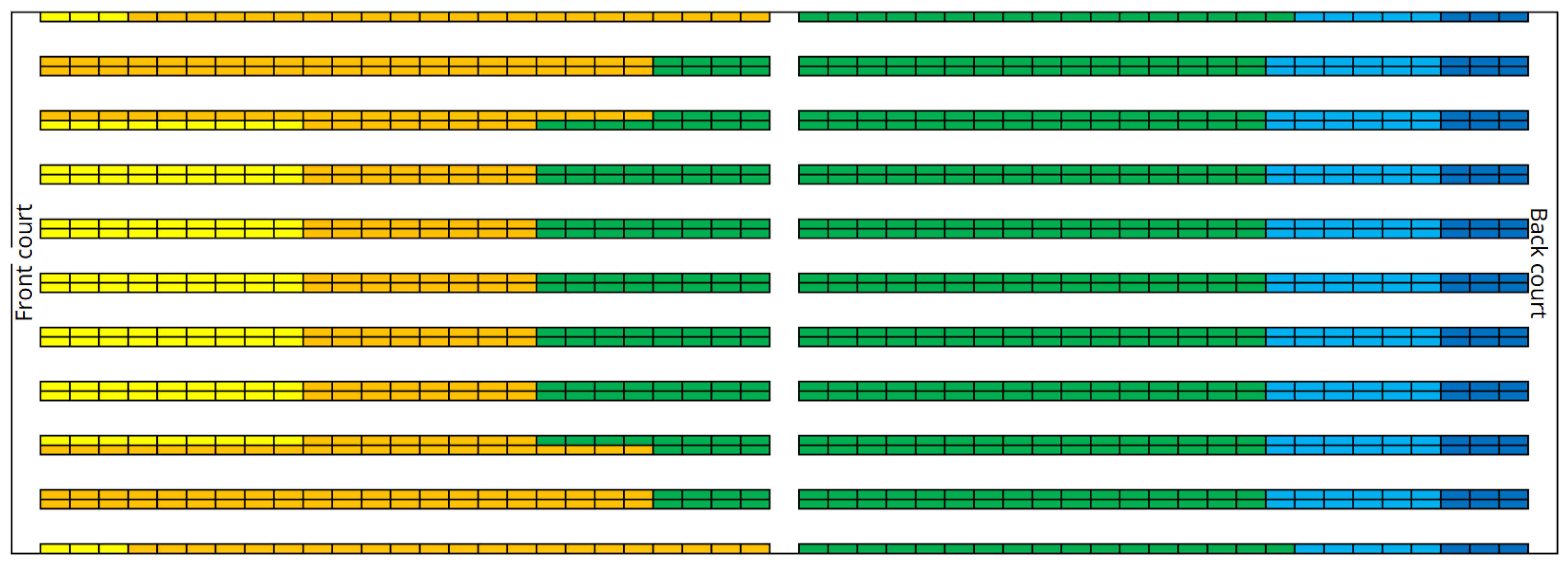
Figure 2.
3D model of the layout of the refrigerated warehouse with 5000 storage locations . (Image created using Autodesk Inventor).
Figure 2.
3D model of the layout of the refrigerated warehouse with 5000 storage locations . (Image created using Autodesk Inventor).
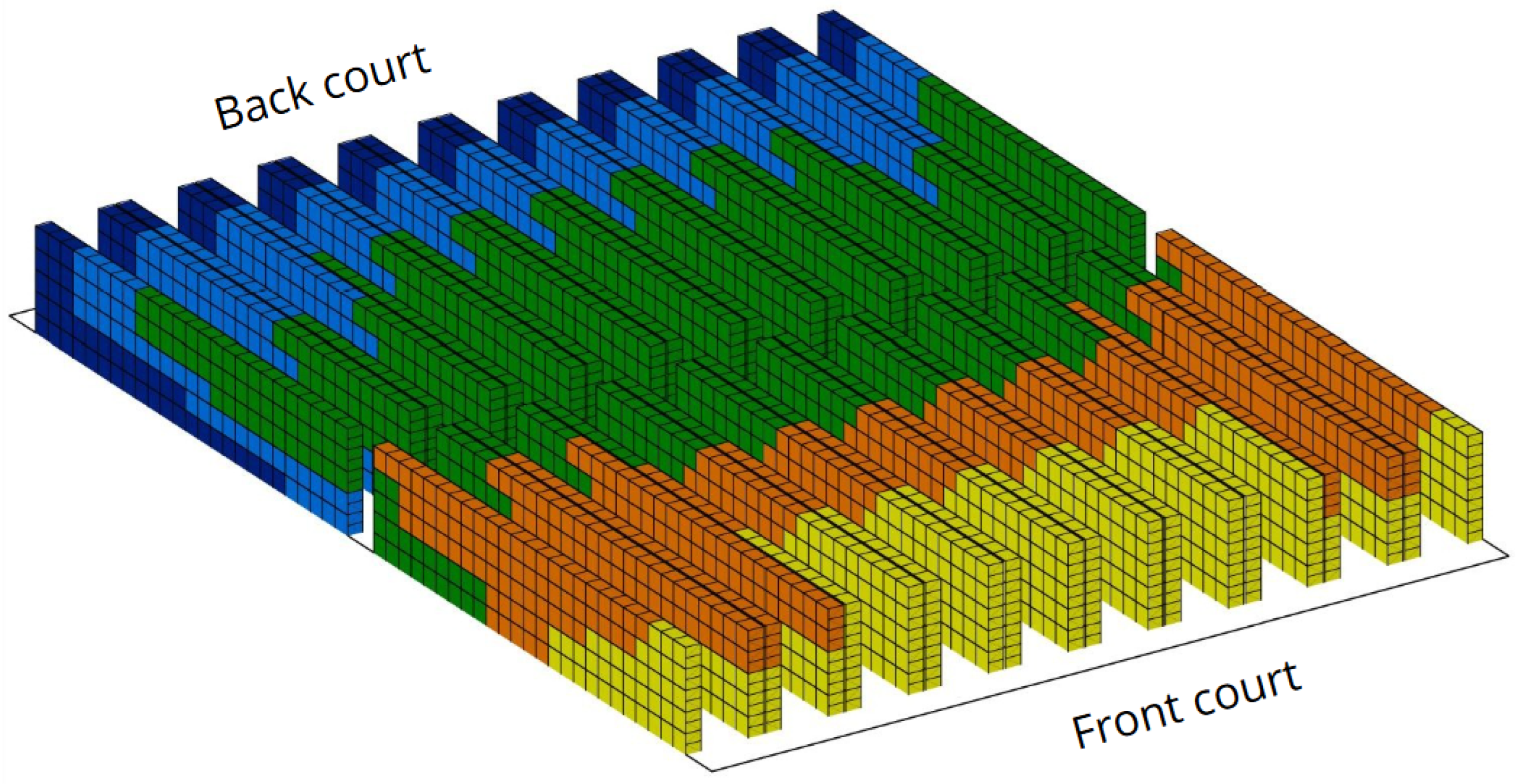
Figure 3.
Comparison of the average storage cycle time for approach and in scenario S1.
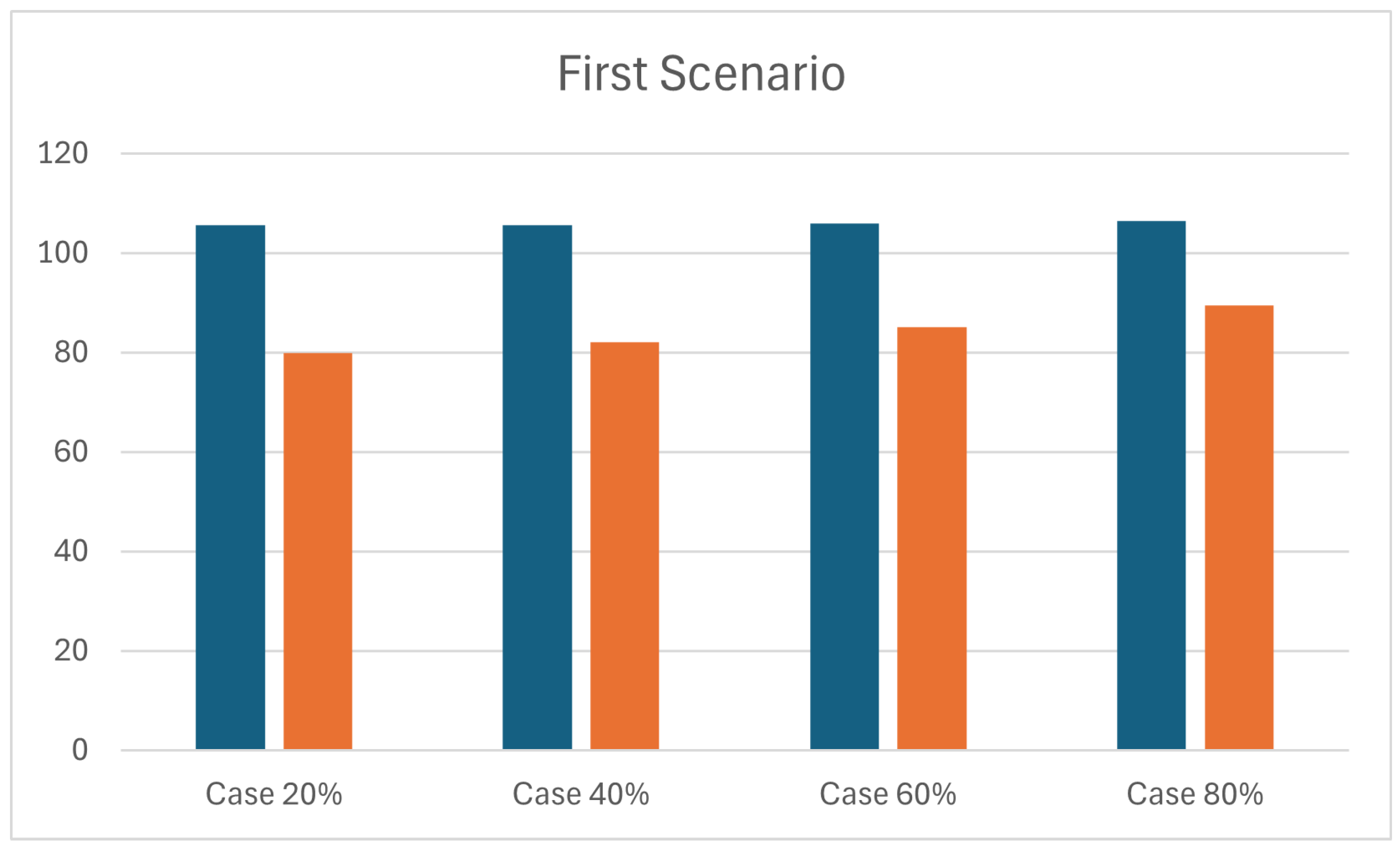
Figure 4.
Top view of the barycentre of the case 20% (red point represent case , black point case ).
Figure 4.
Top view of the barycentre of the case 20% (red point represent case , black point case ).
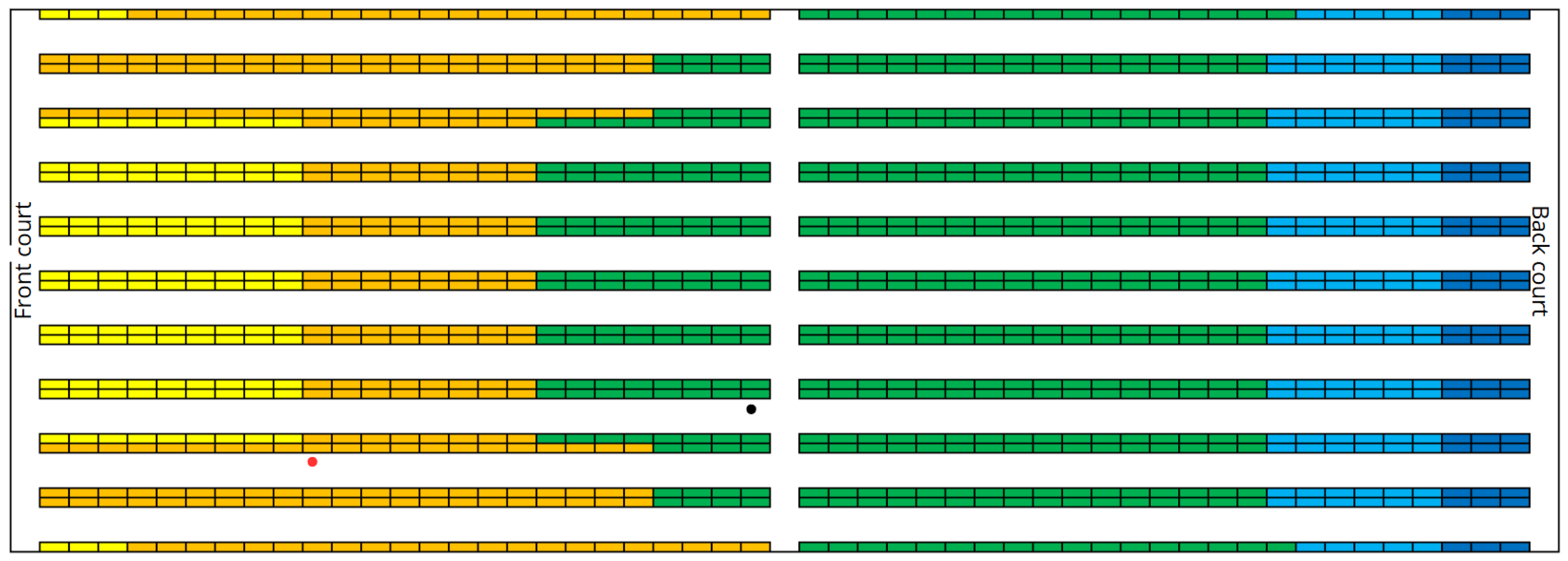
Figure 5.
Top view of the barycentre of the case 40% (red point represent case , black point case ).
Figure 5.
Top view of the barycentre of the case 40% (red point represent case , black point case ).
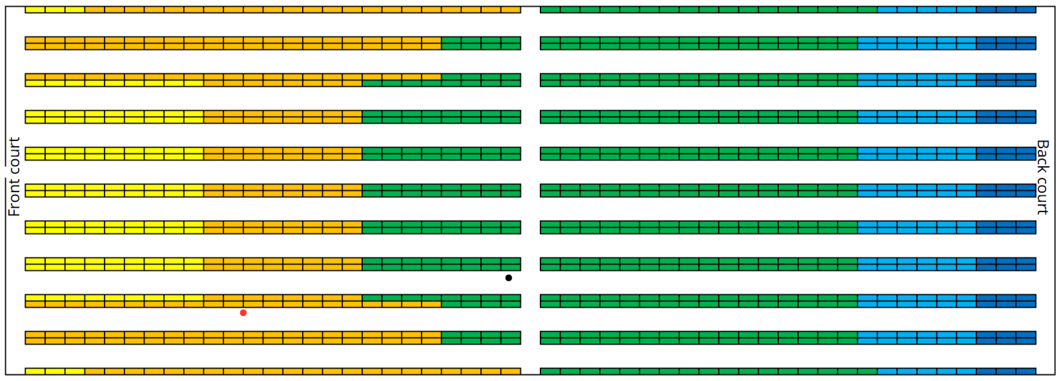
Figure 6.
Top view of the barycentre of the case 60% (blue point represent case , black point case ).
Figure 6.
Top view of the barycentre of the case 60% (blue point represent case , black point case ).
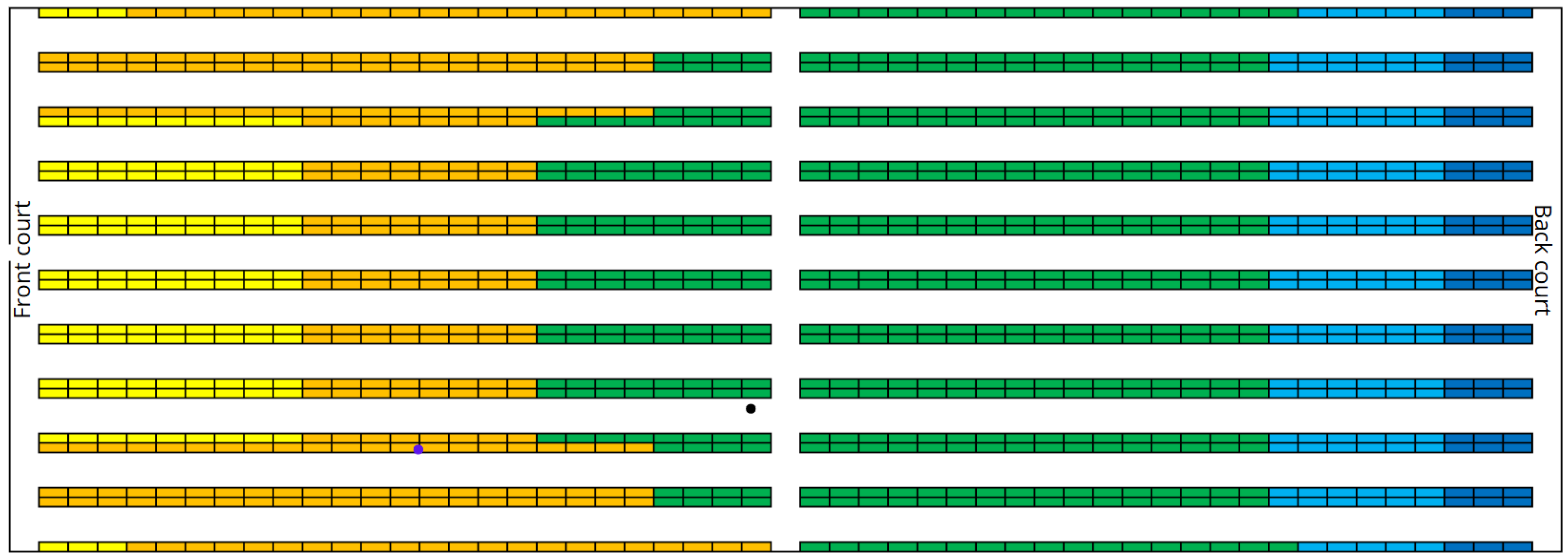
Figure 7.
Top view of the barycentre of the case 80% (blue point represent case , black point case ).
Figure 7.
Top view of the barycentre of the case 80% (blue point represent case , black point case ).
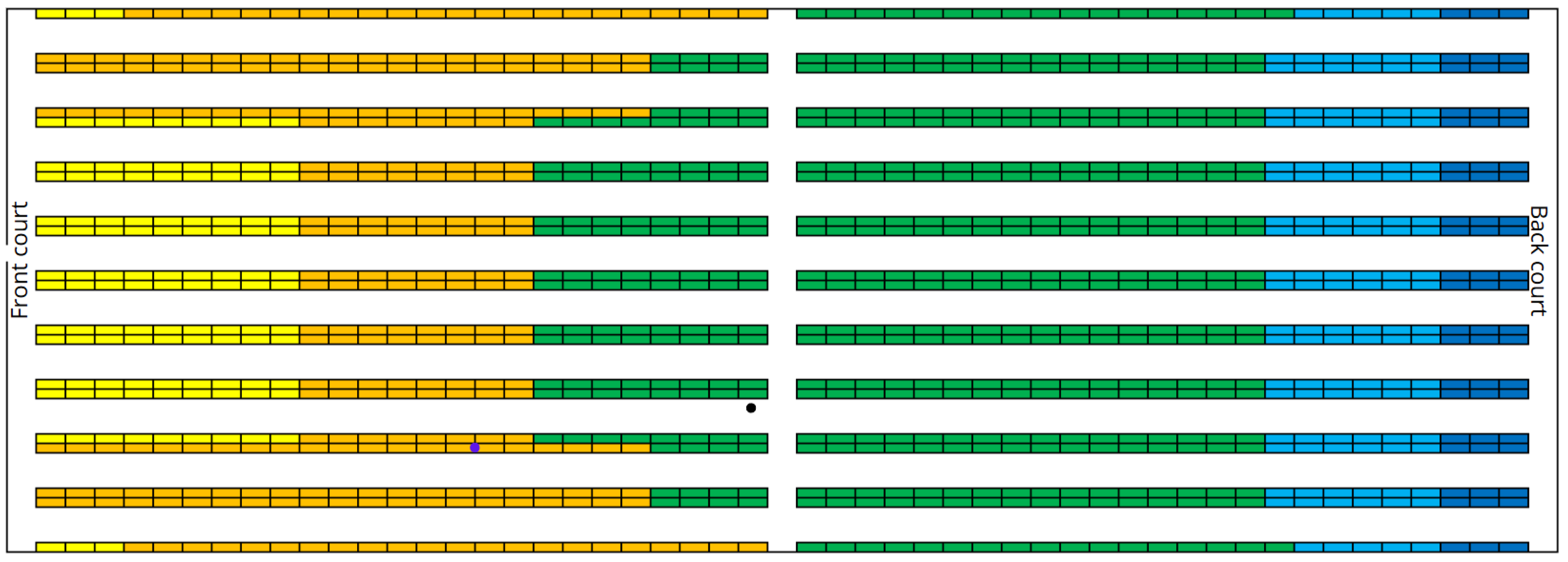
Figure 8.
Comparison of the average storage cycle time for approach and in scenario S2.
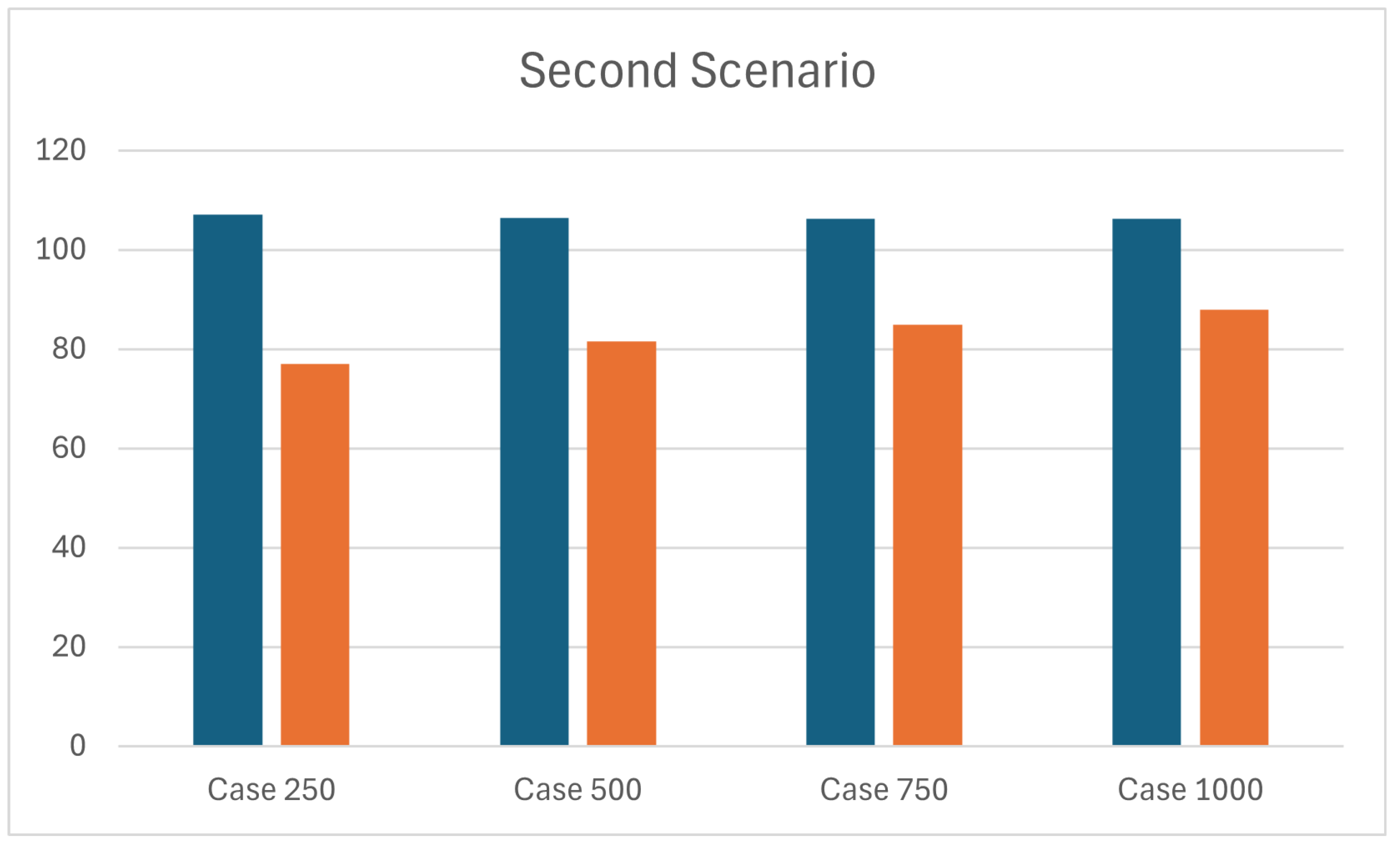
Figure 9.
Comparison of the average storage cycle time for approach and in scenario S3.
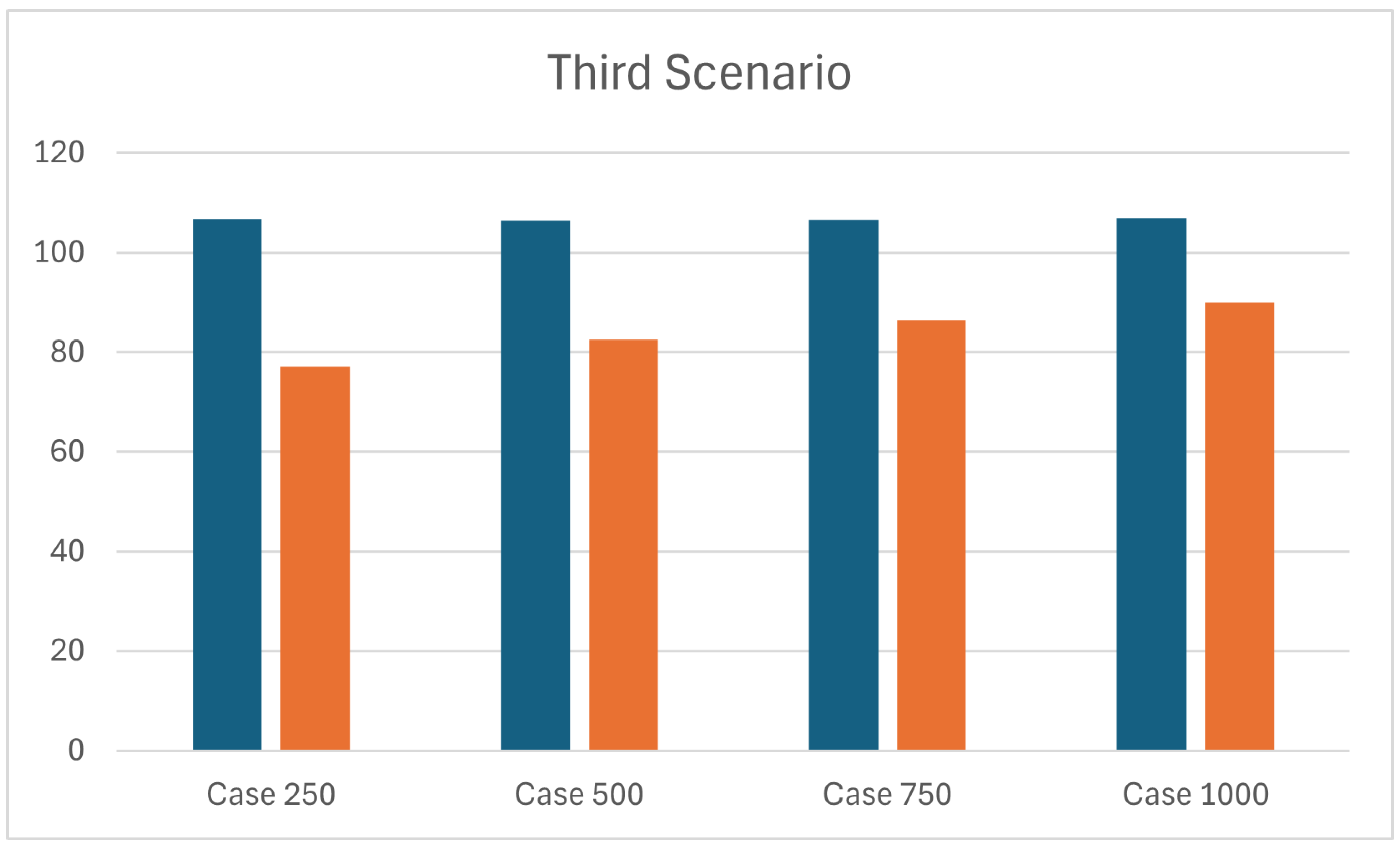

Table 1.
Parameters related to warehouse layout and forklift operations.
| Parameter | Description | Value |
|---|---|---|
| Width of the aisles along x-axis | 2 m | |
| Width of the aisles along y-axis | 4 m | |
| Length of each unit load | 1.2 m | |
| Width of each unit load | 0.8 m | |
| h | Height for each storage level | 1.5 m |
| c | Clearance distance within each load | 0.075 m |
| Travel speed of an empty forklift truck | 3.5 m/s | |
| Travel speed of a loaded forklift truck | 3 m/s | |
| Unloaded fork ascending speed | 0.5 m/s | |
| Loaded fork ascending speed | 0.3 m/s | |
| Unloaded fork descending speed | 0.5 m/s | |
| Loaded fork descending speed | 0.5 m/s | |
| Pallet forking and deforking time | 60 s |
Table 2.
Values of for each sub-case within scenario S1 and for approaches and .
| Case | () | () |
|---|---|---|
| [seconds] | [seconds] | |
| 20% | 105.595 | 79.898 |
| 40% | 105.665 | 82.148 |
| 60% | 105.971 | 85.129 |
| 80% | 106.426 | 89.466 |
Table 3.
Coordinates of barycentre for each sub-case within scenario S1 and for approaches and .
| Case | () | () |
|---|---|---|
| [metres] | [metres] | |
| 20% | (33.485, 13.805, 3.060) | (14.751, 10.652, 0.782) |
| 40% | (33.704, 14.071, 3.017) | (16.491, 10.975, 0.965) |
| 60% | (33.427, 14.430, 3.065) | (18.663, 11.261, 1.238) |
| 80% | (34.263, 14.412, 3.055) | (21.726, 11.979, 1.613) |
Table 4.
Values of for each sub-case within scenario S2 and for approaches and .
| Case | () | () |
|---|---|---|
| [seconds] | [seconds] | |
| 250 | 107.088 | 77.034 |
| 500 | 106.431 | 81.434 |
| 750 | 106.249 | 84.917 |
| 1000 | 106.157 | 87.840 |
Table 5.
Coordinates of barycentre for each sub-case within scenario S2 and for approaches and .
| Case | () | () |
|---|---|---|
| [metres] | [metres] | |
| 250 | (34.530, 13.983, 3.198) | (12.977, 9.319, 0.606) |
| 500 | (34.632, 13.413, 3.129) | (16.271, 10.730, 0.885) |
| 750 | (34.317, 14.530, 3.002) | (18.114, 11.539, 1.230) |
| 1000 | (34.655, 14.435, 2.957) | (20.611, 11.775, 1.461) |
Table 6.
Values of for each sub-case within scenario S3 and for approaches and .
| Case | () | () |
|---|---|---|
| [seconds] | [seconds] | |
| 250 | 106.790 | 77.074 |
| 500 | 106.373 | 82.503 |
| 750 | 106.558 | 86.462 |
| 1000 | 106.920 | 89.851 |
Table 7.
Coordinates of barycentre for each sub-case within scenario S3 and for approaches and .
| Case | () | () |
|---|---|---|
| [metres] | [metres] | |
| 250 | (33.214, 14.457, 3.240) | (12.803, 9.713, 0.588) |
| 500 | (33.770, 14.467, 3.096) | (16.136, 10.273, 1.038) |
| 750 | (34.589, 14.843, 2.992) | (18.998, 11.756, 1.392) |
| 1000 | (34.757, 14.674, 3.060) | (21.751, 12.008, 1.679) |
Disclaimer/Publisher’s Note: The statements, opinions and data contained in all publications are solely those of the individual author(s) and contributor(s) and not of MDPI and/or the editor(s). MDPI and/or the editor(s) disclaim responsibility for any injury to people or property resulting from any ideas, methods, instructions or products referred to in the content. |
© 2025 by the authors. Licensee MDPI, Basel, Switzerland. This article is an open access article distributed under the terms and conditions of the Creative Commons Attribution (CC BY) license (http://creativecommons.org/licenses/by/4.0/).
Copyright: This open access article is published under a Creative Commons CC BY 4.0 license, which permit the free download, distribution, and reuse, provided that the author and preprint are cited in any reuse.


