Submitted:
25 July 2025
Posted:
25 July 2025
You are already at the latest version
Abstract
This paper proposes a methodology for the generation and registration of three-dimensional data sets to support an adaption of teach and repeat path following for an Autonomous Underwater Vehicle (AUV) equipped with a multibeam sonar. The goal of this system is to enable an AUV to generate a topological map of a path consisting of locally consistent sub maps and to re-follow this path using newly collected data. For AUVs traversing long distances without external navigational aids, this methodology would allow robust return-to-home capability, specifically in remote and harsh environments such as beneath ice.
Keywords:
AUV
; navigation
; multibeam
; teach and repeat
; visual navigation
1. Introduction
General navigation of an underwater robot is a challenging problem due to the limitations of providing an external positioning source [1,2]. This problem becomes greater for robots that wish to travel tens to hundreds of kilometres in uncharted and uncertain regions, such as those areas beneath floating ice at the polar regions of the earth. In this context, robots such as Autonomous Underwater Vehicles (AUVs) may be required to rely solely on their onboard sensors and computers to maintain sufficient knowledge of where they are and how they should proceed to complete their defined task and ultimately return to a location that allows safe recovery.
The traditional approach to this problem is the use of onboard attitude and heading sensors combined with a velocity sensor, generally a bottom tracking Doppler Velocity Log (DVL) [3,4]. The attitude, heading, and velocity are combined to perform dead-reckoning, where a known starting position is periodically propagated along the sensed vector of travel through integration.
In the absence of any other motion, the position of the AUV in the global North-East coordinate system , with North-relative heading , and body referenced velocities of in the forward and starboard direction respectively, can be updated by the following equations:
With an initial estimate of and repeated integration of measured velocities, and heading, , the position of the AUV can be estimated at any time.
The measured heading and velocities are imperfect, suffering from both measurement noise and systematic biases [3,5]. Over time these measurements are integrated, the propagated position will deteriorate, and the estimate will not reflect the true location. For the work presented here, the International Submarine Engineering (ISE) Explorer AUV is used. The vehicle utilises an iXBlue PHINS INS [6] and a Teledyne Workhorse DVL. In optimal conditions the rated positional accuracy is of the distance travelled by the AUV. This rate is under ideal conditions, however higher rates have been observed in the field [4]. This performance is typical for a survey grade AUV, but can be much worse for smaller, cheaper platforms.
DVLs work by projecting sound energy towards the seafloor and analysing the returned signal, specifically the Doppler shift which it equates to the relative velocity of the AUV to the seafloor. Depending on the power and frequency of the sensor, there is a minimum and maximum range from the AUV from which the velocity can be measured. In addition, excessive rotational motion of the AUV (i.e. pitch and roll) can limit returns from the seafloor. In instances where the seafloor cannot be accurately referenced for velocity, the DVL may provide a velocity reference to the water column itself or no reference at all. The former introduces the influence of water currents, where returned velocities are no longer relative to the fixed seafloor but relative to the motion in the ocean. The latter presents periods where no measured velocity is available and the navigation must rely solely on inertial measurements and exponentially increasing errors.
1.1. Problem Statement
Given the potential for a degrading global navigation estimate, an AUV may be in a situation where returning to a home location is risky or unlikely. This is more pronounced when operating in a narrow corridor on very long paths and in the presence of a degraded sensor. This ability to safely return to a home location once a primary task has been achieved, or abandoned, is the primary motivation for this work. Specifically in the context of exploration beneath floating ice shelves, where returning along the path taken may be the most likely, or only, safe path back to a safe recovery. This problem space is discussed in more detail by the author here [7,8]. Within this context, the focus is purely on the ability to reliably retrace a path and not to improve our estimate of global position.
The driving force of this work is to enable a robust and reliable ability to follow a path previously traversed in the presence of imperfect sensors, with no reliance on an estimate of global position. This work was motivated by the need to improve the reliability of AUVs operating in the Antarctic by improving their ability to return to a safe recovery location and was developed using data collected in the field near the Thwaites Glacier.
2. Background and Related Work
This work builds on prior work in the field of geophysical based navigation where a sensor is utilised to detect and classify some aspect of the environment to generate some informative updates to the navigation [3,9]. Specifically, the sensor considered in this work is a multibeam sonar given its popularity of use on AUVs. This work can be considered part of the author’s larger body of work described here [2,8,10], which describes the problem statement and proposed solution utilising sonar images generated from a side-scan sonar. Much of the background theory is the same with the methodology altered to utilise a different class of sensor.
Geophysical navigation most generally attempts to associate a present set of measurements of the environment with some prior collected data of an overlapping area. This can be an entire map of the region of operations provided prior to the deployment, such as in [11,12], or data collected earlier in the same deployment. For the latter a classification is made based on whether the map is collected in a distinct mapping phase, or if the mapping and data association occur concurrently. The latter is termed Simultaneous Localisation and Mapping (SLAM) and many works are available on the topic [3,9,13,14]. It is the former which relates most closely to our problem statement, where a reference map is collected during an initial phase, then utilised on a return phase. The most common description of this type of approach is Teach and Repeat [15,16,17], with some references to Sequential Visual Homing [18,19].
2.1. Teach and Repeat Path Following
The foundations for Teach and Repeat (TR) path following are based on the fact that a robot with imperfect sensing capabilities will generate imperfect maps. These maps will be globally inconsistent, but for navigation to occur they need only be locally consistent to enable robot autonomy [20]. As discussed earlier in this section, our ability to maintain an estimate of our position deteriorates over time, but over a short span of time our estimates are satisfactory. The errors will divert us from the global truth, but over a short time scale our estimates will agree locally.
The key concept in TR navigation is that the map of the environment is represented as a connected set of these locally consistent spaces, or views [21]. These connections are logical, such as nodes on a graph, to avoid establishing erroneous metric relationships beyond the capability of our sensing methods [22]. Locally sensed data will be consistent and show coherence with prior views of the same region. For navigation throughout the space a logical approach of associating the next view in the path is relied upon. The navigation then becomes a matter of steering the vehicle towards the next node, not explicitly driving it to a location.
Achieving the target location in the path is a process of localising to a node through sensing and directing the vehicle along a sequence of nodes that arrive at the goal. The solution becomes more akin to homing the vehicle towards the goal, rather than strict navigation. Functioning TR systems have been successfully demonstrated by the work of Furgale and Barfoot [15] in which a robot rover traversed a repeat path over 32km and by the author’s own work, where TR methodologies were adapted and tested on an AUV in [2] utilising a sidescan sonar.
The primary difference in this work and previous works is the adaption to an underwater vehicle utilising a downward facing multibeam. The AUV is floating in its medium and thus has six-degrees of freedom, the sensor is fixed to the AUV, and the seafloor remains fixed. The views are constructed not as images, but as three-dimensional tiles that accurately represent the seafloor. This context is what distinguishes the methods presented here.
3. Methodology
3.1. Conventions
The conventions are based on the SNAME conventions for submerged bodies [23] and are used when referencing the pose and position of the AUV, the global inertial frame, and the data coming from the multibeam sensor.
The global frame and any estimates therein are defined as an inverted right-hand rule, labelled the North-East-Down (NED) frame with the axes N extending positive to North, E positive to East, and Z extending positive downward. Heading is rotation about the vertical axis, represented as and positive during rotation from North to East. For this work positions are in metres assuming a local horizontal flat plane representation of the earth, in line with the local Universal Transverse Mercator (UTM) zone. Where translation is required from this reference to an ellipsoid representation, the World Geodetic System (WGS) 84 is assumed.
We define a body-frame fixed to a reference point on the AUV. The axis defined as x, extending along the longitudinal axis of the AUV with velocity u, positive towards the bow or nose. The y axis extends along the transverse axis, with velocity v, positive towards starboard. The z axis is orthogonal to x and y, and positive down. We define roll (p) as rotation about the , positive when the port side rises, pitch (q) as rotation about the y axis, positive as the nose rises, and Yaw (r) as rotation about z, positive as the nose moves towards starboard. Measurements are discrete with an associated time. We do not consider linear acceleration or angular velocity in our calculations.
3.2. Multibeam Sonar
This work utilises three-dimensional multibeam sonar data collected along the seafloor below the AUV as it travels along its prescribed route. The multibeam sonar periodically transmits an acoustic pulse and utilizes the received echo to generate an array of relative range vectors. These vectors are regularly spaced along an arc producing a horizontal swath along the sensor’s transverse axis. The angular component of these vectors is relative to the sensor’s centre and the magnitude is the slant range distance from the sonar head to the estimated point of contact with the seafloor as illustrated in Figure 2.
Each ping returns an array of ranges and a corresponding array of angles of length n, where n is the number of beams per ping. In this work, n and A are fixed values for the entirety of a mission.
The multibeam sonar is rigidly mounted to the AUV, and thus, the range vector arrays are fixed relative to the AUV body frame of reference. As the AUV travels along its path, sequential arrays of sonar data are combined to generate a three-dimensional representation of the seafloor which should remain consistent over time such that if the AUV were to cover the same area again, the representations would be coherent.
An AUV includes sensors that measure its motion and attitude relative to the world around it. This is required for navigation. In its most basic form, an AUV will measure its speed, heading, and orientation within the global frame. From the AUV navigational information we can take each array of bathymetric range samples and determine where each point lies on the seafloor, such that a local map of seafloor measurements can be constructed and referenced on subsequent visits. The process involves translating the sonar relative vectors to the body reference frame, then to earth-relative locations.
3.3. Pose Merging
Each individual ping of multibeam data is recorded and timestamped on an onboard computer at some fixed ping rate. Concurrently, the vehicle’s pose, or position and attitude, is estimated by the INS and the data is logged to the AUV main computer and timestamped, generally at a higher rate. Individual computers are kept relatively time-synced through a common Network Time Protocol (NTP) server. Prior to applying corrections from the INS data to the multibeam, the individual data records are first aligned by time. To align the data, each multibeam ping is assigned to the nearest navigation record in time, within an expected tolerance of one-half the INS sampling period. This ensures that each multibeam record has navigation information that is within one half of the INS recording period.
In this work, the Pandas Python library is utilised to manage each dataset as a DataFrame object. For the merging, the provided merge_asof function takes the two datasets, indexed by time, and systematically merges them by finding the nearest match within the provided tolerance. The field data used in this work has multibeam data collected at approximately 1.5Hz, and navigation data at 10Hz. We utilise a tolerance of . Upon merging we get an average time difference between the multibeam record and the INS data of 0.025s, with a standard deviation of 0.016. As our AUV platform is relatively slow moving at 2.0m/s and generally stable in yaw and pitch, as shown in Figure 3, we do not perform any interpolation.
This merged dataset contains timestamped records of all required information to cast the sensor samples into a representation of the covered seafloor. The AUV’s onboard estimate of position is not utilised in this process as the primary motivation of this work is to generate an independent estimate of position, free from accumulated error.
The relative positions are generated from measured speed and heading, which when integrated over a short time scale suffer less error growth stemming from sensor noise and bias. For example, a well behaved navigation system with DVL bottom lock will exhibit and error rate of 0.001 of distance travelled [6]. If our tiles are merely 100m long, then we’d only expect a localised error across the tile of 0.1m. In the worse case of no seafloor speed reference, we could expect 3m of error [6]. This error would remain relatively constant per tile, no matter how long the mission.
3.4. 3D Point Set Generation
From the merged dataset we apply the necessary corrections to take the individual sonar-relative range vectors and project them into a local earth-relative NED-frame. These steps vary depending on a particular sensor and vehicle, so the following are based on the configuration of our AUV at the time of the field data collection, but the principles and techniques are generally applicable.
Each multibeam record holds an array of raw slant range and relative angle. The raw ranges are based on the time of travel of the sound pulse from the sensor head to the seafloor and back using a fixed estimate of sound speed in water of . Therefore, each raw range is corrected using the current AUV measured sound velocity:
Where is the adjusted array of range values at time t and the measured speed of sound.
The range and angle vectors are converted into an array of points in the AUV body-frame using basic trigonometric transformations and offsets from the sonar centre to the body-frame centre as follows:
Filtering is then applied to remove points that are considered invalid. As the points are now relative to the AUV body-frame, we utilise the AUV’s own measure of seafloor range, or altitude, to remove points that do not fall within some reasonable tolerance. The AUV altitude is taken from the DVL and is an average of 4 beams projected down and away from the vehicle. The measured altitude is very resistant to noise. The multibeam provides raw range samples and it is not uncommon for a portion of the samples to be invalid. An assumption is made that each valid multibeam z-value should be within of the measured altitude. For this work, altitudes are in the range of 75 meters from the seafloor, thus allowing points that vary 37.5 meters, which in terms of expected seafloor morphology is ample. This will eliminate many noisy outlier points but generates many false-positives. This is done at the present stage to reduce the number of points requiring further calculation. This is summarised below in Equation 5.
where is the DVL measured height above seafloor.
To place the AUV relative points into the local NED-frame we apply in order the measured roll, pitch, and yaw and add the measured AUV depth below sealevel to the resultant z component, as shown in Equation 6.
3.5. Local Map Generation
To create a local map multiple sequential arrays of earth-corrected points, , are combined using the relative motion of the AUV between each point array to place them topographically in a point set, as depicted in Figure 4. For instance, if the AUV was moving forward along the North axis, the arrays would be aligned along the direction of travel, with their N coordinate spaced by the distance travelled between each sample instance.
Formally, from an initial ping we determine the relative displacement for each subsequent ping in the plane based on speed of travel, heading, and the elapsed time. The N and E components of the displacement are then added to the vector resulting in a set of points projected to the local seafloor, as shown in Equation 7 and visually in Figure 4. The number of pings included in each tile segment is pre-selected.
3.6. Filtering
As the points are relative to their true seafloor representation, the fact that the seafloor is a continuous surface is used to further reduce any residual noise in the data. The Z value should of each sample should be consistent with the points nearest to it, and those that are inconsistent are likely erroneous. For each point in our set we look at those points closest in the dimensions and compare the point’s Z value to the general mean and variance of its neighbours. If it agrees with the local distribution it is kept, if it does not it is removed. We limit our search to a maximum distance away from the point and to a maximum number of neighbours to improve efficiency. The filter threshold is some number of standard deviations above and below the mean.
To facilitate a fast comparison of each point to those around it we organise our point data into a KD_Tree. This balanced tree structure, where each node is a point in the set, allows efficient searches for neighbouring points. In this work we utilise the SciPy implementation cKDTree [24]. Performance is expected to be for building the tree, and for search, where n is the number of points in the tile.
The final result is a set of points, or point cloud. The set of all point clouds forms the input to the navigation system described in subsequent sections.
3.7. Data Preparation Workflow
The complete workflow of preparing the raw data for the path-following system is shown systematically in Figure 5.
4. Teach and Repeat Implementation
This work is foundational to an eventual implementation of a TR path following system for an AUV with mounted multibeam sonar. Thus, all further analysis will be in the context of application to a TR system. Utilising work as described in Section 2.1 the core concepts of TR are applied to this particular work. Fundamentally the system operates in two distinct phases. First, a teach phase is enabled while the AUV performs some initial task, in our case an exploratory mission into an unknown environment where the AUV must return to its point of departure upon task completion, or failure, to ensure safe recovery. The AUV collects a sequential set of local sub-maps along the travelled path, internally organising them as a directed graph where each vector is a map tile and the edges are the logical connections to the next node in the path. The nodes are aware of their relative position to the path start based on the AUV navigation and the relative vector to the subsequent node. Figure 6 illustrates this logical association of data with a reference set.
The second phase is a repeat phase triggered either by task completion or by some detected condition that warrants abandonment of the path goal. These conditions are more fully described in [8]. During this phase, as the AUV collects new tile-maps, they are compared to the stored reference map of tiles and localisation is attempted. With sufficient belief that our position along the map is known, we utilise the relative node-to-node vectors to steer the AUV such that it achieves each node in sequence to complete a return to the path origin.
The steps and data flow for each phase are shown visually in Figure 7.
4.1. Tile Association
A key functionality in all geographic or terrain-relative navigation schemes is the ability to reliably compare data collected in some area and determine the likelihood that it represents an area for which prior data exists. In this work, a set of points representing a recently collected tile is compared to the set of existing reference tiles to determine how likely it matches.
We can consider the set of reference tiles and the candidate tile to be two measurements of the same entity - the three-dimensional shape of the seafloor. Coincident measurements should be similar with some associated noise. From related works a common approach is to model this comparison as Gaussian [25] where the likelihood is a measurement of probability that the difference between the measurements is zero. The probability density function of this likelihood is represented as a Gaussian function:
Where x is the measured value, is the mean, or expected value, and the standard deviation.
Given a candidate tile consisting of a set of depth measurements Z at locations , we extract a set of potential locations from the reference map. Drawing on work in Iterative Closest Point (ICP) registration [26], for each location in the candidate set we find the closest point in the reference set, within some tolerance, to perform the likelihood calculation. Similar to work in [25], our likelihood calculation utilises the mean square of the difference between point sets, given as:
Where is the subset of measurement points with an associated point from the reference set, denoted , and are the corresponding standard deviations, and n the number of corresponding nearest point pairs. The use of a subset of the measurement set is purely to reduce computational load, and the amount of sub-sampling is explored as a parameter in our analysis of the control test results below.
4.2. State Estimation
The goal of the state estimation is to reliably and repeatedly determine the most likely pose of the AUV relative to the reference path using newly acquired sensed data, in this case a bathymetry tile. Each tile is a view of a potential location along the reference map, changing with each update as the AUV moves. This is an example of robot localisation, one of the most essential problems in robotics [27], and one of the most studied.
The state locations belong to the set of two-dimensional coordinates covered by the map. The state changes between observations are determined by the motion of the AUV, and are not necessarily linear, nor are they perfectly measurable. The platform’s instantaneous motion is affected by the forces acting upon it, such as buoyancy, current, thrust, hydrodynamic reaction, and its control surfaces. The overall path is determined by the navigational algorithms which set the target waypoints and make decisions regarding the final executed path, which though deterministic, are dynamic and responsive to the environment.
During each update cycle we consider a newly acquired tile against all possible locations in the state space to determine a measure of likelihood that a particular location best represents the location of the AUV, should one exist. If there is a sufficiently likely location we then consider this our estimate of location, or more formally, the current state.
In implementing a TR system, we consider a couple of caveats to inform our decision on the selection of a state estimator. First, we consider the path to be a set of discrete nodes along a logical path, where each node has a position and a reference to the relative location of the next node. Second, at any time we must consider that we have no idea where our AUV is starting its return path journey, so we begin in a state of total entropy; known as global localisation. Third, we must consider that the AUV may fall off the path due to unforeseen factors, such as environmental, vehicle dynamics, or conflicting mission task, and thus even if our path position is known, we may lose our place and must return to the initial state of total entropy; a scenario referred to as the kidnapped robot problem [28,29].
Considering finite locations and the need for global localisation, our problem is not merely a tracking problem. With feature-based TR as described in [2] the system only has to consider an estimate of the most likely node, and the path offset is inferred by the feature matching itself. The utilisation of 3D points gives only the likelihood of location, with no implied offset, thus offset positions must be included in the state space. Therefore, a fixed histogram/grid-based approach may not be tractable. For example, a 30km path would result in approximately 100 nodes and thus require many 1000s of possible states to account for the multitude of offsets.
To limit the search for the most likely estimate of state we instead utilise a particle filter (PF), an implementation of a non-parametric Bayesian estimator that uses a finite set of estimates distributed throughout the state space instead of a complete set of estimates. This is similar to the approach taken in [12]. The locations of each estimate, or particle, evolves as updates arrive and the belief in the most likely estimate represented by the distribution of locations of all the particles.
We initiate the filter as a set of randomly chosen state estimations evenly distributed across the state space. For our application this is a set of n positions within the coverage area of the reference map. The choice of n influences the computation load of the system as each particle requires a likelihood calculation, but also the ability of the filter to represent the belief as more particles can better cover the search space and can better represent the true distribution of belief.
Formally our particle locations X can be described as n randomly chosen positions from the set of all positions included in the reference set :
Following initialisation the filter operates on a sequence of predict-update steps triggered as each new tile is received. The prediction uses the measured motion process of the AUV to first re-project each particle to a new location. The update step then calculates the likelihood of each particle. The resultant value assigned as the importance, or weight, of that particle. The resultant weighted distribution at any step represents the posterior belief of the filter.
On its own this filter will suffer from degeneracy as a few particles will quickly gain most of the distribution weight, i.e. those nearest the true state, leaving the majority of particles with little to no influence on the estimate, but still consuming computational resources. To overcome this the particle set is subject to re-sampling, where particles are selected based on their normalised weight. This re-sampling utilises replacement, such that particles with high relative weights may be selected multiple times, and low-weight particles not at all. The weights of this new set is re-initialised and the distribution of particles over the state-space in the new set reflects the belief distribution.
Again there is a risk that strong particles will continue to dominate, as those with high relative weights will be selected more often, leading to many copies of the same particle, known as impoverishment [30,31]. To combat this, during the update step we consider the fact that our prediction is based on measured motion and is not perfect, there is an element of uncertainty. As each particle is updated we introduce an element of random process noise to each particle. This effectively causes identical particles to spread out and diversify. Impoverishment can be avoided with sufficient process noise, and we also directly introduce additional noise through roughening, or jitter [30,32]. The amount of jitter introduces is a key parameters explored in the analysis of our control test results below.
5. Trials and Results
5.1. General
The methodologies described in this work were tested on data collected in-field from the primary area of interest, beneath the ice in Antarctica. Testing focused on validating the system’s ability to generate a reference set from raw sensor data and reliably register and localise using updated raw sensor data. Though testing was strictly offline, the methods utilised would be compatible with an online implementation. The onboard capabilities of TR are demonstrated in [2].
5.2. Data Collection
Data for this work was collected during a deployment of the University of Tasmania’s ISE [30] built Explorer AUV, nupiri muka, to the Thwaites Glacier region of Western Antarctica [8]. The missions conducted by the AUV represent the exact use-case for the developed TR system and saw the AUV conduct a long-range incursion beneath the ice to achieve a set target location toward the grounding line, followed by a planned return along the same track.
Deployment was from the Korean research ice-breaker Araon, which held station at the launch and recovery site. Given the range of the missions and the ice cover, there was no ability to provide external acoustic tracking or positioning, so the AUV relied solely on its ability to maintain a deck-reckoned estimate of its position.
Figure 8 shows the area of operations and the mission track used in this work. Multibeam data was collected during the incursion and return missions. The planned path was such that there is a high degree of overlap between incursion and return data. Figure 9 shows the sensor coverage for both the outward and return.
Missions were run at a fixed altitude from the seafloor of and speed set-point of . The multibeam was an Imagenex 837B Delta-T [31] configured to collect 120 samples across a 120o swath at a rate of . AUV navigation data was collected at .
5.3. Tests
The mission data was split into the in-run and the out-run sections. TR tests were conducted using two cases: control tests in which the in-run and out-run datasets are each used as both the teach and repeat run; trial test in which each data set is used as teach with the other as repeat. The control cases allow analysis of key parameters in an idealised situation where the repeat data matches the reference data exactly. The trial tests are true performance tests of the expected ability of the TR system operating on real-data where the two data sets are non-coincident.
We evaluate the performance of each test by looking at our knowledge of where the most likely location match should be, based on the onboard navigation. Though we do not utilise this navigation in the TR system, it is useful for evaluation. During our control tests, we expected that our estimated position at any given time would match the onboard position, within some distribution due to the likelihood calculation. At each step along the path following algorithm we calculate the estimated position, which is the average position of all particles, the tile position as reported by the AUV, and the nearest associated reference path location for both the estimate and the reported location.
5.4. Likelihood Performance
Using the control tests we analyse the ability of the likelihood function alone to discern tiles that should match compared to those that should not. A tile is selected from the path and compared to itself and the set of neighbouring tiles both preceding and following based on path index. We expect the likelihood to be highest when compared to itself versus its neighbours. The resultant likelihoods are normalised to allow relative comparison over multiple test sets. Figure 10 shows the results of tiles compared against their 40 closest neighbours. In all cases the self-comparison, or 0-offset case, resulted in the highest relative likelihood.
Beyond tile-to-tile comparison, the likelihood function should also discern the most valid positional offset. Again considering the control case where a tile is compared against itself over a set of offsets from 0 in all directions should provide insight. Figure 11 illustrates the result of computing the likelihood of a tile against itself for a range of two-dimensional offsets. As expected the likelihood is maximised as we approach an offset of 0.
In regard to parameters, only the sub-sampling affects the likelihood calculation. It has an affect on execution time, as with increased sub-sampling fewer points are being compared. Results shown in Figure 12 indicate a reduction in execution time, but with diminishing returns beyond a factor of 10.
Availing of reduced computation should not come at the expense of functionality. Figure 13 illustrates that even up to a factor of 100, there is no discernible impact on likelihood performance.
5.5. Control Results
For the control tests three core criteria were considered: 1) How many update steps did it take the system to arrive at a confident estimate of position; 2) Did the system maintain a correct estimate for the duration of the run; and 3) How well did the estimated relative positions match the AUV INS positions. To help tune the system, the performance is considered across the key parameters discussed in Section 4: the amount of sub-sampling used in the likelihood calculation, the number of particles in the filter, and the amount of process noise jitter.
For criteria 3 we take the distance from the TR system’s estimate to the recorded AUV INS position, referred to as the error. A summary of the results from the control runs is shown in Table 2 for a given set of parameter choices.
Figure 14 shows the error results for three selected control runs based on the return path data set. These plots visualize the evolution of the system as each update step progresses. As expected there is an initial stage of maximum uncertainty that converges and maintains over the remainder of the test.
In all cases the system was able to gain and maintain an estimate of the AUV’s position within 3-5 update cycles. In regard to the number of particles we can observe the main effect in the distribution of overall error across the runs, as shown in Figure 15. Generally, we see an improvement in the error with a higher number of particles, as expected. In the case of 5000 particles the majority of results are within a band of 3-6m.
For jitter we see an improved performance with higher jitter, more pronounced with less particles. This is intuitive as more particles can better represent the distribution naturally, but fewer particles would benefit from increased diversity through jitter. In the cases of 500 and 1000 particles, jitter improves error performance across the board, but for 5000 particles the effect is less obvious.
As indicated in the analysis of the likelihood function, the use of sub-sampling has no clear effect on performance of the state estimation, other than to reduce computation load.
5.6. Trial Results
For the test results we have two distinct datasets collected at different times with variations in their actual trajectory and environmental influences, such as tides and currents. These tests are an accurate measure of the system’s ability to function in a real-world scenario as the data was collected in the exact fashion as would occur in a real-world deployment. Again we consider the same criteria as in the control tests, but with the knowledge that the estimated and INS positions will never agree exactly, as the two runs are afflicted by the inherent errors discussed earlier in the paper. For this analysis the error is only indicative as during the trials there was no true measure of the navigation error.
Table 3 is a summary of the results against relevant parameters of particle set size and jitter. We utilised a fixed sub-sampling of 10 based on prior analysis. Again we see that in all cases the system maintained a correct estimate of the path tile location once global initialisation completed.
Figure 16 shows the distribution of error over all tests, with the majority of mean error, once localised, within a band of 20-50m. If we consider the path length was 30km and the AUV was purely dead-reckoning this error band is within our expected of distance travelled.
Figure 17a shows results for a single out-run as reference and return-run as repeat, and return-run as reference, and Figure 17b the inverse. We see an initial phase of global localisation where the error reduces with each update and then maintains itself within a band of less than 20m. Given the overall length of the runs and the temporal separation, this is well within an acceptable range of error across the runs.
Collection of data in the target area is a massively expensive undertaking in regard to time, money, and the logistics required. The test data utilised in this work represents months of planning and many weeks of operating in one of the most remote regions on Earth. So though the quantity of test data was limited, it is a true indication that the proposed methodology can work in this environment under real operating conditions. The results are truly encouraging and have value for future exploration.
6. Discussion
The results are very promising, showing that a tile-based localisation methodology will work with AUV collected multibeam data. The determination of likelihood between each new tile and the reference set provided a sufficient belief factor to allow the particle filter first obtain and then maintain an estimate of location along the path that closely matched the true location. The number of particles used in the filter affected the overall gross error, where more particles tended to provide a better result, but at the cost of increased need for processing resources. The particle set sizes selected for test results, 1000 and 5000, provide a good balance of performance and efficiency and would be suitable for on-board deployment on the target hardware. Where processing time is less that the time needed to generate a new tile.
Over the set of tests conducted, the system was able to successfully gain and maintain an estimate of relative position to the reference path, within an error value consistent to the expected navigation error of the AUV. If we consider that the primary test data was taken from a 30km mission track, and an idealised performance metric of dead-reckoning, we would expect an error accumulation of 30m along each of the mission transects. From Figure 15 we can see that the majority of residual error for the 5000 particle case was approximately 5m, and 10m for the 1000 particle case. From Figure 16 we see a true performance of 20m for the 5000 particle case and 25m for the 1000 particle case. The improvements become more relevant when we consider that any real deployment would not be idealised and additional navigational errors would be present due to any deep-diving periods where DVL seafloor referencing was unavailable, and in periods of dynamic terrain where the DVL may drop out.
For real world missions, the improvements of this methodology are clear, and improve as we perform longer missions.
7. Conclusions and Future Work
This work presented a methodology for using a multibeam sonar on an AUV in an adaption of Teach and Repeat (TR) path following. This type of system has important application to long-range deployment of AUVs in difficult environments, such as beneath ice, where navigation along an already traversed path is important. This work shows that a TR system is feasible for use in our target environment and was tested using actual data collected by the candidate platform in Antarctica. We believe this is the first such demonstration of a TR based system utilising a multibeam sonar.
As an adaption to other work utilising sidescan sonar discussed in [2], the inclusion of multibeam data will extend the utility of a TR based system for more general use on AUVs. This is most evident for AUVs equipped with only multibeam, such as those performing terrain mapping. For AUVs that have both sidescan and multibeam capability there are cases where one system is preferred to the other. Firstly, multibeam can generally operates at farther ranges from the seafloor, thus allowing the AUV to maintain more separation from the bottom in areas of dynamic terrain. Secondly, the physical characteristics of the seafloor may favour one system to another. A flat seafloor with sediment based features would work well with sidescan, but less so with multibeam, whereas an area with consistent sediment by distinct slopes the inverse.
Though testing was limited, it was conducted on real data under real conditions. Future work would require in-field testing of the system in a controlled environment, as in [2].
References
- M. V. Jakuba, C. N. Roman, H. Singh, C. Murphy, C. Kunz, C. Willis, T. Sato, R. A. Sohn, Long-baseline acoustic navigation for under-ice autonomous underwater vehicle operations, Journal of Field Robotics 25 (11-12) (2008) 861–879. [CrossRef]
- P. King, A. Vardy, A. L. Forrest, Teach-and-repeat path following for an autonomous underwater vehicle, Journal of Field Robotics 35 (5) (2018) 748–763. [CrossRef]
- L. Paull, S. Saeedi, M. Seto, H. Li, Auv navigation and localization: A review, IEEE Journal of Oceanic Engineering 39 (1) (2014) 131–149. [CrossRef]
- R. McEwen, H. Thomas, D. Weber, F. Psota, Performance of an auv navigation system at arctic latitudes, IEEE Journal of Oceanic Engineering 30 (2) (2005) 443–454. [CrossRef]
- A. Tal, I. Klein, R. Katz, Inertial navigation system/doppler velocity log (ins) fusion with partial dvl measurements, Sensors 17 (2) (2017) 415.
- Phins surface (Dec 2022). https://www.ixblue.com/store/phins-surface/.
- P. King, G. Williams, R. Coleman, K. Zürcher, I. Bowden-Floyd, A. Ronan, C. Kaminski, J.-M. Laframboise, S. McPhail, J. Wilkinson, A. Bowen, P. Dutrieux, N. Bose, A. Wahlin, J. Andersson, P. Boxall, M. Sherlock, T. Maki, Deploying an auv beneath the sørsdal ice shelf: Recommendations from an expert-panel workshop, in: 2018 IEEE/OES Autonomous Underwater Vehicle Workshop (AUV), 2018, pp. 1–6. [CrossRef]
- P. King, K. Zürcher, I. Bowden-Floyd, A risk-averse approach to mission planning: nupiri muka at the thwaites glacier, in: 2020 IEEE/OES Autonomous Underwater Vehicles Symposium (AUV), 2020, pp. 1–5. [CrossRef]
- F. Maurelli, S. Krupiński, X. Xiang, Y. Petillot, Auv localisation: a review of passive and active techniques, International Journal of Intelligent Robotics and Applications (2021) 1–24.
- P. King, B. Anstey, A. Vardy, Sonar image registration for localization of an underwater vehicle, The Journal of Ocean Technology 12 (3) (2017) 68–90.
- G. Salavasidis, A. Munafò, C. A. Harris, T. Prampart, R. Templeton, M. Smart, D. T. Roper, M. Pebody, S. D. McPhail, E. Rogers, et al., Terrain-aided navigation for long-endurance and deep-rated autonomous underwater vehicles, Journal of Field Robotics 36 (2) (2019) 447–474.
- B. Claus, R. Bachmayer, Terrain-aided navigation for an underwater glider, Journal of Field Robotics 32 (7) (2015) 935–951. [CrossRef]
- S. B. Williams, O. Pizarro, M. V. Jakuba, I. Mahon, S. D. Ling, C. R. Johnson, Repeated auv surveying of urchin barrens in north eastern tasmania, in: 2010 IEEE International Conference on Robotics and Automation, 2010, pp. 293–299. [CrossRef]
- I. Mahon, S. B. Williams, O. Pizarro, M. Johnson-Roberson, Efficient view-based slam using visual loop closures, IEEE Transactions on Robotics 24 (5) (2008) 1002–1014.
- P. Furgale, T. D. Barfoot, Visual teach and repeat for long-range rover autonomy, Journal of field robotics 27 (5) (2010) 534–560. [CrossRef]
- T. Krajník, F. Majer, L. Halodová, T. Vintr, Navigation without localisation: reliable teach and repeat based on the convergence theorem, in: 2018 IEEE/RSJ International Conference on Intelligent Robots and Systems (IROS), 2018, pp. 1657–1664. [CrossRef]
- T. Nguyen, G. K. Mann, R. G. Gosine, A. Vardy, Appearance-based visual-teach-and-repeat navigation technique for micro aerial vehicle, Journal of Intelligent & Robotic Systems 84 (2016) 217–240. [CrossRef]
- R. Möller, A. Vardy, Local visual homing by matched-filter descent in image distances, Biological cybernetics 95 (5) (2006) 413–430. [CrossRef]
- M. Liu, C. Pradalier, F. Pomerleau, R. Siegwart, Scale-only visual homing from an omnidirectional camera, in: 2012 IEEE International Conference on Robotics and Automation, IEEE, 2012, pp. 3944–3949.
- R. Brooks, Visual map making for a mobile robot, in: Proceedings. 1985 IEEE International Conference on Robotics and Automation, Vol. 2, IEEE, 1985, pp. 824–829.
- Y. Matsumoto, M. Inaba, H. Inoue, Visual navigation using view-sequenced route representation, in: Proceedings of IEEE International conference on Robotics and Automation, Vol. 1, IEEE, 1996, pp. 83–88.
- S. Simhon, G. Dudek, A global topological map formed by local metric maps, in: Proceedings. 1998 IEEE/RSJ International Conference on Intelligent Robots and Systems. Innovations in Theory, Practice and Applications (Cat. No.98CH36190), Vol. 3, 1998, pp. 1708–1714 vol.3. [CrossRef]
- Nomenclature for treating the motion of a submerged body through a fluid, The Society of Naval Architects and Marine Engineers, Technical and Research Bulletin (1950) (1950) 1–5.
- P. Virtanen, R. Gommers, T. E. Oliphant, M. Haberland, T. Reddy, D. Cournapeau, E. Burovski, P. Peterson, W. Weckesser, J. Bright, S. J. van der Walt, M. Brett, J. Wilson, K. J. Millman, N. Mayorov, A. R. J. Nelson, E. Jones, R. Kern, E. Larson, C. J. Carey, İ. Polat, Y. Feng, E. W. Moore, J. VanderPlas, D. Laxalde, J. Perktold, R. Cimrman, I. Henriksen, E. A. Quintero, C. R. Harris, A. M. Archibald, A. H. Ribeiro, F. Pedregosa, P. van Mulbregt, SciPy 1.0 Contributors, SciPy 1.0: Fundamental Algorithms for Scientific Computing in Python, Nature Methods 17 (2020) 261–272. [CrossRef]
- S. Barkby, S. Williams, O. Pizarro, M. Jakuba, An efficient approach to bathymetric slam, in: 2009 IEEE/RSJ International Conference on Intelligent Robots and Systems, 2009, pp. 219–224. [CrossRef]
- Z. Zhang, Iterative point matching for registration of free-form curves and surfaces, International journal of computer vision 13 (2) (1994) 119–152. [CrossRef]
- S. Thrun, W. Burgard, D. Fox, Probabilistic Robotics (Intelligent Robotics and Autonomous Agents), The MIT Press, 2005.
- S. P. Engelson, D. V. McDermott, Error correction in mobile robot map learning, in: Proceedings 1992 IEEE International Conference on Robotics and Automation, IEEE Computer Society, 1992, pp. 2555–2556.
- H. Choset, K. Lynch, S. Hutchinson, G. Kantor, W. Burgard, L. Kavraki, S. Thrun, Principles of robot motion: Theory, algorithms, and implementation errata!!!! (2007).
- Explorer auv (Feb 2018). https://ise.bc.ca/product/explorer/.
- Imagenex, 837B Delta T 6000 m Profiling, revised May 2017 (2023).
Figure 1.
(a) Body frame of reference. (b)Global frame of reference.
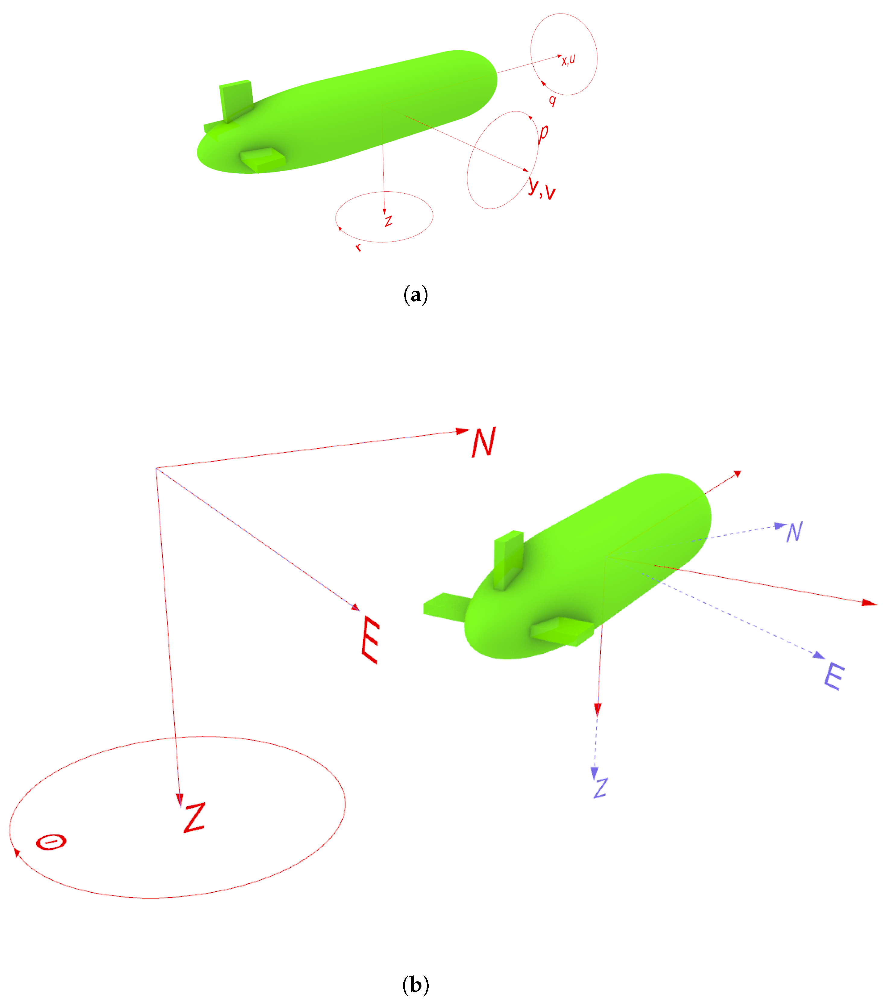
Figure 2.
Multibeam vectors. Each consist of an angle relative to the sensor’s vertical axis and the measured range from the sensor to the point of contact on the seafloor.
Figure 2.
Multibeam vectors. Each consist of an angle relative to the sensor’s vertical axis and the measured range from the sensor to the point of contact on the seafloor.
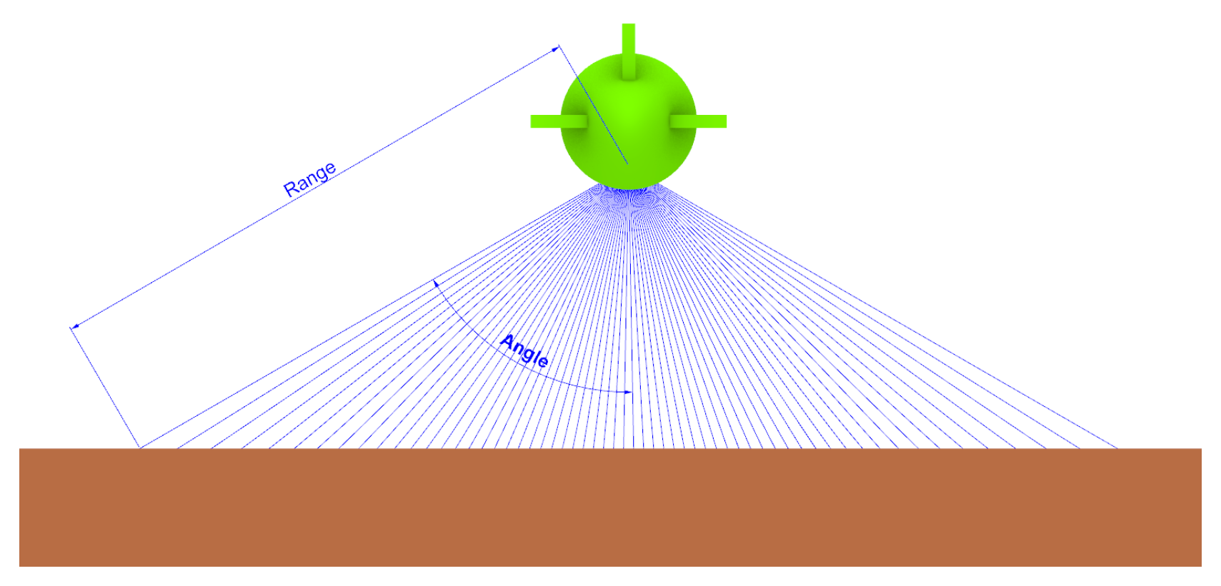
Figure 3.
Histogram of AUV rotations to show the general stability of the Explorer AUV. Mean values are: Yaw 0.04, Pitch 0.1, Roll 0.1.
Figure 3.
Histogram of AUV rotations to show the general stability of the Explorer AUV. Mean values are: Yaw 0.04, Pitch 0.1, Roll 0.1.
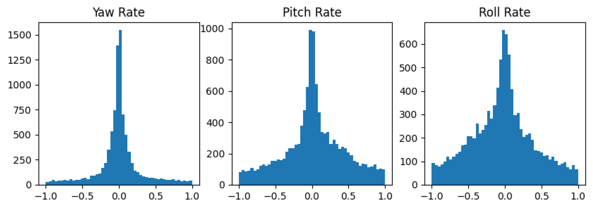
Figure 4.
Tile point data projected into the global frame based on AUV depth, orientation.
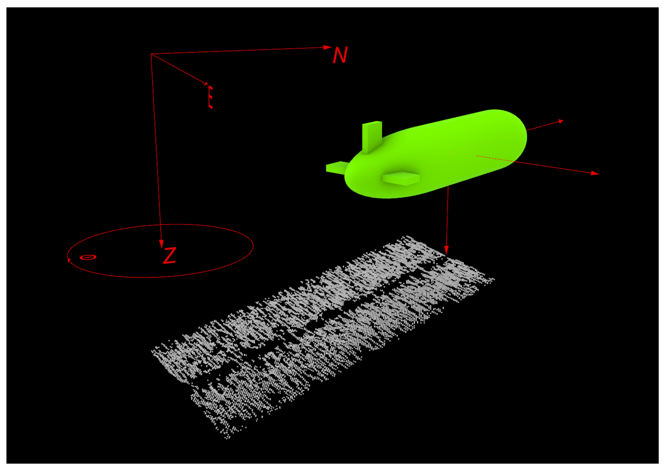
Figure 5.
Data preparation and tile generation.
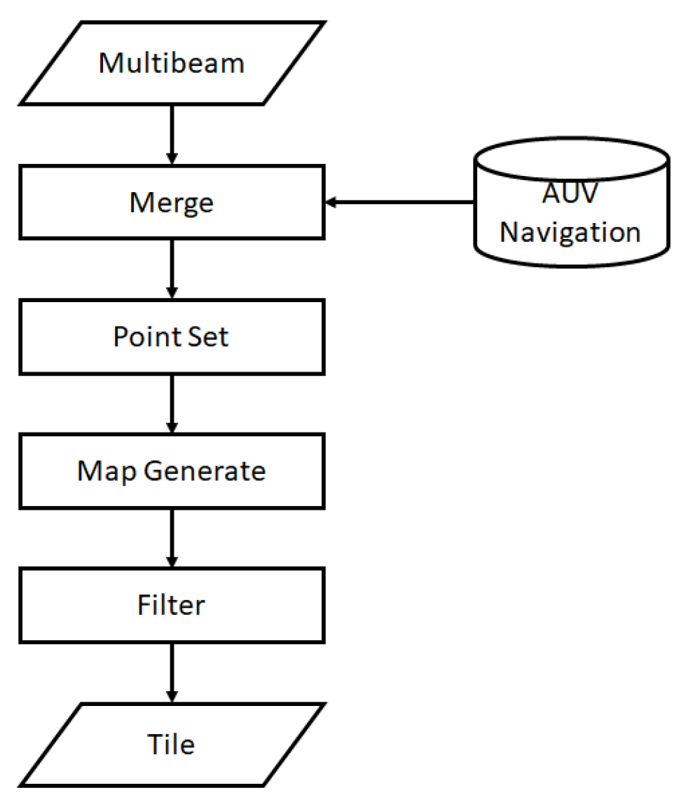
Figure 6.
TOP: Raw multibeam data coloured by depth. MIDDLE: Multibeam data coloured by its index in the reference path. BOTTOM: Tile metadata for a particular tile.
Figure 6.
TOP: Raw multibeam data coloured by depth. MIDDLE: Multibeam data coloured by its index in the reference path. BOTTOM: Tile metadata for a particular tile.
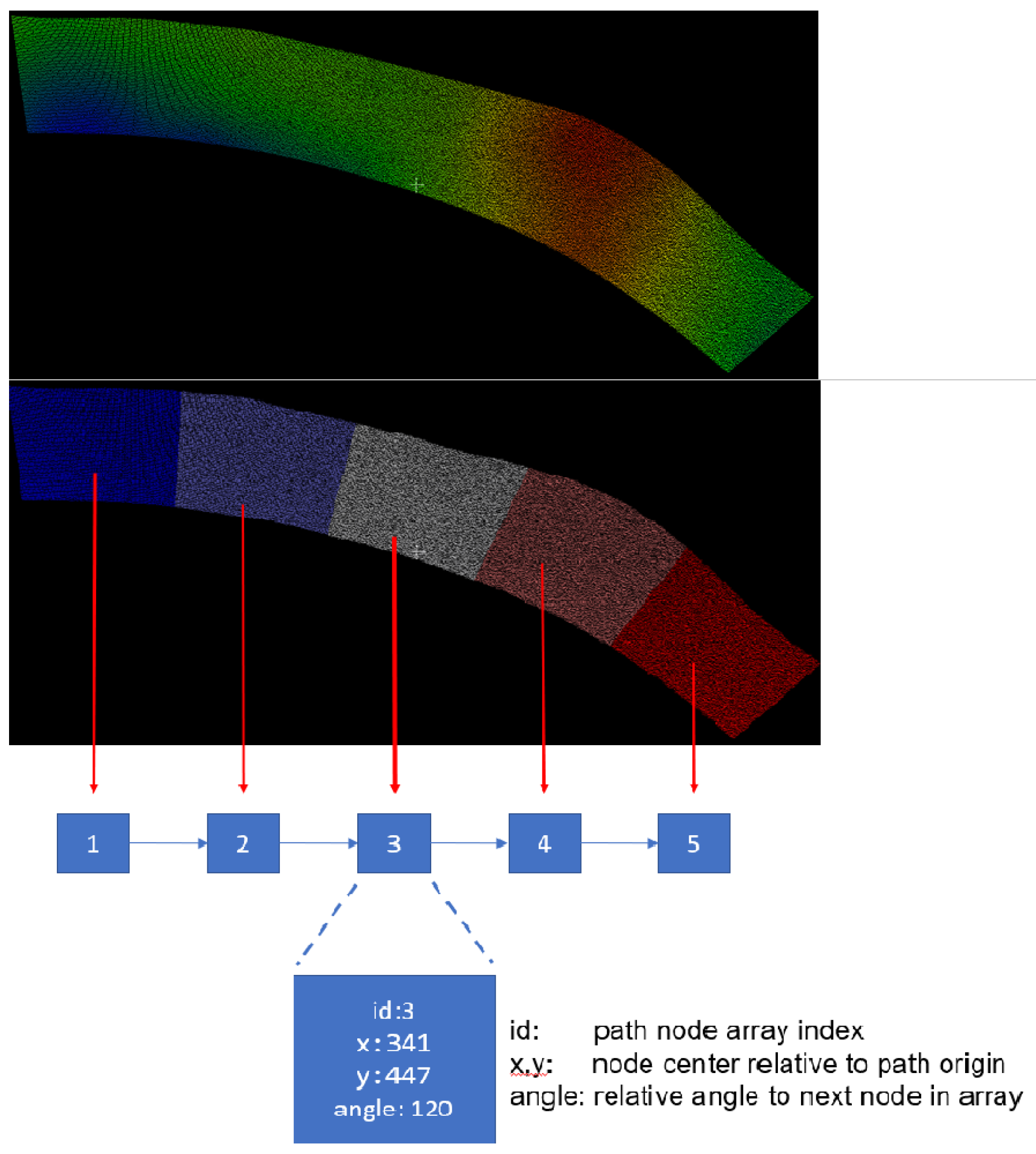
Figure 7.
Flowcharts for: (a) Teach phase, (b) Repeat phase.
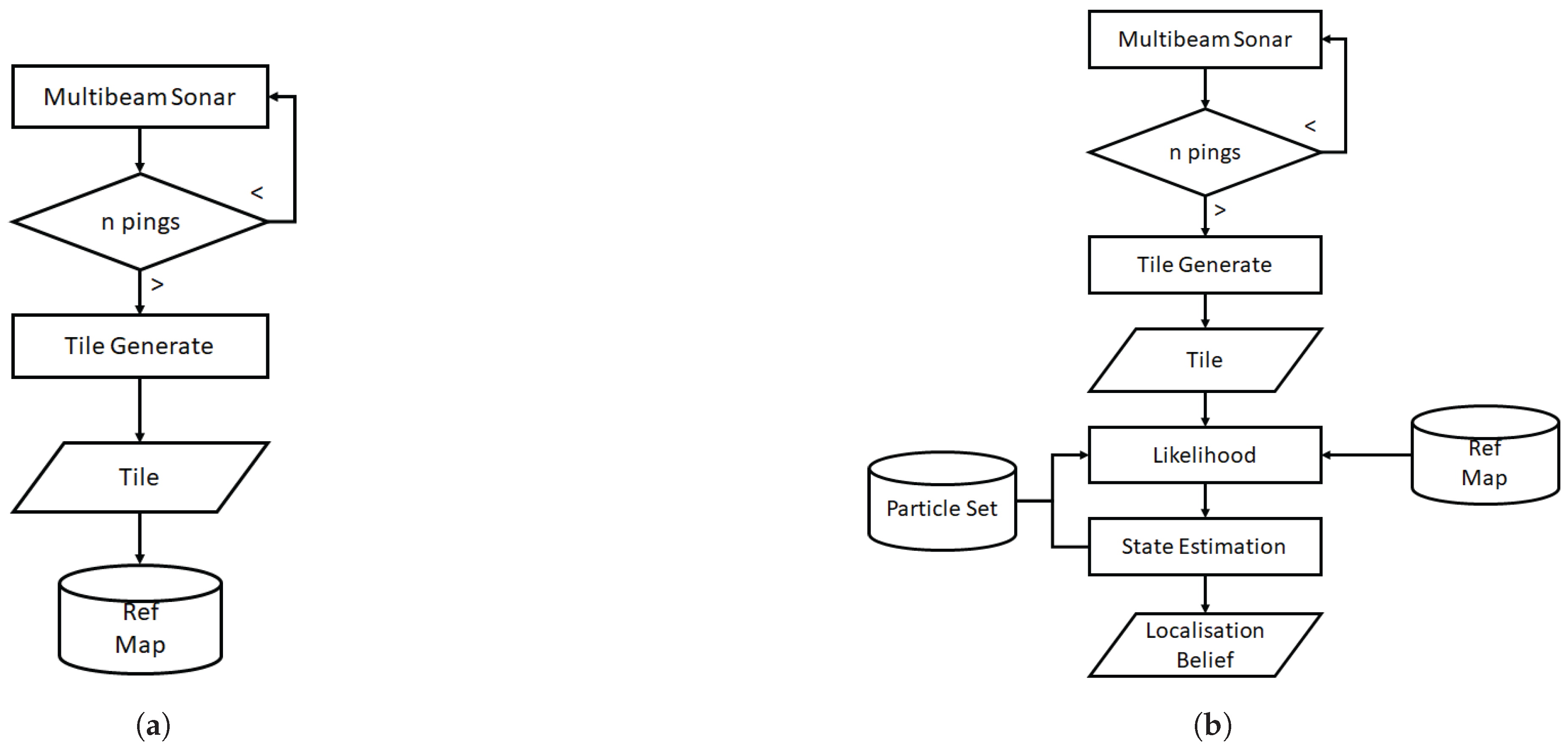
Figure 8.
Executed mission track from nupiri muka deployment to Thwaites Glacier 2020. Mission m6_30km (yellow) is the primary dataset used in this work.
Figure 8.
Executed mission track from nupiri muka deployment to Thwaites Glacier 2020. Mission m6_30km (yellow) is the primary dataset used in this work.
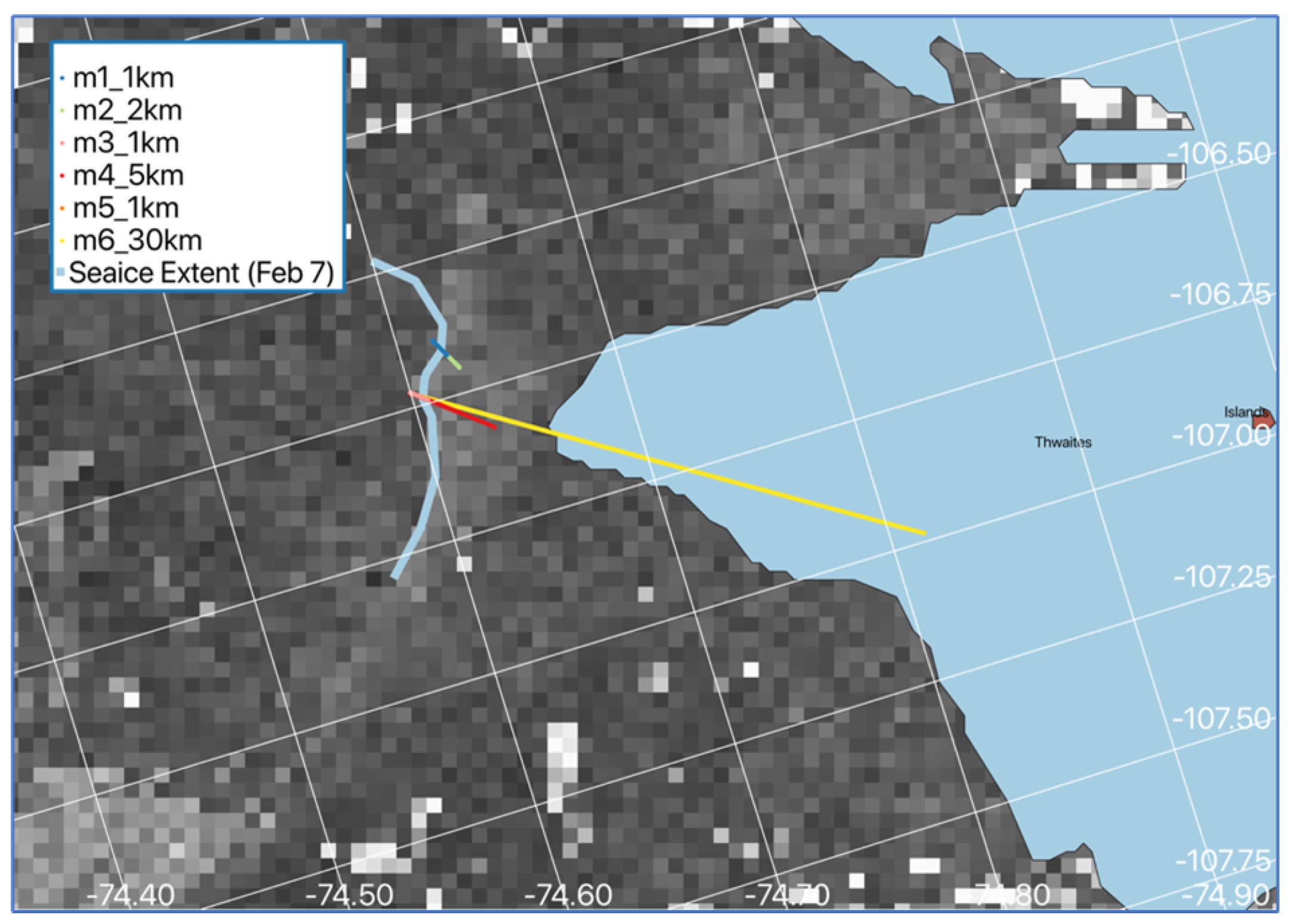
Figure 9.
Lines used for testing. Green is the inward path, Red the outward return path.
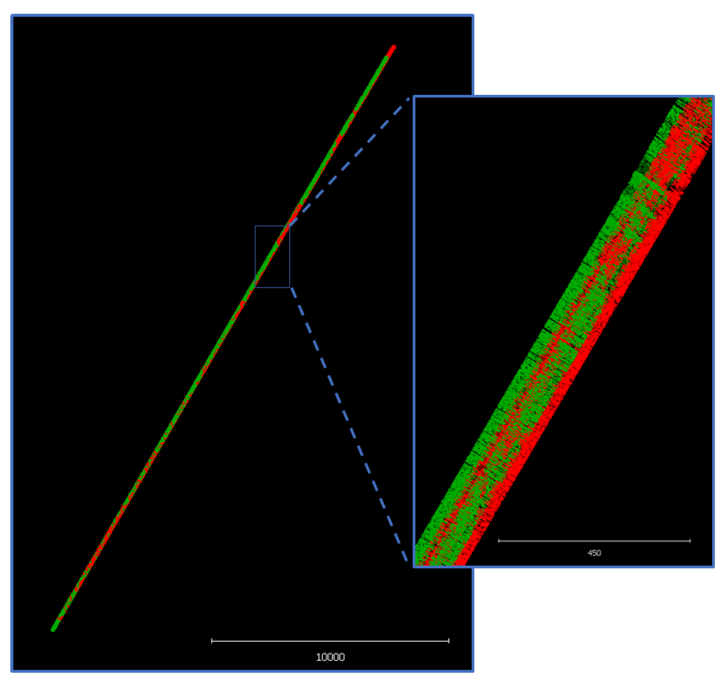
Figure 10.
Normalised likelihood of tiles compared against neighbouring tiles proceeding and following by path index.
Figure 10.
Normalised likelihood of tiles compared against neighbouring tiles proceeding and following by path index.
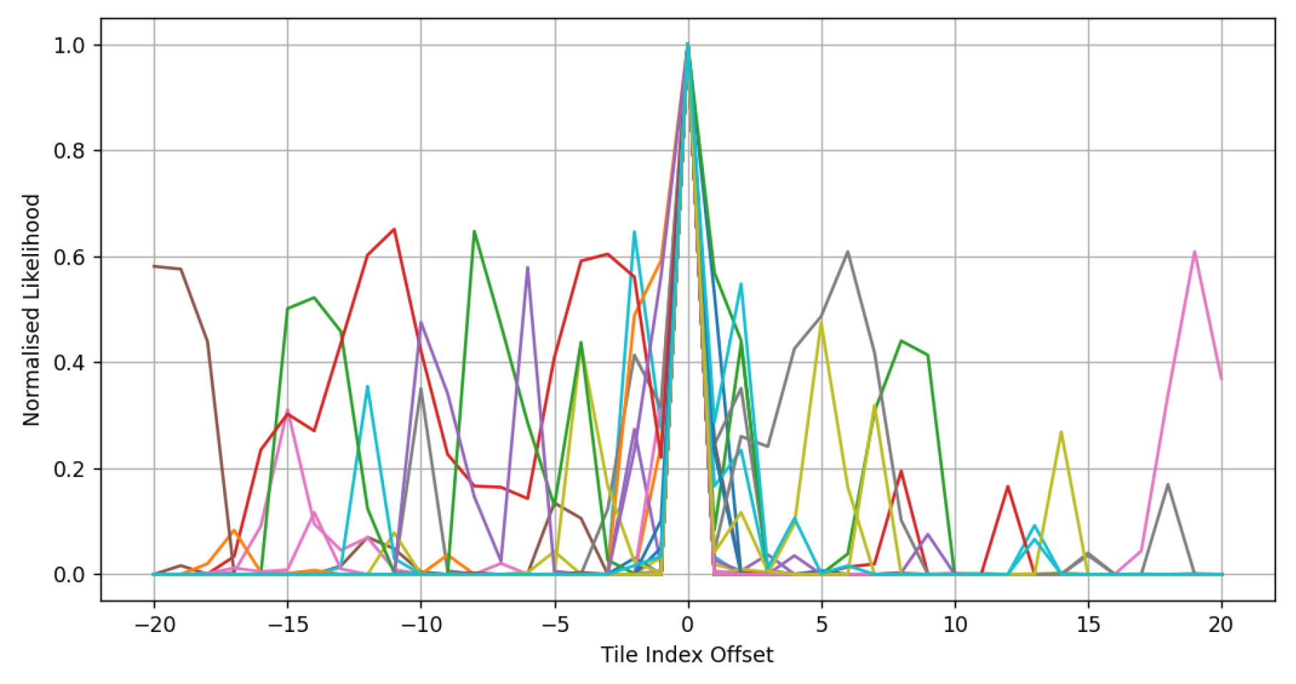
Figure 11.
Likelihood as calculated over a series of two-dimensional offsets. Both colour and size are proportional to likelihood.
Figure 11.
Likelihood as calculated over a series of two-dimensional offsets. Both colour and size are proportional to likelihood.
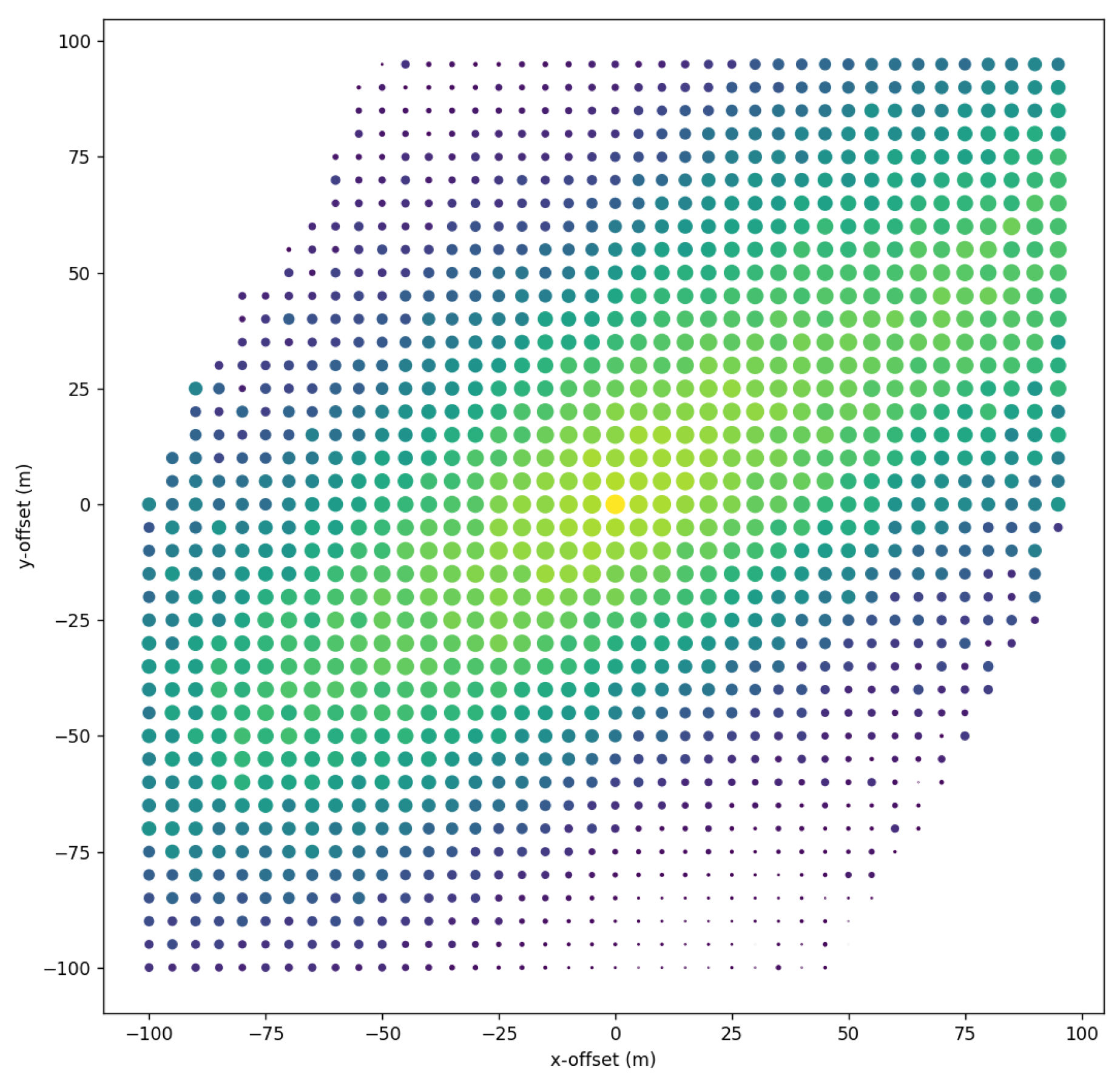
Figure 12.
Execution time of likelihood function against sub-sampling factor. Times are average result over 1000 iterations.
Figure 12.
Execution time of likelihood function against sub-sampling factor. Times are average result over 1000 iterations.
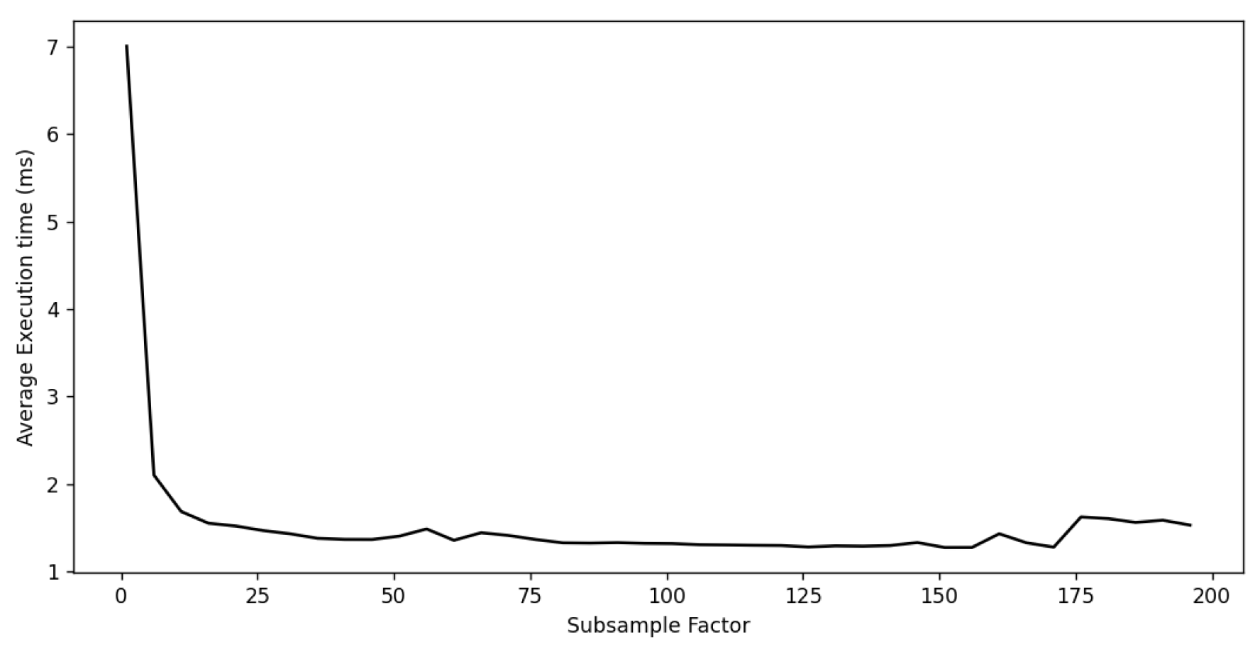
Figure 13.
Likelihood performance for sub-sampling factors of (a) 1,(b) 10,(c) 100.
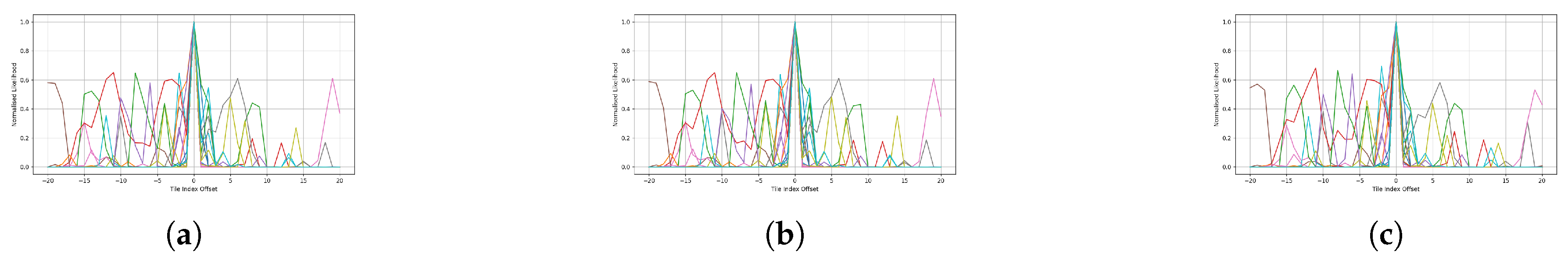
Figure 14.
Offset error between the estimated position and expected position for three control runs based on the return path dataset. (a) Particles 1000, Jitter 1.0 m, Sub-sampling 100. (b) Particles 5000, Jitter 5.0 m, Sub-sampling 10. (c) Particles 500, Jitter 5.0 m, Sub-sampling 1.
Figure 14.
Offset error between the estimated position and expected position for three control runs based on the return path dataset. (a) Particles 1000, Jitter 1.0 m, Sub-sampling 100. (b) Particles 5000, Jitter 5.0 m, Sub-sampling 10. (c) Particles 500, Jitter 5.0 m, Sub-sampling 1.
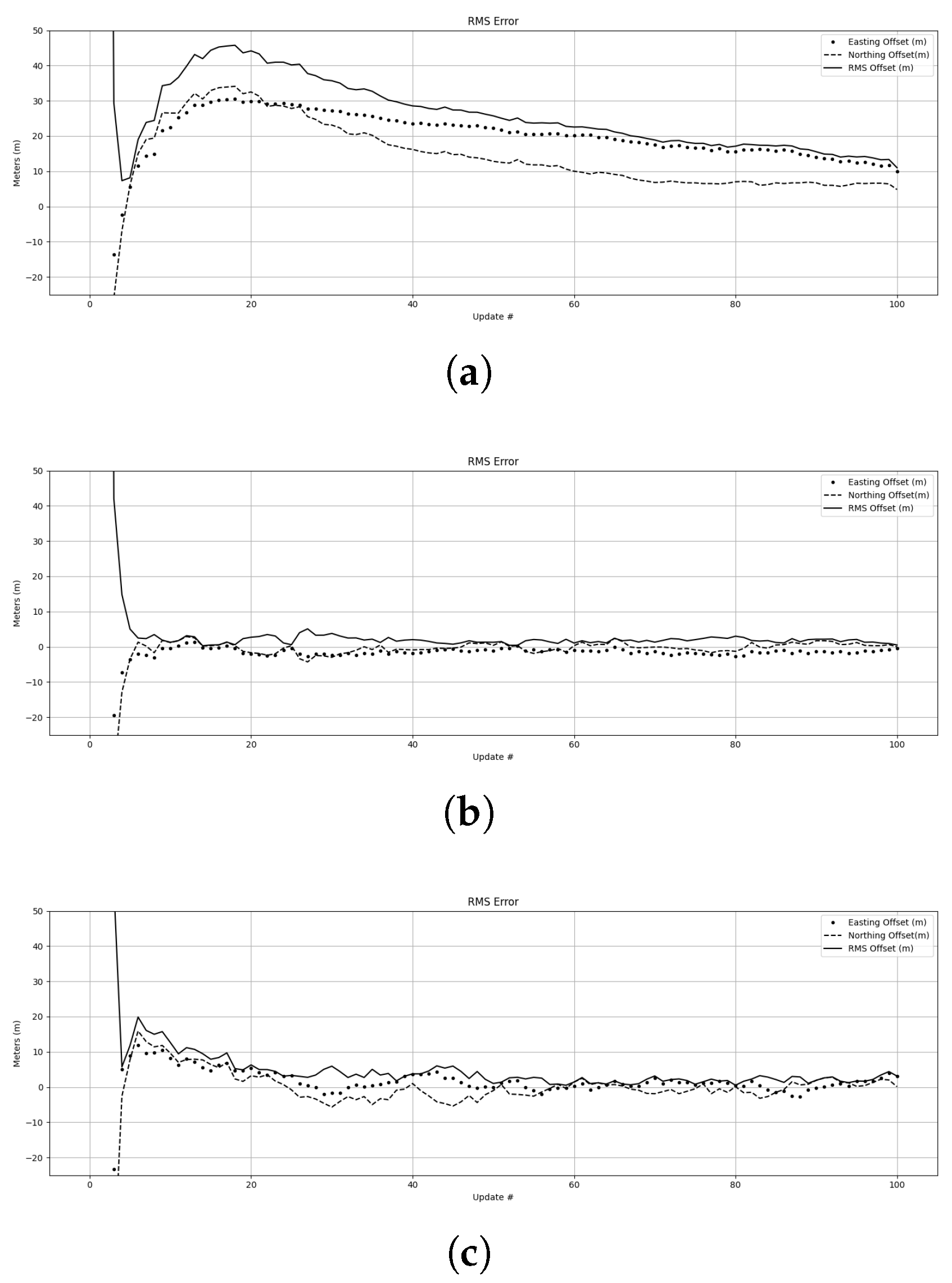
Figure 15.
Distribution of error against particle set sizes.
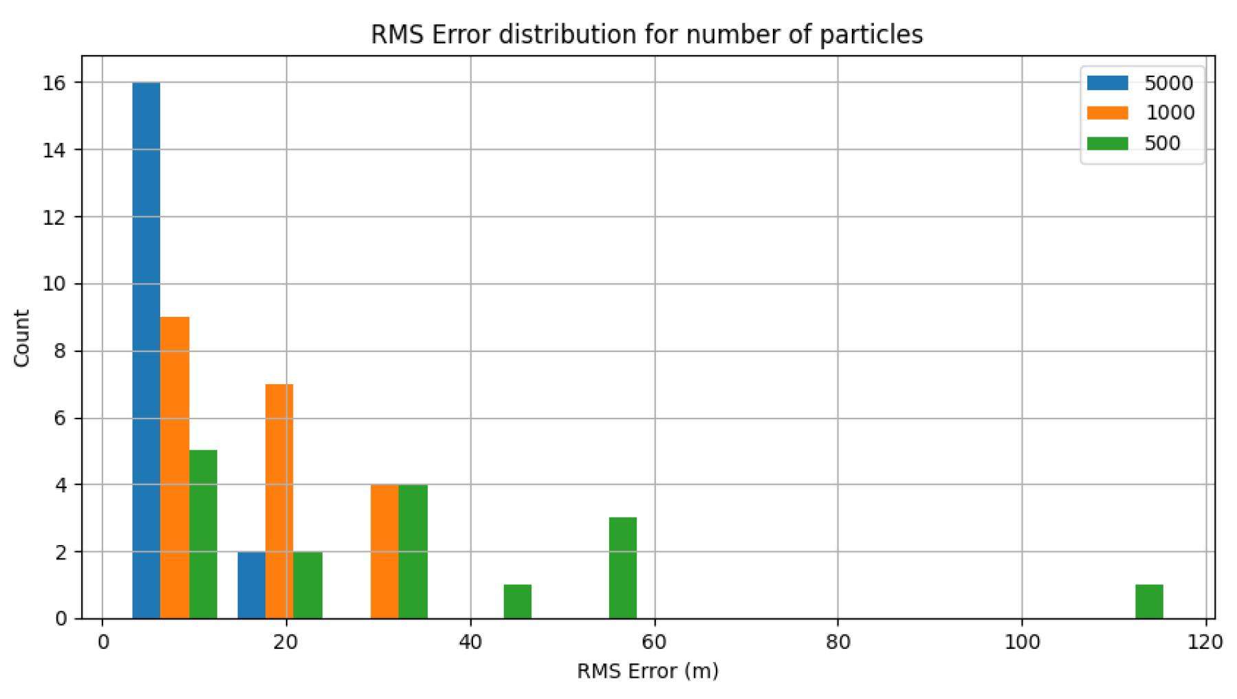
Figure 16.
Distribution of error against a set of particle set sizes.
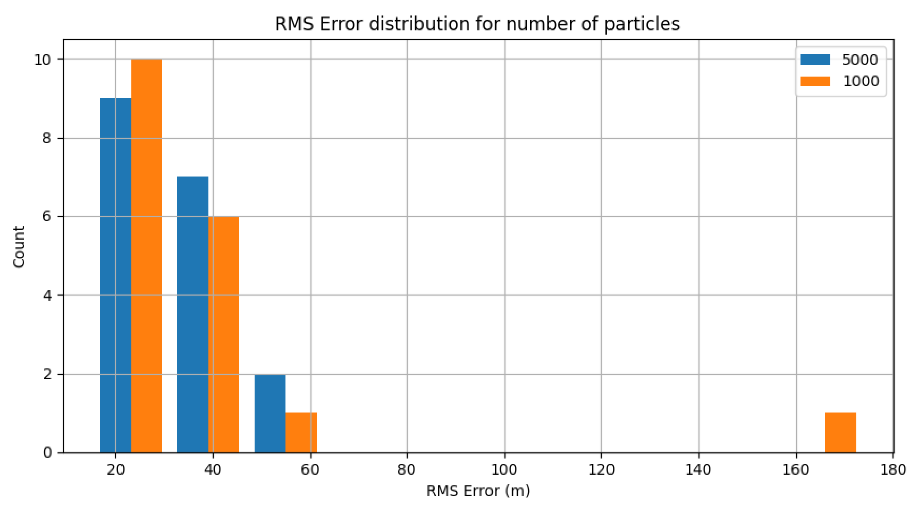
Figure 17.
(a) Out run as teach phase, return run as repeat. (b) Return run as teach phase, out run as repeat.
Figure 17.
(a) Out run as teach phase, return run as repeat. (b) Return run as teach phase, out run as repeat.
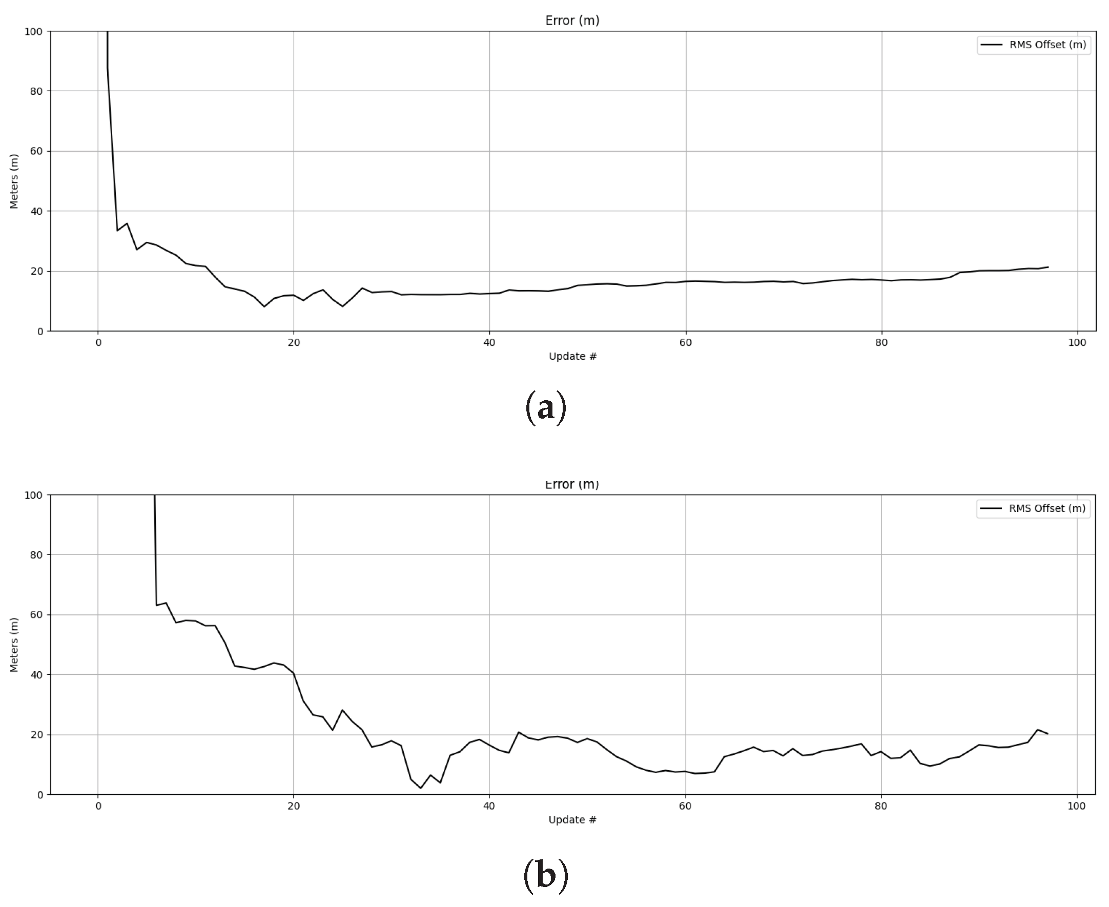

Table 1.
Conventions.
| Symbol | Name | Frame | Unit |
|---|---|---|---|
| N | North | NED | meters |
| E | East | NED | meters |
| Z | depth | NED | meters |
| Heading | NED | degrees | |
| x | x-position | Body | meters |
| y | y-position | Body | meters |
| z | range | Body | meters |
| u | forward speed | Body | meters-per-second |
| v | transverse speed | Body | meters-per-second |
| p | roll | Body | degrees |
| q | pitch | Body | degrees |
| r | yaw | Body | degrees |
Table 2.
Results of control tests.
| Particles | Jitter (m) | Sub-sample | N to converge | Error (m) | Maintained |
|---|---|---|---|---|---|
| 500 | 0.5 | 1 | 4 | 34.6 | Y |
| 10 | 4 | 51.6 | Y | ||
| 100 | 4 | 26.6 | Y | ||
| 1 | 1 | 4.5 | 72.7 | Y | |
| 10 | 4 | 36.4 | Y | ||
| 100 | Y | ||||
| 5 | 1 | 4 | 4.5 | Y | |
| 10 | 4.5 | 22.1 | Y | ||
| 100 | 5 | 8.6 | Y | ||
| 1000 | 0.5 | 1 | 3 | 24.9 | Y |
| 10 | 3 | 23.4 | Y | ||
| 100 | 4 | 18.0 | Y | ||
| 1 | 1 | 3.5 | 12.6 | Y | |
| 10 | 3 | 15.6 | Y | ||
| 100 | 3.5 | 18.6 | Y | ||
| 5 | 1 | 4 | 5.2 | Y | |
| 10 | 4 | 12.2 | Y | ||
| 100 | 3 | 7.9 | Y | ||
| 5000 | 0.5 | 1 | 4 | 6.4 | Y |
| 10 | 4 | 3.6 | Y | ||
| 100 | 4 | 8.2 | Y | ||
| 1 | 1 | 4 | 5.2 | Y | |
| 10 | 3.5 | 11.4 | Y | ||
| 100 | 3.5 | 10.0 | Y | ||
| 5 | 1 | 4 | 4.2 | Y | |
| 10 | 4 | 2.7 | Y | ||
| 100 | 4 | 3.7 | Y |
Table 3.
Results of tests.
| Particles | Jitter (m) | Sub-sample | N to converge | error (m) | Maintained |
|---|---|---|---|---|---|
| 1000.0 | 0.5 | 10.0 | 3.5 | 16.0 | Y |
| 1.0 | 10.0 | 3.0 | 101.2 | Y | |
| 5.0 | 10.0 | 2.5 | 31.9 | Y | |
| 5000.0 | 0.5 | 10.0 | 3.5 | 26.4 | Y |
| 1.0 | 10.0 | 3.0 | 24.8 | Y | |
| 5.0 | 10.0 | 3.5 | 37.5 | Y |
Disclaimer/Publisher’s Note: The statements, opinions and data contained in all publications are solely those of the individual author(s) and contributor(s) and not of MDPI and/or the editor(s). MDPI and/or the editor(s) disclaim responsibility for any injury to people or property resulting from any ideas, methods, instructions or products referred to in the content. |
© 2025 by the authors. Licensee MDPI, Basel, Switzerland. This article is an open access article distributed under the terms and conditions of the Creative Commons Attribution (CC BY) license (http://creativecommons.org/licenses/by/4.0/).
Copyright: This open access article is published under a Creative Commons CC BY 4.0 license, which permit the free download, distribution, and reuse, provided that the author and preprint are cited in any reuse.


