
Submitted:
24 July 2025
Posted:
25 July 2025
You are already at the latest version
Abstract
The Portfolio Selection process is addressed in a new methodology that incorporates advanced higher moment evaluation, fundamentals supported by robust Artificial Intelligence models. The Portfolio Intelligence (PI) model extracts hidden patterns from numerous financial statements and accounting information publicly availlablein a semi-strong efficiency, excluding effects of noise or fraud. PI is a challenging portfolio selection optimizer. The chaotic impact of speculative investors’ behaviours analyzed in fractal distributions, clean from noise on the PI model, provides a competing investment tool.
Keywords:
portfolio selection
; optimization
; financial analysis
; financial wellfare
; irrational investor behavior
; integrated systems
; radial basis functions
; support vector machines
; multi-layer perceptrons
; neural networks
; genetic algorithms
; nonlinear regressions
1. Introduction
The Epicurus, Ethical Hedonism, recently known von Neumann-Morgenstern axioms of choice subject to quadratic investor behavior on returns normally distributed , benchmark the portfolio selection discipline , as first described by Markowitz (1952) on the mean-variance criterion. Industry and academia in finance proved that neither of the two conditions holds (Merton, 2009). Investors have non-Normally Independently and Ideally Distributed returns and their utility is not quadratically distributed. Loukeris et al. (2008) noticed the marginal superiority of the Power over the Quadratic utility, incorporating skewness. As investors prefer positive skewness to ensure high profits from extremely positive events, Boyle and Ding (2005), and low kurtosis signaling low risk on extreme losses in the left side of the distribution, Athayde and Flores (2003); Ranaldo and Favre (2003), Lai et al. (2006). Loukeris (2008) Loukeris et al. (2014a, 2014b) showed higher reliability in investors’ preferences, demanding a more advanced analytical approach expressed in further higher moments. HyperKurtosis, m6, in the expected utility function E(U), decreases the investor’s uncertainty and exposure to various noise effects of systemic risk. Some of this noise is significant and is a by-product of illegal fraud in various forms. Subrahmanyam (2007) emphasizes that the theories of rational utility maximizers are a non-optimal alternative to behavior as they follow an ideal model far from real markets.
Hong et al. (2000) show that less news diffusion causes a momentum. Barberis et al. (2001) and Barberis and Huang (2001) used loss aversion in utility functions to show that stocks are guided by excess price fluctuations. Regarding investor moods, Shefrin and Statman (1984a) and Odean (1998) indicate a disposition effect among investors, who sell winners too soon and hold on to losers too long, although past winners do better than losers. Coval and Moskowitz (1999) prove the local optima limitations to mutual fund managers as they prefer investing in local companies, showing a proclivity for stocks headquartered in their region. Barberis and Shleifer (2003) note that the tendency of investors to heuristically categorize objects can lead to the emergence of style-based mutual funds. Hong et al. (2005) emphasize the strong impact of the word-of-mouth effect on portfolio decisions through social interactions between money managers. Various nonlinear parameters have a strong impact on investment performance: women’s conservatism, low trading frequency, weather, the day of the week, and a firm’s proximity to the investor can make a difference in investments.
The optimal selection problem is a two-phase process. Firstly, portfolio evaluation offers a feasible set that is largely inefficient and mostly rejected by risk-averse investors. The remaining efficient portfolios depend on investors’ behavior and are ranked on a utility function to receive the optimal portfolios. Second, the risk described in the variance, volatility, and hyperkurtosis is minimized.
The goal of this research is to examine the first phase of the optimization problem while offering a general solution to the second step and an integrated system capable of selecting and optimizing portfolios employing advanced methods of Artificial Intelligence and Finance. The single-period model is examined as I evaluate and introduce multiple different Radial Basis Functions networks, an MLP as a benchmark Support Vector Machine hybrid, and plain models of 11 different topologies each to produce the efficient frontier surface. The scope is quintuple, to:
- (I)
- investigate in-depth investors’ genitive behavior in higher moments, seeking more information on earnings and exposure to risk preferences.
- (II)
- introduce an improvement of the isoelastic utility as a more optimal function that supports higher moments.
- (III)
- extend Markowitz’s portfolio theory, evaluate the fundamentals, prices, and other available information, clear unnecessary noise, and determine healthy firms, excluding manipulation, fraud, etc.
- (IV)
- examine the efficiency of the AI networks in neuro-genetic hybrids or neural net forms on various topologies as a new learning process, compared to past results of Radial Basis Functions-RBF, Support Vector Machines-SVM, Multi-Layer Perceptrons-MLPs, defining the optimal model on firms’ classification to a dynamic, competitive investment portfolio.
- (V)
- introduce the integrated model PI as a modern solution to portfolio selection and optimization problems inspired by cutting-edge technologies.
The RBF, MLP neural networks, and SVM heuristics are examined on different neural forms and topologies and 11 hybrid forms, where genetic algorithms optimize their parameters. In these four variations, a new learning process, called the Batch, updates the trained weights of the model ex-ante, including new aspects of the training process at higher rates of convergence. The portfolio optimization problem is non-deterministic; hence, the most effective way to resolve it is through heuristics. I examine all the neural and hybrid RBF, MLP networks, and SVMs to define the most optimal classifier that will be used in the integrated system PI.
The complex human investment procedure cannot be accurately described in the markets, although I approach it through advanced isoelastic utility functions, fractal return distributions, and artificial intelligence.
The rest of the paper is organized as follows: Section 1 provides a description of the Efficient Market Hypothesis-EMH, higher moments, and the isoelastic utility I use. Section 2 offers the portfolio selection model of the isoelastic utility function, the new portfolio selection constraints with fundamentals, and Artificial Intelligence models. Section 3 presents the data analysis. Section 4 presents the results, and Section 5 concludes the paper.
2. Investments Behavior and Financial Modeling
Diversification rarely exists in real portfolios: investors own only a few stocks. The expected returns do not vary in the cross-section because of risk differentials across stocks. Existing empirical work is obsessed with data mining. Empirical research has confirmed out-of-sample evidence, both in terms of time periods and cross-sectionally across different countries. Nagel (2005) proves that mispricing is greatest for stocks where institutional ownership is lowest; Baker and Wurgler (2006) find that stocks that are difficult to arbitrage exhibit the maximum reversals in subsequent months when investor sentiment is high in a given period. Zhang (2006) shows that stocks in greater information uncertainty exhibit stronger statistical evidence of mispricing the predictability of returns from BE/ME and momentum within cross-sectional regressions.
Another parameter of investors’ actual behavioral problems is that risk theories do not appear to be strongly supported by the data. In markets, the theories of rational utility maximizers are unsatisfactory behavioral approaches because they examine how investors should behave, not how investors behave (Subrahmanyam, 2007). The evidence reveals that non-risk-related characteristics, such as stock return predictors, are far more compelling than risk-based characteristics.
In terms of attitude, overconfidence in private signals causes overreaction, the BE/ME effect, and long-run reversals, as self-attribution keeps overconfidence, permitting price overreaction and causing momentum. In the long run, Bayesian updating by agents reverses prices to fundamentals. Chan et al. (1996) argue that momentum is due to slow diffusion of news. Barberis et al. (1998) state that extrapolation from random sequences creates overreaction conservatism, the opposite of extrapolation, and creates momentum through underreaction. Hong and Stein (1999) suggest that the gradual diffusion of news causes momentum, and feedback traders who buy based on past returns create overreaction because they attribute the actions of past momentum traders to news, ending up purchasing too much stock that, when positions are reversed, causes momentum. Hong et al. (2000) find that stocks with fewer analysts following them have greater momentum, suggesting that less analyst following causes slower diffusion of news and more momentum, as in Hong and Stein (1999). Gervais and Odean (2001) model self-attribution bias in a dynamic set with learning and show that if this bias is influential, it may prevent a finitely-lived agent from ever learning about his true ability. Barberis et al. (2001) and Barberis and Huang (2001) attempted to incorporate loss aversion into the utility function. Barberis and Huang (2001) show that loss aversion in individual stocks leads to excess stock price fluctuations, as a BE/ME effect occurs because stocks with high BE/ME have performed well, requiring lower returns in equilibrium. Barberis et al. (2001) use similar arguments to justify the aggregate phenomena of excess volatility. Bernardo and Welch (2001) show that overconfidence in an economy is beneficial because increased risk-taking by overconfident agents facilitates the emergence of entrepreneurs who exploit new ideas. Barberis and Shleifer (2003) argue that the tendency of investors to heuristically categorize objects can lead to the emergence of style-based mutual funds. Scheinkman and Xiong (2003) show that agents with positive information may be tempted to buy overvalued assets because they believe they can sell that asset to agents with even more extreme beliefs in an analysis of the interaction between overconfidence and short constraints. Hirshleifer and Teoh (2003) model the notion that individual investors may have limited attention spans, which may cause them to miss certain important aspects of financial statements that are disclosed subtly and not directly, forcing dramatic valuation shifts when full and direct disclosure is made. Barberis et al. (2005) show that the S&P 500 betas of stocks increase when these stocks are added to the index and argue that this co-movement is partly because investors treat S&P stocks as belonging to one category. Grinblatt and Han (2005) argue that loss aversion can help explain momentum. Kausar and Taffler (2006) show that stocks initially exhibit continuation in response to an announcement that the firm is in distress but later exhibit reversals, supporting Daniel et al. (1998). Hong et al. (2006) show that overconfidence and short-sale phenomena can be exacerbated if assets have a limited float.
In terms of the psychological aspects of investors, Sorescu and Subrahmanyam (2006) test the Griffin and Tversky (1992) argument that agents overreact to the strength of a signal, using analyst experience and the number of categories spanned by analyst revisions as proxies for weight and strength, finding some support for this hypothesis. Regarding investor moods, Shefrin and Statman (1984a) examine the disposition effect among individual investors as a tendency to sell winners too soon and hold on to losers too long, but past winners do better than losers. Odean (1998) also found evidence of a disposition effect. DeLong et al. (1991) argue that irrational agents, being overconfident, can end up bearing more of the risk and can hence earn greater expected returns in the long run. Saunders (1993) found that the NYSE stock market tends to earn positive returns on sunny days, and returns are mediocre on cloudy days. Kyle and Wang (1997) argue that even if agents are risk-neutral, overconfidence acts as a precommitment to act aggressively, which causes the rational agent to scale back his trading activity, while in equilibrium, overconfident agents may earn greater expected profits than rational ones. Odean (1999) shows that individuals who trade the most are the worst at performing. Kamstra et al. (2000) note that returns around the weekend of the switch to standard time from daylight savings time are very negative, suggesting that induced depression from the switch among investors suffused with seasonal affective disorder causes the negative return. Barber and Odean (2001) prove that women outperform men in their individual stock investments because men, as hunter-gatherers, tend to be more overconfident than women. Hirshleifer and Shumway (2003) confirm this evidence across several international markets, concluding that investor mood affects the stock market. Gervais and Goldstein (2004) argue that overconfidence may permit better functioning of organizations. Goetzmann and Zhu (2005) find suggestive evidence that this effect is not due to the trading patterns of individual investors, leaving open the chance that it may arise from the market makers’ moods. Edmans et al. (2007) indicate that the outcomes of sporting events involving the country as a whole impact the country’s stock market. Hirshleifer et al. (2006) argue that when stock prices influence fundamentals by affecting corporate investment, irrational agents can earn greater expected profits than rational agents. Thus, the evidence in favor of inefficient financial markets is far more compelling than that in favor of efficient markets (Subrahmanyam, 2007). The magnitude of the effects is not large enough for retail investors to earn superior returns after accounting for transaction costs; however, institutions may be able to take advantage of such pricing problems. Colasante and Riccetti (2021) investigated how subjects consider the first four moments of return in making risky decisions from a very large heterogeneous population, finding that age and location are important determinants of risk in all domains, risk attitudes are correlated far from 1, with a larger risk aversion in non-financial contexts, and in a common risk trait, the financial risk propensity is positively correlated to the propensity to perform illegal activities.
Regarding portfolio selection, Coval and Moskowitz (1999) show that the preference for local stocks extends to mutual fund managers in the sense that such managers tend to show a proclivity for stocks headquartered in the region in which the managers are based. Benartzi and Thaler (2001) provide evidence of clearly irrational investor behavior, where investors follow a 1/n allocation rule across investment choices regardless of the stock-bond mix of the available choices. Grinblatt and Keloharju (2001b) indicate that Finnish agents are more prone to hold stock in firms that are located close to the investor. Goetzmann and Kumar (2003) show that individual investors who are young and less wealthy hold more under-diversified portfolios, suggesting that they may exhibit stronger behavioral biases. Benartzi and Thaler (2004) show that reducing investor autonomy by forcing investors to participate in a savings plan until they choose to opt out actually increases their savings rate. Hong et al. (2004) suggest that stock market participation is influenced by social interactions. Barber et al. (2004) find a wealth transfer from individuals to institutions via the stock market in the form of consumption—for the sheer pleasure of trading. However, agents fail to design sophisticated trading strategies. Frieder and Subrahmanyam (2005) show that individual investors prefer stocks with high brand recognition. Hong et al. (2005) argue that mutual fund managers are more likely to buy stocks that other managers in the same city buy, suggesting that portfolio decisions are affected by word-of-mouth between money managers.
CorporateEvents, Returns
Regarding the influence of corporate events on returns, long-run returns following events have been found to drift in the direction of short-term return reactions to the events. Grinblatt et al. (1984) and Desai and Jain (1997) find evidence of drift following stock splits. Bernard and Thomas (1989, 1990) reveal short-run post-earnings announcement stock price drifts in the direction indicated by earnings surprise. Loughran and Ritter (1995) and Spiess and Affleck-Graves (1995) conclude that after seasoned equity offerings, individual stock returns are poor and continue to be mediocre for more than a year following the offering. Loughran and Ritter (1995) find a negative drift after IPOs. Michaely et al. (1995) show that dividend initiations lead to positive drift and dividend cuts to the opposite. Stein (1996) discusses capital budgeting in irrational investors majorities that mis-assess the cash flow of the firm by a random amount; in case manager’s goal is to maximize the current stock price, then the discount rate should not be the CAPM rate, but one that adjusts the investor’s error, else if they maximize the long-run value, the hurdle rate CAPM of capital cost, as the beta in the CAPM uses the unobserved rational beta out of accounting data, as opposed to returns.
Teoh et al. (1998) present evidence in favor of the notion that managers manipulate earnings and investors do not entirely see through this activity. Daniel et al. (1998) show that managers time their issues to take advantage of misevaluation based on investors’ signals.
Baker & Wurgler (2000) show that return predictability from aggregate security issuances obtains at the market level as well. Brav et al. (2005) indicate, using survey evidence, that a significant consideration for repurchases among managers is precisely this sort of market timing. Subrahmanyam (2005) shows that managers with higher cognitive abilities have a greater tendency to misrepresent disclosures because they are less likely to get caught while lying, while an optimal compensation policy protects against fraud. Malmendier & Tate (2005a) suggest that an overconfident CEO will overinvest in his firm’s projects, believing that they are better than they actually are. Malmendier & Tate (2005b) consider the behavior of CEOs who win awards in the popular press, as it causes wasteful behavior that distracts from their jobs, in a poorly performance after the award granting both in terms of the stock price as well as accounting performance and also tend to manipulate earnings more than average.
In terms of the rationality characteristic, Daniel et al. (1998) assume that errors in information signals are correlated across agents. Barber and Odean (2002) find that investors who choose to make investments online are better performers than those who do not go online before the switch but are worse performers after the shift. Corwin and Coughenour (2005) argue that limited attention influences transaction costs. Barber et al. (2005) indicate that individual investor trading has a significant systematic component, suggesting that the biases of individuals do not cancel in aggregate. Hvidkjaer (2005) documents that the trade imbalances of small investors are negatively related to future stock returns in the cross-section. Kumar (2009a, 2009b) shows that investors tend to prefer stocks with lottery-like characteristics.
Hvidkjaer (2005) shows that small traders, on the net, buy loser momentum stocks and subsequently become net sellers of these stocks, suggesting that they may create momentum by underreacting to negative information. Hvidkjaer (2006) contradicts the notion that small investors overreact to information, and the reversal of their sentiment may cause stock return predictability. Thus, the imbalanced, unobtrusive information of the company to market prices can be evaluated through the model presented in this research and support investors in decision-making.
3. Higher Moments Addressing the Free Will of Investors
The returns distributions are not normally identically ideally distributed-n.i.i.d. in reality, and the Efficient Market Hypothesis-EMH does not hold, as various non-financial parameters affect stock prices. Investors are more sensitive to their potential losses (Subrahmanyam, 2007); thus, I will try to model the overall preferences, even those that incorporate the subconscious trends that guide them. Investors distribute their utility, balancing perceptions and fears on the one hand and earnings on the other. Their logic expects a rational amount of return, but the fear of loss is subconsciously magnified, producing remarkable decisions. The majority of investors are risk-averse or risk-neutral; hence, the fear parameter easily manipulates behaviors. In bullish periods, the fear of losing excess profits dominates, whereas, in bearish periods, the fear of maximizing losses influences non-rational herding behaviors. Loukeris et al. (2014a, 2014b, 2024) and Loukeris and Eleftheriadis (2024) introduced further moments than kurtosis as more accurate forms of gain and pain.
The initial problem of Philosophy and Science relies on the existence of Free Will from the cradle of civilization. Common sense accepts our full responsibility for the decisions we make despite the complexity of the limitations of liberty and will. Supporters of freedom will accept our freedom to act and choose. Whil Opposers declare that our will is not a product of our logic but rather of our nepotistic interests. Thus, Incompatibilists declare that determinism is hostile to freedom, and their perspective focuses on random effects, having common ground with Pink (2004) to the Skeptics whose thoughts conclude that freedom is impossible. Their opposers, the Compatibilists, accept the compatibility of freedom and determinism, agreeing partially with the Libertarians who accept freedom.
The free will idea Latham (2019) rejects the impossible status as systemically false, whilste Colasante and Riccetti (2021) concluded that the research now stops on the kurtosis because behaviors of higher orders are random, neglecting that the Subconscious brain reflects Ego affecting logic, and the Unconscious indeed produces random thoughts to Subconscious Loukeris and Eleftheriadis (2024), Loukeris et al. (2024). Nature is guided by this randomness.
Hence, further higher moments represent the detailed behavioral patterns on profit and loss non-linearly, under the fractal effects of chaotic entropy on prices, which is called random.
A more analytical tool that focuses on the details that define investing behaviors is introduced. Higher moments detect the hidden aspects of investors’ decision-making. Loukeris et al. (2014a, 2014b) noticed that on the implied utility function of the HARA family (Hyperbolic Absolute Risk Aversion), the 5th of hyperskewness and the 6th of hyperkyrtosis moments should be used in the form of
where
Hence, (1) is a series of higher-order moments that can be extended to the level of analysis that is desired. The general form of the normalized utility function is as follows:
where λν is the depth of accuracy on investors’ utility preferences toward risk, depending on the behavior, aλν a constant on investors’ profile: aλν = 1 for rational risk-averse individuals, aλν ≠ 1 for the non-rational, xi the value of return i in time t.
The Isoelastic Utility, a unique HARA function of Constant Relative Risk Aversion, is on risk-averse investors:
where W is wealth, and λ is a measure of risk aversion. Loukeris et al. (2014a, 2014b) indicated that the Markowitz model could have a broader alternative, relaxing its essential assumption on the normally distributed prices.
4. Methodology
4.1. Past Models
The initial convex problem of quadratic utility maximization, Markowitz (1952),
is insufficient in the real market. Maringer and Parpas (2009) considered the applicable higher-order moments:
where rp is the portfolio return, xi is the weight of asset i, ri is the return of the ith asset, μ is the mean, and σ2 is the variance.
4.2. Problem Definition
Fractal Behavior of Investors
The price trajectory among stock values follows a Fractal Distribution. The Fractal Distribution is a probabilistic self-similarity distribution over its parts and the whole in different scales. Fractals are natural phenomena that occur in marketsFractals demonstrate nonlinear characteristics and complex dynamic behaviors, thus, are more precise on the valuation of return and risk into the portfolios. The methods Li and Wu (2025) are in the price trajectory with endpoints x0 and xT, let e = d(x, y) be the distance between points x and y, as x1 and x2 the conditions d(x0, x1) = ε and d(x1, x2) = ε hold. If d(xn, xT) ≤ ε, the length of the trajectory is L(ε) = εn(ε). If ε is smaller, the curve length is more accurate. The fractal solution has values of d and m: , hold, exists, d, m ⋲ R+ are the fractal dimension and Minkowski capacity of the curve. The expectation is , of, where ρ(x) the density function, as returns follow a fractal allocation. Each fractal distribution is analyzed in four variables: (i) characteristic, (ii) skewness, (iii) scale, and (iv) location in higher complexity. If the characteristic < 2 and skewness = 0, the tail of the variable exhibits a fractal distribution:
In the fractal E(X) depends on 〈〉, thus Ef(X) = 〈〉 is the fractal expectation:
The variance is: Var(X) = (X) − [(X)if a≠3 (33). Similarly, if a ≠ 2 and a ≠ 3, the variance follows (34), in a < 3: Var(X) , (36) holds; when a > 3 and Var(X) is finite and still holds. Thus, in the fractal perspective Varf(X) = is the fractal variance.
Varf(Xi) is the fractal variance of the Xi random variable and follows the operational rule:
The portfolio P is composed of n assets with weights , and the return on the assets is :
The optimal portfolio of fractal expectation and variance reflects the weights of the assets {Yi
Fractal statistics can build portfolios and convert the weights of arrays to numerical values applied in portfolio selection, thereby building the fractal portfolio Li and Wu (2025).
As mentioned in the past by Loukeris and Eleftheriadis (2024), the non-convex area of solutions requires robust computational resources to detect the manipulation of the markets: cooked accounting, corporate hoax, rumors, that increase the risk, adjusting the excess return of the i optimal stock :
The preferences of investors are reflected in this problem.
Analytically:
Intuitively, the triple-filtered market data (accounting, sentiments, and chaos) are processed to provide the optimal portfolio with the highest financial wellfare. Wealth alone is insufficient to describe the overall needs of each investor, which may have a serene profile (loss and risk-averse), a neutral, or an aggressive speculative profile.
Loukeris et al. (2014a, 2014b) indicated the necessity of further higher moments in the model to optimally describe investors’ preferences. The problem is:
then
where υγ is the financial health of the company (binary: 0 toward bankruptcy, 1 healthy), and ετ is the heuristic model output, which is the evaluation result (binary: 0 healthy, or 1 distressed). The stocks that fail to fulfill all the previous superiority conditions are non-optimal stocks. Thus, given Loukeris et al. (2014a, 2014b) the previous is identical to
The non-convex problem requires strong heuristics to be solved. The new contribution is that I extract hidden accounting and financial patterns for a more thorough stock evaluation. Fraud and manipulation pose significant risks to investors. Thus, under (35), I filter distressed companies with no significant potential from portfolios. The evaluation υγ in (33) is more important than the investor’s risk behavior, as they have a reverse influence on υγ/λ. The minx f(x) equality in (34) declares that the categorical, objective influence of an asset is more influential than subjective investors’ behavior. The flowchart of the processes is shown in Figure 1.
4.3. The Portfolio Intelligence—PI Model
The integrated PI—Portfolio Intelligence model in the first step reads the fundamentals, accounting data, market prices, and preferred optimization period t.
Then, the initial method is selected to evaluate the companies whose stocks are candidates for the portfolio. In this step, the individual investor’s risk profile is given, and λ is selected for the isoelastic utility.
In the next step, the system examines whether this is the last firm to be examined and whether the condition for the optimal portfolio as an efficient portfolio is satisfied. I proceed to the next step of the initial evaluation, which uses a Computational Intelligence model to create two subsets: Subset A of healthy companies and Subset B of distressed firms.
In the specific model, I select the best network among the RBFs, SVMs, and MLPs. The ετ value is calculated (0 for healthy firms and 1 for distressed firms).
If ετ = 1, then the firm is distressed and is removed; if ετ = 0, the firm is healthy and is a candidate for the optimal efficient portfolio.
In the next step, Ut(Rt(i)), the utility function of (22), is calculated per firm.
Next, the firms are ranked according to their utility scores.
Then, the Efficient Frontier is calculated.
Next, firms with higher utility scores are selected for the efficient portfolio.
Sub-optimal and non-optimal firms are re-evaluated with potential new data in step 4 of CI evaluation, following all the steps.
Next, after the efficient portfolio is created, its Utility Function is calculated as UPj(f).
Then, the optimal overall portfolio U*Pj(f), whose utility is the maximum available, is detected, if possible, by all the available efficient portfolio utilities UPj(f) recorded in U*Pj(f)> UPj(f).
The process stops when the time limit is reached and the PI has the optimal portfolio.
The key idea is to filter out fraud and speculative noise that interfere with the price and disorient investors. Thus, by examining recent accounting entries and their financial indexes, I can define the real financial health of the firm. After the real healthy firms are selected then, their returns are considered on the model, and I proceed on the main core of the Markowitz initial approach, the detection of the efficient frontier and the creation of the efficient portfolio
The model’s flow chart is shown in Figure 1.
4.4. The Genetic Algorithms in the Neural Hybrids
The significance of each of the 16 financial inputs in all the Radial Basis Functions, Multi-Layer Perceptron networks, and Support Vector Machines is calculated using Genetic Algorithms on the Hybrid models only. These models are trained multiple times to detect the input combinations that produce the lowest errors. Genetic Algorithms are elaborated in four different hybrid models of different topologies, on:
- (i)
- the inputs layer only,
- (ii)
- the inputs and outputs layers only,
- (iii)
- all the layers,
- (iv)
- all the layers with cross-validation,
Batch learning was preferred to update the weights of the hybrid neuro-genetic JE after the presentation of the entire training set. Genetic Algorithms also resolved the problem of optimal values in all the hidden layers, and the output in:
- (a)
- the Step Size and
- (b)
- the Momentum Rate.
JE nets require multiple training sessions to achieve the lowest error.
5. Data
Data were produced from 1411 companies from the loan department of a Greek commercial bank, with the following 16 financial indices:
- (1)
- EBIT/Total Assets,
- (2)
- Net Income/Net Worth,
- (3)
- Sales/Total Assets,
- (4)
- Gross Profit/Total Assets,
- (5)
- Net Income/Working Capital,
- (6)
- Net Worth/Total Liabilities,
- (7)
- Total Liabilities/Total assets,
- (8)
- Long Term Liabilities/(Long Term Liabilities + Net Worth),
- (9)
- Quick Assets/Current Liabilities
- (10)
- (Quick Assets-Inventories)/Current Liabilities,
- (11)
- Floating Assets/Current Liabilities,
- (12)
- Current Liabilities/Net Worth,
- (13)
- Cash Flow/Total Assets,
- (14)
- Total Liabilities/Working Capital,
- (15)
- Working Capital/Total Assets,
- (16)
- Inventories/Quick Assets,
The 17th index was the initial classification done by bank executives, who determined if the company was in distress or healthy. The test set was 50% of the overall data, and the training set was 50%.
The key idea is to define and select the optimal network in terms of accuracy, efficiency, and impartiality regardless of the similar processing time of the trained networks
6. The Classifiers
6.1. Support Vector Machines
Support Vector Machines-(SVM) (Cortes and Vapnik (1995) produce
general regression and classification functions from a set of labeled training
data on a binary output since the input is categorical.
Training of SVMs is short in a sequential minimal optimization technique; the
output is unmarked, requiring a slow learning process in extended data of many
classes, minimum computations in the high dimensional space,
and processing directly of the input space. noted that for instances xi, i = 1,…l in labels yi ∈ 1, −1}, SVM are trained optimizing:
where, e is the vector of all 1, Q an l × l symmetric matrix of
under: 0 ≤ αi ≤ C, i= 1,…l, yT α = 0
K(xi, xj) is the kernel function, and C is the upper bound of all variables. In the case of unstable patterns, SVM rejects them as over-fitted, providing a statistically acceptable solution. The current SVM implements the Adatron kernel algorithm under the NeuroSolutions 2010 software, mapping inputs to a high-dimensional feature space, separating data into their respective classes, and isolating the inputs that fall close to the data boundaries. Hence, it effectively separates data sets that share complex boundaries. SVMs are trained by processing inputs near the decision surface. These SVM models elaborate Radial Basis Function–RBF Nets, Broomhead and Lowe (1988), Loukeris (2006, 2008), Loukeris et al. (2014a, 2014b) to put a Gaussian function at each data sample in backpropagation, creating a feature space that depends on the number of samples, while the large margin classifiers on training provide a fine generalization. The optimization problem of the Adatron learning algorithm for the RBFN substitutes the inner product of patterns in the input space by the kernel function:
in
αi ≥ 0, ∀i ∈ {1,…N} as g(xi) is:
and
in the choice of αi as a common starting multiplier, t as a small threshold, and h as a low learning rate. For M > t pattern, xi is selected, updating Δαι:
then,
The converging system produces a few αi ≠ 0, the support vectors, interacting with the closest boundary samples among classes. The Adatron kernel adjusts the RBFN Broomhead and Lowe (1988) in an optimal margin and prunes the RBF net so that its output for testing is
i ∈ support vectors. None of the 16 inputs had a predefined significance for the hybrid genetic SVMs. The Genetic Algorithms-GA Holland (1975/1992) selects important inputs, demanding multiple training of the network to define them, providing the minimum emphasis on the feature subset and SVM parameters. I examine multiple hybrid SVM models. The GAs were elaborated in different hybrids: (i) on the SVM inputs only, (ii) on the SVM outputs only, and (iii) on both the inputs and outputs. Batch learning was preferred for the weights after the presentation of the entire training set. All models were tested on 500 and 1000 epochs, respectively, to optimize the number of iterations upon convergence.
Feature selection was performed either on the filter or the wrapper approach Sun, Bebis, & Miller (2004) independent of the learning algorithm used to construct the classifier. The filter approach is computationally more efficient, but the wrapper approach, although slower, selects features more optimally. In bankruptcy prediction, feature subset selection plays an important role in prediction performance. Furthermore, its importance increases when the number of features is large. This paper seeks to improve the SVM-based bankruptcy prediction model. I propose a GA as the method of feature subset selection in the SVM system. This paper uses the wrapper approach to select the optimal feature subset of the SVM model using GA. The increase function is selected to terminate training under the Cross-Validation set when its MSE increases, avoiding overtraining, while the best training weights are loaded onto the test set. The GA solved the optimal values problem in (a) the number of neurons (Processing Elements-, PE), (b) Step Size, and (c) Momentum Rate, requiring multiple trainings of the network to conclude the lowest error mode. In the case of the models with GA on the output layer, the value of the Step size and Momentum were optimized.
As observed, a higher number of epochs allowed the iterations to provide a more thorough analysis of the network. The overall classification of these SVM models was excellent, taking the bank experts initial opinion as a benchmark, with a fine performance in almost all the model parameters, which failed to reduce overtraining hazard in almost all different SVM hybrid or SVM models, questioning the models’ independence and impartiality. Overall, the Hybrid SVM of 1000 epochs GA optimization on the inputs and Cross-Validation converged optimally in terms of classification and performance, with a significant overtraining hazard but in excess computation time. The Hybrid SVM of 500 epochs of inputs Genetic Algorithms optimization almost similar qualities in less time, and the third rank is given to the SVM of 1000 that in all sets remained very reliable on the highest overfitting hazard but a very fast computational time. These models are quite useful for all profiles of investors, emphasizing either accuracy or speed, while the overfitting aspect must be considered.
A comparative analysis of the SVM results (Table 2) to the MLP, which is a basic Neural Network, clearly shows the higher classification capabilities of the SVM models that face the criticism of partiality on the model’s behavior toward the supervisor and the underperformance of the MLP that was ranked last in terms of classification and efficiency but did not face questions on integrity.
6.2. Radial Basis Functions
Radial Basis Function (RBF) nets Broomhead and Lowe (1988) are a linear model of regressions, classifications, and time series predictions in supervised learning. The training set, or set of examples, contains the independent (input) variable, which is sensitive to noise, and the dependent (output) variable. The Linear models are:
where f(x) is a linear combination of m set of fixed functions, the Basis Functions, wj linear combination coefficients, and hj weights. A Radial Basis Function (RBF) network, has every input component (p) on a hidden node layer, and each node is a p multivariate Gaussian function (RBF):
of mean xi and variance, the linear weight on the hidden nodes produces an output that may create a very large hidden layer:
Hybrid RBFNs in Genetic Algorithms
The significance of each financial index of the 16 inputs in the hybrid RBF network, Broomhead and Lowe (1988), is unknown to the model; hence, Genetic Algorithms, Holland (1975/1992), selects them. Each model was trained multiple times to define the input combination with the lowest error. Genetic Algorithms were implemented in different hybrid models: (i) on the input layer only, (ii) on the input and output layers only, (iii) into all the layers and cluster centers, and (iv) into all the layers and cluster centers with cross-validation, in different topologies. Batch learning was selected to update the weights of the hybrid neuro-genetic RBF after the presentation of the entire training set. The competitive rule was the Conscience Full function in the Euclidean metric, as the conscience mechanism keeps a count of how often a neuron wins the competition and enforces a constant winning rate across the neurons. There were four neurons per hidden layer, using the TanhAxon transfer function, on the momentum learning rule. Genetic Algorithms resolved the problem of optimal values in (a) Processing Elements, (b) Step Size, (c) Momentum Rate, and (d) Cluster Centers. RBF nets require multiple training sessions to obtain the lowest error. The output layer elaborated on Genetic Algorithms in some hybrids, optimizing the Step size and Momentum.
In terms of overall performance, Loukeris et al. (2008 2014a, 2014b) found that the Hybrid RBF on GA optimization into inputs and outputs only with three hidden layers had the overall optimal performance, where 97.24% and 72.48% of the companies converged in classification as healthy and distressed, respectively. The fitness of the model to the data was high at r = 0.925, while errors remained low at MSE = 0.116, NMSE = 0.393, in error 9.039% on a moderate Akaike criterion, in a short computing time of 5 h 48 min 56 s (Table 1, Table 2 and Table 3).
The second place was given to the Hybrid RBF of GAs in all layers of no hidden layers where 98.15% of healthy and 60.09% of distressed companies were correctly classified, in a fine fitness to the data at 0.815 in medium MSE, NMSE, proportional errors, medium AIC signifying statistical non-impartiality, in a quick processing time of 5 h 2 min 28 s (Table 3).
The third rank is given to the SVM of 500 epochs that excelled in classification and performance; however, the extremely high partiality bias it incorporates is a serious point of discussion. Table 3.
The SVM of 1000 epochs ranked fourth for the same reasons as the 3rd. The MLP had the worst results overall, although it is a reliable network with significant impartiality, as shown in Table 3.
The integrated PI model is fully flexible as I provide the user with the opportunity to select whether the financial health of the firms is performed once and to choose the type of the model (neural net, hybrid net, models with cross-validation), or twice by an initial neural net and then by a hybrid net of CV in a double precision process.
The reason I provide these alternatives is that given that the neural net operates as a black box with unique results each time, I try to avoid misjudgment due to the nonlinear complexity of the models and overfitting in the absence of Cross-Validation. In the case of a single precision with a hybrid that includes Cross-Validation, the models are secured by the risk of overfitting but are exposed to the risk of non-repeatable objectivity.
Thus, in the case of double-precision models, the user is ensured that the financial health is found accurately and objectively.
7. Conclusions and Future Research
The integrated model PI—Portfolio Intelligence, offers a more detailed approach to the real-time portfolio selection problem. The main advantage of this system is that by extracting hidden patterns, it tries to overcome manipulation and speculation games. Radial Basis Function networks have a promising performance of high calibration, which allows them to be a part of this model or its future developments. Moreover, the Hybrid Radial Basis Function on GA optimization into inputs and outputs only with three hidden layers had the overall optimal performance as a reliable model of good classification capabilities, performance, and low computing time but had a higher risk of overfitting, while the Hybrid RBF of GAs in all layers of no hidden layers in a marginally lower rank was the best option in all aspects, and it protected from overtraining.
Support Vector Machines have excellent overall classification and performance, but they are exposed to partiality features and are thus not appropriate for numeric classification problems. Thus, the Radial Basis Function networks provide a good nonlinear regression for Portfolio Selection.
In terms of investment intuition, the triple-filtering of market data (chaos, accounting, and sentiments) combines hidden information to process and optimize the portfolio per investor to the highest appropriate financial welfare. Only the wealth aspect is insufficient to describe the overall needs of each investor, which may have a serene profile (loss and risk-averse), a neutral, or an aggressive speculative profile. The financial welfare of investors in terms of free will in decision-making is expressed in advanced moments that reflect Aristotle’s Logic in consecutive induction, and Epicurus seeks Hedonism (serenity) as the customary behavior of daily routine is challenged by dynamic logic to achieve higher goals. Investors with limited information affected by personal bias usually exhibit irrational patterns.
The Portfolio Intelligence (PI) model supports the holistic protection of investors through a thorough portfolio optimization process.
Author Contributions
This paper was prepared as follows: Material preparation, and analysis were performed by N. Loukeris. data collection N. Loukeris & L. Maltoudoglou The first draft of the manuscript was written by N. Loukeris. Supervision and additional writing was done by Y. Boutalis, I. Eleftheriadis & G. Gikas. All authors read and approved the final manuscript.
Funding
An initial form of this work was supported by ELKE Grant as follows: Author I. have received research support from the Democritus University of Thrace for participation at the IEEE 6th International Conference on Information, Intelligence, Systems and Applications, IISA2015, Ionian University, Corfu, Greece, July 6–8. The authors declare that no funds, grants, or other support were received during the preparation of this manuscript.
Institutional Review Board Statement
Accepted principles of ethical and professional conduct have been followed.
Informed Consent Statement
Data Availability Statement
Availlable upon request
Conflicts of Interest
Financial interests: Authors by from the and declare they have no financial interests. Authors from have received speaker and travel support from ELKE fund of the Democritus University of Thrace. Non-financial interests. No conflicts of interest exist between authors or third parties.
References
- Athayde, G., & Flores, R. (2003). Incorporating skewness and Kurtosis in portfolio optimization: A multidimensional efficient set. In S. Satchell, & A. Scowcroft (Eds.), Advances in portfolio construction and implementation (pp. 243–257). Butterworth-Heinemann.
- Baker, M., & Wurgler, J. (2000). The equity share in new issues and aggregate stock returns. Journal of Finance, 55, 2219–2257. [CrossRef]
- Baker, M. P., & Wurgler, J. (2006). Investor sentiment and the cross–section of stock returns. Journal of Finance, 61, 1645–1680.
- Barber, B., Lee, Y. T., Liu, Y. J., & Odean, T. (2004). Who gains from trade? Evidence from Taiwan. Working Paper. University of California at Berkeley.
- Barber, B., & Odean, T. (2001). Boys will be boys: Gender, overconfidence and common stock investment. Quarterly Journal of Economics, 116, 261–292.
- Barber, B., & Odean, T. (2002). Online investors: Do the slow die first? Review of Financial Studies, 15, 455–488.
- Barber, B., Odean, T., & Zhu, N. (2005). Systematic noise. Working Paper. University of California at Davis.
- Barberis, N., & Huang, M. (2001). Mental accounting, loss aversion, and individual stock returns. Journal of Finance, 56, 1247–1292. [CrossRef]
- Barberis, N., Huang, M., & Santos, J. (2001). Prospect theory and asset prices. Quarterly Journal of Economics, 141, 1–53.
- Barberis, N., & Shleifer, A. (2003). Style investing. Journal of Financial Economics, 68, 161–199.
- Barberis, N., Shleifer, A., & Vishny, R. (1998). Model of investor sentiment. Journal of Financial Economics, 49, 307–343.
- Barberis, N., Shleifer, A., & Wurgler, J. (2005). Comovement. Journal of Financial Economics, 75, 283–317.
- Benartzi, S., & Thaler, R. (2004). Save more tomorrow: Using behavioural economics to increase employee saving. Journal of Political Economy, 112, 164–187. [CrossRef]
- Benartzi, S., & Thaler, R. H. (2001). Naive diversification strategies in defined contribution saving plans. American Economic Review, 91, 79–98. [CrossRef]
- Bernard, V. L., & Thomas, J. K. (1989). Post-earnings-announcement drift: Delayed price response or risk premium? Journal of Accounting Research, Supplement, 27, 1–48.
- Bernard, V. L., & Thomas, J. K. (1990). Evidence that stock prices do not fully reflect the implications of current earnings for future earnings. Journal of Accounting and Economics, 13, 305–340. [CrossRef]
- Bernardo, A., & Welch, I. (2001). On the evolution of overconfidence and entrepreneurs. Journal of Economics and Management Strategy, 10, 301–330.
- Boyle, P., & Ding, B. (2005). Portfolio selection with skewness. In M. Breton, & H. Ben-Ameur (Eds.), Numerical methods in finance. GERAD Groupe D’études et de Recherche en Analyse des Decisions, Springer.
- Brav, A., Graham, J. R., Harvey, C. R., & Michaely, R. (2005). Payout policy in the 21st century. Journal of Financial Economics, 77, 483–427.
- Broomhead, D. S., & Lowe, D. (1988). Multivariable functional interpolation and adaptive networks. Complex Systems, 2, 321–355.
- Chan, L. K., Jegadeesh, N., & Lakonishok, J. (1996). Momentum strategies. Journal of Finance, 51, 1681–1714.
- Colasante, A., & Riccetti, L. (2021). Financial and non-financial risk attitudes: What does it matter? Journal of Behavioral and Experimental Finance, 30, 100494.
- Cortes, C., Vapnik, V. Support-vector networks. Mach Learn 20, 273–297 (1995). [CrossRef]
- Corwin, S., & Coughenour, J. (2005). Limited attention and the allocation of effort in securities trading. Working Paper. University of Notre Dame. [CrossRef]
- Coval, J. D., & Moskowitz, T. J. (1999). Home bias at home: Local equity preference in domestic portfolios. Journal of Finance, 54, 145–166. [CrossRef]
- Daniel, K. D., Hirshleifer, D., & Subrahmanyam, A. (1998). Investor psychology and security market under and over-reactions. Journal of Finance, 53, 1839–1886. [CrossRef]
- DeLong, J. B., Shleifer, A., Summers, L., & Waldmann, R. J. (1991). The survival of noise traders in financial markets. Journal of Business, 64, 1–20. [CrossRef]
- Desai, H., & Jain, P. C. (1997). Long-run common stock returns following stock splits and reverse splits. Journal of Business, 70, 409–434. [CrossRef]
- Edmans, A., Garcia, D., & Norli, O. (2007). Sports sentiment and stock returns. Journal of Finance, 62, 1967–1998. [CrossRef]
- Frieder, L., & Subrahmanyam, A. (2005). Brand perceptions and the market for common stock. Journal of Financial and Quantitative Analysis, 40, 57–85. [CrossRef]
- Gervais, S., & Goldstein, I. (2004). Overconfidence and team coordination. Working Paper. University of Pennsylvania.
- Gervais, S., & Odean, T. (2001). Learning to be overconfident. Review of Financial Studies, 14, 1–27. [CrossRef]
- Goetzmann, W., & Zhu, N. (2005). Rain or shine: Where is the weather effect? European Financial Management, 11, 559–578.
- Goetzmann, W. N., & Kumar, A. (2003). Why do individual investors hold underdiversified portfolios? Working Paper. Yale ICF.
- Griffin, D., & Tversky, A. (1992). The weighing of evidence and the determinants of overconfidence. Cognitive Psychology, 24, 411–435. [CrossRef]
- Grinblatt, M., & Han, B. (2005). Prospect theory, mental accounting, and momentum. Journal of Financial Economics, 78, 311–339.
- Grinblatt, M., & Keloharju, M. (2001a). How distance, language and culture influence stockholdings and trades. Journal of Finance, 56, 1053–1073.
- Grinblatt, M., & Keloharju, M. (2001b). What makes investors trade? Journal of Finance, 56, 589–616.
- Grinblatt, M., Masulis, R. W., & Titman, S. (1984). The valuation effects of stock splits and stock dividends. Journal of Financial Economics, 13, 97–112. [CrossRef]
- Hirshleifer, D., & Shumway, T. (2003). Good day sunshine: Stock returns and the weather. Journal of Finance, 58, 1009–1032. [CrossRef]
- Hirshleifer, D., Subrahmanyam, A., & Titman, S. (2006). Feedback and the success of irrational traders. Journal of Financial Economics, 81, 311–388.
- Hirshleifer, D., & Teoh, S. H. (2003). Limited attention, information disclosure, and financial reporting. Journal of Accounting & Economics, 36, 337–386.
- Holland, J. (1992). Adaptation in natural and artificial system. MIT Press. First edition 1975 Michigan University Press. (Original work published 1975). ISBN 978-0262581110.
- Hong, H., Kubik, J., & Stein, J. (2004). Social interactions and stock market participation. Journal of Finance, 59, 137–163. [CrossRef]
- Hong, H., Kubik, J., & Stein, J. (2005). Thy neighbor’s portfolio: Word-of-mouth effects in the holdings and trades of money managers. Journal of Finance, 60, 2801–2824.
- Hong, H., Lim, T., & Stein, J. (2000). Bad news travels slowly: Size, analyst coverage and the profitability of momentum strategies. Journal of Finance, 55, 265–295.
- Hong, H., Scheinkman, J., & Xiong, W. (2006). Asset float and speculative bubbles. Journal of Finance, 61, 1073–1117. [CrossRef]
- Hong, H., & Stein, J. C. (1999). A unified theory of underreaction, momentum trading and overreaction in asset markets. Journal of Finance, 54, 2143–2184.
- Hvidkjaer, S. (2005). Small trades and the cross-section of stock returns. Working Paper. University of Maryland. [CrossRef]
- Hvidkjaer, S. (2006). A trade-based analysis of momentum. Review of Financial Studies, 19, 457–491. [CrossRef]
- Jean, W. H. (1973). More on multidimensional portfolio analysis. Journal of Financial and Quantitative Analysis, 8(3), 475–490.
- Kamstra, M. J., Kramer, L. A., & Levi, M. D. (2000). Losing sleep at the market: The daylight-savings anomaly. American Economic Review, 90, 1005–1011. [CrossRef]
- Kausar, A., & Taffler, R. (2006). Testing behavioral finance models of market under and overreaction: Do they really work? Working Paper. University of Edinburgh.
- Kumar, A. (2009a). Hard-to-Value stocks, behavioral biases, and informed trading. Journal of Financial and Quantitative Analysis, 44, 1375–1401.
- Kumar, A. (2009b). Who gambles in the stock market? Journal of Finance, 54, 1889–1933.
- Kyle, A., & Wang, F. A. (1997). Speculation duopoly with agreement to disagree: Can overconfidence survive the market test? Journal of Finance, 52, 2073–2090.
- Lai, K. K., Yu, L., & Wang, S. (2006, June 20–24). Mean-variance-skewness-kurtosis-based portfolio optimization (Vol. 2, pp. 292–297). First International Multi-Symposiums on Computer and Computational Sciences (IMSCCS’06), Hangzhou, China.
- Latham, A. J. (2019). The conceptual impossibility of free will error theory. European Journal of Analytic Philosophy, 15, 99–120. [CrossRef]
- Li, K., & Wu, X. (2024). Research on the optimization of commercial bank technology credit asset portfolio model under fractal distribution. Computational Economics, forthcoming. [CrossRef]
- Loughran, T., & Ritter, J. (1995). The new issues puzzle. Journal of Finance, 50, 23–52.
- Loukeris, N., & Matsatsinis, N. (2006). Corporate financial evaluation and bankruptcy prediction implementing artificial intelligence methods. WSEAS Transactions on Business and Economics, 4(3), 938–942.
- Loukeris, N. (2008). Radial basis functions networks to hybrid neuro-genetic RBF Networks in financial evaluation of corporations. International Journal of Computers, 2(2), 812–819.
- Loukeris, N., & Eleftheriadis, I. (2012, August 1–5). Bankruptcy prediction into hybrids of time lag recurrent networks with genetic optimisation, multilayer perceptrons neural nets, and bayesian logistic regression [Research Paper Award]. Proceedings of the International Summer Conference of the International Academy of Business and Public Administration Disciplines (IABPAD), Library of Congress, Honolulu, HI, USA, ISSN 547-4836.
- Loukeris, N., & Eleftheriadis, I. (2013, December 12–15). A novel approach on hybrid support vector machines into optimal portfolio selection. IEEE International Symposium on Signal Processing and Information Technology, Athens, Greece.
- Loukeris, N., & Eleftheriadis, I. (2024) Optimal investments in the Portfolio Yield Reactives (PYR). Journal of Risk Financial Management, 17(8), 376. [CrossRef]
- Loukeris, N., Eleftheriadis, I., Boutalis, Y., & Gikas, G. (2024). Optimizing portfolio in the evolutional portfolio optimization system (EPOS). Mathematics, 12(17), 2729. [CrossRef]
- Loukeris, N., Eleftheriadis, I., & Livanis, E. (2014a, July 1–3). Optimal asset allocation in radial basis functions networks, and hybrid neuro-genetic RBFΝs to TLRNs, MLPs and bayesian logistic regression. World Finance Conference, Venice, Italy.
- Loukeris, N., Eleftheriadis, I., & Livanis, E. (2014b, July 7–9). Portfolio selection into radial basis functions networks and neuro-genetic RBFN hybrids. IEEE 5th International Conference on Information, Intelligence, Systems and Applications IISA, Chania, Greece.
- Malmendier, U., & Tate, G. A. (2005a). CEO overconfidence and corporate investment. Journal of Finance, 60, 2661–2700. [CrossRef]
- Malmendier, U., & Tate, G. A. (2005b). Superstar CEOs. Working Paper. Stanford University.
- Maringer, D., & Parpas, P. (2009). Global optimization of higher order moments in portfolio selection. Journal of Global Optimization, 43, 219–230. [CrossRef]
- Markowitz, H. M. (1952). Portfolio selection. Journal of Finance, 7(1), 77–91.
- Merton, R. C. (2009). Continuous-time finance (revised edition, 1992 ed). Blackwell.
- Michaely, R., Thaler, R. H., & Womack, K. L. (1995). Price reactions to dividend initiations and omissions: Overreaction or drift? Journal of Finance, 50, 573–608.
- Nagel, S., (2005), Short sales, institutional investors and the cross-section of stock returns, Journal of Financial Economics, Volume 78, Issue 2, 277-309, ISSN 0304-405X. [CrossRef]
- Odean, T. (1998). Are investors reluctant to realize their losses? Journal of Finance, 53, 1775–1798.
- Odean, T. (1999). Do investors trade too much? American Economic Review, 89, 1279–1298.
- Orr, G. (1999). Neural networks. Willamette University.
- Pink, T. (2004). Free will: A very short introduction. Oxford University Press.
- Principe, J., de Vries, B., Kuo, J., & Oliveira, P. (1992). Modeling applications with the focused gamma network. Neural Information Processing Systems, 4, 121–126.
- Saunders, J. (1993). Stock prices and wall street weather. American Economic Review, 83, 1337–1345.
- Scheinkman, J. A., & Xiong, W. (2003). Overconfidence, short-sale constraints, and bubbles. Journal of Political Economy, 111, 1183–1219.
- Shefrin, H., & Statman, M. (1984a). The disposition to sell winners too early and ride losers too long: Theory and evidence. Journal of Finance, 40, 777–790.
- Sorescu, S., & Subrahmanyam, A. (2006). The cross section of analyst recommendations. Journal of Financial and Quantitative Analysis, 41, 139–168.
- Spiess, D. K., & Affleck-Graves, J. (1995). Underperformance in long-run stock returns following seasoned equity offerings. Journal of Financial Economics, 38, 243–268. [CrossRef]
- Stein, J. (1996). Rational capital budgeting in an irrational world. Journal of Business, 69, 429–455. [CrossRef]
- Subrahmanyam, A. (2005). A cognitive theory of corporate disclosures. Financial Management, 34, 5–33. [CrossRef]
- Subrahmanyam, A. (2007). Behavioral finance: A review and synthesis. European Financial Management, 14, 12–29.
- Teoh, S. H., Welch, I., & Wong, T. J. (1998). Earnings management and the underperformance of seasoned equity offerings. Journal of Financial Economics, 50, 63–99. [CrossRef]
- Zhang, X. F. (2006). Information uncertainty and analyst forecast behavior. Journal of Finance, 61, 105–136.
Figure 1.
The proposed model.
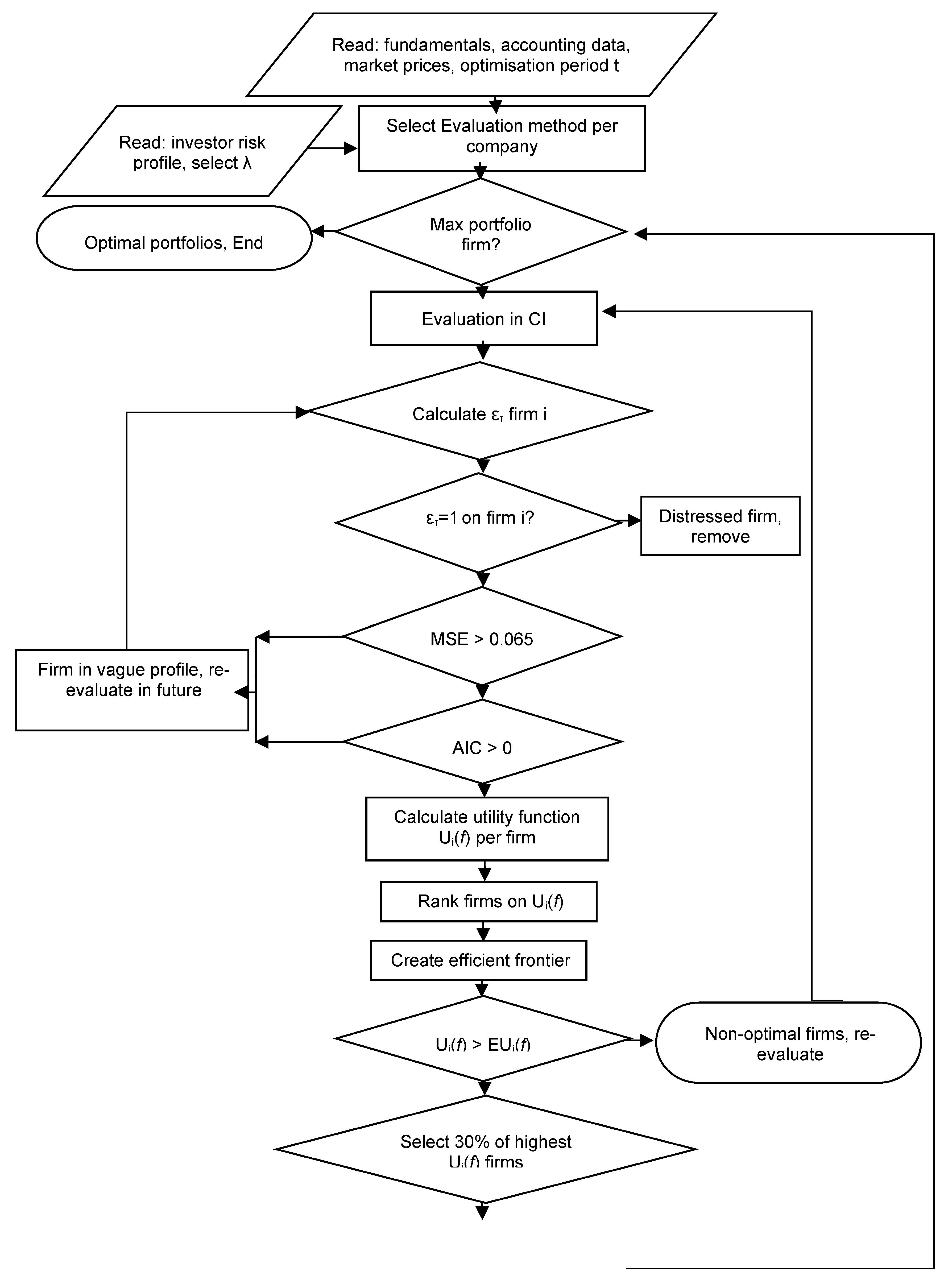
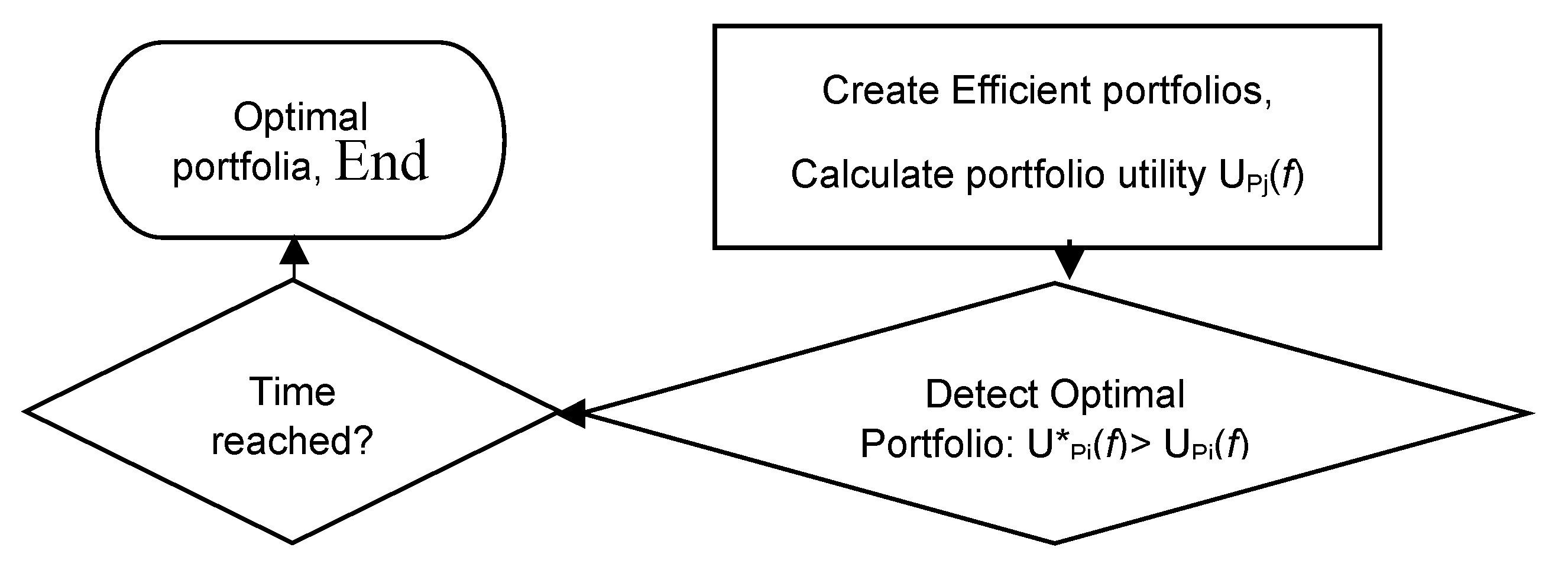

Table 1.
RBFs Overall Optimal Results Loukeris et al. (2014a).
| Hybrid Networks | Active Confusion Matrix | Performance | Time | |||||||||
|---|---|---|---|---|---|---|---|---|---|---|---|---|
| Layers | 0→0 | 0→1 | 1→0 | 1→1 | MSE | NMSE | R | %Error | AIC | MDL | ||
| RBF input-output GA | 3 | 97.24 | 2.76 | 27.52 | 72.48 | 0.166 | 0.393 | 0.9256 | 9.039 | 672.93 | 1912.74 | 5 h 48′56″ |
| RBF GA | 0 | 98.15 | 1.85 | 39.91 | 60.09 | 0.188 | 0.445 | 0.8158 | 13.009 | 37.12 | 820.831 | 5 h 02′28″ |
| RBF inputs GA | 0 | 97.73 | 2.26 | 46.32 | 53.67 | 0.219 | 0.519 | 0.7916 | 12.383 | 282.78 | 1154.02 | 4 h 19′42″ |
Table 2.
Overall Optimal Results on SVMs, RBFs MLPs, Loukeris and Eleftheriadis (2012), Loukeris et al. (201 2014a).
Table 2.
Overall Optimal Results on SVMs, RBFs MLPs, Loukeris and Eleftheriadis (2012), Loukeris et al. (201 2014a).
| Neural Network | Active Confusion Matrix | Performance | Time | |||||||||
|---|---|---|---|---|---|---|---|---|---|---|---|---|
| Layers | 0→0 | 0→1 | 1→0 | 1→1 | MSE | NMSE | r | %Error | AIC | MDL | ||
| SVM 500 epochs | 100 | 0 | 0 | 100 | 0.035 | 0.072 | 0.999 | 5.436 | 23,073.68 | 39,305.4 | 1′ 52″ | |
| SVM 1000 epochs | 100 | 0 | 0 | 100 | 0.035 | 0.066 | 0.999 | 4.857 | 23,016.76 | 39,248.5 | 4′ 11″ | |
| Hyb SVM 500 epochs GA input | 100 | 0 | 0 | 100 | 0.045 | 0.086 | 0.999 | 6.555 | 16,159.80 | 27,896.0 | 14h 39′ 31″ | |
| Hyb SVM 500 ep GA output | 100 | 0 | 0 | 100 | 0.065 | 0.125 | 0.999 | 6.805 | 23,457.92 | 39,689.6 | 1h 07′ 34″ | |
| Hyb SVM 1000 epochs GA output | 100 | 0 | 0 | 100 | 0.049 | 0.095 | 0.999 | 6.235 | 23,253.32 | 39,485.0 | 4h 23′ 35″ | |
| Hybrid SVM 500 epochs GA in, CV | 100 | 0 | 0 | 100 | 0.023 | 0.045 | 0.999 | 4.013 | 12,044.20 | 21,524.3 | 26h 56′ 14″ | |
| CV | 94.29 | 5.69 | 22.01 | 77.98 | 0.309 | 0.591 | 0.949 | 12.72 | 13,931.09 | 23,409.9 | ||
| Hyb SVM 1000 epoc. GA out., CV | 100 | 0 | 0 | 100 | 0.098 | 0.505 | 0.999 | 6.134 | 23,292.73 | 39,540.5 | 5h 38′ 12′ | |
| CV | 94.63 | 5.36 | 24.31 | 75.68 | 0.522 | 0.679 | 0.971 | 1.716 | 24,663.75 | 40,911.5 | ||
| Hyb SVM 500 epoc. GA All, CV | 100 | 0 | 0 | 100 | 0.091 | 0.175 | 0.999 | 9.067 | 12,375.85 | 21,401.5 | 21h 16′ 32″ | |
| CV | 95.88 | 4.10 | 25.22 | 74.76 | 0.541 | 1.037 | 0.983 | 25.12 | 13,646.24 | 22,672.4 | ||
| RBF input-output GA | 3 | 97.24 | 2.76 | 27.52 | 72.48 | 0.166 | 0.393 | 0.925 | 9.03 | 672.93 | 1912.74 | 5h 48′56″ |
| RBF GA All | 0 | 98.15 | 1.85 | 39.91 | 60.09 | 0.188 | 0.445 | 0.815 | 13.00 | 37.12 | 820.831 | 5h 02′28″ |
| RBF inputs GA | 0 | 97.73 | 2.26 | 46.32 | 53.67 | 0.219 | 0.519 | 0.791 | 12.38 | 282.78 | 1154.02 | 4h19′42″ |
| MLP N. N. | 1 | 100 | 0 | 98.62 | 1.37 | 0.418 | 0.989 | 0.107 | 19.43 | −468.25 | −374.8 | 15″ |
Table 3.
Overall Optimal Results on SVMs, RBFs MLP.
| Neural Network | Active Confusion Matrix | Performance | Time | |||||||||
|---|---|---|---|---|---|---|---|---|---|---|---|---|
| Layers | 0→0 | 0→1 | 1→0 | 1→1 | MSE | NMSE | r | %Error | AIC | MDL | ||
| RBF input-output GA | 3 | 97.24 | 2.76 | 27.52 | 72.48 | 0.166 | 0.393 | 0.925 | 9.039 | 672.93 | 1912.74 | 5h 48′56″ |
| RBF GA All | 0 | 98.15 | 1.85 | 39.91 | 60.09 | 0.188 | 0.445 | 0.815 | 13.00 | 37.12 | 820.83 | 5h 02′28″ |
| SVM 500 epochs | 100 | 0 | 0 | 100 | 0.035 | 0.072 | 0.999 | 5.436 | 23,073.68 | 39,305.4 | 1′ 52″ | |
| SVM 1000 epochs | 100 | 0 | 0 | 100 | 0.035 | 0.066 | 0.999 | 4.857 | 23,016.76 | 39,248.5 | 4′ 11″ | |
Disclaimer/Publisher’s Note: The statements, opinions and data contained in all publications are solely those of the individual author(s) and contributor(s) and not of MDPI and/or the editor(s). MDPI and/or the editor(s) disclaim responsibility for any injury to people or property resulting from any ideas, methods, instructions or products referred to in the content. |
© 2025 by the authors. Licensee MDPI, Basel, Switzerland. This article is an open access article distributed under the terms and conditions of the Creative Commons Attribution (CC BY) license (http://creativecommons.org/licenses/by/4.0/).
Copyright: This open access article is published under a Creative Commons CC BY 4.0 license, which permit the free download, distribution, and reuse, provided that the author and preprint are cited in any reuse.


