Submitted:
23 July 2025
Posted:
24 July 2025
You are already at the latest version
Abstract
The intensification of agricultural land use (A-LUI) has significant environmental and economic impacts worldwide, including soil degradation, water quality problems, loss of biodiversity and increased greenhouse gas emissions. Monitoring agricultural land use intensity is a major challenge due to the complexity of the underlying processes and the spatio-temporal variability. This review summarises and compares definitions and standards of A-LUI at national and international levels (FAO, OECD, World Bank, EUROSTAT). It also discusses both in-situ methods, which provide high local accuracy, and remote sensing (RS) approaches for deriving A-LUI indicators, which allow for area-wide, temporally dense and standardised coverage. The use of RS offers significant advantages for large-scale and continuous assessment of A-LUI, while specific challenges remain, such as the assessment of small-scale structures, seasonal dynamics and management practices. The paper proposes a novel definition and structuring of RS-based LUI indicators, which includes five main features: Trait LUI indicators, Genesis LUI indicators, Structure LUI indicators, Taxonomic LUI indicators and Functional LUI indicators. These characteristics allow better access to and understanding of agricultural indicators derived from RS data. Examples of indicators for these five main characteristics are discussed. Finally, innovative technologies and approaches, including hyperspectral RS, artificial intelligence and semantic data integration, are highlighted that may be instrumental in improving the monitoring, derivation and assessment of A-LUI in the future. Finally, a comprehensive compilation of A-LUI indicators that can be derived from RS data is provided. In order to successfully establish biodiversity credits in the future, a standardised and globally comparable assessment of A-LUI using efficient indicators is required. These financial instruments could make sustainable agriculture economically attractive and thus contribute significantly to the protection and restoration of biodiversity.
Keywords:
land-use intensity
; agricultural land-use intensity
; agricultural intensification
; remote sensing
; earth observation
; traits
; in-situ
; monitoring
1. Introduction
Agricultural intensification represents a major economic development in recent decades on a global scale. However, this phenomenon is concomitant with significant environmental and economic changes, disruptions and challenges. Agricultural intensification, otherwise termed land use intensity (LUI), is defined here as the augmentation in production output per unit of land through the increased management intensity (utilisation of high yielding crops and livestock, inputs such as fertilisers, pesticides, drainage or irrigation, mechanization) and/or the adaptation of landscape structure (increased field size through e.g. land consolidation, removal of structural elements) [1]. While increasing LUI has facilitated the procurement of sustenance for an expanding global population, it goes along with substantial ecological concerns, including soil degradation, alterations in water quality and resources, biodiversity loss, augmented greenhouse gas emissions,, in addition to health hazards. For instance, the ongoing utilisation of synthetic fertilisers has resulted in soil acidification, thereby impacting the availability of nutrients to plants and the health of soil microbiota [2]. Furthermore, the excess application of fertilizers can lead to significant nitrogen leaching and run-off of phosphorus, impacting water resources and soil fertility [3].
The utilisation of heavy agricultural machinery leads to soil compaction, resulting in a reduction in both water and air permeability. This, in turn, has the potential to precipitate the occurrence of erosion and desertification over time [4]. The intensive use of water resources, which accounts for approximately 70% of total water consumption in agriculture worldwide [5], increases pressure on surface and groundwater, especially in regions where water is scarce. The quality of water is diminished by the mobilisation of salts due to low water tables and the introduction of fertilisers and pesticides into the underlying aquifers, which can threaten drinking water supplies [6,7]. Another pertinent issue is the escalating eutrophication of water bodies due to excessive nutrient inputs, which culminates in oxygen depletion and the demise of aquatic organisms [8]. Land use intensification exerts a profound influence on biodiversity [9,10,11,12]. The phenomenon of biodiversity loss [13] and the alteration of networks between biodiversity, ecosystem functions and services [14] are also impacted by land use intensification. The establishment of monocultures has resulted in the displacement of species-rich ecosystems, which in turn has been shown to lead to a decline in biodiversity, genetic impoverishment and reduced resilience. Furthermore, the process of intensification has been shown to result in a multi-trophic homogenisation of grassland communities [15]. These developments have consequences for the resilience of ecosystems, resulting in the loss of essential ecosystem services such as pollination, pest control and soil formation [16,17,18]. The expansion of agricultural land, frequently at the expense of forests, wetlands and other semi-natural ecosystems, contributes to habitat fragmentation and destruction, biodiversity loss and the release of greenhouse gases, which in turn further exacerbates climate change [13,19,20,21,22]. Consequently, the agricultural sector is a substantial contributor to global warming. In addition to the ecological consequences, the intensification of land use poses a significant health risk. The presence of persistent pollutants from herbicides in food can result in health complications, including cancer and neurological disorders [23]. The overuse of antibiotics in intensive livestock production has been demonstrated to promote the development of antibiotic resistance, which poses a significant threat to public health [24,25].
As scientific debate has long emphasised, accurate recording and quantification of LUI [26] is essential for the assessment of the impact of intensification on agro-ecological systems, and for the development of sustainable management strategies. In-situ measurements are of central importance, as they provide detailed information directly in the field (e.g. [27,28,29]. The merits of in-situ measurements are twofold. Firstly, they enable direct observation of complex ecological and agronomic processes. Secondly, they facilitate the capture of locally specific variability that is often not considered in large-scale modelling. This is particularly true in heterogeneous landscapes, where minor variations in soil quality, microclimate or management practices can have substantial consequences for LUI. Consequently, such measurements are imperative. However, in-situ measurements are often time-consuming, costly and have limited spatial coverage, making their large-scale application and continuous monitoring difficult. Moreover, the comparability of results between different regions and studies is problematic due to a lack of standardisation.
RS (RS) has emerged as a key approach to quantify and assess LUI indicators on a large scale, in a timely and standardised manner, and over long periods of time [30,31]. As demonstrated in the works of [32,33,34,35,36,37] and [38], RS technologies facilitate spectral, spatial and temporal analyses, providing detailed information on vegetation structure, soil condition and other key land cover parameters. Furthermore, RS-based indicators of LUI, including yield estimates, vegetation indices (e.g. NDVI) and soil moisture parameters, which are crucial for the assessment of agro-ecological processes, have been derived for some time. The advent of unmanned aerial vehicles (UAVs) and autonomous robotic platforms, in conjunction with the freely available space-based RS data (Landsat mission [39,40], the Copernicus mission Sentinel [41], and the hyperspectral mission (EnMAP) [42], As demonstrated in the 2015 Copernicus Hyperspectral Imaging Mission (CHIME) [43], the LiDAR mission (GEDI) [44], and in the planned future missions such as the Hyperspectral Infrared Imager Mission (HyspIRI) [45] and the Fluorescence Explorer (FLEX) sensor [46], the derivation of standardised and improved A-LUI indicators will be significantly improved. The substantial body of literature on the derivation of A-LUI indicators using RS is indicative of this phenomenon ([47,48,49,50]. As demonstrated in the works of Segarra et al. [51,52,53,54,55,56] and Hank et al. [38] the subject has been extensively researched.
A promising approach to capture and quantify A-LUI is to understand traits and trait variation of land cover, vegetation and geodiversity [57]. Traits manifest at all spatial and temporal scales, making them ideal for standardised monitoring and the derivation of LUI indicators from local to global levels. All RS technologies record traits and trait variation of vegetation (example [58,59], soil (example [60], terrain and geomorphology (example [61,62] and water (example [63]). RS allows the monitoring of traits and their status, related processes, disturbances or resource limitations in both terrestrial and aquatic ecosystems and their interactions in a timely and standardised manner. Furthermore, RS data that capture traits have the capacity to establish a correlation between the sensitivity of the analysed environmental unit and various globally relevant pressures, including climate change and LUI with its socio-ecological consequences [64]. In addition, novel indicators for quantifying urban LUI have already been developed using RS and the trait approach [65,66]. Yet, to ensure the comparability of data and derived LUI indicators at both local and global scales, it is crucial to develop standardised methods for data collection and analysis. In recent years, there has been an increasing focus at the international level on the establishment of measurement standards. International organisations such as the Food and Agriculture Organization of the United Nations (FAO) and the Intergovernmental Panel on Climate Change (IPCC) promote the establishment of international standards for the measurement and assessment of agricultural intensification across local and global scales. These organisations are increasingly recognising the value of RS and incorporating RS-based indicators into their standards and guidelines.
Nevertheless, the full potential of RS for the development of LUI indicators is still to be unlocked. In order to understand RS-based LUI indicators, derive new ones and assess the suitability of different RS techniques for developing and categorising new indicators, we first need to define and structure these indicators and discuss them in context. We still lack a compendium offering a comprehensive overview of A-LUI indicators that can be derived using RS, so the objectives of this paper are as follows: (I) Definition and compilation of standardised indicators for monitoring A-LUI for Germany, Europe and the world (FAO, OECD, World Bank, EUROSTAT), (II) Compilation of in-situ methods for monitoring LUI, (III) Introduction of a RS based definition of A-LUI by five traits, which are: the trait indicators of A-LUI, the genesis indicators of A-LUI, the structural indicators of A-LUI, the taxonomic indicators of A-LUI and the functional indicators of A-LUI, (IV) Numerous examples are used to illustrate the application of RS based on the five traits, (V) Finally, new approaches for quantifying and evaluating A-LUI using RS are presented.
2. Definition, Standards and Programmes for Monitoring the Intensity of Agricultural Land Use
2.1. Definition of A-LUI
Despite the significance of quantifying the urban LUI, the definition remains elusive, as the monitoring of anthropogenic changes and pressures/impacts on agricultural ecosystems/landscapes is a complex and multidimensional phenomenon [67] that is challenging to quantify [33,68]. As Diogo et al. [69] emphasise, the direction of change (positive or negative) of the LUI is also difficult to assess, as it depends on highly context- and scale-dependent processes that vary regionally, have direct and indirect effects on the whole system, and can mutually influence each other (increase or decrease). Conversely, the utilisation of inadequate (one-dimensional) indicators to quantify the LUI has been observed [70]. This is primarily due to the restricted availability of readily available local in-situ data, such as pesticide, fertiliser or machinery use, often due to data protection constraints, and frequently available only in aggregated form within reports. 1) The FAO reference doesn't define "intensity" (the term isn't even used). It describes datasets but is not about their interpretation. 2) Limiting LUI to only the use of inputs is too narrow. In particular in the context of RS. Landscape simplification is another aspect of intensification, and it can actually be well captured by RS. Therefore, we suggest Diego et al. [69] as an important indicator of LUI, which includes the main indicators of management intensity, landscape structure, and agricultural productivity.
2.2. Programmes for Monitoring A-LUI at National, European and Global Scale
One of the main challenges in monitoring LUI is the need to standardise measurement methods and indicators. In order to achieve national and international comparability in the monitoring of LUI, standardised programmes and indicators for the monitoring of A-LUI have been introduced at national (Germany), European and global level. The most important programmes and responsibilities for the monitoring of agricultural LCI for Germany, Europe and the world are listed below.
National scale
- Land Register: The land register records the types of land and their use in Germany. It is maintained by the state surveying and land registry offices. Most countries have detailed land register records of land type and ownership, maintained by the state surveying and land registry offices.
- Agricultural Structure Survey: Regular surveys of agricultural land use, yields, livestock, etc. by National Statistical Offices.
- IACS (Integrated Administration and Control System for Management Aid): In agriculture, the IACS system plays a central role in monitoring and managing data such as information on the use of plant protection products, fertiliser data, soil and water data, and yield and production data, as well as environmental and health data. The monitoring and control of IACS data in agriculture is carried out by different institutions and authorities, mainly at regional, national and European level.
- Europe
- Corine: The European Environment Agency (EEA) coordinates various land use monitoring projects, including the production of Corine Land Cover maps.
- Lucas: LUCAS (Land Use/Cover Area Frame Survey) This is a regular statistical survey of land use and land cover in the EU.Copernicus data: Copernicus is the European Earth Observation Programme (ESA) and provides extensive data on land use from satellite data (Sentinel-1-3).
- Farm structure survey datasets (https://ec.europa.eu/eurostat/statistics-explained/index.php?title=Glossary:Farm_structure_survey_(FSS))
- Agricultural census data (e.g. production, environmental indicators) at national levels and at sub-national levels (NUTS 1, NUTS 2, NUTS3). https://ec.europa.eu/eurostat/web/agriculture/information-data#Agricultural%20production.
- World
- Global Land Cover (GLC): Several international initiatives produce global land cover maps, including projects supported by FAO and the United Nations Environment Programme (UNEP).
- MODIS (Moderate Resolution Imaging Spectroradiometer): An instrument on NASA's Terra and Aqua satellites that provides global data on land cover and land use change.
- Global Land Analysis and Discovery (GLAD): A University of Maryland project to monitor global land use using high-resolution satellite imagery.
- FAO (Food and Agriculture Organisation of the United Nations), OECD (Organisation for Economic Co-operation and Development) and World Bank (World Bank) use indicators to monitor A-LUI worldwide.
Table A1 provides an overview of the main indicators used by FAO, OECD, World Bank and EUROSTAT to monitor A-LUI.
3. Approaches to Monitoring of A-LUI
The monitoring of indicators to measure and assess A-LUI is based on in-situ and RS-based methods (see Figure 1, RS approaches, as a physically based system, capture status and change, but the cause of change may be different. It is therefore necessary to couple both approaches. The trait approach helps us to understand this, as traits are the crucial link between in-situ and RS approaches (see Figure 1).
3.1. In Situ Approaches
The measurement and monitoring of land use intensity represents a pivotal facet of land use research, particularly in the context of sustainable resource utilisation and ecosystem conservation. In-situ methods have been shown to be a valuable tool for the collection of detailed data and analysis of land use in different geographical and agricultural contexts.
The following observations were made during the course of field studies. One of the fundamental approaches to measuring land use intensity is through direct observation and measurement in situ. These methodological approaches provide direct insights into the environmental and agricultural conditions on the ground. (I) Direct field measurements entail detailed investigations at specific sites where scientists record land use patterns, plant species, soil conditions and other relevant parameters. The methodology encompasses the measurement of plots, the collection of soil and plant samples, and the observation of agricultural practices. Direct measurements are imperative in order to generate accurate data on LUI and to understand the interactions between land use and environmental conditions. (II) Field mapping constitutes a complementary method in which researchers are tasked with the production of maps delineating land use types by traversing the study area on foot or by vehicle. The cartographic representations under consideration here were originally produced on paper or using early graphical systems. They provide a visual representation of the spatial distribution of land use. These data are of pivotal significance for subsequent analysis and interpretation of land use intensity.
Surveys and interviews: In addition to direct field measurements, surveys and interviews represent an integral component of the collection of land use intensity data, as they encompass the human and social aspects of land use. They also record information that only the farmer will know, such as the type and quantity of pesticides used, of fertilizer, etc. Structured interviews and surveys with landowners, farmers and other land users can be used to collect information on land use practices, crop cycles and irrigation methods. The collection of qualitative data facilitates the development of a more profound comprehension of the decision-making processes employed by land users, which are frequently influenced by economic, cultural, and political factors. Cultural and historical studies: The utilisation of cultural and historical studies is instrumental in facilitating a more profound comprehension of the historical evolution of land use patterns. The analysis of historical maps, archival records and government reports provides valuable information on the long-term use and change of land areas and helps to understand trends and shifts in land use.
The disciplines of analogue and digital cartography, as well as Geographic Information Systems (GIS), are discussed herein. The utilisation of mapping technologies and Geographic Information Systems (GIS) is of pivotal significance in the processes of recording and analysing land use intensity. These methodologies provide a comprehensive visual representation of the physical and agricultural traits of an area. Topographic maps: Topographic maps, produced by surveying, provide a basic representation of physical features such as contour lines, land cover and infrastructure. These maps constitute a valuable source of data for spatial analysis of land use. Aerial mapping: Prior to the advent of contemporary satellite technologies, aerial photographs were captured from aircraft and utilised to generate detailed cartographic representations. The interpretation of these images, frequently facilitated by the use of stereoscopes for three-dimensional viewing, enabled precise analysis of land use patterns and changes. The third point of the categorisation is as follows: Geographical Information Systems (GIS) and vector data. Geographic Information Systems (GIS) utilise vector data to display and analyse geo-referenced information on land use types and distributions. These systems facilitate sophisticated spatial analysis and monitoring of LUI indicators at local, national, and global levels.
Collection and analysis of agricultural yield data, as well as the maintenance of administrative records. The analysis of land use intensity is facilitated by quantitative and administrative information, which is provided by agricultural yield data and legal documents. Yield measurements: Yield data, frequently supplied by local or national agricultural authorities, offer insights into the productivity and utilisation of agricultural land. This information is indispensable for drawing conclusions on the intensity and efficiency of land use. Cadastral data: Cadastral data, encompassing land registry records and associated legal documentation, contains information pertaining to land ownership, delineated parcel boundaries and land use rights. These data are of crucial importance for the comprehension of formal land use patterns and their legal framework. IACS data: The IACS system occupies a pivotal position in the aggregation and administration of agricultural data within the European Union. The database under consideration encompasses a wide range of data, including but not limited to: information pertaining to plant protection products; fertilisers; soil and water data; yield data; and production data. The systematised nature of these data facilitates the monitoring and evaluation of LUI.
Phenotyping laboratories: Contemporary phenotyping laboratories (e.g. Danforth Plant Science Center, USA; IPK Gatersleben, Germany; JPPC, Germany; International Plant Phenotyping Network) utilise technologies such as automated imaging, sensors, drones and robots to collect substantial data on plant growth, developmental disorders, soil, climate and their interactions under laboratory conditions. This high-throughput phenotyping approach enables researchers to analyse numerous plants expeditiously and efficiently. Phenotyping laboratories are of significant importance in the context of LUI monitoring, as they facilitate the analysis and comprehension of the repercussions that intensive agricultural practices have on both plants and soils. This analysis encompasses the assessment of the impact on plants, including the enhancement of yield and the cultivation of stress resistance, as well as the investigation of the sustainability of land use, encompassing issues such as soil degradation. The following aspects should be monitored: Erosion and nutrient depletion; monitoring resource efficiency (reduced fertiliser use, water-saving irrigation techniques). Analysing biodiversity and ecosystem services (monitoring the genetic diversity of crops and analysing their interaction with the environment (changes in genotype, phenotype, epigenetics). Phenotyping laboratories are particularly well-suited to the testing and development of new sensor systems in a range of realistic and controlled cultivation scenarios (e.g. the FLuorescence EXplorer (FLEX) [71]. The testing of sensor prototypes on different plant species under controlled conditions, such as varying light conditions, temperature and humidity, is a further method of evaluation. For instance, the RS-based indicator of solar-induced chlorophyll fluorescence (SIF) has been the subject of study in phenotyping laboratories, with a view to monitoring plant stress [72]. Moreover, this data is imperative for the validation of novel sensors and the assessment of their measurement accuracy and efficiency.
The implementation of in situ LUI monitoring techniques frequently necessitates a considerable investment of labour, often resulting in protracted monitoring processes. These methodologies are further constrained to specific geographical areas and temporal frames. Nevertheless, they furnish significant insights into land use and LUI, derived from highly accurate local information. These methodologies form the foundation for contemporary, technologically advanced RS technology and data analysis techniques. It is therefore evident that the combination of in-situ and RS approaches is imperative for effective LUI monitoring.
3.2. Remote Sensing Approach
3.2.1. Principles of Recording A-LUI Using RS
All RS technologies are non-contact and detect traits and trait variations of land cover from a few millimetres (close range) to thousands (air-spaceborne) of kilometres (see Figure 2). RS sensors are integrated on various RS platforms such as wireless sensor networks (WSN), laboratory and field platforms, lysimeters (soil), pheno cameras, masts, drones, balloons, as well as air- and spaceborne platforms (see Figure 2). Different RS technologies (RGB/photographic, multispectral, hyperspectral, TIR, laser, radio/RADAR and LiDAR) are often used in combination on many platforms. As traits and trait variations exist from local to global, RS allows objective and continuous monitoring and derivation of standardised LUI indicators from local to global scale.
The collection of indicators that quantify A-LUI is a crucial RS application that began with the availability of spaceborne RS data in the 1970s [73]. The focus here was on land cover monitoring, LULC and crop classifications, land use change [73,74] and the determination of basic functional vegetation traits using indicators such as NDVI [75]. The free availability and opening up of RS missions (such as Landsat [76], the Copernicus missions [77] or the hyperspectral mission (EnMAP, [42] accelerated the use and development of further RS-based LUI indicators. RS approaches are certainly ideal for deriving A-LUI indicators, as RS is based on the following basic principle: RS captures traits and triat variations directly or indirectly of plants, vegetation diversity, geodiversity, geomorphology, terrain and water diversity. The spectral reflectance and absorption of pixels are thus the result of interactions between light (the atmosphere), phylogenetic/genetic, biophysical, biochemical, physical, morphological, physiological, phenotypic, structural, taxonomic and functional characteristics of the recorded traits of vegetation diversity, geodiversity [12,78] and anthropogenic changes and disturbances by LUI. RS-based monitoring can thus capture indicators of LUI, as LUI is subject to complex and multidimensional influences, which are characterised by the interaction of abiotic - biotic compartments and anthropogenic factors (e.g. pesticide use, fertilisation, management) and their interactions.
3.2.2. Challenges of Recording A-LUI Using RS
The recording of A-LUI through RS brings numerous advantages, but also specific challenges associated with the particularities of agricultural practices and sensor characteristics (spectral, spatial, temporal). For example, Maudet et al. [79] clearly emphasised in a comparative study that there are significant differences between in-situ indicators and land use data derived from RS. They demonstrated that land cover maps based on RS are not a reliable indicator of management intensity at the field level, as the classifications of these maps do not adequately capture the A-LUI caused by agricultural practices. In addition, the landscape structure described by the area diversity varies significantly depending on the classification systems used. These differences strongly depend on the number of intensity classes considered, which we analysed with regard to the sensitivity of a target variable [79]. The following challenges exist when deriving A-LUI from RS data:
(1) Limited coverage of agricultural practices
RS can identify different agricultural crops, but differentiating between intensive and extensive cultivation (e.g. conventional vs. organic farming, monocultures vs. crop rotation) is still a challenge. Spectral indices such as the NDVI only provide information on vegetation density and health, but not directly on the intensity of use, such as the use of fertilisers, pesticides or irrigation systems. In order to record the use of fertilisers, pesticides or irrigation systems using RS, this is often done using indirect indicators or a set of indicators
Recording management practices: The way agricultural land is managed, such as the frequency of ploughing, crop rotation or the use of agrochemicals, is crucial for LUI. These management practices can only be derived from RS data with a high geometric resolution (< 1m).
(2) Seasonal dynamics
Agricultural areas go through different phases within a year (sowing, growth, harvest, fallow), which lead to significant changes in the vegetation. These seasonal variations can lead to misjudgements of the LUI if sufficient high-resolution, temporally dense data is not available. The challenge is to distinguish between natural seasonal variations and actual intensity changes. Multiple harvests: In regions with several harvests per year (e.g. in tropical areas), repeated RS images are required to correctly record the number and intensity of harvests. However, the temporal coverage of satellite images is often insufficient to fully document such multiple harvests. The use of RADAR data (Sentinel 1) in combination with optical RS data is expedient here, as they are recorded independently of cloud cover and at a high temporal density.
(3) Irrigation and water management
Irrigation is a central factor of LUI, but the detection of irrigation systems is only indirectly possible through RS, e.g. by quantifying soil moisture or vegetation health. Especially in regions with periodic rainfall, it is difficult to distinguish between naturally occurring moisture changes and human-induced irrigation. Recognising water stress: RS can indicate the condition of vegetation, but it is often difficult to distinguish between natural causes (e.g. drought, inadequate soil properties) and the effect of intensive irrigation practices or water stress.
(4) Fertiliser and pesticide use
The use of fertilisers and pesticides is a key factor in the intensity of agricultural production, but these inputs are virtually invisible to RS. While it is possible to infer the impact of these inputs on vegetation health (e.g. via spectral indices), there is no direct evidence of the amount or type of chemicals used.
Long-term soil degradation: Intensive use of fertilisers can have long-term effects on the soil, such as salinisation or nutrient depletion, but these are difficult to detect by RS. These effects are not directly reflected in the vegetation indices.
(5) Small-scale agricultural structures
In many parts of the world, particularly in developing countries, agriculture is small-scale and heterogeneous. Small farmers often cultivate very small plots of land with different utilisation intensities. As a result, there are numerous problems with the demarcation of field boundaries using RS. For example, different plant species or land use types can have similar spectral signatures, which makes differentiation difficult. Furthermore, natural field boundaries are often not sharp, e.g. due to transition zones or hedges, which makes precise demarcation difficult. The spatial resolution of many RS data is often not sufficient to reliably capture these small-scale differences. High-resolution RS data (< 1m) is required here, but this is often expensive or not regularly available. For example, Landsat or Sentinel 2 data cannot be used to determine roads, field paths or small structures [80] , which is crucial for deriving field structures. Furthermore, Figure 3 shows the problems of the spatial resolution of RS data in the detection of crop vegetation using the example of an oilseed rape plant, which was recorded at different flight altitudes (1m-80m). There are currently only a few RS-based sensors that are freely available and can quantify high-resolution landscape structures and patterns (e.g. detection of agricultural utilisation boundaries, small structures) with sufficient spatial accuracy (see Table 2A). In order to record the small-scale nature and utilisation structure, aerial image data (spatial resolution of 20 cm) is therefore repeatedly used, which is subsequently recorded vectorially and/or manually [81,82,83,84].
(6) Agroforestry and mixed cropping:
In agroforestry systems or mixed cropping, it is difficult to derive the intensity of agricultural use from RS, as the different plant species are intertwined and are often grown under trees. Tree canopies can obscure the underplanting, so that important information about the agricultural intensity is lost.
(7) Limited spectral information of RS data
While standard satellite sensors such as Landsat or Sentinel provide useful spectral information, these are often insufficient to capture subtle differences in the type and intensity of agricultural use. Hyperspectral RS sensors (e.g. EnMAP, DESIS) could provide more detailed information, but in many cases they are not widely available and their spatial resolution is limited to at least 30x30m.
Vegetation indices are often insufficient: spectral indices such as the NDVI can capture general biomass and vegetation health, but they do not provide detailed information on the intensity of agricultural activities (e.g. distinction between intensive and extensive cultivation).
(8) Climatic and topographical influences
Weather events such as drought or flooding influence vegetation development and can make it difficult to separate differences in LUI from natural or climate-related influences. Topography and land cover: In hilly or mountainous regions and in areas with widely varying land cover (e.g. grassland and arable land next to each other), RS data may have difficulty providing accurate LUI data, as topography or shading may affect the quality of the data.
4. Definition of A-LUI Using RS
In order to understand RS-based A-LUI indicators, to derive new ones and to understand the suitability of different RS technologies with regard to the development and categorisation of new indicators, a definition of LUI using RS data is required. LUI and their indicators can be described by its five characteristics, namely (see Figure 4): (I) the trait indicators of LUI, (II) the genesis indicators of LUI, (III) the structural indicators of LUI, (IV)) the taxonomic indicators of LUI, and (V) the functional indicators of LUI (modified after Lausch et al.[61] . These five characteristics of LUI exist on all spatial and temporal scales and can be defined as follows (modified after Lausch et al. [62]).
- (I)
- The trait indicators of LUI, which represents the diversity of the biochemical-, physical, optical, morphological-, structural-, textural- and functional characteristics of LUI traits that affect, interact with or are influenced by their genese-, taxonomic-, structural- and functional LUI indicators;
- (II)
- The genesis indicators of LUI, which refers to the diversity of the length of evolutionary pathways associated with a particular set of LUI traits, taxa, structures and functions of LUI diversity. Therefore, groups of LUI traits, LUI taxa, LUI structures and LUI functions that maximise the accumulation of functional diversity of LUI diversity are identified;
- (III)
- The structural indicators of LUI, namely, the diversity of the composition and configuration of LUI characteristics;
- (IV)
- The taxonomic indicators of LUI, representing the diversity of LUI components that differ from a taxonomic perspective;
- (V)
- The functional indicators of LUI, which is the diversity of LUI functions and processes, as well as their intra- and interspecific interactions.
A clear distinction and attribution of the five characteristics of LUI diversity monitored through RS is not always achievable. However, such differentiation remains valuable for tracking, categorising, and evaluating various LUI indicators derived from RS, and for enhancing the understanding of the connections between in-situ and RS methodologies .[61].
4.1. Monitoring the Trait Indicators of A-LUI Using RS
"The trait indicators of LUI, which represents the diversity of the biochemical-, physical, optical, morphological-, structural-, textural- and functional characteristics of LUI traits that affect, interact with or are influenced by their genese-, taxonomic-, structural- and functional LUI indicators" (modified after Lausch et al. [62] (see chapter 4.).
The recording and monitoring of traits form the basis for monitoring the genetic, taxonomic, structural and functional LUI indicators of the LUI indicators using RS [85,86]. The monitoring of traits and trait variations (vegetation, soil, geomorphology, water) is therefore an essential basis for the assessment and management of agricultural land use intensity (LUI) using RS. Traits are plant, soil and hydrological properties that represent indicators of agricultural processes and their intensity. The targeted monitoring of such traits makes it possible to use resource inputs such as fertilisers, water and pesticides more efficiently and thus to make agricultural production more sustainable. The LUI traits refer directly to the extent of technological progress, the precision of the control of the resources used and increases in efficiency in agriculture. The more precisely plant and soil-related traits such as growth, yield, resistance to stress factors or nutrient uptake can be monitored, the more effectively land use intensity can be controlled and optimised. Table 3A contains numerous examples, sensors and references.
4.1.1. Trait Indicators of A-LUI - Spectranometric Approach
A particularly suitable approach for recording A-LUI is the spectranometric approach according to Greg Asner [86]. This method utilises e.g. hyperspectral and multispectral RS data, which enables a detailed and direct recording of biochemical and structural characteristics of the vegetation (see Figure 5). The approach is characterised by several specific strengths: The method allows a detailed biochemical, structural and functional characterisation of vegetation traits. Chemical characteristics such as nitrogen and chlorophyll content as well as concentrations of lignin, cellulose and water content are precisely quantified using RS. As intensive agricultural use is typically associated with increased use of nitrogen fertilisers and pesticides, the resulting biochemical changes in the vegetation can be precisely recorded and spatially mapped. The hyperspectral approach allows precise quantification of plant structural characteristics such as leaf area index (LAI), leaf angle distribution, plant height and biomass. These parameters are directly dependent on the type and intensity of cultivation, so that direct conclusions can be drawn about the intensity of land use. This method monitors the early detection of functional characteristics such as plant stress, for example caused by water scarcity, over-fertilisation or pest infestation. The detailed spectral signatures make stress symptoms visible at an early stage so that management decisions can be adapted and optimised in good time. By using hyperspectral RS technologies, which capture hundreds of narrow spectral bands, changes in plant physiology and soil can be measured and quantified in a differentiated manner. This allows a precise characterisation of the intensity of use at both field and landscape level. Finally, the spectranometric approach integrates hyperspectral data with ecological and agronomic models as well as satellite data from missions such as FLEX or Sentinel-3, enabling validated, precise and in-depth statements about vegetation processes and the intensity of land use. The scientific significance of Greg Asner's approach lies in particular in making complex ecological relationships such as biodiversity, carbon storage and the effects of human activities on ecosystems comprehensible in detail. In the agricultural context, this enables a better understanding of sustainability and the ecological effects of different land use strategies. To summarise, the spectranometric approach offers a comprehensive, high-resolution and differentiated method for the precise recording of agricultural land use intensity and thus represents an important basis for sustainable agricultural practices. Specific examples of monitoring the trait LUI indicators are as follows:
4.1.2. Trait Indicators of A-LUI - Chlorophyll Content
The measurement of chlorophyll content (Cab) using RS technology is of central importance, as this parameter is closely correlated with photosynthetic performance and thus plant vitality and productivity [88]. Chlorophyll serves as an effective indicator of LUI, as it reflects the influence of agricultural practices, fertiliser use and plant health. Higher anthropogenic interventions, for example through intensive fertilisation or the use of pesticides and precision agriculture, are directly reflected in changes in chlorophyll levels. An increased chlorophyll content often signals improved plant vitality, while stress factors such as drought, disease or nutrient deficiency can lead to a reduction in chlorophyll content. However, intensive management methods, including targeted plant protection measures, can partially compensate for such stress factors, which in turn results in more stable chlorophyll levels [88]. The importance of chlorophyll content arises from its role as an essential ecophysiological variable, which is closely linked to photosynthetic activity and thus to the vitality and productivity of plants [89]. In particular, the chlorophyll content provides information about nitrogen uptake and the general nutritional status of the vegetation. Plants in intensive farming show higher chlorophyll levels due to a higher nitrogen supply, whereas extensive or less intensively farmed systems typically have lower chlorophyll concentrations [90].
Hyperspectral RS techniques, which are characterised by their high spectral resolution and sensitivity to biophysical parameters, are primarily used for RS of chlorophyll content [89] (see Figure 6). Current and future hyperspectral missions such as PRISMA [91] , HISUI [92] , SHALOM[93], CHIME [43] or EnMAP [42] and others enable the acquisition of detailed spectral signatures, which form the basis for a precise estimation of the chlorophyll content. The Copernicus Hyperspectral Imaging Mission (CHIME) of the European Space Agency (ESA) in particular, with a spatial resolution of 20 to 30 metres and a temporal repetition cycle of around 10-12 days, opens up new perspectives for monitoring chlorophyll content in agricultural contexts [43,88]. There are two main traditional approaches to determine chlorophyll content by RS: empirical regression techniques and physically based modelling approaches. Empirical techniques usually use spectral indices calibrated to field measurements, but often show site-specific and vegetation-dependent limited transferability [94]. Physically based models, on the other hand, which are based on radiative transfer models (RTMs), are more robust and transferable, but require complex calibration and are computationally intensive [90,95]. More recently, the hybrid approach has become established, which combines physical models with machine learning and thus unites the advantages of both methods: the robustness of physical models and the efficiency of machine learning methods. Especially in combination with active learning techniques, this approach shows promising results in chlorophyll estimation and other vegetation parameters [88,89]. Despite the progress, challenges remain, such as spectral saturation effects at high chlorophyll levels or interference from ground reflections in open vegetation stands. In addition, the relationship between chlorophyll and nitrogen content can vary from species to species, which makes it difficult to apply universal models [96]. Therefore, hybrid approaches combining physical and data-driven methods are currently the most promising way to improve chlorophyll estimation by RS and ensure more precise monitoring of plant condition and nitrogen uptake in agriculture.
4.1.3. Trait Indicators of A-LUI - Chlorophyll Fluorescence
The Fluorescence Explorer (FLEX) sensor of the European Space Agency (ESA) [98] offers outstanding potential for the precise measurement of agricultural land use intensity (LUI) (see Figure 7). By directly measuring solar-induced chlorophyll fluorescence (SIF), FLEX provides profound insights into the photosynthetic activity, vegetation health and productivity of agricultural land [72,99]. The methodological suitability of FLEX for the assessment of agricultural land use intensity is based on several crucial factors: Firstly, FLEX directly measures photosynthetic activity, as SIF directly correlates with the photosynthetic rate of vegetation. Intensively used agricultural areas, characterised by increased use of fertilisers, irrigation and pesticides, typically have higher fluorescence values, making FLEX a reliable tool for assessing LUI [72] . Secondly, the FLEX sensor allows early detection of plant stress, for example caused by drought, nutrient deficiency or over-fertilisation [100]. This early detection makes it possible to initiate targeted management measures before visible damage or significant yield losses occur[72]. Thirdly, with the FLORIS instrument (Fluorescence Imaging Spectrometer), FLEX has a high spectral and spatial resolution, which means that subtle differences in photosynthetic performance between intensively farmed areas can be precisely recorded. The spatial resolution of around 300 metres allows detailed analyses and differentiated interpretations of land use intensity at a regional level [98]. Another methodological advantage is the integration of FLEX with Sentinel-3 satellite data. The synergetic use of optical and thermal sensors significantly improves the accuracy of deriving vegetation-relevant parameters such as leaf area index (LAI) and chlorophyll content. These parameters are essential for the comprehensive assessment of vegetation health and enable a differentiated assessment of agricultural utilisation intensity [99]. In addition, FLEX contributes significantly to the quantification of plant carbon sequestration, as SIF is closely linked to carbon uptake and thus to the global carbon cycle. This information is not only relevant for agricultural issues, but also provides important insights for global climate modelling and sustainable development concepts [101].
4.1.4. Trait Indicators of A-LUI - Leaf Nitrogen Content
The monitoring of leaf nitrogen (Leaf Nitrogen, LN, Leaf Nitrogen Content, LNC) as an indicator of A-LUI, provides important insights into the relationship between agricultural practices and plant physiology. Leaf nitrogen is an essential component of plant protein metabolism and plays a central role in photosynthesis. Intensively farmed agricultural areas, which are often characterised by increased use of fertilisers, generally have higher leaf nitrogen concentrations. This increased nitrogen availability promotes plant growth and increases productivity. A study by Dong et al [102] emphasises that the allocation of nitrogen in leaf structures, especially in cell walls, increases with leaf mass per area (LMA), which indicates the importance of structural and metabolic components of leaf nitrogen. The intensity of land use influences not only the leaf nitrogen content, but also the biodiversity of agroecosystems.
RS technologies have proven to be effective tools to measure LNC non-invasively and over large areas. There are a number of review studies on the detection of leaf nitrogen using RS technologies on different platforms [103,104,105,106,107,108,109]. Hyperspectral RS captures reflectance spectra of vegetation over a broad wavelength spectrum, which enables detailed analysis of leaf biochemistry. A study by Berger et al. [90] developed a hybrid method for estimating the aboveground nitrogen content of plants that combines physically based models with machine learning. This method identified specific wavelengths in the shortwave infrared (SWIR) range that are particularly relevant for nitrogen detection [90]. The use of hyperspectral RS technology opens up enormous potential for detecting the biochemical constitution of plant traits like the leaf nutrient content. For example, studies use hyperspectral technologies such as EnMap [110], or Prisma[111]) to record the leaf nitrogen content. The use of UAVs RS technologies [112] in combination with advanced machine learning algorithms has increased the precision of LNC estimation. Zhang et al.[113] developed a self-supervised spectral-spatial transformer network using UAV imagery to accurately predict the nitrogen status of wheat fields. This model achieved high accuracy (0.96) and showed good generalisability for nitrogen status estimation[113]. Vegetation indices, such as the Normalised Difference Vegetation Index (NDVI), have traditionally been used to estimate LNC. However, more recent studies have developed more specific indices that are more sensitive to nitrogen variation. A study on estimating leaf nitrogen content in rice using vegetation indices emphasised the role of UAV-based RS in accurately determining nitrogen status at the field level [114] . The combination of different RS platforms, such as satellite imagery and UAVs, enables scalable and flexible monitoring of LNC. A comprehensive analysis of RS monitoring of nitrogen levels in rice and wheat crops over the last 20 years highlighted the importance of integrating different platforms to improve the accuracy and efficiency of nitrogen monitoring [103]. Traditional RS methods to determine leaf nitrogen (leaf N) content are usually based on indirect indicators, such as vegetation indices or chlorophyll-a+-b (Cab) content. However, these approaches reach their limits as the relationship between Cab and leaf N saturates at higher values and they are not very sensitive to early nutrient deficiency. A study by Y. Wang et al. [112] used Sentinel-2 satellite images to estimate various plant biochemical traits in large almond orchards in a two-year study. The traits, including leaf dry mass, leaf water content and leaf Cab, were derived using a radiative transfer model and used to explain the observed variability in leaf N. The resulting Sentinel-2 model for leaf N prediction showed high accuracy with an r² of 0.82 and an nRMSE of 13 %. Both the model performance and the contributing traits proved to be stable over the entire two-year period. The integration of these plant biochemical traits thus provides a more reliable and stable basis for leaf N prediction than conventional approaches, opening up promising prospects for application in precision agriculture (see Figure 8).
4.2. Monitoring the Genesis Indicators of A-LUI with RS
The genesis indicators of LUI, which refers to the diversity of the length of evolutionary pathways associated with a particular set of LUI traits, taxa, structures and functions of LUI diversity. Therefore, groups of LUI traits, LUI taxa, LUI structures and LUI functions that maximise the accumulation of functional diversity of LUI diversity are identified (modified after Lausch et al. [62] (see chapter 4). Table 3A contains numerous examples, sensors and references.
4.2.1. Genesis Indicators of A-LUI - Subsurface Drainage
Subsurface drainage (DS) systems play an essential role in modern agriculture by efficiently draining excess water, thereby improving soil quality and agricultural productivity. Accurately locating and analysing these systems is crucial for sustainable land management, as unmapped drainage systems can lead to water quality degradation and increased nutrient inputs into water bodies [115]. Over the centuries, various civilisations such as the Egyptians, Chinese and Indians developed their own drainage systems. In Europe, the drainage of agricultural land was established in the 17th century [116] . With the advent of motorised machinery in the 20th century, underground drainage systems spread rapidly, expanding agricultural land and making previously wet areas suitable for arable farming [117]. It is estimated that between 54% and 87% of the world's wetlands have been lost since 1700 AD [118]. In addition to their positive effects on agricultural production, drainage systems also have undesirable side effects. They can accelerate the release of nutrients, especially nitrogen and phosphorus, into water bodies and thus increase the risk of eutrophication [115] . In addition, draining carbon-rich wetlands can lead to increased CO2 emissions [119].
RS offer an efficient alternative to time-consuming manual investigations using ground penetrating RADAR and electromagnetic induction and enable large-area detection of drainage systems [120,121] (see Figure 9). The first attempts to record underground drainage systems using airborne thermal infrared images were made as early as the 1970s [122]. Multispectral and hyperspectral imaging utilises near infrared (NIR) and short wave infrared radiation (SWIR) to detect soil moisture. Vegetation indices such as NDVI and NDWI help to identify wet areas where drainage systems may not be working effectively [123] . RADAR RS such as Sentinel-1 enable the detection of soil moisture differences and help to recognise drainage patterns, even under cloudy skies or at night [124]. High-resolution digital terrain models (DTM/DEM) based on LiDAR RS Data help to analyse natural and artificial drainage paths. LIDAR can also detect microtopographies that indicate inadequate drainage [125]. Moist or water-saturated soils have different temperatures than dry soils. Thermal infrared images (TIR), for example from Landsat 8, can be used to recognise drainage, especially after precipitation or at night [126,127]. Studies have shown that the combination of optical and thermal images can significantly increase detection accuracy [128].
4.2.2. Genesis Indicators of A-LUI - Terrace Mapping
Terrace fields are an important indicator for the genesis of LUI (Land Use Intensity) because they reflect the long-term adaptation and transformation of the landscape by humans. Here are some key reasons. Terraces were built to intensify the cultivation of slopes and to minimise soil erosion. These cultivation terraces are often found in steep, mountainous regions.
In the study by Liu et al. [129], RS data (Sentinel-1/2) was used as an efficient alternative for recording terrace structures, as it enables large-scale monitoring. However, optical satellite images, especially in mountainous regions, are affected by high cloud cover and varying vegetation cover, which makes precise detection of terrace fields difficult. Previous studies on automated terrace mapping using high-resolution satellite imagery, such as the GF-2 satellite mission or WorldView-1/3, have focussed primarily on the Loess Plateau in China, a region with comparatively less topographical challenges [130,131,132] (see Figure 10.). This work mainly utilised optical RS data and applied object-oriented or deep learning methods for classification [133]. The use of high-resolution satellite images and digital terrain models (DEM) with an accuracy of 1-2 metres significantly improves the recognition accuracy of terrace structures. However, these methods are limited for large-scale analyses due to high costs and a considerable volume of data [129] . Especially in mountainous regions, such as the analysed landscape in southwest China, there are still significant challenges in RS of terraces. Complex planting patterns, including crop rotation and mixed cropping, make it difficult to clearly identify terraces due to spectral similarities between different land cover classes [134]. In addition, low to medium resolution satellite images have a limited ability to detect small-scale terrace structures, as these often only appear as mixed pixels in heterogeneous landscapes [135]. LiDAR (Light Detection and Ranging) and RADAR (Radio Detection and Ranging) are key RS technologies for the detailed detection of terrace structures. They provide precise topographical information that is essential for analysing and managing such landscapes. LiDAR in particular enables the creation of high-resolution, three-dimensional terrain models, which allow reliable mapping of terrace structures even in densely forested areas [136].
An example of the application of this technology is provided by the study by Le Vot et al. [137], which aims to reconstruct the historical development of land use on terraces. The aim of this study is to test the hypothesis of the resilience of these landscapes in the period from the 17th to the 21st century. For this purpose, current and archived geodata sets as well as LiDAR-based digital terrain models with a resolution of 1 metre were used. The analysis was carried out in an area that was recently affected by an extreme event and whose reconstruction was considered a challenge. The results showed that the optimal utilisation of the terraces corresponded to the demographic optimum in the mid-19th century. After the Second World War, there was a gradual abandonment of the terraces, with significant differences between mountain regions. Nevertheless, the terraces remained intact despite these developments and survived the extreme event under investigation. This confirms the hypothesis of resilience and provides important insights for future strategies to revitalise these landscapes in the context of climate change
In the study by Garzón-Oechsle et al. [138], a mobile LiDAR-based mapping system (MMS) without the use of UAVs was used to map the terrain around the documented stone architecture of the Manteños (ca. 650-1700 AD). The study area covered 1.2 km² in the cloud forests of Bola de Oro, Manabí, Ecuador. The resulting digital terrain models (DTMs), when combined with soil surveys and archaeological excavations, revealed a Manteño landscape that had been significantly altered by the construction of agricultural terraces, drainage channels, and water retention basins. These structures were designed to store and distribute water from seasonal rainfall and marine layers at higher altitudes. The extensive investment in this sophisticated landscape is likely due to the fact that the Chongón-Colonche Mountains were considered resilient areas to extreme climate changes associated with the El Niño-Southern Oscillation (ENSO) during the Medieval Climatic Anomaly (MCA, ca. 950-1250 AD) and the Little Ice Age (LIA, ca. 1400-1700 AD) [138].
4.2.3. Genesis Indicators of A-LUI - Allmenden
Allmenden refers to communally used areas that played a central role in pre-modern agricultural societies. The term originates from the medieval legal system and referred to areas that were not privately owned by individuals, but were used jointly by several or all members of a village community. In Europe, commons were widespread and were an important addition to private farmland, particularly in the three-field economy. In England, Germany and other parts of Europe, numerous commons were privatised in the 17th-19th centuries, which often caused social tensions. Remnants of historical commons have been preserved, for example in alpine pastures, heathland or traditional co-operative forests
Modern RS methods can be used to effectively record historical field systems and commons. The combination of different technologies, including LiDAR (Light Detection and Ranging) as well as multispectral and hyperspectral satellite images, is particularly powerful. LiDAR has the advantage that it can penetrate vegetation and detect fine ground elevations and structures. This makes it possible to identify relics of earlier landforms, vaulted fields, hedge structures and medieval paths. A practical application example is the discovery of former three-field farming areas and commons that are now covered by woodland or modern agriculture. Medieval plough tracks and plot structures, particularly in Great Britain, Germany and France, can also be detected using this method. In addition, multispectral and hyperspectral satellite images make it possible to differentiate between different soil types and vegetation cover, allowing conclusions to be drawn about historical agricultural use. Deviating vegetation structures also help to identify historical field boundaries. Former agricultural areas often show characteristic vegetation patterns or soil features that can be visualised using these techniques. Hyperspectral analyses also offer the possibility of identifying differences in moisture content, soil chemistry or erosion patterns, which provides additional insights into past land use practices.
Edisa Lozić [139] analysed the use of airborne LiDAR data to discover, document and interpret agricultural land use systems in the early medieval microregion of Bled (Slovenia). By combining LiDAR data with archaeological, geological and pedological analyses, significant environmental variations within a microregion were identified. These enabled a detailed reconstruction of early medieval settlements and their agricultural use. The study by Masini et al. [140] investigated the effectiveness of LiDAR data for reconstructing the urban form of a medieval village near Matera, southern Italy. The research shows how LiDAR data can be used to reconstruct the urban structure and architectural features of historical settlements, even in densely forested or difficult to access areas.
4.2.4. Genesis Indicators of A-LUI - Deforestation
The recording of deforestation to gain pasture or arable land is an essential indicator of land use intensity (LUI). It allows a detailed analysis of human interventions in the environment, especially with regard to changes in the carbon balance, biodiversity loss, resource utilisation and soil changes. Modern RS technologies offer precise methods for measuring these environmental changes and assessing their ecological consequences over longer periods of time. Global deforestation shows significant losses of forest area in different regions of the world. The study "Forest Pulse: The Latest on the World's Forests" describes the latest trends in forest loss and deforestation and provides an up-to-date assessment of the global state of forests (https://gfr.wri.org/latest-analysis-deforestation-trends). According to Smith et al. [141], the global forest cover was around 4.06 billion hectares, with approximately 420 million hectares lost between 1990 and 2020, mainly in tropical regions.
Slash-and-burn agriculture plays a significant role in the deforestation process and causes serious climate effects, including temperature increases, changes in precipitation patterns and loss of biodiversity [142]. The use of unmanned aerial vehicles (UAVs) to analyse land cover during slash-and-burn has shown that multispectral imagery enables rapid and accurate assessment of land use change. In the future, this technology could serve as a standard method for recording slash-and-burn events [143]. The use of satellite imagery has proven to be one of the most efficient methods for the comprehensive and regular recording of deforestation. Optical satellites such as Landsat or MODIS provide high-resolution images that can be used to detect forest loss [144]. However, they are limited by weather conditions and cloud cover. RADAR systems such as Sentinel-1, on the other hand, work independently of light conditions and atmospheric influences, which makes them a reliable alternative for forest monitoring [145,146] . In addition, high-resolution satellite images make it possible to identify smaller deforested areas that are often overlooked in large-scale analyses [147]. The combination of different RS technologies can thus provide a comprehensive analysis of global deforestation and contribute to the development of effective conservation measures (see Figure 11).
4.3. Monitoring the Structural Indicators of A-LUI with RS
"The structural indicators of LUI, namely, the diversity of the composition and configuration of LUI characteristics" (modified after Lausch et al. [62] (see chapter 4). Table 3A contains numerous examples, sensors and references.
4.3.1. Structural A-LUI Indicators - Crop Composition and Configuration
The quantification of landscape structure and the derivation of structural indicators play a decisive role in the monitoring of land use intensity (LUI). For example, the extraction of farmland boundary from RS data is a key LUI indicator and supports agricultural planning, resource conservation and sustainable development. Field boundaries are defined by changes in the type of crops planted, which are visible in RS data as discontinuities in grey value, colour or texture. Wang et al. [148] provides a comprehensive overview of Farmland Boundary Extraction using RS data. Spatially high-resolution satellite images (≤1 m) such as WorldView-2/-3 (0.3-0.5 m), QuickBird (0.61 m), Pleiades (0.5 m) or GeoEye-1 (0.41 m) are particularly suitable for capturing field boundaries, as they allow fine structures such as narrow field paths and small plots to be captured. Medium-resolution satellite data (1-5 m) such as Sentinel-2 (10 m, with super-resolution at 5 m), Landsat 8 & 9 (30 m, for large-scale land use analyses), GF-2 (1 m, Chinese satellite) or RapidEye (5 m, multispectral available) are also suitable for large-scale analyses [148] see Figure 12.
Table 149. RS Data enable the quantification of field sizes and their spatial distributions, which allow conclusions to be drawn about the degree of LUI and its management practices. Large, contiguous areas on which a single plant species is cultivated are indicative of industrial agricultural practices [150]. The arrangement of such monocultures can be easily recognised by RS and is a structural characteristic of intensive use. High-resolution satellites (Sentinel 2, Word View, Rapid Eye) show these agri. Areas appear as numerous small, geometric fields that are often separated by paths or hedges. Here, the degree of LUI is shown by small, highly parcelled fields, which gives an indication of the maximum utilisation of the available land [67]Kümmerle et al. [31] use the image texture of Landsat data to derive the patch size, whereby the texture explained up to 93 % of the variability of the field sizes in the study area in the border region between Poland, Slovakia and Ukraine. The patch size (field size) indicator also offers the unique opportunity to investigate changes in land use that have occurred in post-socialist land reform strategies, as many large agricultural areas have been parcelled out through privatisation. For example, Figure 13 shows a Landsat RS dataset in the 1990s, which clearly shows the state border between Saxony-Anhalt and Lower Saxony north of the Harz Mountains due to the change in patch size and small-scale parcelling.
In the study by Roilo et al. [67] , various LUI indicators (e.g. field size, LULC_homogeneity) are used to analyse their effects on biodiversity. To calculate the field size, they used the LULC classification (2020, at 20 × 20 m resolution) [151], which was subsequently converted into polygons. The problem here is that not all crops could be properly classified using Sentinel 2 RS data. Furthermore, no roads and field paths could be included in the classification, which meant that the actual field size and the agricultural pattern could only be insufficiently quantified. In the study by Martin et al. [84] , which deals with the effects of farmland heterogeneity on biodiversity, field size is emphasised as an important indicator. In order to improve the accuracy of the derivation of field size, it is often derived vectorially from aerial image data[82] . In this study, Mohr et al. [83] used aerial image data in combination with in-situ data and interviews to answer the question Why has farming in Europe changed since the 1960s? In the study by Baessler and Klotz [152], historical and temporal time series of aerial image data were used to analyse changes in agricultural land-use on landscape structure and arable weed vegetation over the last 50 years. The Interspersion and Juxtaposition Index (IJI) quantifies the mixing of different land use types and reflects the heterogeneity of the landscape. Higher IJI values indicate a more complex, diversified landscape, which has potentially positive effects on biodiversity [153].
The Shape Index is also used to analyse differences in land use patterns and management practices between different regions, such as East and West Germany. Such analyses can provide information on the impact of different management practices on landscape structure and function [154]. Furthermore, shape indicators can be used, for example, to estimate operational efficiency, to justify the merging of two field plots or to facilitate land consolidation projects [155]. In his study, Oksanen [155] uses various shape indicators such as convexity, compactness, triangularity, rectangularity, ellipticity, the ratio of principal moments, the radius of the inscribed circle and the kerb index to classify the real field plots in order to quantify the operational efficiency (time and distance of the necessary travelling distance). Griffel et al. [156] examines the relationship between field shape and size and empirically derived crop efficiency to support assumptions related to the prediction of crop costs, greenhouse gas emissions, labour requirements and other factors that affect the willingness to grow energy crops. Salas and Subburayalu [157] used Airborne Hyperspectral AVIRIS and HYDICE datasets to assess the potential of an optimised shape index to discriminate between tillage types (maize-min and maize-notill) and between grass/pasture and grass/trees, tree and grass.
The indicator homogeneity of agricultural areas is a very good indicator for quantifying the LUI. Areas with high LUI are characterised by high homogeneity in species distribution and homogeneous spectral characteristics in contrast to organically cultivated areas with increased diversity of species (no use of pesticides) [158] . Blüthgen et al. [158] were able to prove through in-situ measurements at 150 grassland sites in the Biodiversity Exploratories in three regions in Germany (Alb, Hainich, Schorfheide) that the vascular plant diversity in grassland sites in two regions (Alb and Hainich) decreased significantly with the LUI. Important work on the assessment of homogeneity from RS data of landscapes can be found in Rocchini et al. [159] , which provides an overview of the current state of RS-based techniques for deriving spectral heterogeneity as a proxy of species diversity. Based on his approaches, Rocchini et al. [160] developed the Rao's Q diversity index, which is considered a remotely sensed spatial heterogeneity indicator for taxonomic and functional plant species diversity [161].
4.3.2. Structural A-LUI Indicators - Surface Roughness of the Vegetation
Closely related to homogeneity is the surface roughness of the vegetation, which describes the structural variability of the vegetation surface and provides valuable information on plant architecture, stand density, species distribution, cultivation methods and thus LUI. Intensively managed fields with monocultural cultivation generally have a low roughness (homogeneous stands), while more extensive, more diverse forms of cultivation or agroforestry systems have a higher roughness. Steele-Dunne et al. [162] provides an overview of RADAR RS of Agricultural Canopies (see Figure 14). RADAR RS technologies can be used for a variety of applications resulting from the detection of the surface roughness of vegetation in agricultural areas. These range from crop classification, vegetation dynamics, vegetation phenology, water stress and soil moisture derivation. Much of our understanding of vegetation backscatter from agricultural vegetation plots comes from SAR field-scale classification and monitoring studies [162]. Howison et al [163] used Sentinel-1 RADAR data to quantify the spatial dynamics of surface roughness of vegetation in agricultural landscapes. Herrero-Huerta et al. [164] use the roughness of plant features (soya beans) using UAV aerial image data to estimate biomass in agricultural systems. Alfieri et al. [165] use the roughness, canopy structure and configuration of vineyards to estimate the evapotranspiration loss required for irrigation and effective utilisation of limited water resources.
4.3.3. Structural A-LUI Indicators - Soil Roughness
Soil roughness is a crucial indicator for LUI as it allows direct conclusions on tillage practices, water balance, erosion processes and vegetation development. Soil roughness is an inhomogeneous medium consisting of different types of soil textures, different shapes and sizes of stones, clods, SM gradients, organic matter, etc. The microwave signal incident on this layer is modified, scattered and attenuated due to the physical and structural properties of this medium [166]. Soil roughness thus reflects various physical and agronomic processes. For example, the intensity of soil cultivation (e.g. ploughing, harrowing) changes the soil roughness considerably. High roughness often indicates intensive mechanical interventions, while low roughness indicates minimal soil turnover or conservation agriculture (see Figure 15, Figure 16). Different crops and management practices produce specific roughness patterns. During a vegetation cycle, a gradual smoothing of the soil can be observed due to natural processes (rain, wind, biological activity) or renewed roughness formation due to agricultural interventions. Furthermore, high soil roughness favours water infiltration, as depressions can store water. Too little roughness, on the other hand, favours surface runoff and increases the risk of erosion. Heavily tilled and therefore less rough soils are more susceptible to erosion, especially in dry areas. Roughness can therefore be used as an indicator for the risk of erosion and the sustainability of cultivation. Soil roughness influences the temperature and moisture distribution on the surface. High roughness can reduce soil warming and influence evaporation rates. By monitoring roughness, conclusions can be drawn about plant growth. Heavily cultivated soils with low roughness could, for example, indicate a high use of fertilisers and irrigation. It can be analysed very well using RS methods such as RADAR and LiDAR technologies as well as optical sensors [167].
There are numerous other structural indicators that cannot be discussed further here. You will find numerous other examples of structural indicators that can be recorded using RS (see Table A3).
4.4. Monitoring the Taxonomic A-LUI Indicators with RS
"The taxonomic indicators of LUI, representing the diversity of LUI components that differ from a taxonomic perspective" (modified after Lausch et al. [62] (see chapter 4). Table 3A contains numerous examples, sensors and references.
4.4.1. Taxonomic A-LUI Indicators - Cropping Patterns
The monitoring of cropping patterns using RS is a key indicator of agricultural land use intensity (LUI). They enable precise characterisation of cropping intensity, harvest frequency, diversity and management strategies. With the help of RS such as multispectral, hyperspectral and RADAR data, changes can be analysed on a large scale and long-term trends in agriculture can be identified [150,168,169].
Extensive agriculture shows more variable patterns with longer fallow periods, especially in semi-arid or mountainous regions, and relies on crop rotation, mixed cropping or agroforestry. Single cropping indicates low intensity, while double/multi-cropping indicates high land use intensity (LUI), often under irrigated conditions in tropical and subtropical areas. Intercropping increases vegetation variability and is often used in sustainable agricultural systems. High LUI is associated with short or no fallow periods, while low LUI has longer fallow periods for soil regeneration. Long-term changes in cropping patterns can be indicators of soil degradation, water scarcity or climate change, which is why the adoption of diversification strategies such as agroforestry and mixed cropping as sustainable measures against overexploitation is essential. Mahlayeye et al. [168] gives a very good overview of the detection of cropping patterns using RS. Optical sensors are most commonly used for mapping single cropping, especially those with high spatial resolution, such as UAVs. These sensors enable precise identification of single crop fields, but are often only suitable for smaller areas. For large-scale (regional/global) analyses, on the other hand, medium to coarse resolutions are usually used, such as Spot, Landsat 8, MODIS or Sentinel-2 ,[170,171]. In addition to optical sensors, microwave sensors with high temporal resolution, such as RADARSAT-2 or Sentinel-1 [172], are also used, particularly for rice cultivation in Asia or maize in Africa. Some studies have combined microwave and optical sensors for more precise crop mapping [173]. In addition, hyperspectral or LIDAR sensors are increasingly being used [174,175,176]. Studies on the mapping of individual crops are based on phenology and the spatial distribution of crops. Mapping individual crops using single images may be insufficient, as plants change during the growing season. Continuous monitoring of plant development is therefore necessary. Overall, the analysis shows that single crop cultivation can be successfully mapped at both local and regional level with high spatial and temporal resolution [168]. The mapping of multiple cropping and sequential cropping systems is carried out at different levels using optical sensors with high temporal resolution [168]. MODIS satellite data are frequently used [177,178], while Indian RS (IRS) satellites and the Wide Field Sensor (WiFS) [179] and Sentinel 2[169] are also used in some studies. The detection of triple cropping patterns was also carried out [177]. Microwaves (Sentinel-1 C-band time series data) and optical sensors enable the creation of detailed temporal profiles of sequential crops [180,181]. Commonly mapped crops are maize, rice, wheat and soybeans, with studies on sequential cropping patterns increasingly being conducted in tropical regions characterised by long rainy seasons
Mapping sequential cropping patterns is more complex than single cropping, as different crops are planted in the same growing season, requiring a longer growing season and more continuous ground cover [168] . In particular, high-resolution multispectral and hyperspectral imaging provides valuable insights into the structure and dynamics of mixed crops. Vegetation indices such as the NDVI (Normalised Difference Vegetation Index) or the EVI (Enhanced Vegetation Index) help to differentiate between different plant species based on their spectral reflectance properties, while hyperspectral sensors enable even more precise differentiation by analysing specific wavelength ranges.
4.4.2. Taxonomic A-LUI Indicators - Crop Classifications
A study on high-resolution mapping of the German agricultural landscape using RS provides detailed insights into parcelling and field structures through crop classification. RS-based classifications of agricultural land use for the years 2017-2020 for the German agricultural landscape (grid of 10m x 10m) provide detailed insights into area size, distribution and crop type cultivated (https://ows.geo.hu-berlin.de/webviewer/landwirtschaft/index.html[182] see Figure 17). Crop types such as rapeseed or sugar beet can be differentiated very well. However, species that are spectrally very similar in the course of the growth phases or in their appearance (e.g. winter wheat and triticale) or that differ solely in terms of their type of utilisation (e.g. silage maize and grain maize) cannot yet be recorded with sufficient accuracy using RS. Patterns of land use intensity, such as crop rotation or fallow periods, can be effectively captured by time-series RS data, providing insights into the sustainability of agricultural practices. Preidl et al. [151] uses Sentinel-2A imagery data for crop classification on the national scale (Germany).
The global distribution of LUI is crucial for understanding agricultural land use. Previous studies used coarse-resolution data, which are unsuitable for heterogeneous landscapes. To fill this gap, Zhang et al. [183] developed the global, spatially continuous CI dataset GCI30 with 30 m resolution using Landsat 7 ETM+, Landsat 8 OLI, and Sentinel-2 MSI time series during 2016-2018. GCI30 captures global patterns and spatial details, with monocultures dominating 81.57 % of cropland. Regional differences reflect natural and anthropogenic influences[183] . Howison et al. [163] developed a new RADAR-based RS technique for large-scale quantification of A-LUI. The method utilises the temporal stability of RADAR signals to capture differences in land use and provides more precise tracking of LUI at the landscape scale.
4.4.3. Taxonomic A-LUI Indicators - Intensification of Grassland
The intensification of grassland utilisation (e.g. more frequent mowing, increased grazing) significantly impairs biodiversity and ecosystem services. However, detailed information on utilisation intensity is usually locally limited. Numerous studies show [35,184] that mowing events can be mapped over large areas using satellite image time series. Time series phenology can overcome limitations of classification-based mapping approaches, especially when characterising grassland use intensity, using the frequency and timing of mowing events as important indicators [185]. Lange et al. [184] developed a method for the RS-based derivation of grassland intensity for Germany (www.ufz.de/land-use-intensity). Based on Sentinel-2 time series (spatial resolution of 20m) from 2017 and 2018, the NDVI time series data and available in-situ indicators (grazing intensity, mowing frequency and fertiliser use) of the Biodiversity Exploratories for Germany [186] were used to train and derive a continuous LUI index for grassland for Germany using Convolutional Neural Networks (CNN). An overall classification accuracy of up to 66 % for grazing intensity, 68 % for mowing and 85 % for fertilisation was achieved. Weber et al. [35] developed a rule-based algorithm for mapping mowing and grazing events in Switzerland (2018-2021) based on Sentinel-2 and Landsat-8 data. The validation was carried out with time series data from public webcams. The review (2020-2021) showed that ≥78 % of the recorded events reflect actual management, but up to 57 % - especially grazing events at higher altitudes - were not recognised. Bartold et al, [187] presents a comprehensive study on the classification of management intensity of grasslands in two different regions of Poland (see Figure 18). By using Sentinel-1 and Sentinel-2 data synergistically, different intensity types could be identified, allowing conclusions to be drawn about herbicide use.
There are numerous other taxonomic indicators that cannot be discussed further here. You will find numerous other examples of taxonomic indicators that can be recorded using RS in the Table A3.
4.5. Monitoring the Functional A-LUI Indicators with RS
"The functional LUI indicators, which is the diversity of LUI functions and processes, as well as their intra- and interspecific interactions" (modified after Lausch et al. [62] (see chapter 4). Table 3A contains numerous examples, sensors and references.
4.5.1. Functional A-LUI Indicators - Plant Density and Biomass Production
RS for recording plant density and biomass production is essential for analysing vegetation structures and assessing the LUI, as it reflects the direct effects of management practices on vegetation. RS technologies enable the area-wide analysis of vegetation parameters using the Normalised Difference Vegetation Index (NDVI), the Soil-Adjusted Vegetation Index (SAVI) and the Enhanced Vegetation Index (EVI) to minimise soil and atmospheric influences in order to determine plant density and biomass production. Recent studies, for example by Sousa Júnior et al. [188], demonstrate the successful use of Landsat 8 to estimate above-ground biomass in agricultural mosaics. The combination of different sensor systems, especially optical and RADAR-based RS technologies, improves the accuracy of biomass estimates [189]. The use of unmanned aerial vehicles (UAVs) offers an efficient alternative due to high spatial resolution and flexibility [190,191]. Da et al. [191] combined UAV-derived spectral, textural and structural features for biomass monitoring of soybean and achieved a model accuracy of R² = 0.85. Spaceborne RS data are also used to assess plant biomass. Breunig et al. [192] used PlanetScope and Sentinel-1 SAR data to monitor intercrop biomass in southern Brazil. Hagn et al. [193] analysed Sentinel-2 data to model crop-specific biomass yield potential in precision farming. Their results showed a strong correlation between relative biomass potential (r = 0.62-0.73) and soil properties such as soil organic carbon (SOC) and total nitrogen (TN). However, optical satellite systems such as Landsat and Sentinel-2 are weather-dependent and do not collect data under cloudy conditions. To overcome this limitation, Planet developed the Biomass Proxy product [194] , which provides a daily, ready-to-analyse biomass estimate with 10 m spatial resolution. The Biomass Proxy algorithm fuses Sentinel-1 and Sentinel-2 data and enables continuous monitoring of vegetation. This facilitates the early detection of growth anomalies, the assessment of crop yields and the identification of potential environmental hazards and supports informed agronomic decision-making. Difference map of Abovground Biomass (AGB) estimaates of 18. August 2017 and 26. August 2017 derived from PlanetScope (PS) optical, Sentinel-1 Synthetic Aperture RADAR (SAR), and hybrid (optical plus SAR) datasets (see Figure 19).
4.5.2. Functional A-LUI Indicators – Pesticide, Herbicide and Fungicide
The use of pesticides and herbicides is an important indicator for assessing the LUI. The use of pesticides and herbicides causes vegetation-related changes and stress reactions in plant populations, which can be recorded using RS via vegetation anomalies. Herbicides specifically influence metabolic processes by disrupting biochemical reactions, e.g. triazines (atrazine) lead to the inhibition of photosynthesis, glyphosate to the blocking of amino acid synthesis or auxin analogues (2,4-D) to the impairment of cell growth. These effects can be detected in the short term by spectral analyses of RS data
The RS-based recording of pesticide intensity is a growing field of research with the aim of making crop protection more efficient and environmentally friendly, as well as being able to detect the use of pesticides and herbicides. The use of satellite images, drones and hyperspectral sensors allows conclusions to be drawn about the use and distribution of pesticides. While current applications are primarily focussed on laboratory analyses with hyperspectral sensors (e.g. ASD, MSV-500) [195,196,197,198,199], space-based RS data such as Sentinel-2 are also being used [200]. Spectral reflectance data, particularly in the red and near infrared range, enable the calculation of vegetation indices such as NDVI, whose changes indicate herbicide applications and associated stress reactions [200] . Hyperspectral RS captures detailed spectral signatures that can identify specific pesticide applications and their effects [196] . For example, hyperspectral imaging combined with machine learning has been used to detect herbicide stress early and identify new sites of action. Zhang et al. [197] extracted the Physiological Reflectance Index (PRI) and NDVI from hyperspectral images and classified glyphosate-induced plant damage using Support Vector Machine (SVM). Chu et al. [198] used neural networks to identify different herbicide damage to wheat, finding significant spectral differences in the wavelength ranges 518-531 nm, 637-675 nm and at the red edge. Pon Arasan et al. [201] analysed UAV-based mapping methods to optimise herbicide use. Bartold et al.[187] combined Sentinel-1 and Sentinel-2 data to classify management intensities in Polish grasslands and identified herbicide applications. Bautista et al. [187] investigated the efficiency of drone applications with cyhalofop-butyl in Spanish rice fields using NDVI analyses with Sentinel-2. Sentinel-2 and Landsat-8/9 are suitable for general monitoring, while PRISMA and EnMAP enable more precise spectral analyses. WorldView-3 offers high spatial resolution for detailed field studies. The combination of these satellites allows monitoring of pesticide and herbicide use. Exemplary application of SugarViT (Vision Transformer based model for disease severity) for disease severity prediction in sugar beet using UAV multispectral data. Each prediction is completely independent of its surrounding predictions [202] (see Figure 20).
4.5.3. Functional A-LUI Indicators - Fertilisation Intensity
Recording fertilisation intensity using RS (RS) is central to precision farming and allows conclusions to be drawn about LUI. For example, the intensive use of fertilisers and pesticides promotes a homogeneous and vital vegetation pattern by increasing plant growth and yield quality. Precise nutrient monitoring includes plant traits and nutrient information, with imaging spectroscopy as a key method to determine the nutrient status of crops and soil availability quickly and non-destructively. However, there are challenges as macro- and micronutrients, stress factors and phenological development stages have similar spectral signatures, which favours confusion at different scales.
Vegetation indices such as the Normalised Difference Vegetation Index (NDVI) quantify plant health and density and provide information on fertilisation and management practices. NDVI is often used to measure plant vigour and derive fertiliser recommendations. Li et al. [203] demonstrated UAV-based hyperspectral imaging to optimise nitrogen stress indices in maize. The Normalised Difference Red Edge Index (NDRE) more precisely determines the chlorophyll and nitrogen content of plants, which Li et al. [203] confirmed for maize. The chlorophyll index also serves as an indicator for the nutrient status, whereby hyperspectral data enable an exact determination of the chlorophyll content[203] . Yin et al. [204] used ensemble learning models and Sentinel-2 data to quantify the nitrogen concentration and above-ground biomass of potato plants with a coefficient of determination R² of 0.74. Almawazreh et al. [205] used UAV to investigate the effects of nitrogen fertilisation on the canopy temperature of agricultural crops in southern India. Increased nitrogen applications reduced the leaf temperature of maize by 2.1 °C and finger millet by 1.3 °C under sunny conditions. Hossen et al. [206] developed an AI-based, near real-time multispectral sensor solution for drones to accurately estimate the nitrogen content in the soil.
4.5.4. Functional A-LUI indicators - Soil Organic Carbon (SOC)
Soil organic carbon (SOC) is a key component of soil quality and plays a crucial role in the global carbon cycle[207] . Higher LUI (e.g. heavy fertilisation, frequent tillage) generally leads to a decrease in soil organic carbon, as ploughing, erosion and humus decomposition mineralise carbon more quickly and release it as CO₂. Furthermore, LUI influences plant cover and biomass production, which in turn has an impact on carbon storage in the soil. Precise mapping and monitoring of SOC is necessary to develop sustainable agricultural practices and optimise carbon storage in soils.
RS enables efficient and cost-effective monitoring of large areas, provides data from regions that are difficult to access and allows the continuous recording of SOC dynamics with high temporal resolution [208] . Research on satellite-based SOC mapping started in the 1990s with Landsat TM data, where first correlations between spectral signatures and SOC concentrations were found [209]. These early studies showed promising results, but the spatial resolution was limited to 30 m and correlations often only reached R² values around 0.5, indicating high uncertainties [210]. In the 2000s, high-resolution RS data was combined with ground-based measurements to better map the spatial variability of SOC. Initial attempts to couple soil chemical properties with the Normalised Difference Vegetation Index (NDVI) method from Landsat data demonstrated the importance of vegetation cover for SOC modelling [211] . Studies show that multispectral, hyperspectral and RADAR sensors on satellite platforms can provide crucial data for SOC mapping [212]. However, optical RS is subject to certain limitations, particularly due to cloud cover. One possible solution is to combine optical and RADAR-based data [213]. With the introduction of the Sentinel-1 and Sentinel-2 satellites in the 2010s, SOC mapping improved significantly. Sentinel-2 provides multispectral images with a resolution of up to 10 metres, while Sentinel-1 provides RADAR images that can be used regardless of weather conditions [213,214]. RADAR data, in particular Synthetic Aperture RADAR (SAR), has potential for SOC mapping [212,215,216], but parameters such as polarisation, band frequency, orbit and time window significantly influence the accuracy of the models [217,218]. For example, SAR signals interact differently with vegetation layers depending on wavelength, which means that C-band and L-band systems differ in their applicability. Nevertheless, comprehensive analyses comparing different optical and RADAR-based sentinel satellites (Sentinel-1/2/3) for SOC mapping are still rare. In recent years, deep learning algorithms and hybrid models have proven to be particularly promising. Recent studies combine optical (Sentinel-2) and RADAR-based (Sentinel-1) RS data to further improve accuracy [219]. In addition, AI-based methods such as Random Forest, Light Gradient Boosting Machine (LGBM) and neural networks have been successfully used for SOC mapping [220,221]. Mean SOC content and C:N ratio maps predicted by 100 runs of BRT in Model V at a resolution of 100 m and their corresponding standard deviation maps (Model V: all available predictors, Sentinel 1-predictors, Sentinel-2 predictors, Landsat-8 predictors, Climate-predictors, Topography-predictors) [222] (see Figure 21).
5. New Approaches for the Quantification and Evaluation of A-LUI Using RS
5.1. RS and AI for Recording A-LUI
The precise recording of LUI is central to quantifying the impact of agricultural management on ecosystems and developing sustainable strategies. Recently, RS and artificial intelligence (AI) have established themselves as key technologies for recording agricultural utilisation intensities on a large scale, promptly and objectively [223]. RS data and its time series such as Sentinel-2, Landsat-8, MODIS or WorldView-3 provide high-resolution information on vegetation, soil surface and hydrology, allowing numerous indicators to be derived (see Table A3), which are closely related to agronomic interventions such as fertilisation, tillage, detection of crop rotations, harvest cycles and tillage patterns or multiple harvests per year as characteristics of LUI [224,225].
A critical step in interpreting this data is the integration of AI methods, in particular machine learning and deep learning, which can recognise complex, non-linear patterns in large, heterogeneous data sets. AI models such as Convolutional Neural Networks (CNNs), Support Vector Machines (SVMs) or Random Forests (RF) have been successfully used many times in the literature to quantify characteristics such as nutrient availability, plant health or management practices [225,226,227]. For example, Castaldi et al. [228] used Sentinel-2 data to derive soil organic carbon, indicating many years of intensive use. Shi et al. [229] combined RGB images with Backpropagation Neural Networks (BPNN) to estimate nitrogen accumulation and biomass in rice fields. This allows conclusions to be drawn about fertiliser intensity and growth potential. Sahabiev et al. [230] extended these approaches by incorporating soil characteristics (e.g. organic carbon, soil texture) into ML models for the spatial prediction of nutrient distributions. A particularly relevant example in the context of utilisation intensity is the use of CNNs to detect crop cycles, which is made possible by time series of satellite images (e.g. Sentinel-2 or MODIS). The detection of multiple harvests or intensive crop rotations is possible by analysing NDVI time histories [231,232]. In this context, Wang et al. [225] demonstrated that a combined LSTM-CNN model, trained with weather and soil data, was able to provide very precise predictions of the winter wheat harvest in China - a direct measure of output intensity. Various methods have also been established for nutrient intensity. Jaihuni et al. [233] used deep learning to estimate the spatio-temporal distribution of nitrogen, potassium and phosphorus.
Despite these successes, challenges remain: The technical complexity of RS data processing requires specialised expertise and high-performance infrastructures [223]. High-resolution data material, such as UAV-based hyperspectral images, is often only available locally. There is a lack of standardised definitions and indicators for deriving LUI, which makes comparability between regions difficult [234] . In addition, many deep learning models are difficult to interpret - a problem that recent work on Explainable AI (XAI) aims to counteract
Nevertheless, the future prospects are extremely promising. New architectures such as edge cloud computing or the edge cloud continuum make it possible to process large amounts of data in a decentralised manner on sensors and drones [223]. At the same time, methods such as transfer learning or few-shot learning allow models to be adapted for new regions with little training data [225,235]. This could make globally standardised, AI-supported maps of land use intensity a reality - a valuable tool for agricultural policy, climate protection and sustainable land use worldwide [223].
5.2. Semantic Web and Linked Open Data for the Monitoring of A-LUI
The assessment of A-LUI is a multidimensional and complex challenge that is at the centre of sustainable land management and environmental monitoring. It requires the integration and analysis of diverse data sources and data formats, including RS, soil, hydrology, vegetation and climate data as well as socio-economic information. The application of Semantic Data Integration (SDI) and Linked Open Data (LOD) opens up new possibilities for linking this heterogeneous data in a structured, interoperable and machine-readable way. This enables a comprehensive, consistent and scalable evaluation of the A-LUI [236,237]. Semantic technologies create the basis for context-aware data links and the development of cross-domain data models, making automated, knowledge-based analyses of agricultural systems feasible.
Ontologies, which represent domain-specific knowledge in formalised, standardised and machine-interpretable structures, play a central role in semantic integration. For the agricultural sector, AGROVOC - the controlled vocabulary of the Food and Agriculture Organisation of the United Nations (FAO) - is particularly well established (https://agrovoc.fao.org). The SWEET ontology (Semantic Web for Earth and Environmental Terminology, https://sweetontology.net) is relevant for environmental and climate data, which describes concepts such as vegetation cover, erosion risk and water availability - all of which have a direct influence on agricultural use. In addition, the INSPIRE initiative of the European Union (https://inspire.ec.europa.eu) offers standardised data models for geodata, which are essential for the integration of European land use information in particular.
In the area of soil data, the Global Soil Partnership (GSP), in collaboration with the FAO, is playing a leading role in the harmonisation and opening up of global soil data. The development of the Global Soil Information System (GloSIS) and the associated ontology (https://agroinformatics.org/glosis) represents a semantically sound model that integrates different soil data formats worldwide into a common framework. This enables a standardised assessment of soil fertility, susceptibility to erosion or nutrient availability in the context of actual agricultural use [238].
RS data is an integral part of the A-LUI assessment as it provides objective, comprehensive and temporally resolved information on biomass, vegetation dynamics and cultivation intensities. Semantic modelling is essential to exploit this potential and to link the data seamlessly with other sources of information. The SOSA/SSN ontology of the W3C (https://www.w3.org/TR/vocab-ssn/) enables the structured modelling of sensors, observations and platforms such as sentinel satellites, including their temporal-spatial properties. In combination with the SWEET ontology, complex geoscientific interrelationships - for example between climatic conditions, soil moisture and NDVI curves - can be consistently modelled. This is complemented by PROV-O for describing the origin of the data and GeoSPARQL for semantic modelling of geographical geometries and spatial relationships. Another important resource is the EO4GEO ontology from the EU project of the same name (https://www.eo4geo.eu), which was developed specifically for earth observation data, services and competences. It allows the semantic description of EO products such as satellite scenes, land cover maps or growth phase models and their integration with other domain-specific ontologies such as AGROVOC or GloSIS.
Current scientific work emphasises the practical benefits of semantic technologies: Hitzler et al. [239] show how semantic models significantly improve the integration and utilisation of geoscientific information. Further scientific studies demonstrate the practical applicability of semantic technologies for LUI assessment. Fibriani et al. [240] show the use of LOD to integrate heterogeneous spatial data sources for agricultural suitability analyses. Ranatunga et al. [241] addresses the challenges of integrating heterogeneous environmental geodata through a framework based on Ontology-Based Data Access (OBDA). It shows how semantic web technologies can improve the interoperability and integration of geodata. The study by Wang et al, [242] develops an ontology-based framework for the integration of RS imagery, image products and in-situ observations. The extension of the Semantic Sensor Network (SSN) ontology enables the comprehensive utilisation of heterogeneous observations. Potnis et al. [243] developed a RS Scene Ontology (RSSO) that derives spatial-topological and directional relationships between land use and land cover regions. This enables the creation of knowledge graphs for satellite scenes that can be enriched with domain-specific ontologies. Aldana-Martín et al. [244] present the RESEO ontology, which was developed for the semantic modelling of RS data and metadata in the field of earth observation. The ontology aims to standardise and integrate different types of RS data products and their metadata. Hamdani et al. [245] proposes a framework that enables semantic integration and advanced querying of raster data cubes based on the Virtual Knowledge Graph (VKG) paradigm. It defines a semantic representation model for raster data cubes that extends the GeoSPARQL ontology and allows the semantics of raster data to be combined with feature-based models, including geometries and spatial and topological relationships.
In addition to biophysical data, socio-economic information [246] is also essential for the LUI analysis. Data on farm sizes, market prices, subsidy instruments or tenancies provide context for agricultural decisions and utilisation patterns. They can be integrated into a coherent overall system using semantic models. The technical basis for this is RDF (Resource Description Framework), OWL (Web Ontology Language) and SPARQL as a query language. This makes it possible, for example, to specifically identify areas with intensive use and high environmental impact or declining yields.
Linking local and national data sources with global LOD services - such as FAOSTAT (https://www.fao.org/faostat/en/), Copernicus Land Monitoring (https://land.copernicus.eu), Open Land Use Map (https://hub.opensenselab.org/open-land-use/) and ISRIC World Soil Information (https://www.isric.org) - creates additional added value for cross-national comparative studies and monitoring approaches. A milestone for the practical implementation of these semantic concepts is the focus group "AI and IoT for Digital Agriculture" (FG-AI4A) initiated by the International Telecommunication Union (ITU) and the FAO. This group developed a reference architecture for digital agriculture (https://www.itu.int/en/ITU-T/focusgroups/ai4a/Pages/default.aspx) that integrates semantic data models, interoperability standards and AI-supported services. The architecture not only supports the flexible integration of a wide variety of data sources, but also guarantees data sovereignty in accordance with the principles of the International Data Spaces Association (IDSA). Semantic data integration for assessing agricultural land use intensity. Integration of diverse data sources (satelite data, soil data, agricultural statistics, research databases, socioeconomic information, model data (see Figure 22).
6. Conclusions and Further Research
The aim of this study is to systematically improve and standardise the recording and evaluation of agricultural land use intensity (LUI). To this end, standardised indicators for the monitoring of A-LUI at various levels - Germany, Europe and worldwide (FAO, OECD, World Bank, EUROSTAT) - were first compiled. In addition, a comprehensive compilation of in-situ methods was made specifically for Germany in order to create a detailed and locally specific basis for comparison with the RS-based derivation of A-LUI.
At the core of the paper is the introduction of an RS-based definition of A-LUI based on five specific characteristics: trait LUI indicators, genesis LUI indicators, structural LUI indicators, taxonomic LUI indicators and functional LUI indicators. Numerous practical examples are used to illustrate how RS technologies can capture these characteristics. In addition, innovative approaches and modern technologies, such as RS, AI and semantic data integration, were used to improve the quantification and evaluation of A-LUI using RS.
A standardised and globally comparable assessment of A-LUI is essential for the future establishment of biodiversity credits. These credits could make a decisive contribution to financially rewarding sustainable agricultural practices and thus actively promote the protection and restoration of biodiversity
However, despite the progress made, methodological challenges remain. In particular, the indirect recording of input factors such as pesticides and fertilisers, the consideration of seasonal dynamics and small-scale structures pose obstacles. Nevertheless, RS technologies in combination with hybrid modelling and artificial intelligence (AI) offer a powerful platform for precise and sustainable monitoring of LUI
Future research should address the following aspects in greater depth:
- Integration of different RS technologies: Development of integrated multi-sensor approaches to capture specific management practices more precisely and map them in a spatially differentiated way.
- Hybrid modelling and AI-based approaches: Further development of hybrid models that combine physical radiative transfer models with data-driven methods to capture complex ecological and agricultural processes even more accurately.
- Standardisation and harmonisation: Promotion of international cooperation to standardise RS data and indicators in order to increase comparability and global applicability.
- Scaling strategies: Research into effective scaling approaches to link local, detailed in-situ data with large-scale RS data in order to develop robust models for large-scale applications.
- Sustainability assessment: Greater integration of RS-based indicators into environmental and socio-economic modelling to provide more comprehensive assessments of the sustainability and environmental impacts of agricultural intensification strategies.
- This considerably improves the informative value and practical applicability of RS-based LUI indicators and thus contributes significantly to the sustainable development of agricultural systems.
Author Contributions
A.L., F.H conceptualisation, methodology, writing—original draft preparation, writing—review and editing, visualisation, J.B.supervision; P.S., J.B., M.P.; T.Z. investigation, resources, visualisation, writing—review and editing P.S., J.B., M.P; T.Z. All authors have read and agreed to the published version of the manuscript.
Funding
This research received no external funding.
Data Availability Statement
No data were integrated in this paper.
Acknowledgments
Our special thanks go to the Helmholtz Centre for Environmental Research—UFZ and the TERENO project, funded by the Helmholtz Association and the Federal Ministry of Education and Research, for providing the remote sensing research. The authors gratefully acknowledge the German Helmholtz Association for supporting the activities of research data science approaches and advanced data technologies. András Jung was supported by project No. TKP2021-NVA-29, which was implemented with the support of the Hungarian Ministry of Culture and Innovation from the National Fund for Research, Development and Innovation under the TKP2021-NVA funding programme.
Conflicts of Interest
The authors declare no conflicts of interest.
Appendix A
Figure A1.
Monitoring the five characteristics of agricultural land use intensity (A-LUI) using RS. These are: Traits of A-LUI, Genese traits of A-LUI, Structural traits of A-LUI, Taxonomic traits of A-LUI, Functional traits of A-LUI with examples.
Figure A1.
Monitoring the five characteristics of agricultural land use intensity (A-LUI) using RS. These are: Traits of A-LUI, Genese traits of A-LUI, Structural traits of A-LUI, Taxonomic traits of A-LUI, Functional traits of A-LUI with examples.
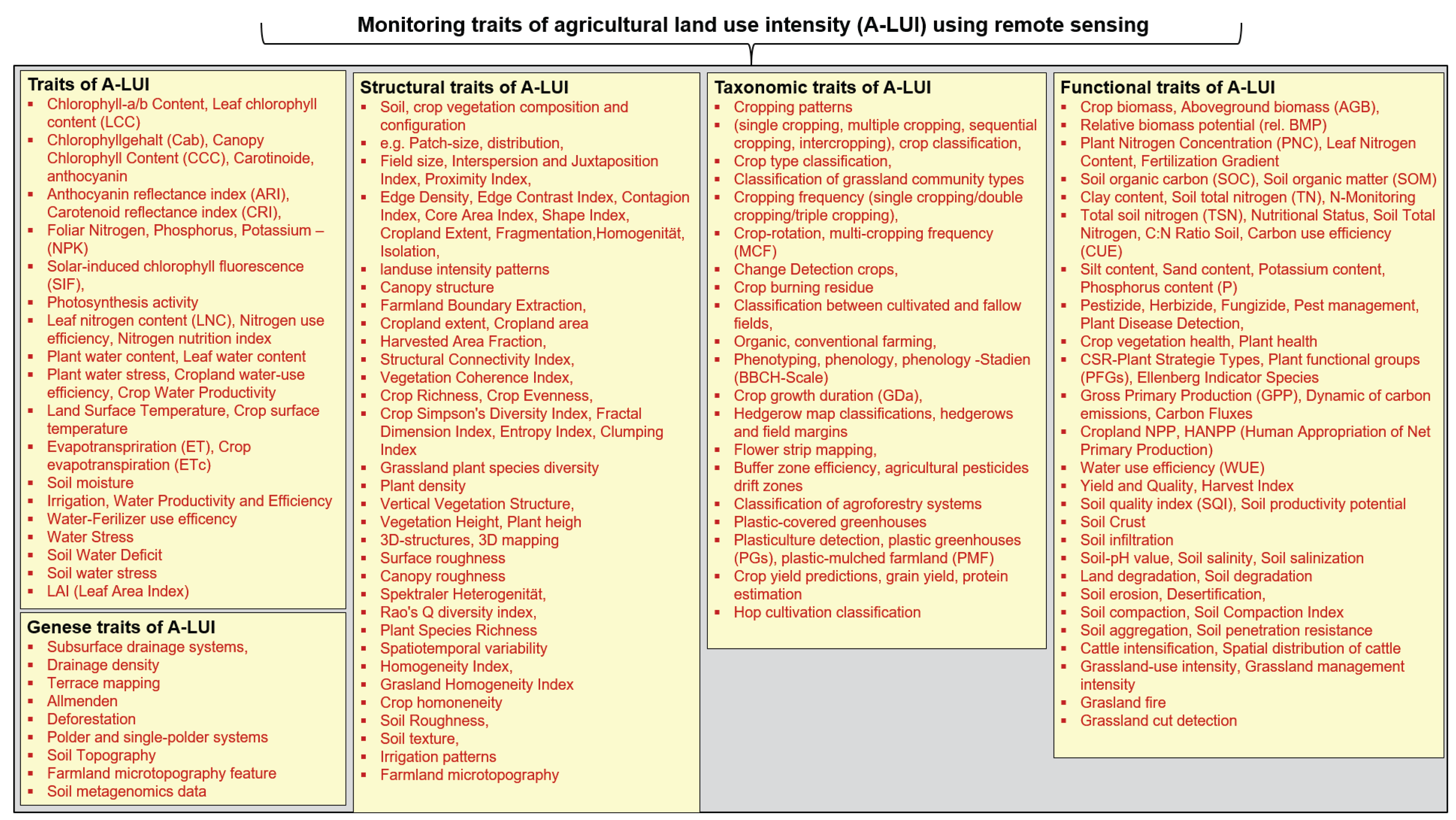

Table 1A.
Geographical area of monitoring, temporal availability of indicators, link, and selected examples of indicators for measuring and monitoring agricultural land use intensity; carried out by the FAO, OECD, World Bank and EUROSTAT.
Table 1A.
Geographical area of monitoring, temporal availability of indicators, link, and selected examples of indicators for measuring and monitoring agricultural land use intensity; carried out by the FAO, OECD, World Bank and EUROSTAT.
| FAO | OECD | World Bank | EUROSTAT | |
|---|---|---|---|---|
|
Geographical area of monitoring |
Worldwide coverage, with a special focus on developing countries | Primarily OECD member countries, focus on highly developed industrialised nations | Developing countries and emerging markets | European Union (EU) and some enlargement countries |
| Time availability of the indicators | Indicators of land use intensity have been available since the 1960s, Increased surveillance since the 1990s |
Data and analyses on land use intensity since the 1980s, Regular reports since the early 2000s. |
Data on land use intensity since the 1990s, Comprehensive database (WDI) since the 2000s. |
Harmonised data on agriculture and land use since the 1990s, Regular (every three to five years) surveys since the 1990s |
| Link | FAO database FAOSTAT https://www.fao.org/statistics/data-dissemination/agrifood-systems/en, (data access: 11.07.2024) |
OECD https://www.oecd.org/, (data access: 11.07.2024) |
World Development Indicators (WDI) https://databank.worldbank.org/source/world-development-, (data access: 11.07.2024) |
Farm Structure Surveys (FSS) https://ec.europa.eu/eurostat/web/microdata/farm-structure-survey (data access: 11/07/2024) |
| Indicators (selective examples) | ||||
| Indicator | FAO | OECD | World Bank | Eurostat |
| Agricultural area | Total area for agriculture (arable land, permanent grassland, permanent crops) | Agricultural land, including arable land, permanent crops, and pastures | Agricultural land (sq. km) | Utilised agricultural area (UAA) |
| Arable land | Land for crops, including repeatedly cultivated soils and fallow land | Arable land, including temporary crops and fallow land | Arable land (hectares) | Arable land |
| Permanent grassland | Land for perennial grasses and forage plants | Permanent pastures and meadows | Permanent meadows and pastures (hectares) | Permanent grassland |
| Permanent crops | Land for perennial crops such as fruit trees and vineyards | Permanent crops, such as orchards and vineyards | Permanent crops (hectares) | Permanent crops |
| Harvest yields | Amount of crop per unit area | Crop yields, measured by specific crop outputs per hectare | Cereal yield (kg per hectare) | Crop production per unit area |
| Use of fertilisers | Amount of fertiliser per hectare | Fertiliser consumption (kg per hectare of arable land) | Fertiliser consumption (kg per hectare of arable land) | Consumption of fertilisers per unit area of agricultural land |
| Pesticide use | Amount of pesticides per hectare | Pesticide sales and usage | Pesticide consumption (kg per hectare of arable land) | Pesticide sales and consumption |
| Irrigated area | Proportion of artificially irrigated agricultural land | Area equipped for irrigation (hectares) | Irrigated land (% of total agricultural land) | Irrigated area |
| Machine inventory | Number and type of machines per unit area | Agricultural machinery, such as tractors per hectare | Agricultural machinery (tractors per 100 sq. km of arable land) | Number of tractors and other agricultural machinery per unit area of agricultural land |
| Labour input | Labour hours per unit area | Labour input in agriculture, measured by hours worked per hectare | Employment in agriculture (% of total employment) | Labour force in agriculture |
| Livestock density | Number of animals per unit area of pastureland | Livestock density, measured as livestock units per hectare of pasture land | Livestock production index | Livestock density per unit area of pasture land |
| Carbon sequestration in the soil | Amount of carbon sequestered in the soil | Soil organic carbon content | Soil organic carbon content | Soil organic carbon content |
| Ground cover | Type and extent of ground cover | Land cover types and changes | Land cover (% of land area) | Land cover and land use |
| Erosion risk | Risk of soil erosion due to water or wind | Soil erosion rates | Soil erosion rates | Soil erosion and degradation risk |
| Biodiversity | Diversity of plant and animal species on farmland land (eg. Farmland birds, pollinators, butterflies) | Farmland biodiversity indices (eg. Farmland birds, pollinators, butterflies) | Agricultural biodiversity indices (eg. Farmland birds, pollinators, butterflies) | Biodiversity indicators in agricultural landscapes (eg. Farmland birds, pollinators, butterflies) |
| Water consumption in agriculture | Amount of water used for irrigation | Agricultural water withdrawal | Agricultural water withdrawal (% of total water withdrawal) | Water use in agriculture |
| Agricultural production per unit of input | Efficiency of the means of production in agriculture | Total factor productivity in agriculture | Agricultural value added per worker | Output per hectare of agricultural land |
| Energy consumption in agriculture | Energy consumption in agriculture | Energy use in agriculture | Energy use in agriculture | Energy consumption in agriculture |
| Sustainability indicators | Sustainability of agricultural practices | Sustainable agriculture practices indicators | Sustainable land management indicators | Sustainable farming practices |
| Climate impact of agriculture | Greenhouse gas emissions from agriculture | Greenhouse gas emissions from agriculture | Agricultural methane emissions (kt of CO2 equivalent) | Greenhouse gas emissions from agriculture |
| Nutrient balance in the soil | Balance of nitrogen and phosphorus in the soil | Nitrogen and phosphorus balance | Soil nutrient balance | Nutrient balance in agricultural soils |
| Bioproductivity | Productivity of biological systems on agricultural land | Biological productivity of agricultural systems | Agricultural productivity indexes | Biological productivity of agricultural lands |
| Plant protection measures | Measures to combat pests and diseases | Pest and disease control practices | Pest and disease control indicators | Plant protection measures and their impact |
| Energy efficiency in agriculture | Efficiency of energy consumption in agriculture | Energy efficiency in agricultural practices | Energy productivity in agriculture | Energy efficiency indicators in farming |
| Utilisation of genetic resources | Utilisation and conservation of genetic resources in agriculture | Use and conservation of genetic resources | Genetic resource management indicators | Conservation and use of agricultural genetic resources |
| Landscape diversity | Diversity of landscapes and agroecosystems | Landscape diversity and heterogeneity | Landscape diversity indicators | Landscape heterogeneity and diversity in agricultural areas |
| Soil compaction | Degree of soil compaction caused by agricultural machinery | Soil compaction indicators | Soil compaction risk | Soil compaction due to agricultural practices |
| Waste management in agriculture | Handling agricultural waste | Agricultural waste management practices | Waste management in agriculture | Management and recycling of agricultural waste |
| Soil moisture | Moisture content of the soil | Soil moisture levels | Soil moisture content indicators | Soil moisture monitoring in agricultural lands |
| Landscape fragmentation | Fragmentation of natural and agricultural landscapes | Landscape fragmentation and its impact on agriculture | Landscape fragmentation indexes | Impact of landscape fragmentation on agriculture |
| Sustainable land use practices | Spreading sustainable agricultural practices | Adoption of sustainable agricultural practices | Sustainable land management practices | Implementation of sustainable farming practices |
| Water utilisation efficiency | Efficiency of water utilisation in agriculture | Water use efficiency in agricultural practices | Agricultural water productivity | Water use efficiency in irrigated agriculture |
| Agroecological indicators | Indicators for the assessment of agroecological systems | Agro-ecological assessment indicators | Agro-ecological practices | Assessment of agro-ecological systems |
| Erosion due to wind | Loss of topsoil due to wind erosion | Wind erosion rates | Wind erosion indicators | Impact of wind erosion on agricultural land |
| Soil fertility | Level of soil fertility and its changes | Soil fertility levels | Soil fertility indicators | Changes in soil fertility |
| Land use changes | Changes in the utilisation of agricultural land | Changes in agricultural land use | Land use change indicators | Agricultural land use changes |
| Irrigation efficiency | Efficiency of irrigation methods | Irrigation efficiency | Efficiency of irrigation systems | Efficiency of water use in irrigation systems |
| Climate adaptation measures | Measures to adapt to climate change | Climate adaptation practices in agriculture | Climate resilience indicators | Implementation of climate adaptation measures in agriculture |
| Resource utilisation efficiency | Efficient use of natural resources | Resource use efficiency in agriculture | Resource productivity indicators | Efficiency of resource use in agriculture |
| Soil acidification | Degree of soil acidification and its causes | Soil acidification levels | Soil pH indicators | Impact of acidification on agricultural soils |
| Soil salinisation | Level of soil salinisation and its effects | Soil salinisation rates | Soil salinity indicators | Effects of salinisation on agricultural productivity |
| Utilisation of renewable energies | Share of renewable energies in agriculture | Renewable energy use in agricultural practices | Share of renewable energy in agriculture | Use of renewable energy sources in farming |
| Environmentally friendly cultivation methods | Spreading environmentally friendly cultivation methods | Adoption of eco-friendly farming practices | Eco-friendly agricultural practices | Implementation of environmentally friendly farming methods |
| Economic sustainability | Economic viability of farms | Economic sustainability of agricultural holdings | Economic viability indicators | Economic sustainability of farms |
| Social sustainability | Social aspects of agricultural practice | Social sustainability in agriculture | Social indicators in rural areas | Social impacts of agricultural practices |
| Productivity per unit area | Productivity of agricultural land | Land productivity indicators | Productivity of agricultural land | Output per unit of agricultural area |
| Water quality indicators | Impact of agriculture on water quality | Impact of agriculture on water quality | Water quality in agricultural areas | Effects of agricultural runoff on water quality |
| Infrastructure for agriculture | Availability and quality of agricultural infrastructure | Agricultural infrastructure development | Infrastructure investment in agriculture | Quality and accessibility of agricultural infrastructure |
| Innovation in agriculture | Implementation of new technologies and processes | Agricultural innovation and technology adoption | Innovation indicators in agriculture | Adoption of new agricultural techn |
Table A2.
High spatial resolution satellite missions, sensor/type, spatial resolution, spectral bands/type, availability, launch date and operator.
Table A2.
High spatial resolution satellite missions, sensor/type, spatial resolution, spectral bands/type, availability, launch date and operator.
| Satellit / Mission | Sensor / Typ | Spatial resolution | Spectral bands / Sensor typ | Availability | Start date |
Operator of the satellite mission |
|---|---|---|---|---|---|---|
| WorldView-3 | Visible (PAN+MS+SWIR) | 0,31 m (PAN), 1,24 m (MS) | Panchromatic Multispectral SWIR |
Commercial | 2014 | Maxar |
| WorldView-2 | Optically | 0,46 m (PAN), 1,84 m (MS) | Panchromatic Multispectral |
Commercial | 2009 | Maxar |
| GeoEye-1 | Optically | 0,41 m (PAN), 1,65 m (MS) | Panchromatic Multispectral |
Commercial | 2008 | Maxar |
| Pleiades Neo | Optically | 0,3 m (PAN), 1,2 m (MS) | Panchromatic Multispectral |
Commercial | 2021+ | Airbus |
| Pleiades 1A/1B | Optically | 0,5 m (PAN), 2,0 m (MS) | Panchromatic Multispectral |
Commercial | 2011/2012 | Airbus |
| SkySat | Optically + Video | 0,5–0,8 m (PAN), 1–2 m (MS) | RGB, NIR, Video | Commercial | 2013+ | Planet |
| BJ-3B (SuperView-2) | Optically | 0,3 m (PAN), 1,2 m (MS) | Panchromatic Multispectral |
Commercial | 2022 | 21AT (China) |
| Capella Space | RADAR (X-Band SAR) | 0,3–0,5 m (Spotlight) | SAR | Commercial | 2018+ | Capella Space (USA) |
| ICEYE | RADAR (X-Band SAR) | 0,25–1 m | SAR | Commercial | 2018+ | ICEYE (Finnland) |
| TerraSAR-X | RADAR (X-Band SAR) | bis 1 m (Spotlight-Modus) | SAR | Commercial / Scientifically free | 2007 | DLR / Airbus |
| PAZ | RADAR (SAR) | 1 m | SAR (X-Band) | Commercial | 2018 | Hisdesat (Spain) |
| Sentinel-1A/B | RADAR (C-Band SAR) | 10 m | SAR | Freely available | 2014/2016 | ESA / Copernicus |
| Drohnen / UAV | Optically + Multispectral | < 0,1 m | RGB, Multispectral, Hyperspectral, LiDAR |
Own operation | User-based | |
| Aerial photos | Optically | 0,20cm | Orthophotos (DOP) True Orthophotos, RGB, CIR |
Commercial / Authorities and partly scientific free | Federal states, Federal Agency for Cartography and Geodesy |
Here is a comprehensive table summarising the various indicators for measuring agricultural land use intensity and landscape structure that can be measured using RS:
Table A3.
Various indicators for measuring agricultural land use intensity that can be detected using RS. Here is a comprehensive table summarising the various indicators for measuring agricultural land use intensity and landscape structure that can be measured using RS:.
Table A3.
Various indicators for measuring agricultural land use intensity that can be detected using RS. Here is a comprehensive table summarising the various indicators for measuring agricultural land use intensity and landscape structure that can be measured using RS:.
| Indikator | Satelliten | Reference |
|---|---|---|
| Trait diversity of LUI | ||
| Chlorophyll-a/b Content Leaf chlorophyll content (LCC) Chlorophyllgehalt (Cab) Canopy Chlorophyll Content (CCC) Carotinoide, anthocyanin Anthocyanin reflectance index (ARI) Carotenoid reflectance index (CRI) |
Sentinel-11, Sentinel-21, Landsat 81, CRIME1, , EnMAP1, Airborne hyperspectral CASI2, Airborne Visible/ Infrared Imaging Spectrometer AVIRIS2, Airborne HyMap2, UAV-(HSP,MSP)3, Handheld portable hyperspectral camera (Specim IQ) ASD4, Laboratory spectroscopy5 |
[87,88,252,253,254,255,256,257,258,259,94,97,110,247,248,249,250,251] |
| Foliar Nitrogen, Phosphorus, Potassium - NPK | UAV (LiDAR, MSP) 3, SVC HR-1024i spectrometer ASD4 | [87,260,261] |
|
Solar-induced chlorophyll fluorescence (SIF), Photosynthesis activity |
Sentinel-31, GOSIF data1, AS-SpecFOM (Ground based)6, FluoSpec2 system (Ground based) | [72,99,262,263,264,265] |
| Leaf nitrogen content (LNC) Nitrogen use efficiency, Nitrogen nutrition index |
Sentinel-21, CRIME1, PRISMA1,Airborne micro-hyperspec NIR-100 camera2, UAV | [87,88,90,111,112,266,267] |
| Plant water content Leaf water content Plant water stress Cropland water-use efficiency Crop Water Productivity |
GLASS1, Landsat1, Sentinel-21, UAV (MSP, HSP)3, mmWave RADAR (Tower)6, Cropland ecosystem flux sites6, Local TIR Sensor6, |
[268,269,270,271,272,273,274,275,276] |
| Land Surface Temperature Crop surface temperature |
Landsat1, High Spatio-Temporal Resolution Land Surface Temperature Monitoring (LSTM) Mission1, UAV (TIR, RGB, MSP)3 |
[272,277,278,279,280,281] |
| Evapotranspriration (ET) Crop evapotranspiration (ETc) |
MODIS1, DEIMOS-1 is a commercial tasking EO satellit1, Landsat1, Sentinel-21, SuperDove satellites (PlanetScope)1, UAV-(RGB, MSP, TIR)3 | [282,283,284,285,286,287,288,289,290] |
| Soil moisture | MODIS-Terra1, Landsat1,AMSR-21,AMSR-E1, NISAR1, Sentinel-11, Sentinel-21, SMAP1, Airborne hyperspectral (DAIS)2, Airborne hyperspectral (AISA Eagle, Hawk) 2 | [291,292,293,294,295,296,297,298,299] |
| Irrigation Irrigation Efficiency Water Productivity and Efficiency Irrigation patterns Water-Ferilizer use efficency Water Stress Soil Water Deficit Soil water stress |
MODIS1, Landsat1, Sentinel-21, UAV (MSP)3, ASD4, |
[300,301,310,311,302,303,304,305,306,307,308,309] |
| LAI (Leaf Area Index) | MODIS1, Landsat1, Sentinel-21, UAV-(HSP, TIR, LiDAR)3, Ocean Optics USB2000 (Tower)6 | [255,256,312,313,314] |
| Genese Trait Diversity of LUI | ||
| Subsurface drainage systems, Drainage density |
RADAR (SAR)1, Landsat1, Senitnel-21, Airborne LiDAR2, Airborne data2, UAV – RGB, CIR, TIR3 | [124,125,126,127,128,315,316] |
| Terrace mapping | Landsat1, Sentinel-11, Sentinel-21, GF-2 satellite image1, WorldView-11, WorldView-31, Airborne LiDAR2, UAV-LiDAR3 | [129,130,131,136,137,138] |
| Allmenden | Airborne LiDAR3 | [139,140] |
| Deforestation | MODIS1, ALOS PALSAR data1, RADARSAT-21, Landsat1, Sentinel-11, Sentinel-21, UAV (RGB, NIR, IRT)3 | [143,144,145,146,147,317,318,319,320] |
| Polder and single-polder systems | Google Earth RS data1, Corona spy satellite imagery1 | [321,322] |
| DEM (Digital Elevation Model) DSM (Digital Surface Model) |
SRTM1, TerraSAR-X1, TanDEM-X1, Sentinel-11, Sentinel-31, ALOS-2 PALSAR-21, ALOS PRISM1, Terra ASTER1, ICESat GLAS1, Airborne LiDAR2, UAV (SAR, RGB)3 | [61,323,332,333,334,335,324,325,326,327,328,329,330,331] |
| Soil Topography Farmland microtopography feature |
Landsat1, Sentinel-11, Sentinel-21, CORONA KH-4B1, Gaofen-7 satellite1, Airborne LiDAR2 | [166,336,337,338,339,340] |
| Soil metagenomics data | UAV (MSP, LiDAR)3 | [341] |
| Structural traits of LUI | ||
| Soil, crop vegetation composition and configuration (e.g. Patch-size, distribution Field size, Interspersion and Juxtaposition Index, Proximity Index, Edge Density, Edge Contrast Index, Contagion Index, Core Area Index, Shape Index, Cropland Extent, Fragmentation,Homogenity, Isolation, Landuse intensity patterns, Canopy structure Farmland Boundary Extraction, Cropland extent, Cropland area, Harvested Area Fraction, Structural Connectivity Index, Vegetation Coherence Index, Crop Richness, Crop Evenness, Crop Simpson's Diversity Index, Fractal Dimension Index, Entropy Index, Clumping Index, Grassland plant species diversity Plant density |
MODIS1, Landsat1, Spot1, Sentinel-21, WorldView-2/-31, QuickBird1, Pleiades1, GeoEye1, GF-21, RapidEye1, PlanetScope1, Airborne Hyperspectral AVIRIS and HYDICE2, Airborne data2, UAV (RGB, MSP, HSP)3 | [31,33,344,345,346,347,348,349,350,351,352,353,67,354,355,356,148,149,156,157,266,342,343] |
| Vertical Vegetation Structure, Vegetation Height, Plant heigh 3D-structures, 3D mapping |
GEDI LiDAR1, ICESat-21, UAV (RGB, LiDAR) Phenotyping robot “MARS-PhenoBot”6, 6-DOT robot6, RGB-Camera6, Terrestrial LiDAR6 |
[357,358,359,360,361,362] |
| Surface roughness Cnopy roughness |
Sentinel-11, MODIS1, UAV (RGB)3 | [162,163,164] |
| Spektraler Heterogenität, Rao's Q diversity index, Plant Species Richness Spatiotemporal variability |
MODIS1, Landsat1, Sentinel-21 | [160,161,363] |
| Homogeneity Index, Grasland Homogeneity Index Crop homoneneity |
Sentinel-11, Sentinel-21, GF-21 | [364,365,366] |
| Soil Roughness, Soil texture, Farmland microtopography |
Landsat1, Sentinel-11, Sentinel-21, AHSI/ZY1-02D satellite1, SRTM1, Airborne LiDAR2, ASD Handspectometer4, Smartphone-captured digital images6 | [166,167,374,375,340,367,368,369,370,371,372,373] |
| Taxonomic LUI | ||
| Cropping patterns (single cropping, multiple cropping, sequential cropping, intercropping) |
MODIS1, Spot1, Landsat1, Sentinel-11, Sentinel 21, IRS1, WiFS1, Airborne AVIRIS2, RADARSAT-21, Airborne LiDAR2 | [150,168,177,178,181,376,377,169,170,171,172,173,174,175,176] |
| Crop classification, Crop type classification Crop type mapping |
MODIS1, Landsat1, Sentinel-11, Sentinel-21, Sentinel-31, Airborne AVIRIS2, UAV (HSP)3 | [135,151,182,378,379,380,381,382,383,384] |
| Classification of grassland community types | Landsat1, Sentinel-11, Sentinel-21 | [385,386,387] |
| Cropping frequency (single cropping/double cropping/triple cropping) Crop-rotation Multi-cropping frequency (MCF) Croping intensity Cropping intensity index Change Detection crops |
MODIS1, Gaofen-11, GF-11, Landsat1, Sentinel-11, Sentinel-21 | [169,183,394,395,396,397,349,377,388,389,390,391,392,393] |
| Crop residue cover mapping | Landsat1, Sentinel-21, Google Earth Engine1, UAV3, FieldSpec Pro4, Photo analysis surveys6 |
[398,399,400,401,402,403] |
| Crop burning residue | MODIS1, AVHRR1, LISS-III1, LISS-IV1, UAV3 | [404,405,406] |
| Classification between cultivated and fallow fields |
MODIS1, Landsat1, Sentinel-21 | [376,388,407,408,409] |
| Organic, conventional farming Organic and non-organic farming |
Landsat1, Spot1, Sentinel-21, KOMPSAT-21, WorldView-21, UAV (RGB)3, Hyperspectral ASD4 | [410,411,412,413] |
| Phenotyping, Phenology, Phenology-Stadien (BBCH-Scale) |
UAV (RGB, MSP, HSP, TIR, LiDAR)3, UAV (RGB, VIS, NIR, TIR, LiDAR)3, Labor-Hyperspectral – AISA-EAGLE5 | [252,312,335,414,415,416,417,418,419] |
| Crop growth duration (GDa), | MODIS1, Landsat1, Gaofen-11, Sentinel-21, RapidEye1, UAV (SAR)2 | [394,420,421,422,423] |
| Hedgerow map classifications, Hedgerows and field margins |
TerraSAR-X1, Spot1, IKONOS1, Airborne MSP2, Aerial photographs2, UAV (RGB, MSP)3 | [424,425,426,427,428,429] |
| Flower strip mapping Flower Mapping |
Airborne Hyperspectral (HySPEX, RGB, TIR)2, Airborne Hyperspectral (AISA-Eagle)2, Airborne MSP2, UAV (MSP, HSP)3 | [429,430,431,432,433,434] |
| Buffer Zone Efficiency Agricultural Pesticides Drift zones |
Landsat1, Sentinel-21 | [435] |
| Classification of agroforestry systems | RapidEye1, PlantetScope1, LISS IV1, Sentinel-21 | [436,437,438,439,440] |
| Plastic-covered greenhouses Plasticulture detection Plastic greenhouses (PGs) and Plastic-mulched farmland (PMF) |
Landsat1, Sentinel-11, Sentinel-21, GF-2 | [441,442,443,444,445] |
| Crop yield predictions Grain Yield, Protein estimation |
MODIS1, Landsat1, Sentinel-21, UAV – (MSP, HSP)3 | [266,446,455,447,448,449,450,451,452,453,454] |
| Hop cultivation classification | UAV (MSP)3, Mobile phone camera6 | [456,457] |
| Functional traits of LUI | ||
| Crop biomass, Aboveground biomass (AGB), Relative biomass potential (rel. BMP) |
MODIS1, Landsat1, Sentinel-11, Sentinel-21, PlanetScope1, UAV (MSP, RGB)3, Smartphone6 | [188,189,190,191,192,193,194,301,458] |
|
Plant Nitrogen Concentration (PNC) Leaf Nitrogen Content Fertilization Gradient |
Sentinel-21, UAV (MSP, TIR)3 | [94,203,204,205,459,460,461] |
| Soil organic carbon (SOC) Soil organic matter (SOM) |
ALOS-21, PALSAR-21, Landsat1, Spot 4/51, GF-11, RADAR (PLAS)1, Sentinel-11, Sentinel-21, Sentinel-31, Airborne hyperspectral (DAIS)2, Airborne hyperspectral (AISA Eagle, Hawk)2, Hyperspectral APEX2, UAV (SAR)3, VIS–NIR spectroscopy (Field)1, | [208,213,465,466,467,468,469,470,471,472,473,474,214,219,221,222,299,462,463,464] |
| Clay content | Landsat1, Aster1, Sentinel-21, Airborne hyperspectral (AISA Eagle, Hawk)2 | [375,475,476,477,478,479,480,481] |
| Soil total nitrogen (TN) N-Monitoring Total soil nitrogen (TSN) Nutritional Status Soil Total Nitrogen Soil Nutrients Contents |
Sentinel-11, Sentinel-21, GF-11, UAV (HSP, MSP, TIR)3, ASD (Field)4 | [206,213,488,469,480,482,483,484,485,486,487] |
| C:N Ratio Soil | Landsat1, Sentinel-11, Sentinel-21, Sentinel-31 | [222,468,489,490,491,492] |
| Carbon use efficiency (CUE) | MODIS1, Landsat1, Sentinel-21 | [493,494,495,496] |
| Silt content | GF-11, Airborne hyperspectral (AISA Eagle, Hawk)2, | [375,497] |
| Sand content | Landsat1, Sentinel-21, Aster1, GF-11, Planet/NICFI1, Airborne hyperspectral (AISA Eagle, Hawk)2 | [375,481,497,498,499,500,501] |
| Potassium content | PRISMA1, UAV (MSP)3 | [484,485] |
| Phosphorus content (P) | MODIS1, Landsat1, Sentinel-21, PRISMA1, UAV (MSP, LiDAR)3, ASD4 | [341,484,485,486,487,502] |
|
Pestizide, Herbizide, Fungizide Pest management |
Sentinel-21, UAV3, Local hyperspectral camera6, ASD - LeafSpec hyperspectral images4 | [195,196,197,198,199,200,503,504] |
| Plant Disease Detection, Crop vegetation health Plant health |
Sentinel-11, Sentinel-21, UAV (RGB, MSP, VIS, NIR, TIR, LiDAR)3, ASD FieldSpec Pro FR4 | [97,202,511,512,513,514,515,516,411,416,505,506,507,508,509,510] |
| CSR-Plant Strategie Types Plant functional groups (PFGs) Ellenberg Indicator Species |
Landsat1, Sentinel-21, Airborne hyperspectral data (AISA dual)2, Airborne AISA Fenix2, Airborne imaging spectrometer APEX2, Airborne hyperspectral HySpex2 | [517,518,519,520,521,522,523,524] |
| Gross Primary Production (GPP) Dynamic of carbon emissions, Carbon Fluxes |
MODIS1, Meris1, Landsat1, Sentinel-11, Sentinel-21, Sentinel-31, Hyperspectral Ocean Optics USB2000 (Tower)6, LEDAPS-Aerosol Robotic Network (AERONET)6 | [254,493,525,526,527,528,529,530,531,532] |
| Cropland NPP | MODIS1, Landsat1, UAV (MSP)3 | [149,314,493,533,534,535,536,537,538] |
| HANPP (Human Appropriation of Net Primary Production) | MODIS1, Landsat1, Sentinel-21 | [539,540,541,542,543] |
| Water use efficiency (WUE) | MODIS1, Landsat1, Sentinel-11, Sentinel-21 | [493,544,545,546,547,548] |
| Yield and Quality | Landsat1, Sentinel-11, Sentinel-21, UAV (MSP)3 | [193,531,549,550,551,552,553,554,555,556] |
| Harvest Index | MODIS1, HJ-1 satellite1, Sentinel-21, UAV (HSP)3, FieldSpec HandHeld Spectroradiometer (ASD)4 | [557,558,559,560] |
| Soil quality index (SQI) | Landsat1, Sentinel-21, Airborne hyperspectral (AISA)2 | [338,561,562] |
| Soil productivity potential | MODIS1, Landsat1, Sentinel-21, ASD FieldSpec4 | [310,480,563,564,565] |
| Soil Crust | KOMPSAT-2 satellite1, Airborne hyperspectral (DAIS)2, Airborne hyperspectral (AISA Eagle, Hawk)2, UAV (RGB, MSP, HSP)3, ASD Fieldspec4 | [299,566,567,568,569,570,571,572] |
| Soil infiltration | Airborne hyperspectral (DAIS)2, Airborne hyperspectral (AISA Eagle, Hawk)2, Airborne CASI-15002, SASI-6002, Airborne TASI-600 hyperspectral sensors2, UAV (HSP, Cubert UHD-185)3 | [299,573,574] |
| Soil-pH value | PALSAR-1/21, SRTM1, Landsat1, PlantetScope1, Sentinel-11, Sentinel-21, UAV (MSP)3, ASD FieldSpec4 | [298,368,582,583,584,585,555,575,576,577,578,579,580,581] |
| Soil salinity Soil salinization |
Landsat1, RADAR1, Airborne LiDAR2, HJ-1 Hyperspectral Imager Data2 | [298,586,587,588,589,590,591,592,593] |
| Land degradation, Soil degradation, Soil erosion Desertification |
Landsat1, SRTM1, Sentinel-11, Sentinel-21, RapidEye1, Airborne hyperspectral (DAIS)2, Airborne hyperspectral (AISA Eagle, Hawk)2, UAV (RGB)3 | [299,594,595,596,597,598,599] |
| Soil compaction Soil Compaction Index Soil aggregation Soil penetration resistance |
Landsat1, GoogleEarth aerial imagery1, Sentinel-21, RapidEye1, Airborne hyperspectral (CASI)2, UAV (RGB, SAR, LiDAR, MSP, TIR)3 | [595,600,601,602,603,604,605,606,607] |
| Cattle intensification, Spatial distribution of cattle |
Sentinel-11, Sentinel-21 | [608] |
| Grassland-use intensity Grassland management intensity |
Landsat1, Sentinel-11, Sentinel-21, RapidEye1, | [184,187,609,610,611,612,613] |
| Grasland fire | MODIS1, Sentinel-11, Sentinel-21, GF-6 WFV1, UAV3 | [614,615,616,617,618] |
| Grassland cut detection | SAR1, Sentinel-11, Sentinel-21 | [619,620,621] |
| Different Water quality indicators | All RS Sensors with all RS characteristics (MSP, HSP, TIR, RADAR, LiDAR) | [63] |
The sensor is used on the RS platform: 1 - spaceborne RS platforms, 2 - airborne RS platform, 3-UAV, 4- Handheld portable hyperspectral camera (Specim IQ) ASD, 5-Laboratory spectroscopy, 6-Tower, Smartphone, Ground based.
References
- Diogo, V.; Helfenstein, J.; Mohr, F.; Varghese, V.; Debonne, N.; Levers, C.; Swart, R.; Sonderegger, G.; Nemecek, T.; Schader, C.; et al. Developing context-specific frameworks for integrated sustainability assessment of agricultural intensity change: An application for Europe. Environ. Sci. Policy 2022, 137, 128–142. [CrossRef]
- Tripathi, S.; Srivastava, P.; Devi, R.S.; Bhadouria, R. Influence of synthetic fertilizers and pesticides on soil health and soil microbiology. In Agrochemicals Detection, Treatment and Remediation; Elsevier, 2020; pp. 25–54.
- YAHAYA, S.M.; MAHMUD, A.A.; ABDULLAHI, M.; HARUNA, A. Recent advances in the chemistry of nitrogen, phosphorus and potassium as fertilizers in soil: A review. Pedosphere 2023, 33, 385–406. [CrossRef]
- Shah, A.N.; Tanveer, M.; Shahzad, B.; Yang, G.; Fahad, S.; Ali, S.; Bukhari, M.A.; Tung, S.A.; Hafeez, A.; Souliyanonh, B. Soil compaction effects on soil health and cropproductivity: an overview. Environ. Sci. Pollut. Res. 2017, 24, 10056–10067. [CrossRef]
- Ingrao, C.; Strippoli, R.; Lagioia, G.; Huisingh, D. Water scarcity in agriculture: An overview of causes, impacts and approaches for reducing the risks. Heliyon 2023, 9, e18507. [CrossRef]
- Scanlon, B.R.; Jolly, I.; Sophocleous, M.; Zhang, L. Global impacts of conversions from natural to agricultural ecosystems on water resources: Quantity versus quality. Water Resour. Res. 2007, 43. [CrossRef]
- Sharma, K.; Rajan, S.; Nayak, S.K. Water pollution: Primary sources and associated human health hazards with special emphasis on rural areas. In Water Resources Management for Rural Development; Elsevier, 2024; pp. 3–14.
- Pannard, A.; Souchu, P.; Chauvin, C.; Delabuis, M.; Gascuel-Odoux, C.; Jeppesen, E.; Le Moal, M.; Ménesguen, A.; Pinay, G.; Rabalais, N.N.; et al. Why are there so many definitions of eutrophication? Ecol. Monogr. 2024, 1–25. [CrossRef]
- Zabel, F.; Delzeit, R.; Schneider, J.M.; Seppelt, R.; Mauser, W.; Václavík, T. Global impacts of future cropland expansion and intensification on agricultural markets and biodiversity. Nat. Commun. 2019, 10, 1–10. [CrossRef]
- Mupepele, A.C.; Bruelheide, H.; Brühl, C.; Dauber, J.; Fenske, M.; Freibauer, A.; Gerowitt, B.; Krüß, A.; Lakner, S.; Plieninger, T.; et al. Biodiversity in European agricultural landscapes: transformative societal changes needed. Trends Ecol. Evol. 2021, 36, 1067–1070. [CrossRef]
- Burian, A.; Kremen, C.; Wu, J.S.T.; Beckmann, M.; Bulling, M.; Garibaldi, L.A.; Krisztin, T.; Mehrabi, Z.; Ramankutty, N.; Seppelt, R. Biodiversity–production feedback effects lead to intensification traps in agricultural landscapes. Nat. Ecol. Evol. 2024, 8, 752–760. [CrossRef]
- Le Provost, G.; Thiele, J.; Westphal, C.; Penone, C.; Allan, E.; Neyret, M.; van der Plas, F.; Ayasse, M.; Bardgett, R.D.; Birkhofer, K.; et al. Contrasting responses of above- and belowground diversity to multiple components of land-use intensity. Nat. Commun. 2021, 12, 3918. [CrossRef]
- Beckmann, M.; Gerstner, K.; Akin-Fajiye, M.; Ceaușu, S.; Kambach, S.; Kinlock, N.L.; Phillips, H.R.P.; Verhagen, W.; Gurevitch, J.; Klotz, S.; et al. Conventional land-use intensification reduces species richness and increases production: A global meta-analysis. Glob. Chang. Biol. 2019, 25, 1941–1956. [CrossRef]
- Felipe-Lucia, M.R.; Soliveres, S.; Penone, C.; Fischer, M.; Ammer, C.; Boch, S.; Boeddinghaus, R.S.; Bonkowski, M.; Buscot, F.; Fiore-Donno, A.M.; et al. Land-use intensity alters networks between biodiversity, ecosystem functions, and services. Proc. Natl. Acad. Sci. 2020, 117, 28140–28149. [CrossRef]
- Gossner, M.M.; Lewinsohn, T.M.; Kahl, T.; Grassein, F.; Boch, S.; Prati, D.; Birkhofer, K.; Renner, S.C.; Sikorski, J.; Wubet, T.; et al. Land-use intensification causes multitrophic homogenization of grassland communities. Nature 2016. [CrossRef]
- Millard, J.; Outhwaite, C.L.; Kinnersley, R.; Freeman, R.; Gregory, R.D.; Adedoja, O.; Gavini, S.; Kioko, E.; Kuhlmann, M.; Ollerton, J.; et al. Global effects of land-use intensity on local pollinator biodiversity. Nat. Commun. 2021, 12, 2902. [CrossRef]
- Suarez, A.; Gwozdz, W. On the relation between monocultures and ecosystem services in the Global South: A review. Biol. Conserv. 2023, 278, 109870. [CrossRef]
- Cheng, C.; Liu, Z.; Song, W.; Chen, X.; Zhang, Z.; Li, B.; van Kleunen, M.; Wu, J. Biodiversity increases resistance of grasslands against plant invasions under multiple environmental changes. Nat. Commun. 2024, 15, 1–10. [CrossRef]
- Scanes, C.G. Human Activity and Habitat Loss: Destruction, Fragmentation, and Degradation. In Animals and Human Society; Elsevier, 2018; pp. 451–482 ISBN 9780128052471.
- Oliver, T.H.; Marshall, H.H.; Morecroft, M.D.; Brereton, T.; Prudhomme, C.; Huntingford, C. Interacting effects of climate change and habitat fragmentation on drought-sensitive butterflies. Nat. Clim. Chang. 2015, 5, 941–946. [CrossRef]
- Peters, M.K.; Hemp, A.; Appelhans, T.; Becker, J.N.; Behler, C.; Classen, A.; Detsch, F.; Ensslin, A.; Ferger, S.W.; Frederiksen, S.B.; et al. Climate–land-use interactions shape tropical mountain biodiversity and ecosystem functions. Nature 2019, 568, 88–92. [CrossRef]
- Schneider, J.M.; Delzeit, R.; Neumann, C.; Heimann, T.; Seppelt, R.; Schuenemann, F.; Söder, M.; Mauser, W.; Zabel, F. Effects of profit-driven cropland expansion and conservation policies. Nat. Sustain. 2024. [CrossRef]
- Kaur, R.; Choudhary, D.; Bali, S.; Bandral, S.S.; Singh, V.; Ahmad, M.A.; Rani, N.; Singh, T.G.; Chandrasekaran, B. Pesticides: An alarming detrimental to health and environment. Sci. Total Environ. 2024, 915, 170113. [CrossRef]
- Bava, R.; Castagna, F.; Lupia, C.; Poerio, G.; Liguori, G.; Lombardi, R.; Naturale, M.D.; Mercuri, C.; Bulotta, R.M.; Britti, D.; et al. Antimicrobial Resistance in Livestock: A Serious Threat to Public Health. Antibiotics 2024, 13. [CrossRef]
- Khmaissa, M.; Zouari-Mechichi, H.; Sciara, G.; Record, E.; Mechichi, T. Pollution from livestock farming antibiotics an emerging environmental and human health concern: A review. J. Hazard. Mater. Adv. 2024, 13. [CrossRef]
- Turner, B.L.; Doolittle, W.E. THE CONCEPT AND MEASURE OF AGRICULTURAL INTENSITY. Prof. Geogr. 1978, 30, 297–301. [CrossRef]
- Herzog, F.; Steiner, B.; Bailey, D.; Baudry, J.; Billeter, R.; Bukácek, R.; De Blust, G.; De Cock, R.; Dirksen, J.; Dormann, C.F.; et al. Assessing the intensity of temperate European agriculture at the landscape scale. Eur. J. Agron. 2006, 24, 165–181. [CrossRef]
- Lüscher, G.; Jeanneret, P.; Schneider, M.K.; Turnbull, L.A.; Arndorfer, M.; Balázs, K.; Báldi, A.; Bailey, D.; Bernhardt, K.G.; Choisis, J.P.; et al. Responses of plants, earthworms, spiders and bees to geographic location, agricultural management and surrounding landscape in European arable fields. Agric. Ecosyst. Environ. 2014, 186, 124–134. [CrossRef]
- Helfenstein, J.; Hepner, S.; Kreuzer, A.; Achermann, G.; Williams, T.; Bürgi, M.; Debonne, N.; Dimopoulos, T.; Diogo, V.; Fjellstad, W.; et al. Divergent agricultural development pathways across farm and landscape scales in Europe: Implications for sustainability and farmer satisfaction. Glob. Environ. Chang. 2024, 86, 102855. [CrossRef]
- Canisius, F.; Turral, H.; Molden, D. Fourier analysis of historical NOAA time series data to estimate bimodal agriculture. Int. J. Remote Sens. 2007, 28, 5503–5522. [CrossRef]
- Kuemmerle, T.; Hostert, P.; St-Louis, V.; Radeloff, V.C. Using image texture to map farmland field size: A case study in Eastern Europe. J. Land Use Sci. 2009, 4, 85–107. [CrossRef]
- Verburg, P.H.; Neumann, K.; Nol, L. Challenges in using land use and land cover data for global change studies. Glob. Chang. Biol. 2011, 17, 974–989. [CrossRef]
- Kuemmerle, T.; Erb, K.; Meyfroidt, P.; Müller, D.; Verburg, P.H.; Estel, S.; Haberl, H.; Hostert, P.; Jepsen, M.R.; Kastner, T.; et al. Challenges and opportunities in mapping land use intensity globally. Curr. Opin. Environ. Sustain. 2013, 5, 484–493. [CrossRef]
- Wellmann, T.; Haase, D.; Knapp, S.; Salbach, C.; Selsam, P.; Lausch, A. Urban land use intensity assessment: The potential of spatio-temporal spectral traits with remote sensing. Ecol. Indic. 2018, 85, 190–203. [CrossRef]
- Weber, D.; Schwieder, M.; Ritter, L.; Koch, T.; Psomas, A.; Huber, N.; Ginzler, C.; Boch, S. Grassland-use intensity maps for Switzerland based on satellite time series: Challenges and opportunities for ecological applications. Remote Sens. Ecol. Conserv. 2024, 10, 312–327. [CrossRef]
- Liu, H.; Zhou, Z.; Wen, Q.; Chen, J.; Kojima, S. Spatiotemporal Land Use/Land Cover Changes and Impact on Urban Thermal Environments: Analyzing Cool Island Intensity Variations. Sustain. 2024, 16. [CrossRef]
- Qiu, B.; Liu, B.; Tang, Z.; Dong, J.; Xu, W.; Liang, J.; Chen, N.; Chen, J.; Wang, L.; Zhang, C.; et al. National-scale 10-m maps of cropland use intensity in China during 2018-2023. Sci. data 2024, 11, 691. [CrossRef]
- Hank, T.B.; Berger, K.; Bach, H.; Clevers, J.G.P.W.; Gitelson, A.; Zarco-Tejada, P.; Mauser, W. Spaceborne Imaging Spectroscopy for Sustainable Agriculture: Contributions and Challenges; Springer Netherlands, 2019; Vol. 40; ISBN 0123456789.
- Wulder, M.A.; Coops, N.C. Make Earth observations open access. Nature 2014, 513, 30–31. [CrossRef]
- Wulder, M.A.; Roy, D.P.; Radeloff, V.C.; Loveland, T.R.; Anderson, M.C.; Johnson, D.M.; Healey, S.; Zhu, Z.; Scambos, T.A.; Pahlevan, N.; et al. Fifty years of Landsat science and impacts. Remote Sens. Environ. 2022, 280, 113195. [CrossRef]
- Malenovský, Z.; Rott, H.; Cihlar, J.; Schaepman, M.E.; García-Santos, G.; Fernandes, R.; Berger, M. Sentinels for science: Potential of Sentinel-1, -2, and -3 missions for scientific observations of ocean, cryosphere, and land. Remote Sens. Environ. 2012, 120, 91–101. [CrossRef]
- Guanter, L.; Kaufmann, H.; Segl, K.; Foerster, S.; Rogass, C.; Chabrillat, S.; Kuester, T.; Hollstein, A.; Rossner, G.; Chlebek, C.; et al. The EnMAP Spaceborne Imaging Spectroscopy Mission for Earth Observation. Remote Sens. 2015, 7, 8830–8857. [CrossRef]
- Nieke, J.; Rast, M. Towards the Copernicus Hyperspectral Imaging Mission For The Environment (CHIME). In Proceedings of the IGARSS 2018 - 2018 IEEE International Geoscience and Remote Sensing Symposium; IEEE, 2018; pp. 157–159.
- Dubayah, R.; Blair, J.B.; Goetz, S.; Fatoyinbo, L.; Hansen, M.; Healey, S.; Hofton, M.; Hurtt, G.; Kellner, J.; Luthcke, S.; et al. The Global Ecosystem Dynamics Investigation: High-resolution laser ranging of the Earth’s forests and topography. Sci. Remote Sens. 2020, 1, 100002.
- Lee, C.M.; Cable, M.L.; Hook, S.J.; Green, R.O.; Ustin, S.L.; Mandl, D.J.; Middleton, E.M. An introduction to the NASA Hyperspectral InfraRed Imager (HyspIRI) mission and preparatory activities. Remote Sens. Environ. 2015, 167, 6–19.
- Kraft, S.; Del Bello, U.; Bouvet, M.; Drusch, M.; Moreno, J. FLEX: ESA’s Earth Explorer 8 candidate mission. Int. Geosci. Remote Sens. Symp. 2012, 7125–7128.
- Omia, E.; Bae, H.; Park, E.; Kim, M.S.; Baek, I.; Kabenge, I.; Cho, B.K. Remote Sensing in Field Crop Monitoring: A Comprehensive Review of Sensor Systems, Data Analyses and Recent Advances. Remote Sens. 2023, 15. [CrossRef]
- Sethy, P.K.; Pandey, C.; Sahu, Y.K.; Behera, S.K. Hyperspectral imagery applications for precision agriculture - a systemic survey; Springer US, 2022; Vol. 81; ISBN 0123456789.
- Maes, W.H.; Steppe, K. Perspectives for Remote Sensing with Unmanned Aerial Vehicles in Precision Agriculture. Trends Plant Sci. 2019, 24, 152–164. [CrossRef]
- Khanal, S.; Fulton, J.; Shearer, S. An overview of current and potential applications of thermal remote sensing in precision agriculture. Comput. Electron. Agric. 2017, 139, 22–32. [CrossRef]
- Segarra, J.; Buchaillot, M.L.; Araus, J.L.; Kefauver, S.C. Remote Sensing for Precision Agriculture: Sentinel-2 Improved Features and Applications. Agronomy 2020, 10, 641. [CrossRef]
- Barbosa Júnior, M.R.; Moreira, B.R. de A.; Carreira, V. dos S.; Brito Filho, A.L. de; Trentin, C.; Souza, F.L.P. de; Tedesco, D.; Setiyono, T.; Flores, J.P.; Ampatzidis, Y.; et al. Precision agriculture in the United States: A comprehensive meta-review inspiring further research, innovation, and adoption. Comput. Electron. Agric. 2024, 221, 108993. [CrossRef]
- Marques, P.; Pádua, L.; Sousa, J.J.; Fernandes-Silva, A. Advancements in Remote Sensing Imagery Applications for Precision Management in Olive Growing: A Systematic Review. Remote Sens. 2024, 16, 1324. [CrossRef]
- Bonfanti, J.; Langridge, J.; Avadí Ef, A.; Casajus, N.; Chaudhary, A.; Damour Hi, G.; Estrada-Carmona, N.; Jones, S.K.; Makowski, D.; Mitchell, M.; et al. Global review of meta-analyses reveals key data gaps in agricultural impact studies on biodiversity in croplands. BioRxiv 2024, 0–22.
- Khanal, S.; Kushal, K.C.; Fulton, J.P.; Shearer, S.; Ozkan, E. Remote sensing in agriculture—accomplishments, limitations, and opportunities. Remote Sens. 2020, 12, 1–29.
- Lu, B.; Dao, P.D.; Liu, J.; He, Y.; Shang, J. Recent advances of hyperspectral imaging technology and applications in agriculture. Remote Sens. 2020, 12, 1–44. [CrossRef]
- Lausch, A.; Selsam, P.; Pause, M.; Bumberger, J. Monitoring vegetation- and geodiversity with remote sensing and traits. Philos. Trans. R. Soc. A Math. Phys. Eng. Sci. 2024, 382. [CrossRef]
- Cavender-Bares, J.; Gamon, J.A.; Townsend, P.A. Remote Sensing of Plant Biodiversity; Cavender-Bares, J., Gamon, J.A., Townsend, P.A., Eds.; Springer International Publishing: Cham, 2020; ISBN 978-3-030-33156-6.
- Lausch, A.; Bastian, O.; Klotz, S.; Leitão, P.J.; Jung, A.; Rocchini, D.; Schaepman, M.E.; Skidmore, A.K.; Tischendorf, L.; Knapp, S. Understanding and assessing vegetation health by in situ species and remote-sensing approaches. Methods Ecol. Evol. 2018, 9, 1799–1809. [CrossRef]
- Lausch, A.; Baade, J.; Bannehr, L.; Borg, E.; Bumberger, J.; Chabrilliat, S.; Dietrich, P.; Gerighausen, H.; Glässer, C.; Hacker, J.; et al. Linking Remote Sensing and Geodiversity and Their Traits Relevant to Biodiversity—Part I: Soil Characteristics. Remote Sens. 2019, 11, 2356. [CrossRef]
- Lausch, A.; Schaepman, M.E.; Skidmore, A.K.; Truckenbrodt, S.C.; Hacker, J.M.; Baade, J.; Bannehr, L.; Borg, E.; Bumberger, J.; Dietrich, P.; et al. Linking the Remote Sensing of Geodiversity and Traits Relevant to Biodiversity—Part II: Geomorphology, Terrain and Surfaces. Remote Sens. 2020, 12, 3690. [CrossRef]
- Lausch, A.; Schaepman, M.E.; Skidmore, A.K.; Catana, E.; Bannehr, L.; Bastian, O.; Borg, E.; Bumberger, J.; Dietrich, P.; Glässer, C.; et al. Remote Sensing of Geomorphodiversity Linked to Biodiversity—Part III: Traits, Processes and Remote Sensing Characteristics. Remote Sens. 2022, 14, 2279.
- Lausch, A.; Bannehr, L.; Berger, S.A.; Borg, E.; Bumberger, J. Monitoring Water Diversity and Water Quality with Remote Sensing and Traits. Remote Sens. 2024. [CrossRef]
- Andersson, E.; Haase, D.; Anderson, P.; Cortinovis, C.; Goodness, J.; Kendal, D.; Lausch, A.; McPhearson, T.; Sikorska, D.; Wellmann, T. What are the traits of a social-ecological system: towards a framework in support of urban sustainability. npj Urban Sustain. 2021, 1, 14. [CrossRef]
- Wellmann, T.; Lausch, A.; Andersson, E.; Knapp, S.; Cortinovis, C.; Jache, J.; Scheuer, S.; Kremer, P.; Mascarenhas, A.; Kraemer, R.; et al. Remote sensing in urban planning: Contributions towards ecologically sound policies? Landsc. Urban Plan. 2020, 204, 103921. [CrossRef]
- Xie, C.; Wang, J.; Haase, D.; Wellmann, T.; Lausch, A. Measuring spatio-temporal heterogeneity and interior characteristics of green spaces in urban neighborhoods: A new approach using gray level co-occurrence matrix. Sci. Total Environ. 2023, 855, 158608. [CrossRef]
- Roilo, S.; Paulus, A.; Alarcón-Segura, V.; Kock, L.; Beckmann, M.; Klein, N.; Cord, A.F. Quantifying agricultural land-use intensity for spatial biodiversity modelling: implications of different metrics and spatial aggregation methods. Landsc. Ecol. 2024, 39, 55. [CrossRef]
- Erb, K.H.; Haberl, H.; Jepsen, M.R.; Kuemmerle, T.; Lindner, M.; Müller, D.; Verburg, P.H.; Reenberg, A. A conceptual framework for analysing and measuring land-use intensity. Curr. Opin. Environ. Sustain. 2013, 5, 464–470. [CrossRef]
- Diogo, V.; Helfenstein, J.; Mohr, F.; Varghese, V.; Debonne, N.; Levers, C.; Swart, R.; Sonderegger, G.; Nemecek, T.; Schader, C.; et al. Developing context-specific frameworks for integrated sustainability assessment of agricultural intensity change: An application for Europe. Environ. Sci. Policy 2022, 137, 128–142. [CrossRef]
- Dullinger, I.; Essl, F.; Moser, D.; Erb, K.; Haberl, H.; Dullinger, S. Biodiversity models need to represent land-use intensity more comprehensively. Glob. Ecol. Biogeogr. 2021, 30, 924–932. [CrossRef]
- Rascher, U.; Alonso, L.; Burkart, A.; Cilia, C.; Cogliati, S.; Colombo, R.; Damm, A.; Drusch, M.; Guanter, L.; Hanus, J.; et al. Sun-induced fluorescence - a new probe of photosynthesis: First maps from the imaging spectrometer HyPlant. Glob. Chang. Biol. 2015, 21, 4673–4684. [CrossRef]
- Mohammed, G.H.; Colombo, R.; Middleton, E.M.; Rascher, U.; van der Tol, C.; Nedbal, L.; Goulas, Y.; Pérez-Priego, O.; Damm, A.; Meroni, M.; et al. Remote sensing of solar-induced chlorophyll fluorescence (SIF) in vegetation: 50 years of progress. Remote Sens. Environ. 2019, 231, 111177. [CrossRef]
- Anderson, J.R.; Hardy, E.E.; Roach, J.T.; Witmer, R.E. A Land Use And Land Cover Classification System For Use With Remote Sensor Data; vVASHINGTON, 1976; Vol. 964;.
- Adewumi, J.R.; Akomolafe, J.K.; Ajibade, F.O.; Fabeku, B.B. Application of GIS and Remote Sensing Technique to Change Detection in Land Use/Land Cover Mapping of Igbokoda, Ondo State, Nigeria. J. Appl. Sci. Process Eng. 1970, 3. [CrossRef]
- Matthews, E. Global Vegetation and Land Use: New High-Resolution Data Bases for Climate Studies. J. Clim. Appl. Meteorol. 1983, 22, 474–487. [CrossRef]
- Masek, J.G.; Wulder, M.A.; Markham, B.; McCorkel, J.; Crawford, C.J.; Storey, J.; Jenstrom, D.T. Landsat 9: Empowering open science and applications through continuity. Remote Sens. Environ. 2020, 248, 111968. [CrossRef]
- Copernicus Copernicus the European Union’s Earth observation programme. https://www.copernicus.eu. Accessed 02. 08 2024.
- Rocchini, D.; Santos, M.J.; Ustin, S.L.; Féret, J.; Asner, G.P.; Beierkuhnlein, C.; Dalponte, M.; Feilhauer, H.; Foody, G.M.; Geller, G.N.; et al. The Spectral Species Concept in Living Color. J. Geophys. Res. Biogeosciences 2022, 127, 1–13. [CrossRef]
- Maudet, S.; Brusse, T.; Poss, B.; Caro, G.; Marrec, R. Estimating landscape intensity through farming practices: An integrative and flexible approach to modelling farming intensity from field to landscape. Ecol. Modell. 2025, 501, 110975. [CrossRef]
- Lausch, A. Menz, G. Bedeutung der Integration linearer Elemente in Fernerkundungsdaten zur Berechnung von Landschaftsstrukturmaßen. Photogramm. Fernerkundung Geoinf. 1999, 3, 185–194.
- Lausch, A.; Herzog, F. Applicability of landscape metrics for the monitoring of landscape change: Issues of scale, resolution and interpretability. Ecol. Indic. 2002, 2.
- Billeter, R.; Liira, J.; Bailey, D.; Bugter, R.; Arens, P.; Augenstein, I.; Aviron, S.; Baudry, J.; Bukacek, R.; Burel, F.; et al. Indicators for biodiversity in agricultural landscapes: A pan-European study. J. Appl. Ecol. 2008, 45. [CrossRef]
- Mohr, F.; Diogo, V.; Helfenstein, J.; Debonne, N.; Dimopoulos, T.; Dramstad, W.; García-Martín, M.; Hernik, J.; Herzog, F.; Kizos, T.; et al. Why has farming in Europe changed? A farmers’ perspective on the development since the 1960s. Reg. Environ. Chang. 2023, 23, 156. [CrossRef]
- Martin, A.E.; Collins, S.J.; Crowe, S.; Girard, J.; Naujokaitis-Lewis, I.; Smith, A.C.; Lindsay, K.; Mitchell, S.; Fahrig, L. Effects of farmland heterogeneity on biodiversity are similar to—or even larger than—the effects of farming practices. Agric. Ecosyst. Environ. 2020, 288, 106698. [CrossRef]
- Díaz, S.; Kattge, J.; Cornelissen, J.H.C.; Wright, I.J.; Lavorel, S.; Dray, S.; Reu, B.; Kleyer, M.; Wirth, C.; Colin Prentice, I.; et al. The global spectrum of plant form and function. Nature 2016, 529, 167–171. [CrossRef]
- Joswig, J.S.; Wirth, C.; Schuman, M.C.; Kattge, J.; Reu, B.; Wright, I.J.; Sippel, S.D.; Rüger, N.; Richter, R.; Schaepman, M.E.; et al. Climatic and soil factors explain the two-dimensional spectrum of global plant trait variation. Nat. Ecol. Evol. 2022, 6, 36–50. [CrossRef]
- Picado, E.F.; Romero, K.F. Mapping Spatial Variability of Sugarcane Foliar Nitrogen , Phosphorus , Potassium and Chlorophyll Concentrations Using Remote Sensing. Geomatics 2025, 1–19. [CrossRef]
- Candiani, G.; Tagliabue, G.; Panigada, C.; Verrelst, J.; Picchi, V.; Rivera Caicedo, J.P.; Boschetti, M. Evaluation of Hybrid Models to Estimate Chlorophyll and Nitrogen Content of Maize Crops in the Framework of the Future CHIME Mission. Remote Sens. 2022, 14, 1792. [CrossRef]
- Verrelst, J.; Rivera, J.P.; Veroustraete, F.; Muñoz-Marí, J.; Clevers, J.G.P.W.; Camps-Valls, G.; Moreno, J. Experimental Sentinel-2 LAI estimation using parametric, non-parametric and physical retrieval methods - A comparison. ISPRS J. Photogramm. Remote Sens. 2015, 108, 260–272.
- Berger, K.; Verrelst, J.; Féret, J.-B.; Hank, T.; Wocher, M.; Mauser, W.; Camps-Valls, G. Retrieval of aboveground crop nitrogen content with a hybrid machine learning method. Int. J. Appl. Earth Obs. Geoinf. 2020, 92, 102174. [CrossRef]
- Loizzo, R.; Daraio, M.; Guarini, R.; Longo, F.; Lorusso, R.; Dini, L.; Lopinto, E. Prisma Mission Status and Perspective. In Proceedings of the IGARSS 2019 - 2019 IEEE International Geoscience and Remote Sensing Symposium; IEEE, 2019; pp. 4503–4506.
- Matsunaga, T.; Iwasaki, A.; Tachikawa, T.; Tanii, J.; Kashimura, O.; Mouri, K.; Inada, H.; Tsuchida, S.; Nakamura, R.; Yamamoto, H.; et al. Hyperspectral Imager Suite (HISUI): Its Launch and Current Status. Int. Geosci. Remote Sens. Symp. 2020, 3272–3273.
- Feingersh, T.; Dor, E. Ben SHALOM – A Commercial Hyperspectral Space Mission. In Optical Payloads for Space Missions; Wiley, 2015; pp. 247–263.
- Delloye, C.; Weiss, M.; Defourny, P. Retrieval of the canopy chlorophyll content from Sentinel-2 spectral bands to estimate nitrogen uptake in intensive winter wheat cropping systems. Remote Sens. Environ. 2018, 216, 245–261. [CrossRef]
- Jacquemoud, S.; Verhoef, W.; Baret, F.; Bacour, C.; Zarco-Tejada, P.J.; Asner, G.P.; François, C.; Ustin, S.L. PROSPECT + SAIL models: A review of use for vegetation characterization. Remote Sens. Environ. 2009, 113, S56–S66. [CrossRef]
- Lhotáková, Z.; Neuwirthová, E.; Potůčková, M.; Červená, L.; Hunt, L.; Kupková, L.; Lukeš, P.; Campbell, P.; Albrechtová, J. Mind the leaf anatomy while taking ground truth with portable chlorophyll meters. Sci. Rep. 2025, 15, 1855. [CrossRef]
- Brewer, K.; Clulow, A.; Sibanda, M.; Gokool, S.; Naiken, V.; Mabhaudhi, T. Predicting the Chlorophyll Content of Maize over Phenotyping as a Proxy for Crop Health in Smallholder Farming Systems. Remote Sens. 2022, 14, 518. [CrossRef]
- Drusch, M.; Moreno, J.; Del Bello, U.; Franco, R.; Goulas, Y.; Huth, A.; Kraft, S.; Middleton, E.M.; Miglietta, F.; Mohammed, G.; et al. The FLuorescence EXplorer Mission Concept-ESA’s Earth Explorer 8. IEEE Trans. Geosci. Remote Sens. 2017, 55, 1273–1284.
- De Grave, C.; Verrelst, J.; Morcillo-Pallarés, P.; Pipia, L.; Rivera-Caicedo, J.P.; Amin, E.; Belda, S.; Moreno, J. Quantifying vegetation biophysical variables from the Sentinel-3/FLEX tandem mission: Evaluation of the synergy of OLCI and FLORIS data sources. Remote Sens. Environ. 2020, 251, 112101.
- Ač, A.; Malenovský, Z.; Olejníčková, J.; Gallé, A.; Rascher, U.; Mohammed, G. Meta-analysis assessing potential of steady-state chlorophyll fluorescence for remote sensing detection of plant water, temperature and nitrogen stress. Remote Sens. Environ. 2015, 168, 420–436. [CrossRef]
- Moreno, J.F.; Goulas, Y.; Huth, A.; Middleton, E.; Miglietta, F.; Mohammed, G.; Nedbal, L.; Rascher, U.; Verhoef, W.; Drusch, M. Very high spectral resolution imaging spectroscopy: The Fluorescence Explorer (FLEX) mission. Int. Geosci. Remote Sens. Symp. 2016, 2016-Novem, 264–267.
- Dong, N.; Prentice, I.C.; Wright, I.J.; Wang, H.; Atkin, O.K.; Bloomfield, K.J.; Domingues, T.F.; Gleason, S.M.; Maire, V.; Onoda, Y.; et al. Leaf nitrogen from the perspective of optimal plant function. J. Ecol. 2022, 110, 2585–2602. [CrossRef]
- Zheng, J.; Song, X.; Yang, G.; Du, X.; Mei, X.; Yang, X. Remote Sensing Monitoring of Rice and Wheat Canopy Nitrogen: A Review. Remote Sens. 2022, 14. [CrossRef]
- Silva, L.; Conceição, L.A.; Lidon, F.C.; Maçãs, B. Remote Monitoring of Crop Nitrogen Nutrition to Adjust Crop Models: A Review. Agric. 2023, 13, 1–23. [CrossRef]
- Arogoundade, A.M.; Mutanga, O.; Odindi, J.; Naicker, R. The role of remote sensing in tropical grassland nutrient estimation: a review. Environ. Monit. Assess. 2023, 195. [CrossRef]
- Xi, R.; Gu, Y.; Zhang, X.; Ren, Z. Nitrogen monitoring and inversion algorithms of fruit trees based on spectral remote sensing: a deep review. Front. Plant Sci. 2024, 15, 1–19. [CrossRef]
- Zhang, J.; Hu, Y.; Li, F.; Fue, K.G.; Yu, K. Meta-Analysis Assessing Potential of Drone Remote Sensing in Estimating Plant Traits Related to Nitrogen Use Efficiency. Remote Sens. 2024, 16. [CrossRef]
- Ravikumar, S.; Vellingiri, G.; Sellaperumal, P.; Pandian, K.; Sivasankar, A.; Sangchul, H. Real-time nitrogen monitoring and management to augment N use efficiency and ecosystem sustainability–A review. J. Hazard. Mater. Adv. 2024, 16, 100466. [CrossRef]
- Chowdhury, M.; Kumar Khura, T.; Ahmad Parray, R.; Kushwaha, H.L.; Upadhyay, P.K.; Jha, A.; Patra, K.; Kushwah, A.; Kumar Prajapati, V. The use of destructive and nondestructive techniques in concrete nitrogen assessment in plants. J. Plant Nutr. 2024, 47, 2271–2294. [CrossRef]
- Tasnim, M.; Simic, A.; Verrelst, J.; Tian, Q.; Soleil, A.; Poku, H.; Rahman, A.; Processing, I.; Científic, P.; Val, U. De Optimizing Empirical and Hybrid Modeling for Advanced Canopy Chlorophyll and Nitrogen Retrieval Technique Using EnMAP Data. Environ. Challenges 2025, 18, 101114.
- Verrelst, J.; Rivera-Caicedo, J.P.; Reyes-Muñoz, P.; Morata, M.; Amin, E.; Tagliabue, G.; Panigada, C.; Hank, T.; Berger, K. Mapping landscape canopy nitrogen content from space using PRISMA data. ISPRS J. Photogramm. Remote Sens. 2021, 178, 382–395. [CrossRef]
- Wang, Y.; Suarez, L.; Hornero, A.; Poblete, T.; Ryu, D.; Gonzalez-Dugo, V.; Zarco-Tejada, P.J. Assessing plant traits derived from Sentinel-2 to characterize leaf nitrogen variability in almond orchards: modeling and validation with airborne hyperspectral imagery. Precis. Agric. 2025, 26, 13. [CrossRef]
- Zhang, X.; Han, L.; Sobeih, T.; Lappin, L.; Lee, M.A.; Howard, A.; Kisdi, A. The Self-Supervised Spectral–Spatial Vision Transformer Network for Accurate Prediction of Wheat Nitrogen Status from UAV Imagery. Remote Sens. 2022, 14, 1–14. [CrossRef]
- Xu, S.; Xu, X.; Blacker, C.; Gaulton, R.; Zhu, Q.; Yang, M.; Yang, G.; Zhang, J.; Yang, Y.; Yang, M.; et al. Estimation of Leaf Nitrogen Content in Rice Using Vegetation Indices and Feature Variable Optimization with Information Fusion of Multiple-Sensor Images from UAV. Remote Sens. 2023, 15. [CrossRef]
- Smith, D.R.; King, K.W.; Johnson, L.; Francesconi, W.; Richards, P.; Baker, D.; Sharpley, A.N. Surface Runoff and Tile Drainage Transport of Phosphorus in the Midwestern United States. J. Environ. Qual. 2015, 44, 495–502. [CrossRef]
- Valipour, M.; Krasilnikof, J.; Yannopoulos, S.; Kumar, R.; Deng, J.; Roccaro, P.; Mays, L.; Grismer, M.E.; Angelakis, A.N. The evolution of agricultural drainage from the earliest times to the present. Sustain. 2020, 12. [CrossRef]
- Jepsen, M.R.; Kuemmerle, T.; Müller, D.; Erb, K.; Verburg, P.H.; Haberl, H.; Vesterager, J.P.; Andrič, M.; Antrop, M.; Austrheim, G.; et al. Transitions in European land-management regimes between 1800 and 2010. Land use policy 2015, 49, 53–64. [CrossRef]
- Davidson, N.C. How much wetland has the world lost? Long-term and recent trends in global wetland area. Mar. Freshw. Res. 2014, 65, 934–941. [CrossRef]
- Koch, J.; Elsgaard, L.; Greve, M.H.; Gyldenkærne, S.; Hermansen, C.; Levin, G.; Wu, S.; Stisen, S. Water-table-driven greenhouse gas emission estimates guide peatland restoration at national scale. Biogeosciences 2023, 20, 2387–2403. [CrossRef]
- Williamson, T.N., Dobrowolski, E.G.; Meyer, S.M.; Frey, J.W.; Allred, B.J. Delineation of tile-drain networks using thermal and multispectral imagery—Implications for water quantity and quality differences from paired edge- of-field sites. J. Soil Water Conserv. 2018, 74, 1–11. [CrossRef]
- Carlsen, A.H.; Fensholt, R.; Looms, M.C.; Gominski, D.; Stisen, S.; Jepsen, M.R. Systematic review of the detection of subsurface drainage systems in agricultural fields using remote sensing systems. Agric. Water Manag. 2024, 299, 108892. [CrossRef]
- Karbs, H.H. Subsurface Drainage Mapping By Airborne Infrared.; Proceedings of the Oklahoma Academy of Science, 1970; Vol. 18, pp. 10–18.
- Gökkaya, K.; Budhathoki, M.; Christopher, S.F.; Hanrahan, B.R.; Tank, J.L. Subsurface tile drained area detection using GIS and remote sensing in an agricultural watershed. Ecol. Eng. 2017, 108, 370–379. [CrossRef]
- Cho, E.; Jacobs, J.M.; Jia, X.; Kraatz, S. Identifying Subsurface Drainage using Satellite Big Data and Machine Learning via Google Earth Engine. Water Resour. Res. 2019, 55, 8028–8045. [CrossRef]
- Lai, Q.; Xin, Q.; Tian, Y.; Chen, X.; Li, Y.; Wu, R. Structural Analysis and 3D Reconstruction of Underground Pipeline Systems Based on LiDAR Point Clouds. Remote Sens. 2025, 17. [CrossRef]
- Woo, D.K.; Ji, J.; Song, H. Subsurface drainage pipe detection using an ensemble learning approach and aerial images. Agric. Water Manag. 2023, 287, 108455. [CrossRef]
- Allred, B.; Eash, N.; Freeland, R.; Martinez, L.; Wishart, D.B. Effective and efficient agricultural drainage pipe mapping with UAS thermal infrared imagery: A case study. Agric. Water Manag. 2018, 197, 132–137. [CrossRef]
- Becker, A.M.; Becker, R.H.; Doro, K.O. Locating Drainage Tiles at a Wetland Restoration Site within the Oak Openings Region of Ohio, United States Using UAV and Land Based Geophysical Techniques. Wetlands 2021, 41. [CrossRef]
- Liu, Z.; Chen, G.K.; Tang, B.; Wen, Q.; Tan, R.; Huang, Y. Regional scale terrace mapping in fragmented mountainous areas using multi-source remote sensing data and sample purification strategy. Sci. Total Environ. 2024, 925, 171366. [CrossRef]
- Lu, Y.; Li, X.; Xin, L.; Song, H.; Wang, X. Mapping the terraces on the Loess Plateau based on a deep learning-based model at 1.89 m resolution. Sci. Data 2023, 10, 1–15. [CrossRef]
- Yu, M.; Rui, X.; Xie, W.; Xu, X.; Wei, W. Research on Automatic Identification Method of Terraces on the Loess Plateau Based on Deep Transfer Learning. Remote Sens. 2022, 14. [CrossRef]
- Ding, H.; Na, J.; Jiang, S.; Zhu, J.; Liu, K.; Fu, Y.; Li, F. Evaluation of three different machine learning methods for object-based artificial terrace mapping—a case study of the loess plateau, China. Remote Sens. 2021, 13, 1–19. [CrossRef]
- Zhao, F.; Xiong, L.; Wang, C.; Wang, H.; Wei, H.; Tang, G. Terraces mapping by using deep learning approach from remote sensing images and digital elevation models. Trans. GIS 2021, 25, 2438–2454. [CrossRef]
- Zhai, D.; Dong, J.; Cadisch, G.; Wang, M.; Kou, W.; Xu, J.; Xiao, X.; Abbas, S. Comparison of pixel- and object-based approaches in phenology-based rubber plantation mapping in fragmented landscapes. Remote Sens. 2018, 10. [CrossRef]
- Blickensdörfer, L.; Schwieder, M.; Pflugmacher, D.; Nendel, C.; Erasmi, S.; Hostert, P. Mapping of crop types and crop sequences with combined time series of Sentinel-1, Sentinel-2 and Landsat 8 data for Germany. Remote Sens. Environ. 2022, 269. [CrossRef]
- Godone, D.; Giordan, D.; Baldo, M. Rapid mapping application of vegetated terraces based on high resolution airborne lidar. Geomatics, Nat. Hazards Risk 2018, 9, 970–985. [CrossRef]
- Le Vot, T.; Cohen, M.; Nowak, M.; Passy, P.; Sumera, F. Resilience of Terraced Landscapes to Human and Natural Impacts: A GIS-Based Reconstruction of Land Use Evolution in a Mediterranean Mountain Valley. Land 2024, 13, 1–18. [CrossRef]
- Garzón-Oechsle, A.; Johanson, E.; Nagarajan, S.; Martínez, V. In between the Sites: Understanding Late Holocene Manteño Agricultural Contexts in the Chongón-Colonche Mountains of Coastal Ecuador through UAV-Lidar and Excavation. J. F. Archaeol. 2025, 50, 42–59. [CrossRef]
- Lozić, E. Application of airborne lidar data to the archaeology of agrarian land use. The case study of the early medieval microregion of bled (Slovenia). Remote Sens. 2021, 13. [CrossRef]
- Masini, N.; Gizzi, F.T.; Biscione, M.; Fundone, V.; Sedile, M.; Sileo, M.; Pecci, A.; Lacovara, B.; Lasaponara, R. Medieval archaeology under the canopy with LiDAR. the (Re)discovery of a medieval fortified settlement in southern Italy. Remote Sens. 2018, 10. [CrossRef]
- Smith, C.; Baker, J.C.A.; Spracklen, D. V. Tropical deforestation causes large reductions in observed precipitation. Nature 2023, 615, 270–275. [CrossRef]
- Hansen, M.C.; Potapov, P. V.; Moore, R.; Hancher, M.; Turubanova, S.A.; Tyukavina, A.; Thau, D.; Stehman, S. V.; Goetz, S.J.; Loveland, T.R.; et al. High-Resolution Global Maps of 21st-Century Forest Cover Change. Science (80-. ). 2013, 342, 850–853. [CrossRef]
- Ponvert-Delisles Batista, D.R.; Estrada-Medina, H.; Gijón-Yescas, G.N.; Álvarez-Rivera, O.O. Land covers analyses during slash and burn agriculture by using multispectral imagery obtained with Unattended Aerial Vehicles (UAVs). Trop. Subtrop. Agroecosystems 2021, 24. [CrossRef]
- Lechner, A.M.; Foody, G.M.; Boyd, D.S. Applications in Remote Sensing to Forest Ecology and Management. One Earth 2020, 2, 405–412. [CrossRef]
- Lehmann, E.A.; Caccetta, P.; Lowell, K.; Mitchell, A.; Zhou, Z.S.; Held, A.; Milne, T.; Tapley, I. SAR and optical remote sensing: Assessment of complementarity and interoperability in the context of a large-scale operational forest monitoring system. Remote Sens. Environ. 2015, 156, 335–348. [CrossRef]
- Ballère, M.; Bouvet, A.; Mermoz, S.; Le Toan, T.; Koleck, T.; Bedeau, C.; André, M.; Forestier, E.; Frison, P.L.; Lardeux, C. SAR data for tropical forest disturbance alerts in French Guiana: Benefit over optical imagery. Remote Sens. Environ. 2021, 252. [CrossRef]
- Tarazona, Y.; Mantas, V.M.; Pereira, A.J.S.C. Improving tropical deforestation detection through using photosynthetic vegetation time series – (PVts-β). Ecol. Indic. 2018, 94, 367–379. [CrossRef]
- Wang, X.; Shu, L.; Han, R.; Yang, F.; Gordon, T.; Wang, X.; Xu, H. A Survey of Farmland Boundary Extraction Technology Based on Remote Sensing Images. Electron. 2023, 12. [CrossRef]
- Potapov, P.; Turubanova, S.; Hansen, M.C.; Tyukavina, A.; Zalles, V.; Khan, A.; Song, X.P.; Pickens, A.; Shen, Q.; Cortez, J. Global maps of cropland extent and change show accelerated cropland expansion in the twenty-first century. Nat. Food 2022, 3, 19–28. [CrossRef]
- Bégué, A.; Arvor, D.; Bellon, B.; Betbeder, J.; de Abelleyra, D.; Ferraz, R.P.D.; Lebourgeois, V.; Lelong, C.; Simões, M.; Verón, S.R. Remote sensing and cropping practices: A review. Remote Sens. 2018, 10, 1–32. [CrossRef]
- Preidl, S.; Lange, M.; Doktor, D. Introducing APiC for regionalised land cover mapping on the national scale using Sentinel-2A imagery. Remote Sens. Environ. 2020, 240, 111673. [CrossRef]
- Baessler, C.; Klotz, S. Effects of changes in agricultural land-use on landscape structure and arable weed vegetation over the last 50 years. Agric. Ecosyst. Environ. 2006, 115, 43–50. [CrossRef]
- Chapman, T. Calculating the Interspersion and Juxtaposition Rates for Saint Clair Flats State Wildlife Area by, 2022.
- Uuemaa, E.; Antrop, M.; Roosaare, J.; Marja, R.; Mander, Ü. Landscape metrics and indices: An overview of their use in landscape research. Living Rev. Landsc. Res. 2009, 3, 1–28. [CrossRef]
- Oksanen, T. Shape-describing indices for agricultural field plots and their relationship to operational efficiency. Comput. Electron. Agric. 2013, 98, 252–259. [CrossRef]
- Griffel, L.M.; Vazhnik, V.; Hartley, D.S.; Hansen, J.K.; Roni, M. Agricultural field shape descriptors as predictors of field efficiency for perennial grass harvesting: An empirical proof. Comput. Electron. Agric. 2020, 168. [CrossRef]
- Salas, E.A.L.; Subburayalu, S.K. Correction: Modified shape index for object-based random forest image classification of agricultural systems using airborne hyperspectral datasets. PLoS One 2019, 14, e0222474. [CrossRef]
- Blüthgen, N.; Dormann, C.F.; Prati, D.; Klaus, V.H.; Kleinebecker, T.; Hölzel, N.; Alt, F.; Boch, S.; Gockel, S.; Hemp, A.; et al. A quantitative index of land-use intensity in grasslands: Integrating mowing, grazing and fertilization. Basic Appl. Ecol. 2012, 13, 207–220. [CrossRef]
- Rocchini, D.; Balkenhol, N.; Carter, G.A.; Foody, G.M.; Gillespie, T.W.; He, K.S.; Kark, S.; Levin, N.; Lucas, K.; Luoto, M.; et al. Remotely sensed spectral heterogeneity as a proxy of species diversity: Recent advances and open challenges. Ecol. Inform. 2010, 5, 318–329. [CrossRef]
- Rocchini, D.; Marcantonio, M.; Ricotta, C. Measuring Rao’s Q diversity index from remote sensing: An open source solution. Ecol. Indic. 2017, 72, 234–238. [CrossRef]
- Rocchini, D.; Bacaro, G.; Chirici, G.; Da Re, D.; Feilhauer, H.; Foody, G.M.; Galluzzi, M.; Garzon-Lopez, C.X.; Gillespie, T.W.; He, K.S.; et al. Remotely sensed spatial heterogeneity as an exploratory tool for taxonomic and functional diversity study. Ecol. Indic. 2018, 85, 983–990. [CrossRef]
- Steele-Dunne, S.C.; McNairn, H.; Monsivais-Huertero, A.; Judge, J.; Liu, P.W.; Papathanassiou, K. Radar Remote Sensing of Agricultural Canopies: A Review. IEEE J. Sel. Top. Appl. Earth Obs. Remote Sens. 2017, 10, 2249–2273. [CrossRef]
- Howison, R.A.; Piersma, T.; Kentie, R.; Hooijmeijer, J.C.E.W.; Olff, H. Quantifying landscape-level land-use intensity patterns through radar-based remote sensing. J. Appl. Ecol. 2018, 55, 1276–1287.
- Herrero-Huerta, M.; Bucksch, A.; Puttonen, E.; Rainey, K.M. Canopy roughness: A new phenotypic trait to estimate aboveground biomass from unmanned aerial system. Plant Phenomics 2020, 2020. [CrossRef]
- Alfieri, J.G.; Kustas, W.P.; Nieto, H.; Prueger, J.H.; Hipps, L.E.; McKee, L.G.; Gao, F.; Los, S. Influence of wind direction on the surface roughness of vineyards. Irrig. Sci. 2019, 37, 359–373. [CrossRef]
- Singh, A.; Gaurav, K.; Rai, A.K.; Beg, Z. Machine learning to estimate surface roughness from satellite images. Remote Sens. 2021, 13, 1–27. [CrossRef]
- Turner, R.; Panciera, R.; Tanase, M.A.; Lowell, K.; Hacker, J.M.; Walker, J.P. Estimation of soil surface roughness of agricultural soils using airborne LiDAR. Remote Sens. Environ. 2014, 140, 107–117. [CrossRef]
- Mahlayeye, M.; Darvishzadeh, R.; Nelson, A. Cropping Patterns of Annual Crops: A Remote Sensing Review. Remote Sens. 2022, 14. [CrossRef]
- Qiu, B.; Hu, X.; Chen, C.; Tang, Z.; Yang, P.; Zhu, X.; Yan, C.; Jian, Z. Maps of cropping patterns in China during 2015–2021. Sci. Data 2022, 9, 1–9. [CrossRef]
- El Hajj, M.; Bégué, A.; Guillaume, S.; Martiné, J.F. Integrating SPOT-5 time series, crop growth modeling and expert knowledge for monitoring agricultural practices - The case of sugarcane harvest on Reunion Island. Remote Sens. Environ. 2009, 113, 2052–2061.
- Maponya, M.G.; van Niekerk, A.; Mashimbye, Z.E. Pre-harvest classification of crop types using a Sentinel-2 time-series and machine learning. Comput. Electron. Agric. 2020, 169, 105164. [CrossRef]
- Ahlawat, I.; Sheoran, H.S.; Roohi; Dahiya, G.; Sihag, P. Analysis of sentinel-1 data for regional crop classification: a multi-data approach for rabi crops of district Hisar (Haryana). J. Appl. Nat. Sci. 2020, 12, 165–170. [CrossRef]
- Orynbaikyzy, A.; Gessner, U.; Conrad, C. Crop type classification using a combination of optical and radar remote sensing data: a review. Int. J. Remote Sens. 2019, 40, 6553–6595. [CrossRef]
- Zhao, J.; Zhong, Y.; Hu, X.; Wei, L.; Zhang, L. A robust spectral-spatial approach to identifying heterogeneous crops using remote sensing imagery with high spectral and spatial resolutions. Remote Sens. Environ. 2020, 239, 111605. [CrossRef]
- Nigam, R.; Tripathy, R.; Dutta, S.; Bhagia, N.; Nagori, R.; Chandrasekar, K.; Kot, R.; Bhattacharya, B.K.; Ustin, S. Crop type discrimination and health assessment using hyperspectral imaging. Curr. Sci. 2019, 116, 1108–1123. [CrossRef]
- Prins, A.J.; Van Niekerk, A. Crop type mapping using LiDAR, Sentinel-2 and aerial imagery with machine learning algorithms. Geo-Spatial Inf. Sci. 2020, 24, 1–13.
- He, T.; Zhang, M.; Xiao, W.; Zhai, G.; Fang, K.; Chen, Y.; Wu, C. Terend and potential enhancement of cropping intensity. Comput. Electron. Agric. 2025, 229, 109777. [CrossRef]
- Du, G.; Han, L.; Yao, L.; Faye, B. Spatiotemporal Dynamics and Evolution of Grain Cropping Patterns in Northeast China: Insights from Remote Sensing and Spatial Overlay Analysis. Agriculture 2024, 14, 1443. [CrossRef]
- Manjunath, K.R.; Kundu, N.; Ray, S.S.; Panigrahy, S.; Parihar, J.S. Cropping Systems Dynamics in the Lower Gangetic Plains of India using Geospatial Technologies. Int. Arch. Photogramm. Remote Sens. Spat. Inf. Sci. 2012, XXXVIII-8/, 40–45. [CrossRef]
- Manjunath, K.R.; More, R.S.; Jain, N.K.; Panigrahy, S.; Parihar, J.S. Mapping of rice-cropping pattern and cultural type using remote-sensing and ancillary data: a case study for South and Southeast Asian countries. Int. J. Remote Sens. 2015, 36, 6008–6030. [CrossRef]
- Aduvukha, G.R.; Abdel-Rahman, E.M.; Sichangi, A.W.; Makokha, G.O.; Landmann, T.; Mudereri, B.T.; Tonnang, H.E.Z.; Dubois, T. Cropping pattern mapping in an agro-natural heterogeneous landscape using sentinel-2 and sentinel-1 satellite datasets. Agric. 2021, 11, 1–22. [CrossRef]
- Griffiths, P.; Nendel, C.; Hostert, P. Intra-annual reflectance composites from Sentinel-2 and Landsat for national-scale crop and land cover mapping. Remote Sens. Environ. 2019, 220, 135–151. [CrossRef]
- Zhang, M.; Wu, B.; Zeng, H.; He, G.; Liu, C.; Tao, S.; Zhang, Q.; Nabil, M.; Tian, F.; Bofana, J.; et al. GCI30: A global dataset of 30m cropping intensity using multisource remote sensing imagery. Earth Syst. Sci. Data 2021, 13, 4799–4817. [CrossRef]
- Lange, M.; Feilhauer, H.; Kühn, I.; Doktor, D. Mapping land-use intensity of grasslands in Germany with machine learning and Sentinel-2 time series. Remote Sens. Environ. 2022, 277, 112888. [CrossRef]
- Griffiths, P.; Nendel, C.; Pickert, J.; Hostert, P. Towards national-scale characterization of grassland use intensity from integrated Sentinel-2 and Landsat time series. Remote Sens. Environ. 2020, 238, 111124. [CrossRef]
- Fischer, M.; Bossdorf, O.; Gockel, S.; Hänsel, F.; Hemp, A.; Hessenmöller, D.; Korte, G.; Nieschulze, J.; Pfeiffer, S.; Prati, D.; et al. Implementing large-scale and long-term functional biodiversity research: The Biodiversity Exploratories. Basic Appl. Ecol. 2010, 11, 473–485. [CrossRef]
- Bartold, M.; Kluczek, M.; Wróblewski, K.; Dąbrowska-Zielińska, K.; Goliński, P.; Golińska, B. Mapping management intensity types in grasslands with synergistic use of Sentinel-1 and Sentinel-2 satellite images. Sci. Rep. 2024, 14, 1–17. [CrossRef]
- Sousa Júnior, V. de P.; Sparacino, J.; Espindola, G.M. de; Assis, R.J.S. de Carbon Biomass Estimation Using Vegetation Indices in Agriculture–Pasture Mosaics in the Brazilian Caatinga Dry Tropical Forest. ISPRS Int. J. Geo-Information 2023, 12, 354. [CrossRef]
- Kumar, L.; Mutanga, O. Remote sensing of above-ground biomass. Remote Sens. 2017, 9, 1–8. [CrossRef]
- Zhang, P.; Lu, B.; Ge, J.; Wang, X.; Yang, Y.; Shang, J.; La, Z.; Zang, H.; Zeng, Z. Using UAV-based multispectral and RGB imagery to monitor above-ground biomass of oat-based diversified cropping. Eur. J. Agron. 2025, 162, 127422. [CrossRef]
- Da, H.; Li, Y.; Xu, L.; Wang, S.; Hu, L.; Hu, Z.; Wei, Q.; Zhu, R.; Chen, Q.; Xin, D.; et al. Advancing soybean biomass estimation through multi-source UAV data fusion and machine learning algorithms. Smart Agric. Technol. 2025, 10. [CrossRef]
- Breunig, F.M.; Dalagnol, R.; Galvão, L.S.; Bispo, P. da C.; Liu, Q.; Berra, E.F.; Gaida, W.; Liesenberg, V.; Sampaio, T.V.M. Monitoring Cover Crop Biomass in Southern Brazil Using Combined PlanetScope and Sentinel-1 SAR Data. Remote Sens. 2024, 16. [CrossRef]
- Hagn, L.; Schuster, J.; Mittermayer, M.; Hülsbergen, K.J. A new method for satellite-based remote sensing analysis of plant-specific biomass yield patterns for precision farming applications. Precis. Agric. 2024, 25, 2801–2830. [CrossRef]
- Burger, R.; Aouizerats, B.; den Besten, N.; Guillevic, P.; Catarino, F.; van der Horst, T.; Jackson, D.; Koopmans, R.; Ridderikhoff, M.; Robson, G.; et al. The Biomass Proxy: Unlocking Global Agricultural Monitoring through Fusion of Sentinel-1 and Sentinel-2. Remote Sens. 2024, 16, 1–27. [CrossRef]
- Bloem, E.; Gerighausen, H.; Chen, X.; Schnug, E. The potential of spectral measurements for identifying glyphosate application to agricultural fields. Agronomy 2020, 10. [CrossRef]
- Niu, Z.; Rehman, T.; Young, J.; Johnson, W.G.; Yokoo, T.; Young, B.; Jin, J. Hyperspectral Analysis for Discriminating Herbicide Site of Action: A Novel Approach for Accelerating Herbicide Research. Sensors 2023, 23. [CrossRef]
- Zhang, T.; Huang, Y.; Reddy, K.N.; Yang, P.; Zhao, X.; Zhang, J. Using Machine Learning and Hyperspectral Images to Assess Damages to Corn Plant Caused by Glyphosate and to Evaluate Recoverability. Agronomy 2021, 11, 583. [CrossRef]
- Chu, H.; Zhang, C.; Wang, M.; Gouda, M.; Wei, X.; He, Y.; Liu, Y. Hyperspectral imaging with shallow convolutional neural networks (SCNN) predicts the early herbicide stress in wheat cultivars. J. Hazard. Mater. 2022, 421, 126706. [CrossRef]
- Xiao, T.; Yang, L.; He, X.; Wang, L.; Zhang, D.; Cui, T.; Zhang, K.; Bao, L.; An, S.; Zhang, X. A green and efficient method for detecting nicosulfuron residues in field maize using hyperspectral imaging and deep learning. J. Hazard. Mater. 2025, 484, 136724. [CrossRef]
- Pause; Raasch; Marrs; Csaplovics Monitoring Glyphosate-Based Herbicide Treatment Using Sentinel-2 Time Series—A Proof-of-Principle. Remote Sens. 2019, 11, 2541.
- Pon Arasan, A.; Radhamani, S.; Pazhanivelan, S.; Kavitha, R.; Raja, R.; Kumaraperumal, R. Mapping and monitoring of weeds using unmanned aircraft systems and remote sensing. Plant Prot. Sci. 2024, 61, 44–55. [CrossRef]
- Günder, M.; Yamati, F.R.I.; Alcántara, A.A.B.; Mahlein, A.-K.; Sifa, R.; Bauckhage, C. SugarViT -- Multi-objective Regression of UAV Images with Vision Transformers and Deep Label Distribution Learning Demonstrated on Disease Severity Prediction in Sugar Beet. PLoS One 2023, 1–30. [CrossRef]
- Li, J.; Ge, Y.; Puntel, L.A.; Heeren, D.M.; Bai, G.; Balboa, G.R.; Gamon, J.A.; Arkebauer, T.J.; Shi, Y. Devising optimized maize nitrogen stress indices in complex field conditions from UAV hyperspectral imagery. Precis. Agric. 2024, 1–23. [CrossRef]
- Yin, H.; Li, F.; Yang, H.; Di, Y.; Hu, Y.; Yu, K. Mapping Plant Nitrogen Concentration and Aboveground Biomass of Potato Crops from Sentinel-2 Data Using Ensemble Learning Models. Remote Sens. 2024, 16. [CrossRef]
- Almawazreh, A.; Buerkert, A.; Vazhacharickal, P.J.; Peth, S. Assessing canopy temperature responses to nitrogen fertilisation in South Indian crops using UAV -based thermal sensing. Int. J. Remote Sens. 2025, 00, 1–29. [CrossRef]
- Hossen, M.A.; Diwakar, P.K.; Ragi, S. Total nitrogen estimation in agricultural soils via aerial multispectral imaging and LIBS. Sci. Rep. 2021, 11, 1–11. [CrossRef]
- Tiessen, H.; Cuevas, E.; Chacon, P. The role of soil organic matter in sustaining soil fertility. Nature 1994, 371, 783–785. [CrossRef]
- Castaldi, F.; Chabrillat, S.; Jones, A.; Vreys, K.; Bomans, B.; van Wesemael, B. Soil organic carbon estimation in croplands by hyperspectral remote APEX data using the LUCAS topsoil database. Remote Sens. 2018, 10. [CrossRef]
- Wilcox, C.H.; Frazier, B.E.; Ball, S.T. Relationship between soil organic carbon and landsat tm data in eastern Washington. Photogramm. Eng. Rem. Sens 1994, 60, 777–781.
- Batjes, N.H. Total carbon and nitrogen in the soils of the world. Eur. J. Soil Sci. 1996, 47, 151–163. [CrossRef]
- Basnyat, P.; McConkey, B.; Meinert, B.; Gatkze, C.; Noble, G. Agriculture Field Characterization Using Aerial Photograph and Satellite Imagery. IEEE Geosci. Remote Sens. Lett. 2004, 1, 7–10. [CrossRef]
- Nguyen, T.T.; Pham, T.D.; Nguyen, C.T.; Delfos, J.; Archibald, R.; Dang, K.B.; Hoang, N.B.; Guo, W.; Ngo, H.H. A novel intelligence approach based active and ensemble learning for agricultural soil organic carbon prediction using multispectral and SAR data fusion. Sci. Total Environ. 2022, 804, 150187. [CrossRef]
- Zhou, T.; Lv, W.; Geng, Y.; Xiao, S.; Chen, J.; Xu, X.; Pan, J.; Si, B.; Lausch, A. National-scale spatial prediction of soil organic carbon and total nitrogen using long-term optical and microwave satellite observations in Google Earth Engine. Comput. Electron. Agric. 2023, 210, 107928. [CrossRef]
- Castaldi, F.; Halil Koparan, M.; Wetterlind, J.; Žydelis, R.; Vinci, I.; Özge Savaş, A.; Kıvrak, C.; Tunçay, T.; Volungevičius, J.; Obber, S.; et al. Assessing the capability of Sentinel-2 time-series to estimate soil organic carbon and clay content at local scale in croplands. ISPRS J. Photogramm. Remote Sens. 2023, 199, 40–60. [CrossRef]
- Wang, X.; Zhang, Y.; Atkinson, P.M.; Yao, H. Predicting soil organic carbon content in Spain by combining Landsat TM and ALOS PALSAR images. Int. J. Appl. Earth Obs. Geoinf. 2020, 92, 102182. [CrossRef]
- Zhou, T.; Geng, Y.; Chen, J.; Pan, J.; Haase, D.; Lausch, A. High-resolution digital mapping of soil organic carbon and soil total nitrogen using DEM derivatives, Sentinel-1 and Sentinel-2 data based on machine learning algorithms. Sci. Total Environ. 2020, 729, 138244. [CrossRef]
- Li, H.; Zhang, C.; Zhang, S.; Atkinson, P.M. Full year crop monitoring and separability assessment with fully-polarimetric L-band UAVSAR: A case study in the Sacramento Valley, California. Int. J. Appl. Earth Obs. Geoinf. 2019, 74, 45–56. [CrossRef]
- Ottinger, M.; Kuenzer, C. Spaceborne L-Band Synthetic Aperture Radar Data for Geoscientific Analyses in Coastal Land Applications: A Review. Remote Sens. 2020, 12, 2228. [CrossRef]
- Shafizadeh-Moghadam, H.; Minaei, F.; Talebi-khiavi, H.; Xu, T.; Homaee, M. Synergetic use of multi-temporal Sentinel-1, Sentinel-2, NDVI, and topographic factors for estimating soil organic carbon. CATENA 2022, 212, 106077. [CrossRef]
- Wang, L.; Wang, X.; Wang, D.; Qi, B.; Zheng, S.; Liu, H.; Luo, C.; Li, H.; Meng, L.; Meng, X.; et al. Spatiotemporal Changes and Driving Factors of Cultivated Soil Organic Carbon in Northern China’s Typical Agro-Pastoral Ecotone in the Last 30 Years. Remote Sens. 2021, 13, 3607. [CrossRef]
- Odebiri, O.; Mutanga, O.; Odindi, J.; Naicker, R. Modelling soil organic carbon stock distribution across different land-uses in South Africa: A remote sensing and deep learning approach. ISPRS J. Photogramm. Remote Sens. 2022, 188, 351–362. [CrossRef]
- Zhou, T.; Geng, Y.; Ji, C.; Xu, X.; Wang, H.; Pan, J.; Bumberger, J.; Haase, D.; Lausch, A. Prediction of soil organic carbon and the C:N ratio on a national scale using machine learning and satellite data: A comparison between Sentinel-2, Sentinel-3 and Landsat-8 images. Sci. Total Environ. 2021, 755, 142661. [CrossRef]
- Wang, X.; Zeng, H.; Yang, X.; Shu, J.; Wu, Q.; Que, Y.; Yang, X.; Yi, X.; Khalil, I.; Zomaya, A.Y. Remote sensing revolutionizing agriculture: Toward a new frontier. Futur. Gener. Comput. Syst. 2025, 166, 107691. [CrossRef]
- Zhu, X.; Cai, F.; Tian, J.; Williams, T.K.A. Spatiotemporal fusion of multisource remote sensing data: Literature survey, taxonomy, principles, applications, and future directions. Remote Sens. 2018, 10. [CrossRef]
- Wang, D.; Cao, W.; Zhang, F.; Li, Z.; Xu, S.; Wu, X. A Review of Deep Learning in Multiscale Agricultural Sensing. Remote Sens. 2022, 14. [CrossRef]
- Osco, L.P.; Junior, J.M.; Ramos, A.P.M.; Furuya, D.E.G.; Santana, D.C.; Teodoro, L.P.R.; Gonçalves, W.N.; Baio, F.H.R.; Pistori, H.; Junior, C.A. da S.; et al. Leaf nitrogen concentration and plant height prediction for maize using UAV-based multispectral imagery and machine learning techniques. Remote Sens. 2020, 12, 1–17. [CrossRef]
- Reda, R.; Saffaj, T.; Ilham, B.; Saidi, O.; Issam, K.; Brahim, L.; El Hadrami, E.M. A comparative study between a new method and other machine learning algorithms for soil organic carbon and total nitrogen prediction using near infrared spectroscopy. Chemom. Intell. Lab. Syst. 2019, 195. [CrossRef]
- Castaldi, F.; Hueni, A.; Chabrillat, S.; Ward, K.; Buttafuoco, G.; Bomans, B.; Vreys, K.; Brell, M.; Wesemael, B. Van ISPRS Journal of Photogrammetry and Remote Sensing Evaluating the capability of the Sentinel 2 data for soil organic carbon prediction in croplands. ISPRS J. Photogramm. Remote Sens. 2019, 147, 267–282.
- Shi, P.; Wang, Y.; Xu, J.; Zhao, Y.; Yang, B.; Yuan, Z.; Sun, Q. Rice nitrogen nutrition estimation with RGB images and machine learning methods. Comput. Electron. Agric. 2021, 180, 105860. [CrossRef]
- Sahabiev, I.; Smirnova, E.; Giniyatullin, K. Spatial prediction of agrochemical properties on the scale of a single field using machine learning methods based on remote sensing data. Agronomy 2021, 11, 1–16. [CrossRef]
- Wolanin, A.; Mateo-Garciá, G.; Camps-Valls, G.; Gómez-Chova, L.; Meroni, M.; Duveiller, G.; Liangzhi, Y.; Guanter, L. Estimating and understanding crop yields with explainable deep learning in the Indian Wheat Belt. Environ. Res. Lett. 2020, 15. [CrossRef]
- Ferentinos, K.P. Deep learning models for plant disease detection and diagnosis. Comput. Electron. Agric. 2018, 145, 311–318. [CrossRef]
- Jaihuni, M.; Khan, F.; Lee, D.; Basak, J.K.; Bhujel, A.; Moon, B.E.; Park, J.; Kim, H.T. Determining Spatiotemporal Distribution of Macronutrients in a Cornfield Using Remote Sensing and a Deep Learning Model. IEEE Access 2021, 9, 30256–30266. [CrossRef]
- Gebbers, R.; Adamchuk, V.I. Precision Agriculture and Food Security. Science (80-. ). 2010, 327, 828–831.
- Jiang, H.; Zhang, C.; Qiao, Y.; Zhang, Z.; Zhang, W.; Song, C. CNN feature based graph convolutional network for weed and crop recognition in smart farming. Comput. Electron. Agric. 2020, 174, 105450. [CrossRef]
- Khusro, S.; Jabeen, F.; Mashwani, S.R.; Alam, I. Linked open data: Towards the realization of semantic web-A review. Indian J. Sci. Technol. 2014, 7, 745–764.
- Lausch, A.; Schmidt, A.; Tischendorf, L. Data mining and linked open data – New perspectives for data analysis in environmental research. Ecol. Modell. 2015, 295, 5–17. [CrossRef]
- Palma, R.; Janiak, B.; de Sousa, L.M.; Schleidt, K.; Řezník, T.; van Egmond, F.; Leenaars, J.; Moshou, D.; Mouazen, A.; Wilson, P.; et al. GloSIS: The Global Soil Information System Web Ontology. 2024, 0.
- Corcho, O.; Poveda-Villalón, M.; Gómez-Pérez, A. Ontology engineering in the era of linked data. Bull. Assoc. Inf. Sci. Technol. 2015, 41, 13–17. [CrossRef]
- Fibriani, C.; Ashari, A.; Riasetiawan, M. Linked Open Spatial Data for Evaluation of Land Suitability. J. Theor. Appl. Inf. Technol. 2023, 101, 2082–2090.
- Ranatunga, S.; Ødegård, R.S.; Jetlund, K. Use of Semantic Web Technologies to Enhance the Integration and Interoperability of Environmental Geospatial Data : A Framework Based on Ontology-Based Data Access. ISPRS Int. J. Geo-Information 2025. [CrossRef]
- Wang, C.; Zhuo, X.; Li, P.; Chen, N.; Wang, W.; Zeqiang Chen An ontology-based framework for integrating remote sensing imagery, image products, and in situ observations. J. Sensors 2020, 2020.
- Potnis, A. V.; Durbha, S.S.; Shinde, R.C. Semantics-driven remote sensing scene understanding framework for grounded spatio-contextual scene descriptions. ISPRS Int. J. Geo-Information 2021, 10. [CrossRef]
- Aldana-Martín, J.F.; García-Nieto, J.; del Mar Roldán-García, M.; Aldana-Montes, J.F. Semantic modelling of Earth Observation remote sensing. Expert Syst. Appl. 2022, 187, 115838.
- Hamdani, Y.; Xiao, G.; Ding, L.; Calvanese, D. An Ontology-Based Framework for Geospatial Integration and Querying of Raster Data Cube Using Virtual Knowledge Graphs. ISPRS Int. J. Geo-Information 2023, 12. [CrossRef]
- Kazani, A.; Filandrianos, G.; Symeonaki, M.; Stamou, G. Semantic Integration of Data: From Theory to Social Research Practice. In; 2023; pp. 303–314.
- Zhou, X.; Zhang, J.; Chen, D.; Huang, Y.; Kong, W.; Yuan, L.; Ye, H.; Huang, W. Assessment of Leaf Chlorophyll Content Models for Winter Wheat Using Landsat-8 Multispectral Remote Sensing Data. Remote Sens. 2020, 12, 2574. [CrossRef]
- Zolotukhina, A.; Machikhin, A.; Guryleva, A.; Gresis, V.; Kharchenko, A.; Dekhkanova, K.; Polyakova, S.; Fomin, D.; Nesterov, G.; Pozhar, V. Evaluation of Leaf Chlorophyll Content from Acousto-Optic Hyperspectral Data: A Multi-Crop Study. Remote Sens. 2024, 16, 1073. [CrossRef]
- Cheng, J.; Yang, H.; Qi, J.; Sun, Z.; Han, S.; Feng, H.; Jiang, J.; Xu, W.; Li, Z.; Yang, G.; et al. Estimating canopy-scale chlorophyll content in apple orchards using a 3D radiative transfer model and UAV multispectral imagery. Comput. Electron. Agric. 2022, 202, 107401. [CrossRef]
- Haboudane, D.; Miller, J.R.; Tremblay, N.; Zarco-Tejada, P.J.; Dextraze, L. Integrated narrow-band vegetation indices for prediction of crop chlorophyll content for application to precision agriculture. Remote Sens. Environ. 2002, 81, 416–426. [CrossRef]
- Qian, B.; Ye, H.; Huang, W.; Xie, Q.; Pan, Y.; Xing, N.; Ren, Y.; Guo, A.; Jiao, Q.; Lan, Y. A sentinel-2-based triangular vegetation index for chlorophyll content estimation. Agric. For. Meteorol. 2022, 322, 109000. [CrossRef]
- Holtgrave, A.K.; Röder, N.; Ackermann, A.; Erasmi, S.; Kleinschmit, B. Comparing Sentinel-1 and -2 data and indices for agricultural land use monitoring. Remote Sens. 2020, 12. [CrossRef]
- Wu, Q.; Zhang, Y.; Zhao, Z.; Xie, M.; Hou, D. Estimation of Relative Chlorophyll Content in Spring Wheat Based on Multi-Temporal UAV Remote Sensing. Agronomy 2023, 13, 1–16. [CrossRef]
- Gitelson, A.A.; Viña, A.; Solovchenko, A. Spectral response of gross primary production to in situ canopy light absorption coefficient of chlorophyll. Photosynth. Res 2025, 1–13. [CrossRef]
- Gitelson, A.; Arkebauer, T.; Solovchenko, A.; Nguy-Robertson, A.; Inoue, Y. An insight into spectral composition of light available for photosynthesis via remotely assessed absorption coefficient at leaf and canopy levels. Photosynth. Res. 2022, 151, 47–60. [CrossRef]
- Abdelbaki, A.; Schlerf, M.; Retzlaff, R.; Machwitz, M.; Verrelst, J.; Udelhoven, T. Comparison of crop trait retrieval strategies using UAV-based VNIR hyperspectral imaging. Remote Sens. 2021, 13, 1–26. [CrossRef]
- Blackburn, G.A. Hyperspectral remote sensing of plant pigments. J. Exp. Bot. 2007, 58, 855–867. [CrossRef]
- Lee, S.; Ghimire, A.; Kim, Y.; Lee, J.D. Automatic optimization of regions of interest in hyperspectral images for detecting vegetative indices in soybeans. Front. Plant Sci. 2025, 16, 1–12. [CrossRef]
- Gitelson, A.; Solovchenko, A.; Viña, A. Foliar absorption coefficient derived from reflectance spectra: A gauge of the efficiency of in situ light-capture by different pigment groups. J. Plant Physiol. 2020, 254. [CrossRef]
- Shen, J.; Huang, Y.; Chen, W.; Li, M.; Tan, W.; Wang, R.; Deng, Y.; Gong, Y.; Ai, S.; Liu, N. Assessing the Transferability of Models for Predicting Foliar Nutrient Concentrations Across Maize Cultivars. Remote Sens. 2025, 17, 1–21. [CrossRef]
- Kharel, T.P.; Tyler, H.L.; Mubvumba, P.; Huang, Y.; Bhandari, A.B.; Fletcher, R.S.; Anapalli, S.; Joshi, D.R.; Mengistu, A.; Birru, G.; et al. Machine learning on multi-spectral imagery to estimate nutrient yield of mixed-species cover crops. Agric. Environ. Lett. 2025, 10, 1–9. [CrossRef]
- Geng, G.; Gu, Q.; Zhou, H.; Zhang, B.; He, Z.; Zheng, R. Random forest model that incorporates solar-induced chlorophyll fluorescence data can accurately track crop yield variations under drought conditions. Ecol. Inform. 2025, 85, 102972. [CrossRef]
- Wu, Y.; Zhang, Z.; Wu, L.; Zhang, Y. Solar-induced chlorophyll fluorescence and its relationship with photosynthesis during waterlogging in a maize field. Agric. For. Meteorol. 2025, 363, 110404. [CrossRef]
- Li, Z.; Zhang, Q.; Li, J.; Yang, X.; Wu, Y.; Zhang, Z.; Wang, S.; Wang, H.; Zhang, Y. Solar-induced chlorophyll fluorescence and its link to canopy photosynthesis in maize from continuous ground measurements. Remote Sens. Environ. 2020, 236. [CrossRef]
- Song, L.; Cai, J.; Wu, K.; Li, Y.; Hou, G.; Du, S.; Duan, J.; He, L.; Guo, T.; Feng, W. Early diagnosis of wheat powdery mildew using solar-induced chlorophyll fluorescence and hyperspectral reflectance. Eur. J. Agron. 2025, 162. [CrossRef]
- Jin, X.; Zarco-Tejada, P.J.; Schmidhalter, U.; Reynolds, M.P.; Hawkesford, M.J.; Varshney, R.K.; Yang, T.; Nie, C.; Li, Z.; Ming, B.; et al. High-Throughput Estimation of Crop Traits: A Review of Ground and Aerial Phenotyping Platforms. IEEE Geosci. Remote Sens. Mag. 2021, 9, 200–231. [CrossRef]
- Camino, C.; González-Dugo, V.; Hernández, P.; Sillero, J.C.; Zarco-Tejada, P.J. Improved nitrogen retrievals with airborne-derived fluorescence and plant traits quantified from VNIR-SWIR hyperspectral imagery in the context of precision agriculture. Int. J. Appl. Earth Obs. Geoinf. 2018, 70, 105–117. [CrossRef]
- Gerhards, M.; Schlerf, M.; Mallick, K.; Udelhoven, T. Challenges and future perspectives of multi-/Hyperspectral thermal infrared remote sensing for crop water-stress detection: A review. Remote Sens. 2019, 11.
- Abbas, T.; Farooq, N.; Nadeem, M.A. Application of leaf water content measurement to improve herbicide efficacy for effective weed management in a changing climate – A review. Crop Prot. 2025, 191, 107138. [CrossRef]
- Cardamis, M.; Jia, H.; Qian, H.; Chen, W.; Yan, Y.; Ghannoum, O.; Quigley, A.; Chou, C.T.; Hu, W. Leafeon: Towards Accurate Sensing of Leaf Water Content for Protected Cropping, with mmWave Radar. IEEE Internet Things J. 2025, PP, 1.
- Dong, H.; Dong, J.; Sun, S.; Bai, T.; Zhao, D.; Yin, Y.; Shen, X.; Wang, Y.; Zhang, Z.; Wang, Y. Crop water stress detection based on UAV remote sensing systems. Agric. Water Manag. 2024, 303, 109059. [CrossRef]
- Ahmad, U.; Alvino, A.; Marino, S. A Review of Crop Water Stress Assessment Using Remote Sensing. Remote Sens. 2021, 13, 4155. [CrossRef]
- Romero-Trigueros, C.; Bayona Gambín, J.M.; Nortes Tortosa, P.A.; Alarcón Cabañero, J.J.; Nicolás, E.N. Determination of Crop Water Stress index by infrared thermometry in grapefruit trees irrigated with saline reclaimed water combined with deficit irrigation. Remote Sens. 2019, 11, 1–23. [CrossRef]
- Jiang, M.; Zheng, C.; Jia, L.; Chen, J. A 20-year dataset ( 2001 – 2020 ) of global cropland water-use efficiency at 1-km grid resolution. Sci. Data 2025, 1–14. [CrossRef]
- Cheng, M.; Yin, D.; Wu, W.; Cui, N.; Nie, C.; Shi, L.; Liu, S.; Yu, X.; Bai, Y.; Liu, Y.; et al. A review of remote sensing estimation of crop water productivity: definition, methodology, scale, and evaluation. Int. J. Remote Sens. 2023, 44, 5033–5068. [CrossRef]
- Safi, A.R.; Karimi, P.; Mul, M.; Chukalla, A.; de Fraiture, C. Translating open-source remote sensing data to crop water productivity improvement actions. Agric. Water Manag. 2022, 261, 107373. [CrossRef]
- Koetz, B.; Bastiaanssen, W.; Berger, M.; Defourney, P.; Bello, U. Del; Drusch, M.; Drinkwater, M.; Duca, R.; Fernandez, V.; Ghent, D.; et al. High spatio-temporal resolution land surface temperature mission - A copernicus candidate mission in support of agricultural monitoring. Int. Geosci. Remote Sens. Symp. 2018, 2018-July, 8160–8162. [CrossRef]
- Heinemann, S.; Siegmann, B.; Thonfeld, F.; Muro, J.; Jedmowski, C.; Kemna, A.; Kraska, T.; Muller, O.; Schultz, J.; Udelhoven, T.; et al. Land surface temperature retrieval for agricultural areas using a novel UAV platform equipped with a thermal infrared and multispectral sensor. Remote Sens. 2020, 12. [CrossRef]
- Lee, J. Estimating Near-Surface Air Temperature from Satellite-Derived Land Surface Temperature Using Temporal Deep Learning: A Comparative Analysis. IEEE Access 2025, 13, 28935–28945. [CrossRef]
- Majumder, A.; Kingra, P.K.; Setia, R.; Singh, S.P.; Pateriya, B. Influence of land use/land cover changes on surface temperature and its effect on crop yield in different agro-climatic regions of Indian Punjab. Geocarto Int. 2020, 35, 663–686. [CrossRef]
- Barai, K.; Wallhead, M.; Hall, B.; Rahimzadeh-Bajgiran, P.; Meireles, J.; Herrmann, I.; Zhang, Y.J. Detecting spatial variation in wild blueberry water stress using UAV-borne thermal imagery: distinct temporal and reference temperature effects. Precis. Agric. 2025, 26, 1–24. [CrossRef]
- García-Santos, V.; Sánchez, J.M.; Cuxart, J. Evapotranspiration Acquired with Remote Sensing Thermal-Based Algorithms: A State-of-the-Art Review. Remote Sens. 2022, 14, 1–36. [CrossRef]
- El Hazdour, I.; Le Page, M.; Hanich, L.; Chakir, A.; Lopez, O.; Jarlan, L. A GEE TSEB workflow for daily high-resolution fully remote sensing evapotranspiration: Validation over four crops in semi-arid conditions and comparison with the SSEBop experimental product. Environ. Model. Softw. 2025, 187, 106365. [CrossRef]
- Bhattarai, N.; Wagle, P. Recent advances in remote sensing of evapotranspiration. Remote Sens. 2021, 13, 1–5. [CrossRef]
- Pelosi, A.; Villani, P.; Bolognesi, S.F.; Chirico, G.B.; D’urso, G. Predicting crop evapotranspiration by integrating ground and remote sensors with air temperature forecasts. Sensors (Switzerland) 2020, 20, 1–18. [CrossRef]
- Ippolito, M.; De Caro, D.; Ciraolo, G.; Minacapilli, M.; Provenzano, G. Estimating crop coefficients and actual evapotranspiration in citrus orchards with sporadic cover weeds based on ground and remote sensing data. Irrig. Sci. 2023, 41, 5–22. [CrossRef]
- Wagner Wolff; Francisco, J.P.; Flumignan, D.L.; Marin, F.R.; Folegatti, M.V. Optimized algorithm for evapotranspiration retrieval via remote sensing. Agric. Water Manag. 2022, 262. [CrossRef]
- Garofalo, S. Pietro; Ardito, F.; Sanitate, N.; De Carolis, G.; Ruggieri, S.; Giannico, V.; Rana, G.; Ferrara, R.M. Robustness of Actual Evapotranspiration Predicted by Random Forest Model Integrating Remote Sensing and Meteorological Information: Case of Watermelon (Citrullus lanatus, (Thunb.) Matsum. & Nakai, 1916). Water (Switzerland) 2025, 17.
- Ratshiedana, P.E.; Elbasit, M.A.M.; Adam, E.; Chirima, G.J. Evaluation of remote sensing algorithms for estimating actual evapotranspiration in arid agricultural environments. Hydrol. Earth Syst. Sci. 2025.
- Liu, M.; Lei, H.; Wang, X.; Paredes, P. High-resolution mapping of evapotranspiration over heterogeneous cropland affected by soil salinity. Agric. Water Manag. 2025, 308, 109301. [CrossRef]
- Kaihotsu, I.; Asanuma, J.; Aida, K.; Oyunbaatar, D. Evaluation of the AMSR2 L2 soil moisture product of JAXA on the Mongolian Plateau over seven years (2012–2018). SN Appl. Sci. 2019, 1, 1–14. [CrossRef]
- Kolassa, J.; Gentine, P.; Prigent, C.; Aires, F. Soil moisture retrieval from AMSR-E and ASCAT microwave observation synergy. Part 1: Satellite data analysis. Remote Sens. Environ. 2016, 173, 1–14. [CrossRef]
- NISAR NISAR: The NASA-ISRO SAR Mission. Water: Vital for Life and Civilization. © 2019 California Institute of Technol- ogy. Government Sponsorship Acknowledged. Available online: https://nisar.jpl.nasa.gov/system/documents/files/15 _NISARApplications_SoilMoist Available online: https://nisar.jpl.nasa.gov/system/documents/files/15_NISARApplications_SoilMoisture1.pdf.
- Benninga, H.J.F.; van der Velde, R.; Su, Z. Sentinel-1 soil moisture content and its uncertainty over sparsely vegetated fields. J. Hydrol. X 2020, 9, 100066. [CrossRef]
- Abbaszadeh, P.; Moradkhani, H.; Gavahi, K.; Kumar, S.; Hain, C.; Zhan, X.; Duan, Q.; Peters-Lidard, C.; Karimiziarani, S. High-resolution smap satellite soil moisture product: Exploring the opportunities. Bull. Am. Meteorol. Soc. 2021, 102, 309–315. [CrossRef]
- Noory, H.; Khoshsima, M.; Tsunekawa, A.; Tsubo, M.; Haregeweyn, N.; Pashapour, S. Developing a method for root-zone soil moisture monitoring at the field scale using remote sensing and simulation modeling. Agric. Water Manag. 2025, 308, 109263. [CrossRef]
- Jalilvand, E.; Tajrishy, M.; Ghazi Zadeh Hashemi, S.A.; Brocca, L. Quantification of irrigation water using remote sensing of soil moisture in a semi-arid region. Remote Sens. Environ. 2019, 231, 111226. [CrossRef]
- Ghazali, M.F.; Wikantika, K.; Harto, A.B.; Kondoh, A. Generating soil salinity, soil moisture, soil pH from satellite imagery and its analysis. Inf. Process. Agric. 2020, 7, 294–306. [CrossRef]
- Chabrillat, S.; Ben-Dor, E.; Cierniewski, J.; Gomez, C.; Schmid, T.; van Wesemael, B. Imaging Spectroscopy for Soil Mapping and Monitoring; Springer Netherlands, 2019; Vol. 40; ISBN 0123456789.
- Alvino, A.; Marino, S. Remote sensing for irrigation of horticultural crops. Horticulturae 2017, 3. [CrossRef]
- Mpakairi, K.S.; Dube, T.; Sibanda, M.; Mutanga, O. Leveraging remote sensing for optimised national scale agricultural water management in South Africa. Sci. Total Environ. 2025, 974, 179199. [CrossRef]
- Zhou, D.; Zheng, C.; Jia, L.; Menenti, M.; Lu, J.; Chen, Q. Evaluating the Performance of Irrigation Using Remote Sensing Data and the Budyko Hypothesis: A Case Study in Northwest China. Remote Sens. 2025, 17. [CrossRef]
- Pitoro, V.S.J.; Franco, J.R.; de Souza Correa, L.R.; Manjate, M.J.; Román, R.M.S. Evaluating Water Productivity and Efficiency in Irrigated Fields Using Remote Sensing: A Case Study in Mozambique’s Sugarcane Cultivation. Water Conserv. Sci. Eng. 2025, 10. [CrossRef]
- Ahmad, U.; Sohel, F. Evaluating decision support systems for precision irrigation and water use efficiency. Digit. Eng. 2025, 4, 100038. [CrossRef]
- Akbar, M.U.; Mirchi, A.; Arshad, A.; Alian, S.; Mehata, M.; Taghvaeian, S.; Khodkar, K.; Kettner, J.; Datta, S.; Wagner, K. Multi-model ensemble mapping of irrigated areas using remote sensing, machine learning, and ground truth data. Agric. Water Manag. 2025, 312. [CrossRef]
- Zhai, W.; Cheng, Q.; Duan, F.; Huang, X.; Chen, Z. Remote sensing-based analysis of yield and water-fertilizer use efficiency in winter wheat management. Agric. Water Manag. 2025, 311, 109390. [CrossRef]
- Liu, Y.; Wang, Y.; Liao, Y.; Liao, R.; Šimůnek, J. Generating high-precision farmland irrigation pattern maps using remotely sensed ecological indices and machine learning algorithms. Agric. Water Manag. 2025, 308. [CrossRef]
- Ozdogan, M.; Yang, Y.; Allez, G.; Cervantes, C. Remote sensing of irrigated agriculture: Opportunities and challenges. Remote Sens. 2010, 2, 2274–2304. [CrossRef]
- Alordzinu, K.E.; Li, J.; Lan, Y.; Appiah, S.A.; Al Aasmi, A.; Wang, H.; Liao, J.; Sam-amoah, L.K.; Qiao, S. Ground-based hyperspectral remote sensing for estimating water stress in tomato growth in sandy loam and silty loam soils. Sensors 2021, 21. [CrossRef]
- Wang, X.; Guo, Z.; Zhang, K.; Fu, Z.; Lee, C.K.F.; Yang, D.; Detto, M.; Zhang, Y.; Wu, J. Can Large-Scale Satellite Products Track the Effects of Atmospheric Dryness and Soil Water Deficit on Ecosystem Productivity Under Droughts? Geophys. Res. Lett. 2025, 52. [CrossRef]
- Yu, J.; Wang, W.; Chen, Z.; Cao, M.; Qian, H. Disentangling the dominance of atmospheric and soil water stress on vegetation productivity in global drylands. J. Hydrol. 2025, 657, 133043. [CrossRef]
- Sankey, T.T. UAV hyperspectral-thermal-lidar fusion in phenotyping: genetic trait differences among Fremont cottonwood populations. Landsc. Ecol. 2025, 40, 1–17. [CrossRef]
- Gitelson, A.; Arkebauer, T.; Viña, A.; Skakun, S.; Inoue, Y. Evaluating plant photosynthetic traits via absorption coefficient in the photosynthetically active radiation region. Remote Sens. Environ. 2021, 258. [CrossRef]
- Wang, X.; Lei, H.; Li, J.; Huo, Z.; Zhang, Y.; Qu, Y. Estimating evapotranspiration and yield of wheat and maize croplands through a remote sensing-based model. Agric. Water Manag. 2023, 282, 108294. [CrossRef]
- Koganti, T.; Ghane, E.; Martinez, L.R.; Iversen, B. V.; Allred, B.J. Mapping of agricultural subsurface drainage systems using unmanned aerial vehicle imagery and ground penetrating radar; 2021; Vol. 21; ISBN 4591732010. [CrossRef]
- Rahmani, S.R.; Schulze, D.G. Mapping subsurface tile lines on a research farm using aerial photography, paper maps, and expert knowledge. Agrosystems, Geosci. Environ. 2023, 6, 1–13. [CrossRef]
- Zhao, C.; Pan, Y.; Zhu, X.; Li, L.; Xia, X.; Ren, S.; Gao, Y. Monitoring of deforestation events in the tropics using multidimensional features of Sentinel 1 radar data. Front. For. Glob. Chang. 2023, 6. [CrossRef]
- Tang, X.; Bratley, K.H.; Cho, K.; Bullock, E.L.; Olofsson, P.; Woodcock, C.E. Near real-time monitoring of tropical forest disturbance by fusion of Landsat, Sentinel-2, and Sentinel-1 data. Remote Sens. Environ. 2023, 294, 113626. [CrossRef]
- Zhao, F.; Sun, R.; Zhong, L.; Meng, R.; Huang, C.; Zeng, X.; Wang, M.; Li, Y.; Wang, Z. Monthly mapping of forest harvesting using dense time series Sentinel-1 SAR imagery and deep learning. Remote Sens. Environ. 2022, 269, 112822. [CrossRef]
- Bullock, E.L.; Woodcock, C.E.; Olofsson, P. Monitoring tropical forest degradation using spectral unmixing and Landsat time series analysis. Remote Sens. Environ. 2020, 238, 110968. [CrossRef]
- Li, Y.; Ye, Y.; Fang, X.; Zhang, C.; Zhao, Z. Loss of wetlands due to the expansion of polder in the Dongting Plain, China, AD 1368–1980. Holocene 2020, 30, 646–656. [CrossRef]
- Li, Y.; Dai, H.; Dai, Z.; Zhang, L. The polder systems legacies in the early twentieth century affect the contemporary landscape in the Jianghan Plain of Hubei, China. Herit. Sci. 2024, 12, 1–14. [CrossRef]
- Rosen, P. a.; Hensley, S.; Gurrola, E.; Rogez, F.; Chan, S.; Martin, J.; Rodriguez, E. SRTM C-band topographic data: quality assessments and calibration activities. IGARSS 2001. Scanning Present Resolv. Futur. Proceedings. IEEE 2001 Int. Geosci. Remote Sens. Symp. (Cat. No.01CH37217) 2001, 2, 739–741.
- Wulder, M.A.; Loveland, T.R.; Roy, D.P.; Crawford, C.J.; Masek, J.G.; Woodcock, C.E.; Allen, R.G.; Anderson, M.C.; Belward, A.S.; Cohen, W.B.; et al. Current status of Landsat program, science, and applications. Remote Sens. Environ. 2019, 225, 127–147. [CrossRef]
- Zink, M.; Fiedler, H.; Hajnsek, I.; Krieger, G.; Moreira, A.; Werner, M. The TanDEM-X Mission Concept. In Proceedings of the 2006 IEEE International Symposium on Geoscience and Remote Sensing; IEEE, 2006; pp. 1938–1941.
- Wessel, B.; Huber, M.; Wohlfart, C.; Marschalk, U.; Kosmann, D.; Roth, A. Accuracy assessment of the global TanDEM-X Digital Elevation Model with GPS data. ISPRS J. Photogramm. Remote Sens. 2018, 139, 171–182. [CrossRef]
- Potin, P.; Rosich, B.; Roeder, J.; Bargellini, P. Sentinel-1 Mission operations concept. In Proceedings of the 2014 IEEE Geoscience and Remote Sensing Symposium; IEEE, 2014; pp. 1465–1468.
- Kankaku, Y.; Suzuki, S.; OSAWA, Y. ALOS-2 mission and development status. In Proceedings of the 2013 IEEE International Geoscience and Remote Sensing Symposium - IGARSS; IEEE, 2013; pp. 2396–2399.
- Hirano, A.; Welch, R.; Lang, H. Mapping from ASTER stereo image data: DEM validation and accuracy assessment. ISPRS J. Photogramm. Remote Sens. 2003, 57, 356–370. [CrossRef]
- Takaku, J.; Tadono, T. High resolution DSM generation from ALOS PRISM - mosaic dataset -. In Proceedings of the 2012 IEEE International Geoscience and Remote Sensing Symposium; IEEE, 2012; pp. 2687–2690.
- Rosenqvist, A.; Shimada, M.; Ito, N.; Watanabe, M. ALOS PALSAR: A pathfinder mission for global-scale monitoring of the environment. IEEE Trans. Geosci. Remote Sens. 2007, 45, 3307–3316. [CrossRef]
- Schutz, B.E.; Zwally, H.J.; Shuman, C.A.; Hancock, D.; DiMarzio, J.P. Overview of the ICESat mission. Geophys. Res. Lett. 2005, 32, 1–4. [CrossRef]
- Roy, Y. Le; Deschaux-Beaume, M. SRAL , A RADAR ALTIME TER DESIGNED TO MEAS URE A WIDE RANGE OF SURFACE TY PES Thales Alenia Space , 26 avenue Jean -François Champollion – 31037 Toulouse Cedex 1 ( France ) * Presenting author ( E -mail : yves.le-roy@thalesaleniaspace.com ) European Space. Power 2009, 1, 445–448.
- Donnellan, A.; Parker, J.; Hensley, S.; Pierce, M.; Wang, J.; Rundle, J. UAVSAR observations of triggered slip on the Imperial, Superstition Hills, and East Elmore Ranch Faults associated with the 2010 M 7.2 El Mayor-Cucapah earthquake. Geochemistry, Geophys. Geosystems 2014, 15, 815–829. [CrossRef]
- Dillner, R.P.; Wimmer, M.A.; Porten, M.; Udelhoven, T.; Retzlaff, R. Combining a Standardized Growth Class Assessment, UAV Sensor Data, GIS Processing, and Machine Learning Classification to Derive a Correlation with the Vigour and Canopy Volume of Grapevines. Sensors 2025, 25, 1–36. [CrossRef]
- Mulder, V.L.; de Bruin, S.; Schaepman, M.E.; Mayr, T.R. The use of remote sensing in soil and terrain mapping — A review. Geoderma 2011, 162, 1–19. [CrossRef]
- Kehoe, M.; Harding, A.; Pagdilao, S.J.; Appels, W.M. Effect of topographical and soil complexity on potato yields in irrigated fields. Agric. Water Manag. 2025, 307, 109216. [CrossRef]
- Perović, V.; Čakmak, D.; Jakšić, D.; Milanović, M.; Matić, M.; Pavlović, D.; Mitrović, M.; Pavlović, P. Development and evaluation approach of soil quality in agricultural soils: Integrated system for a more reliable delineation of homogeneous management zones. Appl. Soil Ecol. 2025, 206. [CrossRef]
- Tang, J.; Xie, Y.; Cheng, H.; Liu, G. Catena Impact of farmland landscape characteristics on gully erosion in the black soil region of Northeast China. Catena 2025, 249, 108623. [CrossRef]
- Liu, G.; Xia, J.; Zheng, K.; Cheng, J.; Wang, K.; Liu, Z.; Wei, Y.; Xie, D. Measurement and evaluation method of farmland microtopography feature information based on 3D LiDAR and inertial measurement unit. Soil Tillage Res. 2024, 236, 105921. [CrossRef]
- Ambaru, B.; Manvitha, R.; Madas, R. Synergistic integration of remote sensing and soil metagenomics data: advancing precision agriculture through interdisciplinary approaches. Front. Sustain. Food Syst. 2024, 8. [CrossRef]
- Wrbka, T.; Erb, K.H.; Schulz, N.B.; Peterseil, J.; Hahn, C.; Haberl, H. Linking pattern and process in cultural landscapes. An empirical study based on spatially explicit indicators. Land use policy 2004, 21, 289–306. [CrossRef]
- Sertel, E.; Topaloğlu, R.H.; Şallı, B.; Algan, I.Y.; Aksu, G.A. Comparison of landscape metrics for three different level land cover/land use maps. ISPRS Int. J. Geo-Information 2018, 7. [CrossRef]
- Cai, Z.; Hu, Q.; Zhang, X.; Yang, J.; Wei, H.; He, Z.; Song, Q.; Wang, C.; Yin, G.; Xu, B. An Adaptive Image Segmentation Method with Automatic Selection of Optimal Scale for Extracting Cropland Parcels in Smallholder Farming Systems. Remote Sens. 2022, 14. [CrossRef]
- Wagner, M.P.; Oppelt, N. Extracting agricultural fields from remote sensing imagery using graph-based growing contours. Remote Sens. 2020, 12. [CrossRef]
- Watkins, B.; Van Niekerk, A. Automating field boundary delineation with multi-temporal Sentinel-2 imagery. Comput. Electron. Agric. 2019, 167, 105078.
- Tieskens, K.F.; Schulp, C.J.E.; Levers, C.; Lieskovský, J.; Kuemmerle, T.; Plieninger, T.; Verburg, P.H. Characterizing European cultural landscapes: Accounting for structure, management intensity and value of agricultural and forest landscapes. Land use policy 2017, 62, 29–39. [CrossRef]
- Ye, S.; Ren, S.; Song, C.; Du, Z.; Wang, K.; Du, B.; Cheng, F.; Zhu, D. Spatial pattern of cultivated land fragmentation in mainland China: Characteristics, dominant factors, and countermeasures. Land use policy 2024, 139, 107070. [CrossRef]
- Erikstad, L.; Simensen, T.; Bakkestuen, V.; Halvorsen, R. Index Measuring Land Use Intensity—A Gradient-Based Approach. Geomatics 2023, 3, 188–204. [CrossRef]
- Meier, E.S.; Indermaur, A.; Ginzler, C.; Psomas, A. An effective way to map land-use intensity with a high spatial resolution based on habitat type and environmental data. Remote Sens. 2020, 12, 1–21. [CrossRef]
- Forkuor, G.; Conrad, C.; Thiel, M.; Zoungrana, B.J.B.; Tondoh, J.E. Multiscale remote sensing to map the spatial distribution and extent of cropland in the sudanian savanna of West Africa. Remote Sens. 2017, 9, 1–24. [CrossRef]
- Eckert, S.; Kiteme, B.; Njuguna, E.; Zaehringer, J.G. Agricultural expansion and intensification in the foothills of Mount Kenya: A landscape perspective. Remote Sens. 2017, 9, 1–20. [CrossRef]
- Knauer, K.; Gessner, U.; Fensholt, R.; Forkuor, G.; Kuenzer, C. Monitoring agricultural expansion in Burkina Faso over 14 years with 30 m resolution time series: The role of population growth and implications for the environment. Remote Sens. 2017, 9. [CrossRef]
- Gilcher, M.; Udelhoven, T. Field geometry and the spatial and temporal generalization of crop classification algorithms—a randomized approach to compare pixel based and convolution based methods. Remote Sens. 2021, 13, 1–20. [CrossRef]
- Janus, J. Measuring land fragmentation considering the shape of transportation network: A method to increase the accuracy of modeling the spatial structure of agriculture with case study in Poland. Comput. Electron. Agric. 2018, 148, 259–271. [CrossRef]
- Wang, H.; Feng, C.; Li, X.; Yang, Y.; Zhang, Y.; Su, J.; Luo, D.; Wei, D.; He, Y. Plant Species Diversity Assessment in the Temperate Grassland Region of China Using UAV Hyperspectral Remote Sensing. Diversity 2024, 16. [CrossRef]
- Xu, D.; Chen, H.; Ji, F.; Zhu, J.; Wang, Z.; Zhang, R.; Hou, M.; Huang, X.; Wang, D.; Lu, T.; et al. New insights on canopy heterogeneous analysis and light micro-climate simulation in Chinese solar greenhouse. Comput. Electron. Agric. 2025, 233, 110179. [CrossRef]
- Contreras, F.; Cayuela, M.L.; Sánchez-Monedero, M.Á.; Pérez-Cutillas, P. Multi-Source Remote Sensing for large-scale biomass estimation in mediterranean olive orchards using GEDI LiDAR and Machine Learning 2025.
- Feng, H.; Fan, Y.; Yue, J.; Bian, M.; Liu, Y.; Chen, R.; Ma, Y.; Fan, J.; Yang, G.; Zhao, C. Estimation of potato above-ground biomass based on the VGC-AGB model and deep learning. Comput. Electron. Agric. 2025, 232, 110122. [CrossRef]
- Chen, M.; Tang, Y.; Zou, X.; Huang, Z.; Zhou, H.; Chen, S. 3D global mapping of large-scale unstructured orchard integrating eye-in-hand stereo vision and SLAM. Comput. Electron. Agric. 2021, 187, 106237. [CrossRef]
- Hadadi, M.; Mehdi Saraeian; Godbersen, J.; Jubery, T.; Li, Y.; Attigala, L.; Aditya Balu, S.S.; Schnable, P.S.; Krishnamurthy, A.; Ganapathysubramanian, B.; et al. Procedural Generation of 3D Maize Plant Architecture from LIDAR. Comput. Sci. 2025, 1–28. [CrossRef]
- Bao, Y.; Tang, L.; Srinivasan, S.; Schnable, P.S. ScienceDirect Field-based architectural traits characterisation of maize plant using time-of-flight 3D imaging. Biosyst. Eng. 2018, 178, 86–101. [CrossRef]
- Rocchini, D.; Dadalt, L.; Delucchi, L.; Neteler, M.; Palmer, M.W. Disentangling the role of remotely sensed spectral heterogeneity as a proxy for North American plant species richness. Community Ecol. 2014, 15, 37–43. [CrossRef]
- Yang, H.; Yang, Z.; Wu, Y.; Wang, C.; Wu, Y.; Zhang, P.; Wang, B. High-Resolution Remote Sensing Farmland Extraction Network Based on Dense-Feature Overlay Fusion and Information. IEEE Geosci. Remote Sens. Lett. 2025, 22, 1–5. [CrossRef]
- Pooya, M.R.; Hasankhani, A.; Fathololomi, S.; Karimi Firozjaei, M. A Spatial Multi-Criteria Decision-Making Approach to Evaluating Homogeneous Areas for Rainfed Wheat Yield Assessment. Water 2025, 17, 1045. [CrossRef]
- Fang, G.; Wang, C.; Dong, T.; Wang, Z.; Cai, C.; Chen, J.; Liu, M.; Zhang, H. A Landscape-Clustering Zoning Strategy to Map Multi-Crops in Fragmented Cropland Regions Using Sentinel-2 and Sentinel-1 Imagery with Feature Selection. Agriculture 2025, 15, 186. [CrossRef]
- Abdulraheem, M.I.; Zhang, W.; Li, S.; Moshayedi, A.J.; Farooque, A.A.; Hu, J. Advancement of Remote Sensing for Soil Measurements and Applications: A Comprehensive Review. Sustain. 2023, 15. [CrossRef]
- Yuzugullu, O.; Fajraoui, N.; Liebisch, F. Soil Texture and pH Mapping Using Remote Sensing and Support Sampling. IEEE J. Sel. Top. Appl. Earth Obs. Remote Sens. 2024, 17, 12685–12705. [CrossRef]
- Gao, L.; Zhang, Y.; Zang, D.; Yang, Q.; Liu, H.; Luo, C. Using Satellites to Monitor Soil Texture in Typical Black Soil Areas and Assess Its Impact on Crop Growth. Agriculture 2025, 15, 912. [CrossRef]
- Liu, F.; Zhang, G.L.; Song, X.; Li, D.; Zhao, Y.; Yang, J.; Wu, H.; Yang, F. High-resolution and three-dimensional mapping of soil texture of China. Geoderma 2020, 361, 114061. [CrossRef]
- Bahrami, A.; Danesh, M.; Bahrami, M. Studying sand component of soil texture using the spectroscopic method. Infrared Phys. Technol. 2022, 122, 104056. [CrossRef]
- Swetha, R.K.; Bende, P.; Singh, K.; Gorthi, S.; Biswas, A.; Li, B.; Weindorf, D.C.; Chakraborty, S. Predicting soil texture from smartphone-captured digital images and an application. Geoderma 2020, 376, 114562. [CrossRef]
- Taghizadeh-Mehrjardi, R.; Emadi, M.; Cherati, A.; Heung, B.; Mosavi, A.; Scholten, T. Bio-inspired hybridization of artificial neural networks: An application for mapping the spatial distribution of soil texture fractions. Remote Sens. 2021, 13, 1–23. [CrossRef]
- Swain, S.R.; Chakraborty, P.; Panigrahi, N.; Vasava, H.B.; Reddy, N.N.; Roy, S.; Majeed, I.; Das, B.S. Estimation of soil texture using Sentinel-2 multispectral imaging data: An ensemble modeling approach. Soil Tillage Res. 2021, 213, 105134. [CrossRef]
- Shen, Q.; Shang, K.; Xiao, C.; Tang, H.; Wu, T.; Wang, C. A novel hyperspectral remote sensing estimation model for surface soil texture using AHSI/ZY1-02D satellite image. Int. J. Appl. Earth Obs. Geoinf. 2025, 138, 104453. [CrossRef]
- Tong, X.; Brandt, M.; Hiernaux, P.; Herrmann, S.M.; Tian, F.; Prishchepov, A. V.; Fensholt, R. Revisiting the coupling between NDVI trends and cropland changes in the Sahel drylands: A case study in western Niger. Remote Sens. Environ. 2017, 191, 286–296. [CrossRef]
- Tao, J.; Jiang, Q.; Zhang, X.; Huang, J.; Wang, Y.; Wu, W. From frequency to intensity – A new index for annual large-scale cropping intensity mapping. Comput. Electron. Agric. 2023, 215, 108428. [CrossRef]
- Estel, S.; Kuemmerle, T.; Levers, C.; Baumann, M.; Hostert, P. Mapping cropland-use intensity across Europe using MODIS NDVI time series. Environ. Res. Lett. 2016, 11. [CrossRef]
- Defourny, P.; Bontemps, S.; Bellemans, N.; Cara, C.; Dedieu, G.; Guzzonato, E.; Hagolle, O.; Inglada, J.; Nicola, L.; Rabaute, T.; et al. Near real-time agriculture monitoring at national scale at parcel resolution: Performance assessment of the Sen2-Agri automated system in various cropping systems around the world. Remote Sens. Environ. 2019, 221, 551–568. [CrossRef]
- Xu, F.; Yao, X.; Zhang, K.; Yang, H.; Feng, Q.; Li, Y.; Yan, S.; Gao, B.; Li, S.; Yang, J.; et al. Deep learning in cropland field identification: A review. Comput. Electron. Agric. 2024, 222, 109042. [CrossRef]
- Bouguettaya, A.; Zarzour, H.; Kechida, A.; Taberkit, A.M. Deep learning techniques to classify agricultural crops through UAV imagery: a review. Neural Comput. Appl. 2022, 34, 9511–9536. [CrossRef]
- Choukri, M.; Laamrani, A.; Chehbouni, A. Use of Optical and Radar Imagery for Crop Type Classification in Africa: A Review. Sensors 2024, 24, 1–19. [CrossRef]
- Tan, Y.; Gu, J.; Lu, L.; Zhang, L.; Huang, J.; Pan, L.; Lv, Y.; Wang, Y.; Chen, Y. Hyperspectral Band Selection for Crop Identification and Mapping of Agriculture. Remote Sens. 2025, 17, 663. [CrossRef]
- Bourriz, M.; Hajji, H.; Laamrani, A.; Elbouanani, N.; Abdelali, H.A.; Bourzeix, F.; El-Battay, A.; Amazirh, A.; Chehbouni, A. Integration of Hyperspectral Imaging and AI Techniques for Crop Type Mapping: Present Status, Trends, and Challenges. Remote Sens. 2025, 17, 1–37. [CrossRef]
- Muthoka, J.M.; Rowhani, P.; Salakpi, E.E.; Balzter, H.; Antonarakis, A.S. Classification of grassland community types and palatable pastures in semi-arid savannah grasslands of Kenya using multispectral Sentinel-2 imagery. Front. Sustain. Food Syst. 2025, 9, 1–16. [CrossRef]
- Li, Y.; Liu, T.; Wang, Y.; Duan, L.; Li, M.; Zhang, J.; Zhang, G. A more effective approach for species-level classifications using multi-source remote sensing data: Validation and application to an arid and semi-arid grassland. Ecol. Indic. 2024, 160, 111853. [CrossRef]
- Zhang, M.; Yu, W.; Chen, A.; Xu, C.; Guo, J.; Xing, X.; Yang, D.; Wang, Z.; Yang, X. Two-tier classification framework for mapping grassland types using multisource earth observation data. GIScience Remote Sens. 2024, 61. [CrossRef]
- Liu, C.; Zhang, Q.; Tao, S.; Qi, J.; Ding, M.; Guan, Q.; Wu, B.; Zhang, M.; Nabil, M.; Tian, F.; et al. A new framework to map fine resolution cropping intensity across the globe: Algorithm, validation, and implication. Remote Sens. Environ. 2020, 251, 112095. [CrossRef]
- Krishna, G.; Biradar, C.M. Spatiotemporal mapping of rice fallows and soil moisture dynamics for sustainable intensification using time series geospatial big data. J. Appl. Remote Sens. 2025, 19. [CrossRef]
- Tao, J.; Wu, W.; Liu, W. Spatial-temporal dynamics of cropping frequency in hubei province over 2001-2015. Sensors (Switzerland) 2017, 17, 1–15. [CrossRef]
- Xiang, M.; Yu, Q.; Wu, W. From multiple cropping index to multiple cropping frequency: Observing cropland use intensity at a finer scale. Ecol. Indic. 2019, 101, 892–903. [CrossRef]
- Arjasakusuma, S.; Kusuma, S.S.; Mahendra, W.K.; Astriviany, N. Mapping paddy field extent and temporal pattern variation in a complex terrain area using sentinel 1-time series data: Case study of magelang district, indonesia. Int. J. Geoinformatics 2021, 17, 79–88. [CrossRef]
- Pazhanivelan, S.; Kumaraperumal, R.; Vishnu Priya, M.; Rengabashyam, K.; Shankar, K.; Nivas Raj, M.; Yadav, M.K. Multi-Temporal Analysis of Cropping Patterns and Intensity Using Optical and SAR Satellite Data for Sustaining Agricultural Production in Tamil Nadu, India. Sustain. 2025, 17, 1–25. [CrossRef]
- Yu, Q.; Xiang, M.; Sun, Z.; Wu, W. The complexity of measuring cropland use intensity: An empirical study. Agric. Syst. 2021, 192, 103180. [CrossRef]
- Conrad, C.; Schönbrodt-Stitt, S.; Löw, F.; Sorokin, D.; Paeth, H. Cropping intensity in the Aral Sea Basin and its dependency from the runoffformation 2000-2012. Remote Sens. 2016, 8. [CrossRef]
- Rufin, P.; Levers, C.; Baumann, M.; Jägermeyr, J.; Krueger, T.; Kuemmerle, T.; Hostert, P. Global-scale patterns and determinants of cropping frequency in irrigation dam command areas. Glob. Environ. Chang. 2018, 50, 110–122. [CrossRef]
- Barbieri, P.; Pellerin, S.; Nesme, T. Comparing crop rotations between organic and conventional farming. Sci. Rep. 2017, 7, 1–10. [CrossRef]
- Zheng, B.; Campbell, J.B.; de Beurs, K.M. Remote sensing of crop residue cover using multi-temporal Landsat imagery. Remote Sens. Environ. 2012, 117, 177–183. [CrossRef]
- Zhang, W.; Li, W.; Wang, C.; Yu, Q.; Tang, H.; Wu, W. A novel index for mapping crop residue covered cropland using remote sensing data. Comput. Electron. Agric. 2025, 231. [CrossRef]
- Du, J.; Jacinthe, P.-A.; Song, K.; Zhang, L.; Zhao, B.; Liu, H.; Wang, Y.; Zhang, W.; Zheng, Z.; Yu, W.; et al. Maize crop residue cover mapping using Sentinel-2 MSI data and random forest algorithms. Int. Soil Water Conserv. Res. 2025, 13, 189–202. [CrossRef]
- Yao, Y.; Ren, H.; Liu, Y. Remote sensing estimation of winter wheat residue cover with dry and wet soil background. Agric. Water Manag. 2025, 307, 109227. [CrossRef]
- Williams, F.; Gelder, B.; Presley, D.A.; Pape, B.; Einck, A. Estimation of Crop Residue Cover Utilizing Multiple Ground Truth Survey Techniques and Multi-Satellite Regression Models. Remote Sens. 2024, 16. [CrossRef]
- Kavoosi, Z.; Raoufat, M.H.; Dehghani, M.; Abdolabbas, J.; Kazemeini, S.A.; Nazemossadat, M.J. Feasibility of satellite and drone images for monitoring soil residue cover. J. Saudi Soc. Agric. Sci. 2020, 19, 56–64. [CrossRef]
- Singh, G.; Kant, Y.; Dadhwal, V.K. Remote sensing of crop residue burning in Punjab (India): a study on burned area estimation using multi-sensor approach. Geocarto Int. 2009, 24, 273–292. [CrossRef]
- Sharma, A.; Kumar Singh, P. Applicability of UAVs in detecting and monitoring burning residue of paddy crops with IoT Integration: A step towards greener environment. Comput. Ind. Eng. 2023, 184, 109524. [CrossRef]
- Walker, K. Overcoming Common Pitfalls to Improve the Accuracy of Crop Residue Burning Measurement Based on Remote Sensing Data. Remote Sens. 2024, 16. [CrossRef]
- Xie, Z.; Zhao, Y.; Jiang, R.; Zhang, M.; Hammer, G.; Chapman, S.; Brider, J.; Potgieter, A.B. Seasonal dynamics of fallow and cropping lands in the broadacre cropping region of Australia. Remote Sens. Environ. 2024, 305, 114070. [CrossRef]
- Oliphant, A.J.; Thenkabail, P.S.; Teluguntla, P.G.; Aneece, I.P.; Foley, D.J.; McCormick, R.L. Automated Cropland Fallow Algorithm (ACFA) for the Northern Great Plains of USA. Int. J. Digit. Earth 2024, 17, 1–23. [CrossRef]
- Tong, X.; Brandt, M.; Hiernaux, P.; Herrmann, S.; Rasmussen, L.V.; Rasmussen, K.; Tian, F.; Tagesson, T.; Zhang, W.; Fensholt, R. The forgotten land use class: Mapping of fallow fields across the Sahel using Sentinel-2. Remote Sens. Environ. 2020, 239. [CrossRef]
- Denis, A.; Desclee, B.; Migdall, S.; Hansen, H.; Bach, H.; Ott, P.; Kouadio, A.L.; Tychon, B. Multispectral remote sensing as a tool to support organic crop certification: Assessment of the discrimination level between organic and conventional maize. Remote Sens. 2021, 13, 1–27. [CrossRef]
- Atanasova, D.; Bozhanova, V.; Biserkov, V.; Maneva, V. Distinguishing areas of organic, biodynamic and conventional farming by means of multispectral images. A pilot study. Biotechnol. Biotechnol. Equip. 2021, 35, 977–993. [CrossRef]
- Denis, A.; Tychon, B. Remote sensing enables high discrimination between organic and non-organic cotton for organic cotton certification in West Africa. Agron. Sustain. Dev. 2015, 35, 1499–1510. [CrossRef]
- Serrano-Grijalva, L.; Ochoa-Hueso, R.; Veen, G.F.; Repeto-Deudero, I.; Van Rijssel, S.Q.; Koorneef, G.J.; Van der Putten, W.H. Normalized difference vegetation index analysis reveals increase of biomass production and stability during the conversion from conventional to organic farming. Glob. Chang. Biol. 2024, 30, 1–12. [CrossRef]
- Cheng, T.; Zhang, D.; Zhang, G.; Wang, T.; Ren, W.; Yuan, F.; Liu, Y.; Wang, Z.; Zhao, C. High-throughput phenotyping techniques for forage: Status, bottleneck, and challenges. Artif. Intell. Agric. 2025, 15, 98–115. [CrossRef]
- Lausch, A.; Salbach, C.; Schmidt, A.; Doktor, D.; Merbach, I.; Pause, M. Deriving phenology of barley with imaging hyperspectral remote sensing. Ecol. Modell. 2015, 295. [CrossRef]
- Ispizua Yamati, F.R.; Bömer, J.; Noack, N.; Linkugel, T.; Paulus, S.; Mahlein, A.K. Configuration of a multisensor platform for advanced plant phenotyping and disease detection: Case study on Cercospora leaf spot in sugar beet. Smart Agric. Technol. 2025, 10. [CrossRef]
- Grubinger, S.; Coops, N.C.; O’Neill, G.A.; Degner, J.C.; Wang, T.; Waite, O.J.M.; Riofrío, J.; Koch, T.L. Seasonal vegetation dynamics for phenotyping using multispectral drone imagery: Genetic differentiation, climate adaptation, and hybridization in a common-garden trial of interior spruce (Picea engelmannii × glauca). Remote Sens. Environ. 2025, 317. [CrossRef]
- Peng, Y.; Solovchenko, A.; Zhang, C.; Shurygin, B.; Liu, X.; Wu, X.; Gong, Y.; Fang, S.; Gitelson, A. Remote sensing of rice phenology and physiology via absorption coefficient derived from unmanned aerial vehicle imaging. Precis. Agric. 2024, 25, 285–302. [CrossRef]
- Zheng, C.; Abd-elrahman, A.; Whitaker, V. Remote sensing and machine learning in crop phenotyping and management, with an emphasis on applications in strawberry farming. Remote Sens. 2021, 13, 1–29. [CrossRef]
- French, A.; Sanchez, C.A.; Wirth, T.; Scott, A.T.; Shields, J.; Bautista, E.; Saber, M.N.; Wisniewski, E. Estimating Fao-56 Crop Growth Stage Lengths with Sentinel 2. SSRN Electron. J. 2022.
- Xiang, M.; Yu, Q.; Li, Y.; Shi, Z.; Wu, W. Increasing multiple cropping for land use intensification: The role of crop choice. Land use policy 2022, 112, 105846. [CrossRef]
- Bahrami, H.; Homayouni, S.; Safari, A.; Mirzaei, S.; Mahdianpari, M.; Reisi-Gahrouei, O. Deep learning-based estimation of crop biophysical parameters using multi-source and multi-temporal remote sensing observations. Agronomy 2021, 11. [CrossRef]
- Mokhtari, A.; Noory, H.; Vazifedoust, M.; Palouj, M.; Bakhtiari, A.; Barikani, E.; Zabihi Afrooz, R.A.; Fereydooni, F.; Sadeghi Naeni, A.; Pourshakouri, F.; et al. Evaluation of single crop coefficient curves derived from Landsat satellite images for major crops in Iran. Agric. Water Manag. 2019, 218, 234–249. [CrossRef]
- Betbeder, J.; Hubert-Moy, L.; Burel, F.; Corgne, S.; Baudry, J. Assessing ecological habitat structure from local to landscape scales using synthetic aperture radar. Ecol. Indic. 2015, 52, 545–557. [CrossRef]
- Pirbasti, M.A.; Mcardle, G.; Akbari, V. Hedgerows Monitoring in Remote Sensing: A Comprehensive Review. IEEE Access 2024, 12, 156184–156207. [CrossRef]
- Ahlswede, S.; Asam, S.; Röder, A. Hedgerow object detection in very high-resolution satellite images using convolutional neural networks. J. Appl. Remote Sens. 2021, 15. [CrossRef]
- Wolstenholme, J.M.; Cooper, F.; Thomas, R.E.; Ahmed, J.; Parsons, K.J.; Parsons, D.R. Automated identification of hedgerows and hedgerow gaps using deep learning. Remote Sens. Ecol. Conserv. 2025. [CrossRef]
- Smigaj, M.; Gaulton, R. Capturing hedgerow structure and flowering abundance with UAV remote sensing. Remote Sens. Ecol. Conserv. 2021, 7, 521–533. [CrossRef]
- Barnsley, S.L.; Lovett, A.A.; Dicks, L. V. Mapping nectar-rich pollinator floral resources using airborne multispectral imagery. J. Environ. Manage. 2022, 313, 114942. [CrossRef]
- Prokoph, S.; Cheema, J.; Kirmer, A.; Lausch, A.; Bannehr, L. Monitoring von blütenreichen Flächen mittels Fernerkundung. DGPF 2022, 30, 220–236.
- Abdel-Rahman, E.M.; Makori, D.M.; Landmann, T.; Piiroinen, R.; Gasim, S.; Pellikka, P.; Raina, S.K. The utility of AISA eagle hyperspectral data and random forest classifier for flower mapping. Remote Sens. 2015, 7, 13298–13318. [CrossRef]
- Gallmann, J.; Schüpbach, B.; Jacot, K.; Albrecht, M.; Winizki, J.; Kirchgessner, N.; Aasen, H. Flower Mapping in Grasslands With Drones and Deep Learning. Front. Plant Sci. 2022, 12, 1–16.
- Gonzales, D.; Hempel de Ibarra, N.; Anderson, K. Remote Sensing of Floral Resources for Pollinators – New Horizons From Satellites to Drones. Front. Ecol. Evol. 2022, 10, 1–16. [CrossRef]
- Schnalke, M.; Funk, J.; Wagner, A. Bridging technology and ecology: enhancing applicability of deep learning and UAV-based flower recognition. Front. Plant Sci. 2025, 16, 1–16. [CrossRef]
- El Afandi, G.; Ismael, H.; Fall, S.; Ankumah, R. Effectiveness of Utilizing Remote Sensing and GIS Techniques to Estimate the Exposure to Organophosphate Pesticides Drift over Macon, Alabama. Agronomy 2023, 13, 1–18. [CrossRef]
- Bolívar-Santamaría, S.; Reu, B. Detection and characterization of agroforestry systems in the Colombian Andes using sentinel-2 imagery. Agrofor. Syst. 2021, 95, 499–514. [CrossRef]
- Koralewicz, A.; Vlcek, J.; Menor, I.O.; Hirons, M.; Akinyugha, A.; Olowoyo, O.S.; Ajayi-Ebenezer, M.; Owen, O. Mapping the extent and exploring the drivers of cocoa agroforestry in Nigeria, insights into trends for climate change adaptation. Agrofor. Syst. 2025, 99, 1–20. [CrossRef]
- Yang, W.; Ortiz-Gonzalo, D.; Tong, X.; Gominski, D.; Fensholt, R. Mapping forest-agroforest frontiers in the Peruvian Amazon with deep learning and PlanetScope satellite data. Ecol. Inform. 2025, 86, 103034. [CrossRef]
- Ahmad, T.; Sahoo, P.M.; Jally, S.K. Estimation of area under agroforestry using high resolution satellite data. Agrofor. Syst. 2016, 90, 289–303. [CrossRef]
- Brandt, M.; Gominski, D.; Reiner, F.; Kariryaa, A.; Guthula, V.B.; Ciais, P.; Tong, X.; Zhang, W.; Govindarajulu, D.; Ortiz-Gonzalo, D.; et al. Severe decline in large farmland trees in India over the past decade. Nat. Sustain. 2024, 7, 860–868. [CrossRef]
- Veettil, B.K.; Van, D.D.; Quang, N.X.; Hoai, P.N. Remote sensing of plastic-covered greenhouses and plastic-mulched farmlands: Current trends and future perspectives. L. Degrad. Dev. 2023, 34, 591–609. [CrossRef]
- Niu, B.; Feng, Q.; Qiu, B.; Su, S.; Zhang, X.; Cui, R.; Zhang, X.; Sun, F.; Yan, W.; Zhao, S.; et al. Global-PCG-10: a 10-m global map of plastic-covered greenhouses derived from Sentinel-2 in 2020. Earth Syst. Sci. Data 2025, 1–30.
- Zhang, M.; Dong, J.; Ge, Q.; Hasituya; Hao, P. A Review of Agricultural Film Mapping: Current Status, Challenges, and Future Directions. J. Remote Sens. (United States) 2025, 5. [CrossRef]
- Wu, Y.; Dai, J.; Zhu, Y.; Zhang, T. Intelligent Agricultural Greenhouse Extraction Method Based on Multi-Feature Modeling: Fusion of Geometric, Spatial, and Spectral Characteristics. IEEE J. Sel. Top. Appl. Earth Obs. Remote Sens. 2025, 18, 5568–5581.
- Zhang, X.; Li, J.; Li, H.; Guo, Z.; Chang, C.; Xu, X.; Zhen, T.; Yu, K.; Li, P. Identification Of Plastic Film Mulched Farmland in the Core Area of the Beijing-Tianjin Sand Source Region Using Multi-Temporal Remote Sensing Features 2025. [CrossRef]
- Shafi, U.; Mumtaz, R.; Anwar, Z.; Ajmal, M.M.; Khan, M.A.; Mahmood, Z.; Qamar, M.; Jhanzab, H.M. Tackling Food Insecurity Using Remote Sensing and Machine Learning-Based Crop Yield Prediction. IEEE Access 2023, 11, 108640–108657. [CrossRef]
- Haseeb, M.; Tahir, Z.; Mahmood, S.A.; Tariq, A. Winter wheat yield prediction using linear and nonlinear machine learning algorithms based on climatological and remote sensing data. Inf. Process. Agric. 2025. [CrossRef]
- Fita, D.; Rubio, C.; Franch, B.; Castiñeira-Ibáñez, S.; Tarrazó-Serrano, D.; San Bautista, A. Improving harvester yield maps postprocessing leveraging remote sensing data in rice crop. Precis. Agric. 2025, 26. [CrossRef]
- Hou, X.; Zhang, J.; Luo, X.; Zeng, S.; Lu, Y.; Wei, Q.; Liu, J.; Feng, W.; Li, Q. Peanut yield prediction using remote sensing and machine learning approaches based on phenological characteristics. Comput. Electron. Agric. 2025, 232, 110084. [CrossRef]
- Liu, Y.; Feng, H.; Fan, Y.; Yue, J.; Yang, F.; Fan, J.; Ma, Y.; Chen, R.; Bian, M.; Yang, G. Utilizing UAV-based hyperspectral remote sensing combined with various agronomic traits to monitor potato growth and estimate yield. Comput. Electron. Agric. 2025, 231, 109984. [CrossRef]
- Abdul-Jabbar, T.S.; Ziboon, A.T.; Albayati, M.M. Crop yield estimation using different remote sensing data: literature review. IOP Conf. Ser. Earth Environ. Sci. 2023, 1129.
- Badagliacca, G.; Messina, G.; Presti, E. Lo; Preiti, G.; Di Fazio, S.; Monti, M.; Modica, G.; Praticò, S. Durum Wheat (Triticum durum Desf.) Grain Yield and Protein Estimation by Multispectral UAV Monitoring and Machine Learning Under Mediterranean Conditions. AgriEngineering 2025, 7, 99. [CrossRef]
- Raza, A.; Shahid, M.A.; Zaman, M.; Miao, Y.; Huang, Y.; Safdar, M.; Maqbool, S.; Muhammad, N.E. Improving Wheat Yield Prediction with Multi-Source Remote Sensing Data and Machine Learning in Arid Regions. Remote Sens. 2025, 17. [CrossRef]
- Mena, F.; Pathak, D.; Najjar, H.; Sanchez, C.; Helber, P.; Bischke, B.; Habelitz, P.; Miranda, M.; Siddamsetty, J.; Nuske, M.; et al. Adaptive fusion of multi-modal remote sensing data for optimal sub-field crop yield prediction. Remote Sens. Environ. 2025, 318, 114547. [CrossRef]
- Dhillon, M.S.; Kübert-Flock, C.; Dahms, T.; Rummler, T.; Arnault, J.; Steffan-Dewenter, I.; Ullmann, T. Evaluation of MODIS, Landsat 8 and Sentinel-2 Data for Accurate Crop Yield Predictions: A Case Study Using STARFM NDVI in Bavaria, Germany. Remote Sens. 2023, 15. [CrossRef]
- Řeřicha, J.; Kohútek, M.; Vandírková, V.; Krofta, K.; Kumhála, F.; Kumhálová, J. Assessment of UAV Imageries for Estimating Growth Vitality, Yield and Quality of Hop (Humulus lupulus L.) Crops. Remote Sens. 2025, 17, 1–20. [CrossRef]
- Brito, L.G. de; Jorge, R.C.; Oliveira, V.C. de; Cassemiro, P.F.; Dal Pai, A.; Sarnighausen, V.C.R.; Rodrigues, S.A. Classification Models for Nitrogen Concentration in Hop Leaves Using Digital Image Processing. Appl. Sci. 2025, 15. [CrossRef]
- Dietrich, P.; Elias, M.; Dietrich, P.; Harpole, S.; Roscher, C.; Bumberger, J. Advancing plant biomass measurements: Integrating smartphone-based 3D scanning techniques for enhanced ecosystem monitoring. Methods Ecol. Evol. 2025, 2025, 1–10. [CrossRef]
- Zhang, H.; Zhang, L.; Wu, H.; Wang, D.; Ma, X.; Shao, Y.; Jiang, M.; Chen, X. Unmanned-Aerial-Vehicle-Based Multispectral Monitoring of Nitrogen Content in Canopy Leaves of Processed Tomatoes. Agriculture 2025, 15, 309. [CrossRef]
- Acharya, B.; Dodla, S.; Tubana, B.; Gentimis, T.; Rontani, F.; Adhikari, R.; Duron, D.; Bortolon, G.; Setiyono, T. Characterizing Optimum N Rate in Waterlogged Maize (Zea mays L.) with Unmanned Aerial Vehicle (UAV) Remote Sensing. Agronomy 2025, 15, 434.
- Segarra, J.; Buchaillot, M.L.; Stefani, U.; Araus, J.L.; Kefauver, S.C. Sentinel-2 Responsiveness to Fertilization Gradients in Wheat at Field Level in Córdoba Province, Argentina. 2020 Mediterr. Middle-East Geosci. Remote Sens. Symp. M2GARSS 2020 - Proc. 2020, 322–325.
- Zhou, T.; Geng, Y.; Lv, W.; Xiao, S.; Zhang, P.; Xu, X.; Chen, J.; Wu, Z.; Pan, J.; Si, B.; et al. Effects of optical and radar satellite observations within Google Earth Engine on soil organic carbon prediction models in Spain. J. Environ. Manage. 2023, 338, 117810. [CrossRef]
- Zhou, T.; Geng, Y.; Chen, J.; Liu, M.; Haase, D.; Lausch, A. Mapping soil organic carbon content using multi-source remote sensing variables in the Heihe River Basin in China. Ecol. Indic. 2020, 114, 106288. [CrossRef]
- Suleymanov, A.; Gabbasova, I.; Suleymanov, R.; Abakumov, E.; Polyakov, V.; Liebelt, P. Mapping soil organic carbon under erosion processes using remote sensing. Hungarian Geogr. Bull. 2021, 70, 49–64. [CrossRef]
- Yuzugullu, O.; Fajraoui, N.; Don, A.; Liebisch, F. Satellite-based soil organic carbon mapping on European soils using available datasets and support sampling. Sci. Remote Sens. 2024, 9, 100118. [CrossRef]
- Radočaj, D.; Gašparović, M.; Jurišić, M. Open Remote Sensing Data in Digital Soil Organic Carbon Mapping: A Review. Agric. 2024, 14. [CrossRef]
- Qian, J.; Yang, J.; Sun, W.; Zhao, L.; Shi, L.; Shi, H.; Liao, L.; Dang, C. Soil Organic Carbon Estimation and Transfer Framework in Agricultural Areas Based on Spatiotemporal Constraint Strategy Combined with Active and Passive Remote Sensing. 2025, 1–18. [CrossRef]
- Geng, J.; Tan, Q.; Lv, J.; Fang, H. Assessing spatial variations in soil organic carbon and C:N ratio in Northeast China’s black soil region: Insights from Landsat-9 satellite and crop growth information. Soil Tillage Res. 2024, 235, 105897. [CrossRef]
- Xu, D.; Chen, S.; Zhou, Y.; Ji, W.; Shi, Z. Spatial Estimation of Soil Organic Matter and Total Nitrogen by Fusing Field Vis–NIR Spectroscopy and Multispectral Remote Sensing Data. Remote Sens. 2025, 17. [CrossRef]
- Zhang, Y.; Luo, C.; Zhang, W.; Wu, Z.; Zang, D. Mapping Soil Organic Matter in Black Soil Cropland Areas Using Remote Sensing and Environmental Covariates. Agric. 2025, 15. [CrossRef]
- Zhang, J.; Gan, S.; Yang, P.; Zhou, J.; Huang, X.; Chen, H.; He, H.; Saintilan, N.; Sanders, C.J.; Wang, F. A global assessment of mangrove soil organic carbon sources and implications for blue carbon credit. Nat. Commun. 2024, 15, 8994. [CrossRef]
- Chen, X.; Yuan, F.; Ata-Ul-Karim, S.T.; Liu, X.; Tian, Y.; Zhu, Y.; Cao, W.; Cao, Q. A bibliometric analysis of research on remote sensing-based monitoring of soil organic matter conducted between 2003 and 2023. Artif. Intell. Agric. 2025, 15, 26–38. [CrossRef]
- Van Wasmael, B. A European soil organic carbon monitoring system leveraging Sentinel 2 imagery and the LUCAS soil data base. Geoderma 2024.
- Petropoulos, T.; Benos, L.; Busato, P.; Kyriakarakos, G.; Kateris, D.; Aidonis, D.; Bochtis, D. Soil Organic Carbon Assessment for Carbon Farming: A Review. Agric. 2025, 15. [CrossRef]
- Gomez, C.; Oltra-carrió, R.; Bacha, S.; Lagacherie, P.; Briottet, X. Evaluating the sensitivity of clay content prediction to atmospheric effects and degradation of image spatial resolution using Hyperspectral VNIR / SWIR imagery. Remote Sens. Environ. 2015, 164, 1–15.
- Shabou, M.; Mougenot, B.; Chabaane, Z.L.; Walter, C.; Boulet, G.; Aissa, N. Ben; Zribi, M. Soil clay content mapping using a time series of Landsat TM data in semi-arid lands. Remote Sens. 2015, 7, 6059–6078. [CrossRef]
- Gomez, C.; Adeline, K.; Bacha, S.; Driessen, B.; Gorretta, N.; Lagacherie, P.; Roger, J.M.; Briottet, X. Sensitivity of clay content prediction to spectral configuration of VNIR/SWIR imaging data, from multispectral to hyperspectral scenarios. Remote Sens. Environ. 2018, 204, 18–30. [CrossRef]
- Paul, S.S.; Coops, N.C.; Johnson, M.S.; Krzic, M.; Chandna, A.; Smukler, S.M. Mapping soil organic carbon and clay using remote sensing to predict soil workability for enhanced climate change adaptation. Geoderma 2020, 363, 114177. [CrossRef]
- Gasmi, A.; Gomez, C.; Lagacherie, P.; Zouari, H. Surface soil clay content mapping at large scales using multispectral (VNIR–SWIR) ASTER data. Int. J. Remote Sens. 2019, 40, 1506–1533. [CrossRef]
- Franz, A.; Sowiński, J.; Głogowski, A.; Fiałkiewicz, W. A Preliminary Study on the Use of Remote Sensing Techniques to Determine the Nutritional Status and Productivity of Oats on Spatially Variable Sandy Soils. Agronomy 2025, 15. [CrossRef]
- Fongaro, C.T.; Demattê, J.A.M.; Rizzo, R.; Safanelli, J.L.; Mendes, W. de S.; Dotto, A.C.; Vicente, L.E.; Franceschini, M.H.D.; Ustin, S.L. Improvement of clay and sand quantification based on a novel approach with a focus on multispectral satellite images. Remote Sens. 2018, 10. [CrossRef]
- Cerasola, V.A.; Orsini, F.; Pennisi, G.; Moretti, G.; Bona, S.; Mirone, F.; Verrelst, J.; Berger, K.; Gianquinto, G. Hyperspectral imaging for precision nitrogen management: A comparative exploration of two methodological approaches to estimate optimal nitrogen rate in processing tomato. Smart Agric. Technol. 2025, 10, 100802. [CrossRef]
- Wang, J.; Wang, W.; Liu, S.; Hui, X.; Zhang, H.; Yan, H.; Maes, W.H. UAV-Based Multiple Sensors for Enhanced Data Fusion and Nitrogen Monitoring in Winter Wheat Across Growth Seasons. Remote Sens. 2025, 17. [CrossRef]
- Misbah, K.; Laamrani, A.; Khechba, K.; Dhiba, D.; Chehbouni, A. Multi-sensors remote sensing applications for assessing, monitoring, and mapping npk content in soil and crops in african agricultural land. Remote Sens. 2022, 14. [CrossRef]
- Peng, X.; Chen, D.; Zhou, Z.; Zhang, Z.; Xu, C.; Zha, Q.; Wang, F.; Hu, X. Prediction of the Nitrogen, Phosphorus and Potassium Contents in Grape Leaves at Different Growth Stages Based on UAV Multispectral Remote Sensing. Remote Sens. 2022, 14. [CrossRef]
- Zhang, W.; Zhu, L.; Zhuang, Q.; Chen, D.; Sun, T. Mapping Cropland Soil Nutrients Contents Based on Multi-Spectral Remote Sensing and Machine Learning. Agric. 2023, 13. [CrossRef]
- Lin, C.; Ma, R.; Zhu, Q.; Li, J. Using hyper-spectral indices to detect soil phosphorus concentration for various land use patterns. Environ. Monit. Assess. 2015, 187. [CrossRef]
- Guo, C.; Zhang, L.; Zhou, X.; Zhu, Y.; Cao, W.; Qiu, X.; Cheng, T.; Tian, Y. Integrating remote sensing information with crop model to monitor wheat growth and yield based on simulation zone partitioning. Precis. Agric. 2018, 19, 55–78. [CrossRef]
- Wang, S.; Adhikari, K.; Wang, Q.; Jin, X.; Li, H. Role of environmental variables in the spatial distribution of soil carbon (C), nitrogen (N), and C:N ratio from the northeastern coastal agroecosystems in China. Ecol. Indic. 2018, 84, 263–272. [CrossRef]
- Wang, X.; Geng, Y.; Zhou, T.; Zhao, Y.; Li, H.; Liu, Y.; Li, H.; Ren, R.; Zhang, Y.; Xu, X.; et al. Mapping the soil C:N ratio at the European scale by combining multi-year Sentinel radar and optical data via cloud computing. Soil Tillage Res. 2025, 245, 106311. [CrossRef]
- Rapiya, M.; Ramoelo, A.; Truter, W. Seasonal monitoring of forage C:N:ADF ratio in natural rangeland using remote sensing data. Environ. Monit. Assess. 2025, 197. [CrossRef]
- Wang, X.; Geng, Y.; Zhou, T.; Zhao, Y.; Li, H.; Liu, Y.; Li, H.; Ren, R.; Zhang, Y.; Xu, X.; et al. Mapping the soil C:N ratio at the European scale by combining multi-year Sentinel radar and optical data via cloud computing. Soil Tillage Res. 2025, 245, 106311. [CrossRef]
- Lei, S.; Zhou, P.; Lin, J.; Tan, Z.; Huang, J.; Yan, P.; Chen, H. Spatiotemporal Variation in Carbon and Water Use Efficiency and Their Influencing Variables Based on Remote Sensing Data in the Nanling Mountains Region. Remote Sens. 2025, 17. [CrossRef]
- Yue, F.; Liu, D.; Xiong, L.; Chen, J.; Chen, H.; Yin, J. Understanding the roles of climate change, land use and land cover change and water diversion project in modulating water- and carbon-use efficiency in Han River Basin. J. Environ. Manage. 2025, 373, 123445. [CrossRef]
- Xu, C.; Chen, X.; Yu, Q.; Avirmed, B.; Zhao, J.; Liu, W.; Sun, W. Relationship between ecological spatial network and vegetation carbon use efficiency in the Yellow River Basin, China. GIScience Remote Sens. 2024, 61. [CrossRef]
- Nair, R.; Luo, Y.; El-Madany, T.; Rolo, V.; Pacheco-Labrador, J.; Caldararu, S.; Morris, K.A.; Schrumpf, M.; Carrara, A.; Moreno, G.; et al. Nitrogen availability and summer drought, but not N:P imbalance, drive carbon use efficiency of a Mediterranean tree-grass ecosystem. Glob. Chang. Biol. 2024, 30, 1–18.
- Wu, J.; Gao, Z.; Liu, Q.; Li, Z.; Zhong, B. Methods for sandy land detection based on multispectral remote sensing data. Geoderma 2018, 316, 89–99. [CrossRef]
- Di Raimo, L.A.D.L.; Couto, E.G.; Poppiel, R.R.; Mello, D.C. de; Amorim, R.S.S.; Torres, G.N.; Bocuti, E.D.; Veloso, G.V.; Fernandes-Filho, E.I.; Francelino, M.R.; et al. Sand subfractions by proximal and satellite sensing: Optimizing agricultural expansion in tropical sandy soils. Catena 2024, 234. [CrossRef]
- Secu, C.V.; Stoleriu, C.C.; Lesenciuc, C.D.; Ursu, A. Normalized Sand Index for Identification of Bare Sand Areas in Temperate Climates Using Landsat Images, Application to the South of Romania. Remote Sens. 2022, 14. [CrossRef]
- Meng, J.; Chu, N.; Luo, C.; Liu, H.; Li, X. High-Resolution Mapping of Topsoil Sand Content in Planosol Regions Using Temporal and Spectral Feature Optimization. Remote Sens. 2025, 17, 1–18. [CrossRef]
- Espinoza, N.S.; Piedade, M.T.F.; Demarchi, L.O.; Lima, G.R.; Resende, A.F.; Ferreira, R.R.; Silva, F.A.G.; Machado, L.A.T.; Schörgart, J. Detection of white sand patches in central Amazonia using remote sensing and meteorological data. Int. J. Remote Sens. 2025, 46, 3446–3465. [CrossRef]
- Lou, H.; Yang, S.; Zhao, C.; Shi, L.; Wu, L.; Wang, Y.; Wang, Z. Detecting and analyzing soil phosphorus loss associated with critical source areas using a remote sensing approach. Sci. Total Environ. 2016, 573, 397–408. [CrossRef]
- Aziz, D.; Rafiq, S.; Saini, P.; Ahad, I.; Gonal, B.; Rehman, S.A.; Rashid, S.; Saini, P.; Rohela, G.K.; Aalum, K.; et al. Remote sensing and artificial intelligence: revolutionizing pest management in agriculture. Front. Sustain. Food Syst. 2025, 9. [CrossRef]
- Bautista, A.S.; Tarrazó-Serrano, D.; Uris, A.; Blesa, M.; Estruch-Guitart, V.; Castiñeira-Ibáñez, S.; Rubio, C. Remote Sensing Evaluation Drone Herbicide Application Effectiveness for Controlling Echinochloa spp. in Rice Crop in Valencia (Spain). Sensors 2024, 24, 1–16.
- Mahlein, A.-K. Present and Future Trends in Plant Disease Detection. 2016, 1–11.
- Okole, N.; Yamati, F.R.I.; Hossain, R.; Varrelmann, M.; Mahlein, A.K.; Heim, R.H.J. Hyperspectral signatures and betalain indicator for beet mosaic virus infection in sugar beet. 2023 IEEE Int. Work. Metrol. Agric. For. MetroAgriFor 2023 - Proc. 2023, 506–511.
- Okole, N.; Ispizua Yamati, F.R.; Hossain, R.; Varrelmann, M.; Mahlein, A.K.; Heim, R.H.J. Aerial low-altitude remote sensing and deep learning for in-field disease incidence scoring of virus yellows in sugar beet. Plant Pathol. 2024, 2310–2324. [CrossRef]
- Hossain, R.; Ispizua Yamati, F.R.; Barreto, A.; Savian, F.; Varrelmann, M.; Mahlein, A.K.; Paulus, S. Elucidation of turnip yellows virus (TuYV) spectral reflectance pattern in Nicotiana benthamiana by non-imaging sensor technology. J. Plant Dis. Prot. 2023, 130, 35–43. [CrossRef]
- Barreto, A.; Ispizua Yamati, F.R.; Varrelmann, M.; Paulus, S.; Mahlein, A.K. Disease Incidence and Severity of Cercospora Leaf Spot in Sugar Beet Assessed by Multispectral Unmanned Aerial Images and Machine Learning. Plant Dis. 2023, 107, 188–200. [CrossRef]
- Isip, M.F.; Alberto, R.T.; Biagtan, A.R. Exploring vegetation indices adequate in detecting twister disease of onion using Sentinel-2 imagery. Spat. Inf. Res. 2020, 28, 369–375. [CrossRef]
- Navrozidis, L.; Alexandridis, T.K.; Moshou, Di.; Pantazi, X.E.; Alexandra Tamouridou, A.; Kozhukh, D.; Castef, F.; Lagopodi, A.; Zartaloudis, Z.; Mourelatos, S.; et al. Olive Trees Stress Detection Using Sentinel-2 Images. Int. Geosci. Remote Sens. Symp. 2019, 7220–7223.
- Safari, M.M.; Malian, A. Plant disease mapping in paddy growing stages using remotely sensed data. Environ. Earth Sci. 2025, 84, 1–19. [CrossRef]
- Taneja, A.; Rani, S. Target localization and communication for remote sensing with use case of self-supervised learning in plant disease detection. Int. J. Remote Sens. 2025, 1–22. [CrossRef]
- Zhu, H.; Lin, C.; Liu, G.; Wang, D.; Qin, S.; Li, A.; Xu, J.L.; He, Y. Intelligent agriculture: deep learning in UAV-based remote sensing imagery for crop diseases and pests detection. Front. Plant Sci. 2024, 15, 1–24. [CrossRef]
- Zheng, Q.; Huang, W.; Xia, Q.; Dong, Y.; Ye, H.; Jiang, H.; Chen, S.; Huang, S. Remote Sensing Monitoring of Rice Diseases and Pests from Different Data Sources: A Review. Agronomy 2023, 13. [CrossRef]
- Zhang, T.; Cai, Y.; Zhuang, P.; Li, J. Remotely Sensed Crop Disease Monitoring by Machine Learning Algorithms: A Review. Unmanned Syst. 2024, 12, 161–171. [CrossRef]
- Schmidtlein, S. Imaging spectroscopy as a tool for mapping Ellenberg indicator values. J. Appl. Ecol. 2005, 42, 966–974. [CrossRef]
- Schmidt, J.; Fassnacht, F.E.; Lausch, A.; Schmidtlein, S. Assessing the functional signature of heathland landscapes via hyperspectral remote sensing. Ecol. Indic. 2017, 73, 505–512. [CrossRef]
- Schmidtlein, S.; Feilhauer, H.; Bruelheide, H. Mapping plant strategy types using remote sensing. J. Veg. Sci. 2012, 23, 395–405. [CrossRef]
- Cushnahan, T.A.; Grafton, M.C.E.; Pearson, D.; Ramilan, T. Hyperspectral Data Can Classify Plant Functional Groups Within New Zealand Hill Farm Pasture. Remote Sens. 2025, 17, 1–22. [CrossRef]
- Kanta, C.; Kumar, A.; Chauhan, A.; Singh, H.; Sharma, I.P. The Interplay Between Plant Functional Traits and Climate Change; 2024; ISBN 9789819715107.
- Schweiger, A.K.; Schütz, M.; Risch, A.C.; Kneubühler, M.; Haller, R.; Schaepman, M.E. How to predict plant functional types using imaging spectroscopy: linking vegetation community traits, plant functional types and spectral response. Methods Ecol. Evol. 2017, 8, 86–95. [CrossRef]
- Möckel, T.; Löfgren, O.; Prentice, H.C.; Eklundh, L.; Hall, K. Airborne hyperspectral data predict Ellenberg indicator values for nutrient and moisture availability in dry grazed grasslands within a local agricultural landscape. Ecol. Indic. 2016, 66, 503–516. [CrossRef]
- Klinke, R.; Kuechly, H.; Frick, A.; Förster, M.; Schmidt, T.; Holtgrave, A.K.; Kleinschmit, B.; Spengler, D.; Neumann, C. Indicator-Based Soil Moisture Monitoring of Wetlands by Utilizing Sentinel and Landsat Remote Sensing Data. PFG - J. Photogramm. Remote Sens. Geoinf. Sci. 2018, 86, 71–84. [CrossRef]
- Peng, Y.; Kira, O.; Nguy-Robertson, A.; Suyker, A.; Arkebauer, T.; Sun, Y.; Gitelson, A.A. Gross primary production estimation in crops using solely remotely sensed data. Agron. J. 2019, 111, 2981–2990. [CrossRef]
- Reeves, M.C.; Zhao, M.; Running, S.W. Usefulness and limits of MODIS GPP for estimating wheat yield. Int. J. Remote Sens. 2005, 26, 1403–1421. [CrossRef]
- Maleki, M.; Arriga, N.; Barrios, J.M.; Wieneke, S.; Liu, Q.; Peñuelas, J.; Janssens, I.A.; Balzarolo, M. Estimation of Gross Primary Productivity (GPP) Phenology of a Short-Rotation Plantation Using Remotely Sensed Indices Derived from Sentinel-2 Images. Remote Sens. 2020, 12, 2104. [CrossRef]
- Celis, J.; Xiao, X.; White, P.M.; Cabral, O.M.R.; Freitas, H.C. Improved Modeling of Gross Primary Production and Transpiration of Sugarcane Plantations with Time-Series Landsat and Sentinel-2 Images. Remote Sens. 2023, 16, 46. [CrossRef]
- Shirkey, G.; John, R.; Chen, J.; Dahlin, K.; Abraha, M.; Sciusco, P.; Lei, C.; Reed, D.E. Fine resolution remote sensing spectra improves estimates of gross primary production of croplands. Agric. For. Meteorol. 2022, 326, 109175. [CrossRef]
- Cicuéndez, V.; Inclán, R.; Sánchez-Cañete, E.P.; Román-Cascón, C.; Sáenz, C.; Yagüe, C. Modeling Gross Primary Production (GPP) of a Mediterranean Grassland in Central Spain Using Sentinel-2 NDVI and Meteorological Field Information. Agronomy 2024, 14. [CrossRef]
- He, L.; Mostovoy, G. Cotton yield estimate using Sentinel-2 data and an ecosystem model over the southern US. Remote Sens. 2019, 11. [CrossRef]
- Wang, T.; Zhang, Y.; Yue, C.; Wang, Y.; Wang, X.; Lyu, G.; Wei, J.; Yang, H.; Piao, S. Progress and challenges in remotely sensed terrestrial carbon fluxes. Geo-Spatial Inf. Sci. 2024, 28, 1–21. [CrossRef]
- Yan, Y.; Xu, X.; Liu, X.; Wen, Y.; Ou, J. Assessing the contributions of climate change and human activities to cropland productivity by means of remote sensing. Int. J. Remote Sens. 2020, 41, 2004–2021. [CrossRef]
- Feng, X.; Liu, G.; Chen, J.M.; Chen, M.; Liu, J.; Ju, W.M.; Sun, R.; Zhou, W. Net primary productivity of China’s terrestrial ecosystems from a process model driven by remote sensing. J. Environ. Manage. 2007, 85, 563–573. [CrossRef]
- Li, C.; Han, W.; Peng, M. Improving the spatial and temporal estimating of daytime variation in maize net primary production using unmanned aerial vehicle-based remote sensing. Int. J. Appl. Earth Obs. Geoinf. 2021, 103, 102467. [CrossRef]
- Niedertscheider, M.; Kastner, T.; Fetzel, T.; Haberl, H.; Kroisleitner, C.; Plutzar, C.; Erb, K.H. Mapping and analysing cropland use intensity from a NPP perspective. Environ. Res. Lett. 2016, 11. [CrossRef]
- Xu, L.; Zhao, Z.; Wang, C.; Wang, H.; Ma, C. Quantitative estimation of net primary productivity by an improved tCASA model using Landsat time series data: A case study of Central Plains, China. IEEE J. Sel. Top. Appl. Earth Obs. Remote Sens. 2025, PP, 1–16. [CrossRef]
- Li, J.; Xu, D.; Xu, Z.; Wang, Y.; Yang, J. Analysis of Spatio-Temporal Variation of Vegetation Npp and its Driving Factors in Tianshan Mountains Based on Casa Model.
- Baeza, S.; Paruelo, J.M. Spatial and temporal variation of human appropriation of net primary production in the Rio de la Plata grasslands. ISPRS J. Photogramm. Remote Sens. 2018, 145, 238–249. [CrossRef]
- Liu, Y.; Song, W. Mapping human appropriation of net primary production in agroecosystems in the Heihe River Basin, China. Agric. Ecosyst. Environ. 2022, 335, 107996. [CrossRef]
- Paudel, S.; Mueller, K.; Ovando-Montejo, G.; Tango, L.; Rushforth, R.; Lant, C. A dataset cataloging product-specific human appropriation of net primary production (HANPP) in US counties. Data Br. 2023, 50, 109530. [CrossRef]
- Matej, S.; Weidinger, F.; Kaufmann, L.; Roux, N.; Gingrich, S.; Haberl, H.; Krausmann, F.; Erb, K.H. A global land-use data cube 1992–2020 based on the Human Appropriation of Net Primary Production. Sci. Data 2025, 12, 1–20. [CrossRef]
- Zhao, J.; Sun, X.; Wang, M.; Li, G.; Hou, X. Crop mapping and quantitative evaluation of cultivated land use intensity in Shandong Province, 2018–2022. L. Degrad. Dev. 2024, 4648–4665. [CrossRef]
- Cai, W.; Ullah, S.; Yan, L.; Lin, Y. Remote sensing of ecosystem water use efficiency: A review of direct and indirect estimation methods. Remote Sens. 2021, 13, 1–20. [CrossRef]
- Yu, X.; Yin, Q.; Zhao, T.; Chen, K.; Qian, L.; Wang, W.; Hu, X.; Zhang, B. Detecting ecosystem water use efficiency responses to drought from long-term remote sensing data. Ecol. Indic. 2025, 177, 113734. [CrossRef]
- Rao, S.; Kisekka, I. Science of the Total Environment Carbon – water coupling in California almond orchards : a multi-scale assessment of ecosystem water use efficiency using eddy covariance and remote sensing. Sci. Total Environ. 2025, 990, 179914.
- Jiang, L.; Zhang, F.; Chi, J.; Yan, P.; Bu, X.; He, Y.; Bai, T. Evaluation of pear orchard yield and water use efficiency at the field scale by assimilating remotely sensed LAI and SM into the WOFOST model. Comput. Electron. Agric. 2025, 233, 110145. [CrossRef]
- He, J.; Zhou, Y.; Liu, X.; Duan, W.; Pan, N. Spatiotemporal Changes in Water-Use Efficiency of China’s Terrestrial Ecosystems During 2001–2020 and the Driving Factors. Remote Sens. 2025, 17. [CrossRef]
- Ali, A.; Kaul, H.P. Monitoring Yield and Quality of Forages and Grassland in the View of Precision Agriculture Applications—A Review. Remote Sens. 2025, 17, 1–26. [CrossRef]
- Guillevic, P.C.; Aouizerats, B.; Burger, R.; Den Besten, N.; Jackson, D.; Ridderikhoff, M.; Zajdband, A.; Houborg, R.; Franz, T.E.; Robertson, G.P.; et al. Planet’s Biomass Proxy for monitoring aboveground agricultural biomass and estimating crop yield. F. Crop. Res. 2024, 316, 109511. [CrossRef]
- Reinermann, S.; Boos, C.; Kaim, A.; Schucknecht, A.; Asam, S.; Annuth, S.H.; Schmitt, T.M.; Koellner, T.; Kiese, R. Grassland yield estimations - potentials and limitations of remote sensing , process-based modelling and field measurements. 2025.
- Åström, O.; Månsson, S.; Lazar, I.; Nilsson, M.; Ekelöf, J.; Oxenstierna, A.; Sopasakis, A. Predicting Intra-Field Yield Variations for Winter Wheat Using Remote Sensing and Graph Attention Networks. SSRN Electron. J. 2025. [CrossRef]
- Muruganantham, P.; Wibowo, S.; Grandhi, S.; Samrat, N.H.; Islam, N. A Systematic Literature Review on Crop Yield Prediction with Deep Learning and Remote Sensing. Remote Sens. 2022, 14. [CrossRef]
- Luo, L.; Sun, S.; Xue, J.; Gao, Z.; Zhao, J.; Yin, Y.; Gao, F.; Luan, X. Crop yield estimation based on assimilation of crop models and remote sensing data: A systematic evaluation. Agric. Syst. 2023, 210, 103711. [CrossRef]
- Filippi, P.; Jones, E.J.; Ginns, B.J.; Whelan, B.M.; Roth, G.W.; Bishop, T.F.A. Mapping the depth-to-soil pH constraint, and the relationship with cotton and grain yield at the within-field scale. Agronomy 2019, 9, 1–15. [CrossRef]
- Li, M.; Wang, J.; Li, K.; Liu, Y.; Ochir, A.; Davaasuren, D. Assessment of grazing livestock balance on the Eastern Mongolian Plateau based on remote sensing monitoring and grassland carrying capacity evaluation. Sci. Rep. 2024, 14, 1–11. [CrossRef]
- Ren, J.; Zhang, N.; Liu, X.; Wu, S.; Li, D. Dynamic Harvest Index Estimation of Winter Wheat Based on UAV Hyperspectral Remote Sensing Considering Crop Aboveground Biomass Change and the Grain Filling Process. Remote Sens. 2022, 14. [CrossRef]
- Xu, J.; Meng, J.; Quackenbush, L.J. Use of remote sensing to predict the optimal harvest date of corn. F. Crop. Res. 2019, 236, 1–13. [CrossRef]
- Li, H.; Luo, Y.; Xue, X.; Zhao, Y.; Zhao, H.; Li, F. A comparison of harvest index estimation methods of winter wheat based on field measurements of biophysical and spectral data. Biosyst. Eng. 2011, 109, 396–403. [CrossRef]
- Yue, J.; Yao, Y.; Shen, J.; Li, T.; Xu, N.; Feng, H.; Wei, Y.; Xu, X.; Lin, Y.; Guo, W.; et al. Winter wheat harvest detection via Sentinel-2 MSI images. Int. J. Remote Sens. 2025, 46, 2482–2500. [CrossRef]
- Paz-Kagan, T.; Zaady, E.; Salbach, C.; Schmidt, A.; Lausch, A.; Zacharias, S.; Notesco, G.; Ben-Dor, E.; Karnieli, A. Mapping the spectral soil quality index (SSQI) using airborne imaging spectroscopy. Remote Sens. 2015, 7. [CrossRef]
- Baroudy, A.A. El; Ali, A.M.; Mohamed, E.S.; Moghanm, F.S.; Shokr, M.S.; Savin, I.; Poddubsky, A.; Ding, Z.; Kheir, A.M.S.; Aldosari, A.A.; et al. Modeling Land Suitability for Rice Crop Using Remote Sensing and Soil Quality Indicators: The Case Study of the Nile Delta. Sustainability 2020, 12, 9653. [CrossRef]
- Kumar, U.S.; Kapali, B.S.C.; Nageswaran, A.; Umapathy, K.; Jangir, P.; Swetha, K.; Begum, M.A. Fusion of MobileNet and GRU: Enhancing Remote Sensing Applications for Sustainable Agriculture and Food Security. Remote Sens. Earth Syst. Sci. 2024, 8, 118–131. [CrossRef]
- Dedeoğlu, M.; Başayiğit, L.; Yüksel, M.; Kaya, F. Assessment of the vegetation indices on Sentinel-2A images for predicting the soil productivity potential in Bursa, Turkey. Environ. Monit. Assess. 2020, 192. [CrossRef]
- Fadl, M.E.; AbdelRahman, M.A.E.; El-Desoky, A.I.; Sayed, Y.A. Assessing soil productivity potential in arid region using remote sensing vegetation indices. J. Arid Environ. 2024, 222, 105166. [CrossRef]
- Rieser, J.; Veste, M.; Thiel, M.; Schönbrodt-stitt, S. Coverage and rainfall response of biological soil crusts using multi-temporal sentinel-2 data in a central european temperate dry acid grassland. Remote Sens. 2021, 13. [CrossRef]
- Crucil, G.; Van Oost, K. Towards mapping of soil crust using multispectral imaging. Sensors 2021, 21, 1–19.
- Weber, B.; Hill, J. Remote Sensing of Biological Soil Crusts at Different Scales. In; 2016; pp. 215–234.
- Crucil, G. Characterizing soil physical crusts in loamy soils using spectral data processing techniques from proximal and remote sensing, UCL-Université Catholique de Louvain, 2022.
- Han, H.Q.; Yin, C.Y.; Wang, K.; Zhou, H.Y. Progress and Prospects of Research on Karst Ecosystem Services. Appl. Ecol. Environ. Res. 2025, 23, 507–529. [CrossRef]
- Wu, C.; Wu, Z.; Wang, Y.; Yang, Y. Effect of soil crust on the prediction of soil organic matter based on soil colour. Catena 2025, 251. [CrossRef]
- Beaugendre, N.; Malam Issa, O.; Choné, A.; Cerdan, O.; Desprats, J.F.; Rajot, J.L.; Sannier, C.; Valentin, C. Developing a predictive environment-based model for mapping biological soil crust patterns at the local scale in the Sahel. Catena 2017, 158, 250–265. [CrossRef]
- Brom, J.; Duffková, R.; Haberle, J.; Zajíček, A.; Nedbal, V.; Bernasová, T.; Křováková, K. Identification of infiltration features and hydraulic properties of soils based on crop water stress derived from remotely sensed data. Remote Sens. 2021, 13. [CrossRef]
- Francos, N.; Romano, N.; Nasta, P.; Zeng, Y.; Szabó, B.; Manfreda, S.; Ciraolo, G.; Mészáros, J.; Zhuang, R.; Su, B.; et al. Mapping water infiltration rate using ground and uav hyperspectral data: A case study of alento, italy. Remote Sens. 2021, 13, 1–30. [CrossRef]
- Geng, Y.; Zhou, T.; Zhang, Z.; Cui, B.; Sun, J.; Zeng, L.; Yang, R.; Wu, N.; Liu, T.; Pan, J.; et al. Continental-scale mapping of soil pH with SAR-optical fusion based on long-term earth observation data in google earth engine. Ecol. Indic. 2024, 165, 112246. [CrossRef]
- Zhang, Y.; Sui, B.; Shen, H.; Wang, Z. Estimating temporal changes in soil pH in the black soil region of Northeast China using remote sensing. Comput. Electron. Agric. 2018, 154, 204–212. [CrossRef]
- Jia, P.; Shang, T.; Zhang, J.; Sun, Y. Inversion of soil pH during the dry and wet seasons in the Yinbei region of Ningxia, China, based on multi-source remote sensing data. Geoderma Reg. 2021, 25, e00399. [CrossRef]
- Webb, H.; Barnes, N.; Powell, S.; Jones, C. Does drone remote sensing accurately estimate soil pH in a spring wheat field in southwest Montana? Precis. Agric. 2021, 22, 1803–1815. [CrossRef]
- Wang, Z.; Wu, W.; Liu, H. Comparing Soil pH Mapping from Multi-Temporal PlanetScope and Sentinel-2 Data Across Land Use Types. Remote Sens. 2025, 17, 189. [CrossRef]
- Molaeinasab, A.; Tarkesh, M.; Bashari, H.; Toomanian, N.; Aghasi, B.; Jalalian, A. Spatial modeling of soil chemical properties in an arid region of Central Iran using machine learning and remote sensing data. Model. Earth Syst. Environ. 2025, 11, 1–19. [CrossRef]
- Srivastava, P.K.; Srivastava, S.; Singh, P.; Gupta, A.; Dugesar, V. Soil chemical properties estimation using hyperspectral remote sensing: A review. In Earth Observation for Monitoring and Modeling Land Use; Elsevier, 2025; pp. 25–43.
- Rogovska, N.; Blackmer, A.M. Remote sensing of soybean canopy as a tool to map high pH, calcareous soils at field scale. Precis. Agric. 2009, 10, 175–187. [CrossRef]
- Khanal, S.; Fulton, J.; Klopfenstein, A.; Douridas, N.; Shearer, S. Integration of high resolution remotely sensed data and machine learning techniques for spatial prediction of soil properties and corn yield. Comput. Electron. Agric. 2018, 153, 213–225. [CrossRef]
- Šestak, I.; Mihaljevski Boltek, L.; Mesić, M.; Zgorelec, Ž.; Perčin, A. Hyperspectral sensing of soil ph, total carbon and total nitrogen content based on linear and non-linear calibration methods. J. Cent. Eur. Agric. 2019, 20, 504–523. [CrossRef]
- Jain, S.; Sethia, D.; Tiwari, K.C. Developing novel spectral indices for precise estimation of soil pH and organic carbon with hyperspectral data and machine learning. Environ. Monit. Assess. 2024, 196. [CrossRef]
- Scudiero, E.; Corwin, D.L.; Anderson, R.G.; Yemoto, K.; Clary, W.; Wang, Z.; Skaggs, T.H. Remote sensing is a viable tool for mapping soil salinity in agricultural lands. Calif. Agric. 2017, 71, 231–238. [CrossRef]
- Bai, L.; Wang, C.; Zang, S.; Wu, C.; Luo, J.; Wu, Y. Mapping soil alkalinity and salinity in northern songnen plain, China with the hj-1 hyperspectral imager data and partial least squares regression. Sensors (Switzerland) 2018, 18. [CrossRef]
- Metternicht, G.I.; Zinck, J.A. Remote sensing of soil salinity: Potentials and constraints. Remote Sens. Environ. 2003, 85, 1–20. [CrossRef]
- Lazzeri, G.; Milewski, R.; Förster, S.; Moretti, S.; Chabrillat, S. Early Detection of Soil Salinization by Means of Spaceborne Hyperspectral Imagery 2025. [CrossRef]
- Gorji, T.; Sertel, E.; Tanik, A. Monitoring soil salinity via remote sensing technology under data scarce conditions: A case study from Turkey. Ecol. Indic. 2017, 74, 384–391. [CrossRef]
- GORJİ, T.; YILDIRIM, A.; SERTEL, E.; TANIK, A. Remote sensing approaches and mapping methods for monitoring soil salinity under different climate regimes. Int. J. Environ. Geoinformatics 2019, 6, 33–49. [CrossRef]
- Aldabaa, A.A.A.; Weindorf, D.C.; Chakraborty, S.; Sharma, A.; Li, B. Combination of proximal and remote sensing methods for rapid soil salinity quantification. Geoderma 2015, 239, 34–46. [CrossRef]
- Jingwei, W.; Vincent, B.; Jinzhong, Y.; Bouarfa, S.; Vidal, A. Remote sensing monitoring of changes in soil salinity: A case study in inner Mongolia, China. Sensors 2008, 8, 7035–7049. [CrossRef]
- AbdelRahman, M.A.E. An overview of land degradation, desertification and sustainable land management using GIS and remote sensing applications; Springer International Publishing, 2023; Vol. 34; ISBN 0123456789.
- Ruf, T.; Gilcher, M.; Udelhoven, T.; Emmerling, C. Implications of bioenergy cropping for soil: Remote sensing identification of silage maize cultivation and risk assessment concerning soil erosion and compaction. Land 2021, 10, 1–16. [CrossRef]
- Liu, S.; Dong, A.; Niu, B.; Xu, F.; Xu, J.; Yin, L.; Wang, S. Maize/cover crop intercropping mitigates soil erosion and enhances yield of ridge cultivation in Chinese Mollisol region. Catena 2025, 255, 109012. [CrossRef]
- Fahd, S.; Waqas, M.; Zafar, Z.; Soufan, W.; Almutairi, K.F.; Tariq, A. Integration of RUSLE model with remotely sensed data over Google Earth Engine to evaluate soil erosion in Central Indus Basin. Earth Surf. Process. Landforms 2025, 50, 1–17. [CrossRef]
- Zhang, X.; Qin, C.; Ma, S.; Liu, J.; Wang, Y.; Liu, H.; An, Z.; Ma, Y. Study on the Extraction of Topsoil-Loss Areas of Cultivated Land Based on Multi-Source Remote Sensing Data. Remote Sens. 2025, 17. [CrossRef]
- Gammoudi, A.; Guesmi, H.; Tebini, A.; Attia, R.; Chahed, T.S.; Trabelsi, H. Soil degradation risk prediction in an arid region (Northern Tataouine, Tunisia): using an empirical model coupling with remote sensing and GIS. Environ. Res. Commun. 2025, 7. [CrossRef]
- Molua, O.C.; Ukpene, A.O.; Ighrakpata, F.C.; Emagbetere, J.U.; Nwachuku, D.N. Review on Nondestructive Methods of Detecting Compacted Soils and Effects of Compacted Soil on Crop Production. Open J. Agric. Sci. (ISSN 2734-214X) 2023, 4, 1–16. [CrossRef]
- Bento, N.L.; Ferraz, G.A. e S.; Santana, L.S.; Faria, R.D.O.; Rossi, G.; Bambi, G. Plant Height and Soil Compaction in Coffee Crops Based on LiDAR and RGB Sensors Carried by Remotely Piloted Aircraft. Remote Sens. 2025, 17, 1445.
- Mikhailova, E.A.; Post, C.J.; Zurqani, H.A.; Hutton, P.C.; Nelson, D.G. Enriching Earth Science Education with Direct and Proximal Remote Sensing of Soil Using a Mobile Geospatial Application. 2025, 1–16. [CrossRef]
- Lambot, S.; Wu, K.; Bates, J.; Fluhrer, A.; Montzka, C.; Henrion, M.; Peichl, M.; Dill, S.; Bruecker, P.; Engel, M.; et al. Multi-Sensor Drone Fleet for Soil and Crop Analyses: Integrating Gpr, Sar, Lidar, Multispectral and Infrared Imaging 2025.
- Kulkarni, S.G.; Bajwa, S.G.; Huitink, G. Investigation of the effects of soil compaction in cotton. Trans. ASABE 2010, 53. [CrossRef]
- Bento, N.L.; Silva Ferraz, G.A. e.; Santana, L.S.; de Oliveira Faria, R.; da Silva Amorim, J.; de Lourdes Oliveira e Silva, M.; Silva, M.M.A.; Alonso, D.J.C. Soil compaction mapping by plant height and spectral responses of coffee in multispectral images obtained by remotely piloted aircraft system. Precis. Agric. 2024, 25, 729–750. [CrossRef]
- Milewski, R.; Schmid, T.; Chabrillat, S.; Jiménez, M.; Escribano, P.; Pelayo, M.; Ben-Dor, E. Analyses of the Impact of Soil Conditions and Soil Degradation on Vegetation Vitality and Crop Productivity Based on Airborne Hyperspectral VNIR–SWIR–TIR Data in a Semi-Arid Rainfed Agricultural Area (Camarena, Central Spain). Remote Sens. 2022, 14.
- Serrano, J.; Marques, J.; Shahidian, S.; Carreira, E.; Marques da Silva, J.; Paixão, L.; Paniagua, L.L.; Moral, F.; Ferraz de Oliveira, I.; Sales-Baptista, E. Sensing and Mapping the Effects of Cow Trampling on the Soil Compaction of the Montado Mediterranean Ecosystem. Sensors 2023, 23. [CrossRef]
- Kuemmerle, T.; Fernandez, P.D.; Baumann, M.; Burton, J. Uncovering patterns of cattle intensification across South America’s dry diagonal. Environ. Res. Lett. 2025, 0–12. [CrossRef]
- Gómez Giménez, M.; de Jong, R.; Della Peruta, R.; Keller, A.; Schaepman, M.E. Determination of grassland use intensity based on multi-temporal remote sensing data and ecological indicators. Remote Sens. Environ. 2017, 198, 126–139. [CrossRef]
- Weber, D.; Schwieder, M.; Ritter, L.; Koch, T.; Psomas, A.; Huber, N.; Ginzler, C.; Boch, S. Grassland-use intensity maps for Switzerland based on satellite time series: Challenges and opportunities for ecological applications. Remote Sens. Ecol. Conserv. 2024, 10, 312–327. [CrossRef]
- Potočnik Buhvald, A.; Račič, M.; Immitzer, M.; Oštir, K.; Veljanovski, T. Grassland Use Intensity Classification Using Intra-Annual Sentinel-1 and -2 Time Series and Environmental Variables. Remote Sens. 2022, 14. [CrossRef]
- Rivas, H.; Touchais, H.; Thierion, V.; Millet, J.; Curtet, L.; Fauvel, M. Nationwide operational mapping of grassland first mowing dates combining machine learning and Sentinel-2 time series. Remote Sens. Environ. 2024, 315, 114476. [CrossRef]
- Bekkema, M.E.; Eleveld, M. Mapping Grassland Management Intensity Using Sentinel-2 Satellite Data. GI_Forum 2018, 1, 194–213. [CrossRef]
- Wu, R.; Hong, Z.; Du, W.; Shan, Y.; Ying, H.; Wu, R.; Gantumur, B. A Generalized Spatiotemporally Weighted Boosted Regression to Predict the Occurrence of Grassland Fires in the Mongolian Plateau. Remote Sens. 2025, 17, 1–18. [CrossRef]
- Molema, T.R.; Tesfamichael, S.G.; Fundisi, E. Optical and radar remote sensing for burn scar mapping in the grassland biome. Remote Sens. Appl. Soc. Environ. 2025, 38, 101548. [CrossRef]
- Mofokeng, O.D.; Adelabu, S.A.; Durowoju, O.S.; Adagbasa, E.A. Grass curing-driven fire danger index in a protected mountainous grassland using fused MODIS and Sentinel-2. Int. J. Remote Sens. 2024, 45, 5359–5384. [CrossRef]
- Hu, X.; Jiang, F.; Qin, X.; Huang, S.; Yang, X.; Meng, F. An Optimized Smoke Segmentation Method for Forest and Grassland Fire Based on the UNet Framework. Fire 2024, 7, 1–18. [CrossRef]
- Marčiš, M.; Fraštia, M.; Lieskovský, T.; Ambroz, M.; Mikula, K. Photogrammetric Measurement of Grassland Fire Spread: Techniques and Challenges with Low-Cost Unmanned Aerial Vehicles. Drones 2024, 8. [CrossRef]
- Watzig, C.; Schaumberger, A.; Klingler, A.; Dujakovic, A.; Atzberger, C.; Vuolo, F. Grassland cut detection based on Sentinel-2 time series to respond to the environmental and technical challenges of the Austrian fodder production for livestock feeding. Remote Sens. Environ. 2023, 292, 113577. [CrossRef]
- Reuß, F.; Navacchi, C.; Greimeister-Pfeil, I.; Vreugdenhil, M.; Schaumberger, A.; Klingler, A.; Mayer, K.; Wagner, W. Evaluation of limiting factors for SAR backscatter based cut detection of alpine grasslands. Sci. Remote Sens. 2024, 9. [CrossRef]
- Dujakovic, A.; Watzig, C.; Schaumberger, A.; Klingler, A.; Atzberger, C.; Vuolo, F. Enhancing grassland cut detection using Sentinel-2 time series through integration of Sentinel-1 SAR and weather data. Remote Sens. Appl. Soc. Environ. 2025, 37, 101453. [CrossRef]
Figure 1.
In situ and RS approaches and the five characteristics of agricultural land use intensity (A-LUI) (trait indicators of A-LUI, genesis indicators of A-LUI, functional indicators of A-LUI, structural indicators of A-LUI, taxonomic indicators of A-LUI). Trait indicators of A-LUI are the most important link between in situ and RS monitoring approaches (modified after Lausch et al. [62]).
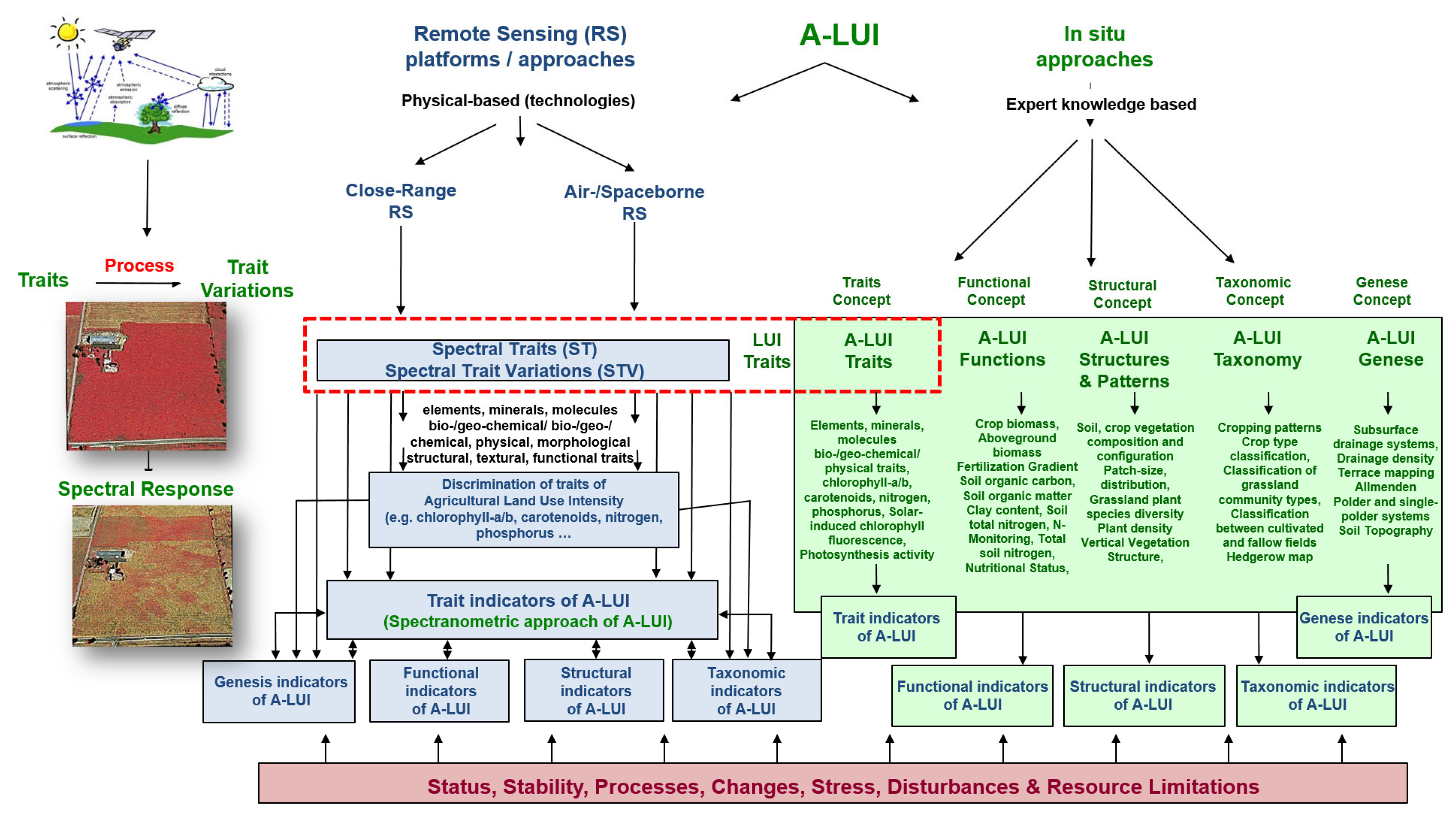
Figure 2.
Different RS platforms; wireless sensor networks (WSN); WSN over lysimeters, Phenotyping laboratories, Global change Experimental Facility (GCEF), Drones, Towers, Balons, airborne-and spaceborne RS platforms withand differnet RS technologies (RGB/photography, multispectral, hyperspectral, thermal, laser, RADAR, acoustic and LiDAR) to monitor indicators of land use intensity on different spatial and temporal scales (modified from Lausch et al. [63]).
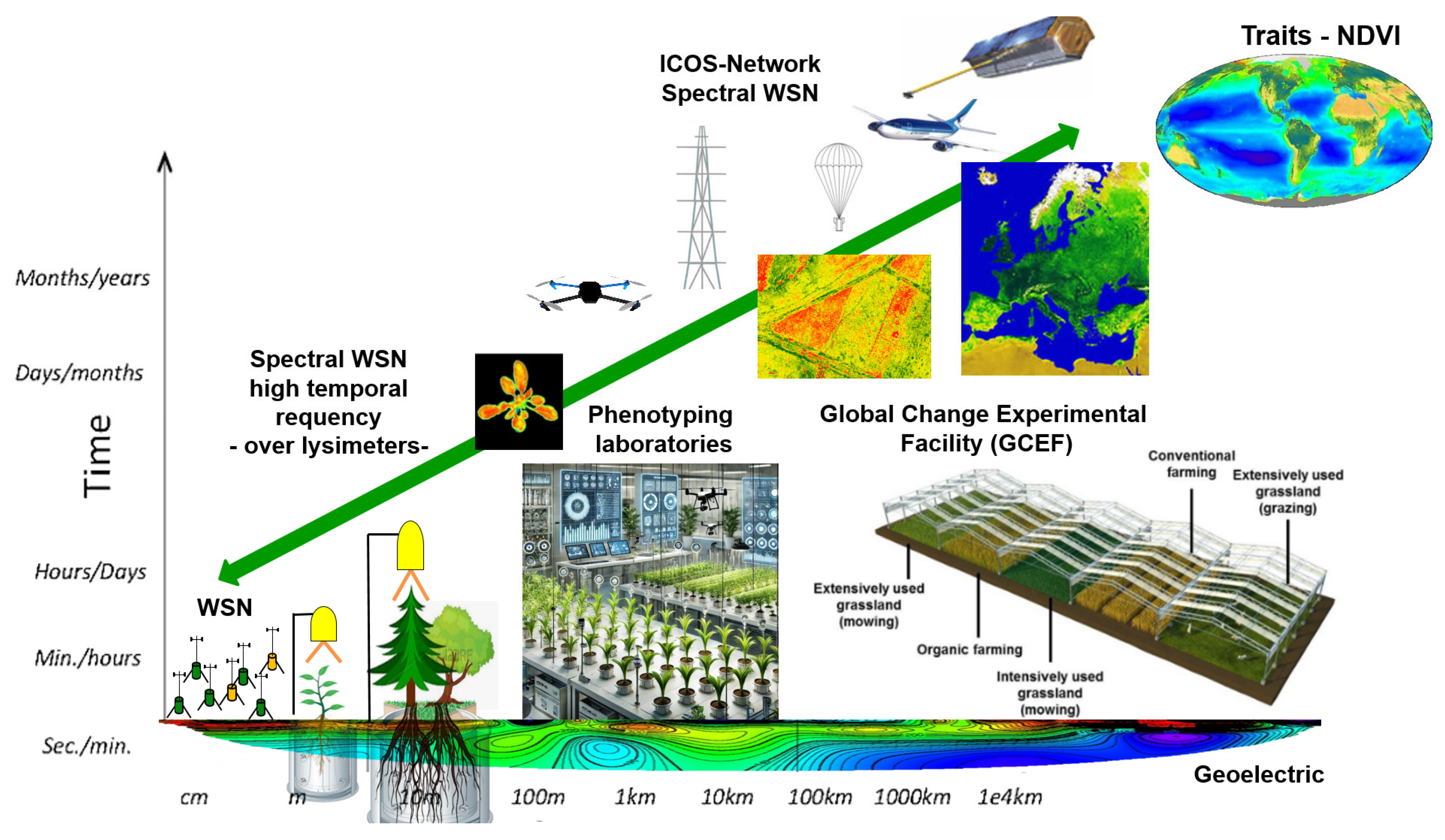
Figure 3.
Problems of spatial resolution of RS data in the detection of crop vegetation, (a) Image of a rapeseed plant at a flight altitude of 1 m with a ground resolution of 0.6 mm per pixel. (b) Image of a rapeseed plant at a flight altitude of 5 m with a ground resolution of 1.5 mm per pixel. (c) Image of a rapeseed plant at a flight altitude of 10 m with a ground resolution of 2.5 mm per pixel. (d) Image of a rapeseed plant at a flight altitude of 20 m with a ground resolution of 5 mm per pixel. (e) Image of a rapeseed plant at a flight altitude of 40 m with a ground resolution of 10 mm per pixel. (f) Image of a rapeseed plant at a flight altitude of 80 m with a ground resolution of 20 mm per pixel (from Grenzdörffer, (Grenzdörffer, G., 2022. Grundlagen der landwirtschaftlichen Fernerkundung https://www.ktbl.de/fileadmin/user_upload/Artikel/Pflanzenbau/Drohnenfernerkundung/Drohnenfernerkundung.pdf.).
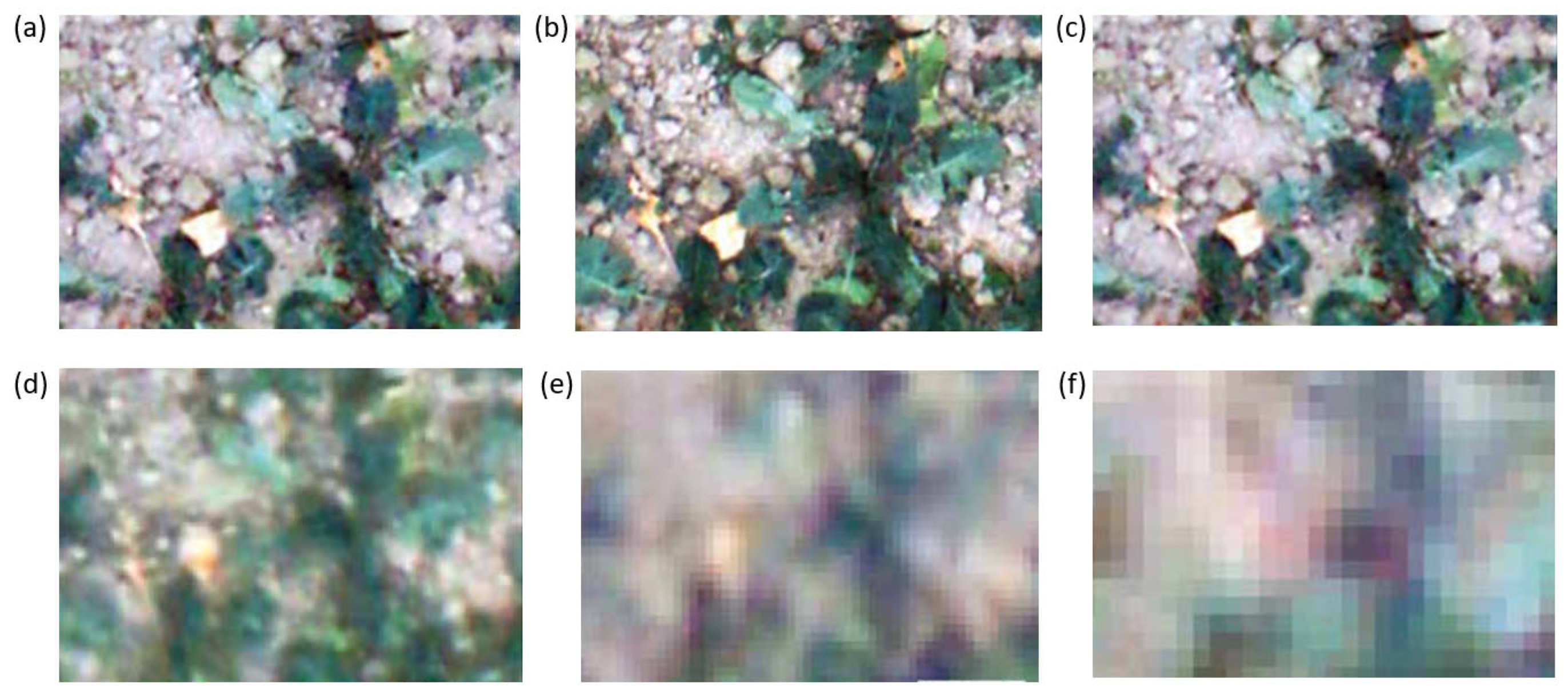
Figure 4.
RS monitoring of the five characteristics of agrariultural LUI (A-LUI), (I) the trait indicators of A-LUI, (II) the genesis indicators of A-LUI, (III) the structural indicators of A-LUI, (IV)) the taxonomic indicators of A-LUI, and (V) the functional indicators of A-LUI. (a) Chlorophyll value, (b) phosphorus value, (c) terrace detection, (d) perimeter boundaries of farmland blocks, (e) shape, size and small-scale nature of the border between Saxony-Anhalt and Lower Saxony, (f) hedgerow map classifications from an aerial photography and (g) TerraSAR-X image, (h) wall-to-wall crop type mapping using the bendchmark 10-day interval composite of Landsat and Sentinel-2 time series, types of grassland management intensity at the Podlaskie study sites, (i) extensive, (j) intensive, (k) disease severity prediction in sugar beet using UAV multispectral data, (l) mean SOC content and (m) C:N ratio maps predicted with Sentinel 1, Sentinel-2 and Landsat-8 data (modified after Lausch et al. [63]).
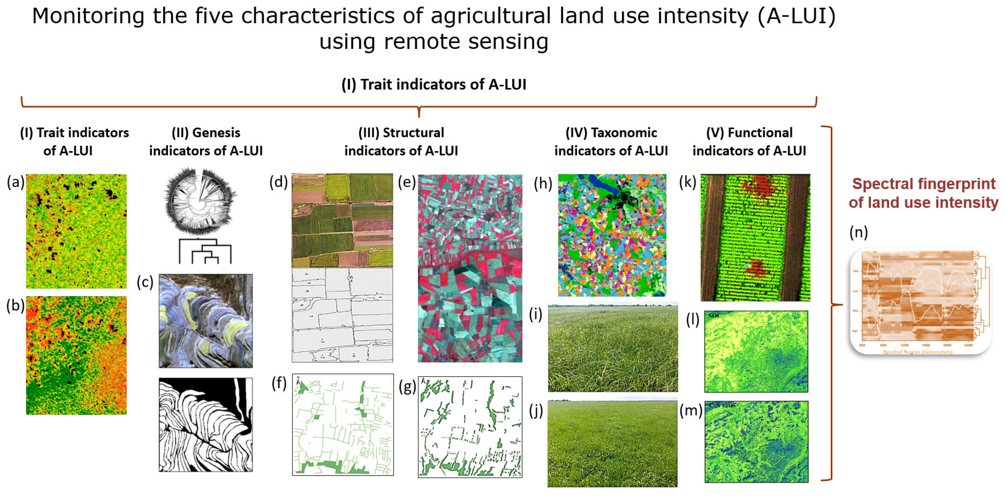
Figure 5.
Mapping spatial nutritional variability of (a) sugarcane (b) foliar chlorophyll, (c) foliar Nitrogen, (d)
phosphorus, (e) potassium concentrations using a MicaSense RedEdge-P camera attached to a drone and LiDAR
data (from Picado and Romero [87]).
Figure 5.
Mapping spatial nutritional variability of (a) sugarcane (b) foliar chlorophyll, (c) foliar Nitrogen, (d)
phosphorus, (e) potassium concentrations using a MicaSense RedEdge-P camera attached to a drone and LiDAR
data (from Picado and Romero [87]).
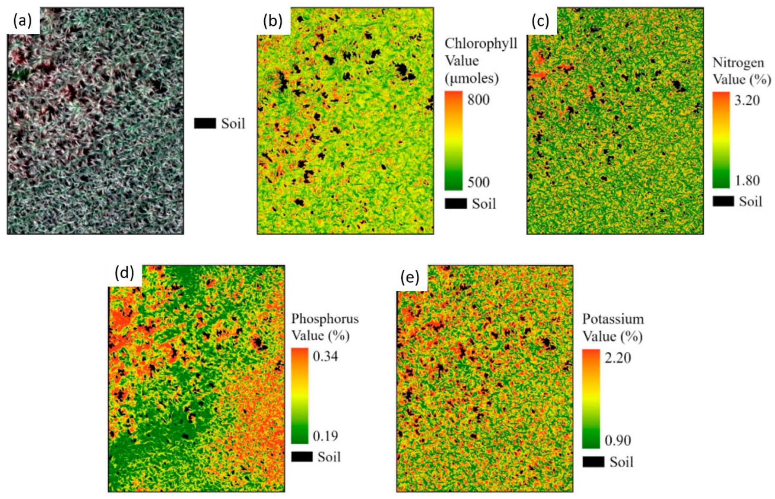
Figure 6.
Spatial distribution of chlorophyll content over the maize field for vegetative stages based on UAV-MS data, (a) early vegetation, (b) mid vegetation, (c) late vegetation, (d) early reproductive, (e) mid reproductive, (f) late reproductive (from Brewer et al. [97]).
Figure 6.
Spatial distribution of chlorophyll content over the maize field for vegetative stages based on UAV-MS data, (a) early vegetation, (b) mid vegetation, (c) late vegetation, (d) early reproductive, (e) mid reproductive, (f) late reproductive (from Brewer et al. [97]).
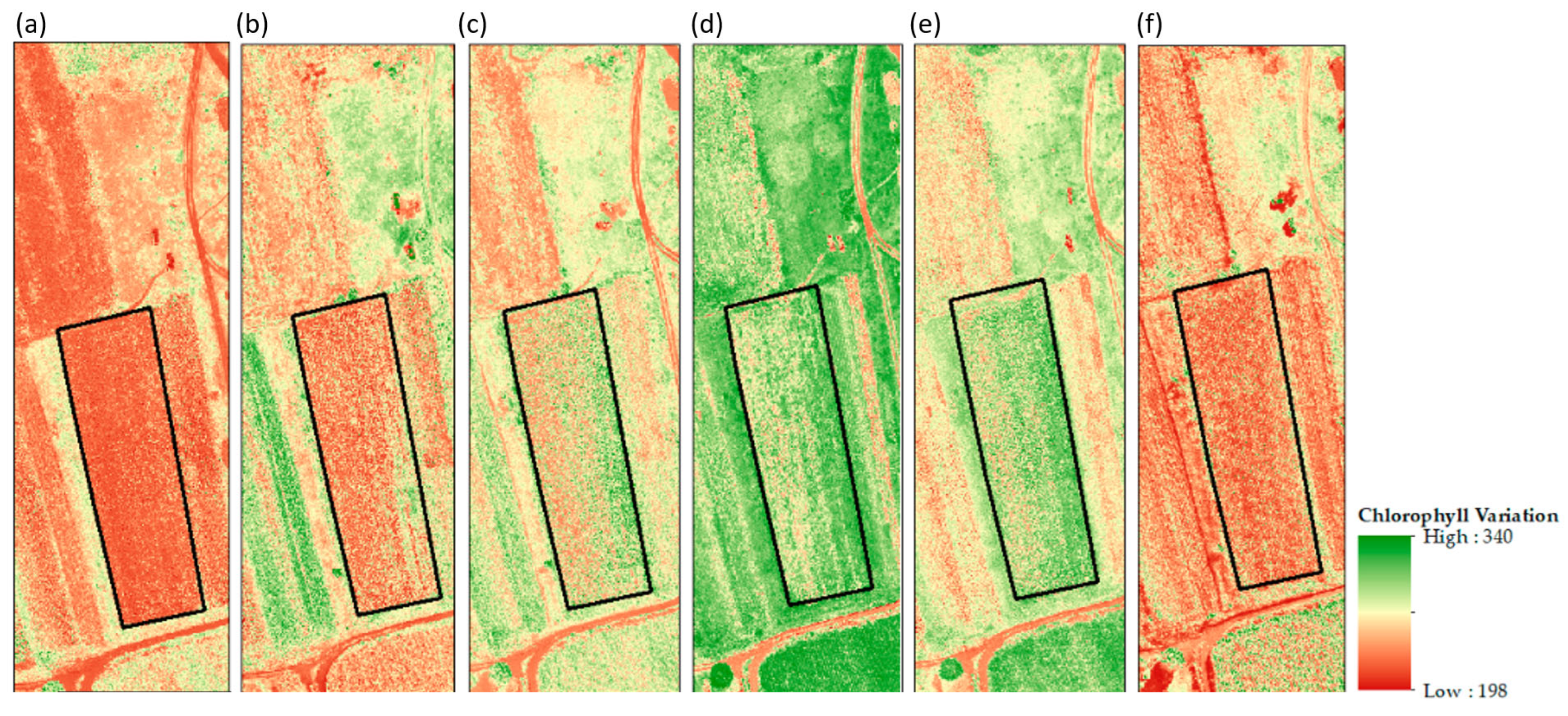
Figure 7.
(a) Reflectance and canopy SIF (b) maps obtained with the HyPlant airborne sensor over an agricultural research site in Klein Altendorf, Germany. Lower SIF is evident in forests (left in lower panel) and higher SIF in dense agricultural fields (middle and right in lower panel). Fluorescence emission reveals information on vegetation status which is not visible in the reflectance domain. For example, the two fields denoted as A and B display almost identical reflectance (b), whereas their fluorescence emission is very different (a) (from Mohammed et al. [72]).
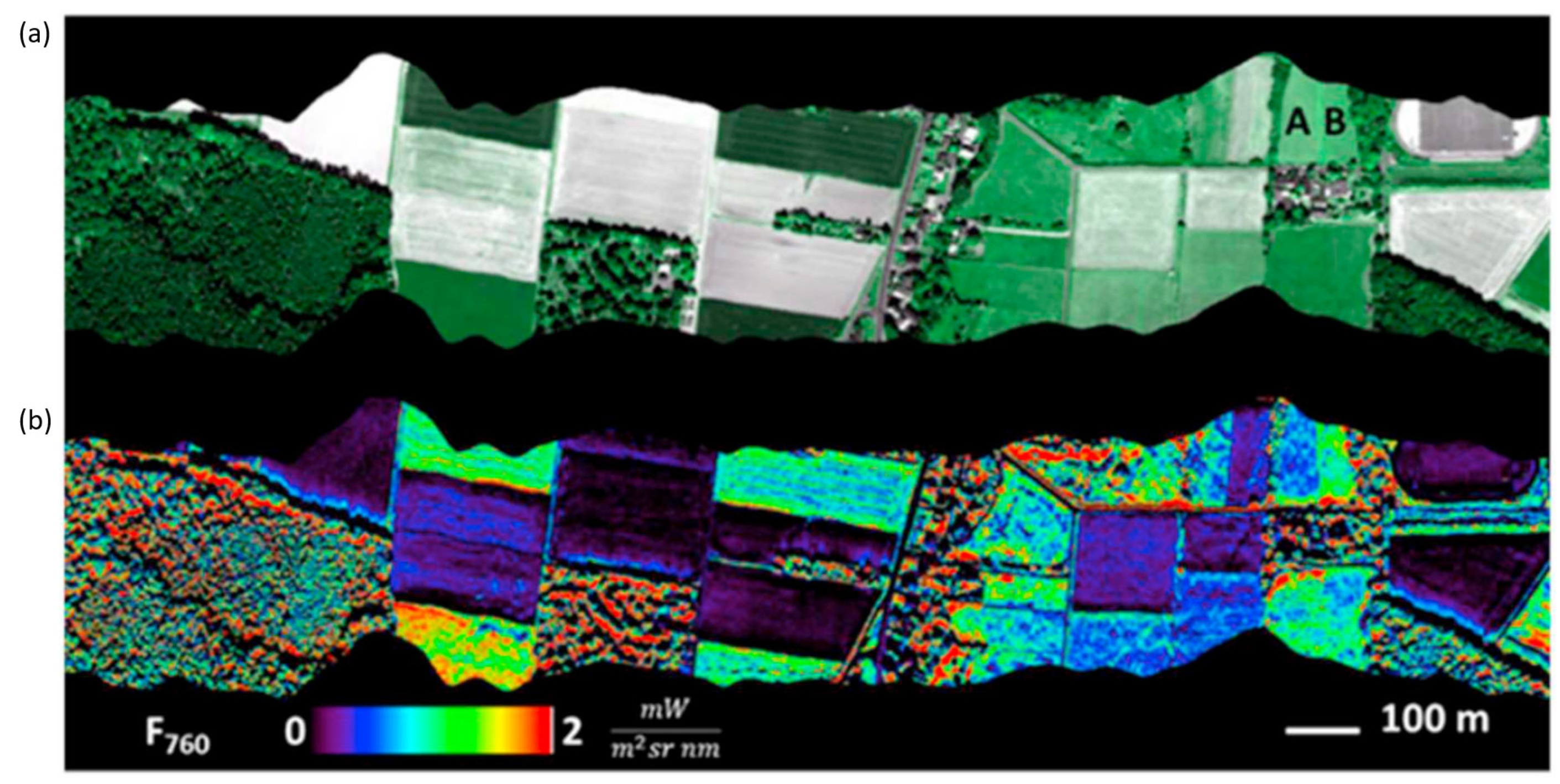
Figure 8.
Estimated leaf N maps for the 2021 pre-harvest season based on models (a) airborne hyperspectral-derived Cab and SIF from tree crowns, and (b) Sentinel-2-derived plant traits Cab, Cw, and Cdm. (from Wang et al., [112]).
Figure 8.
Estimated leaf N maps for the 2021 pre-harvest season based on models (a) airborne hyperspectral-derived Cab and SIF from tree crowns, and (b) Sentinel-2-derived plant traits Cab, Cw, and Cdm. (from Wang et al., [112]).
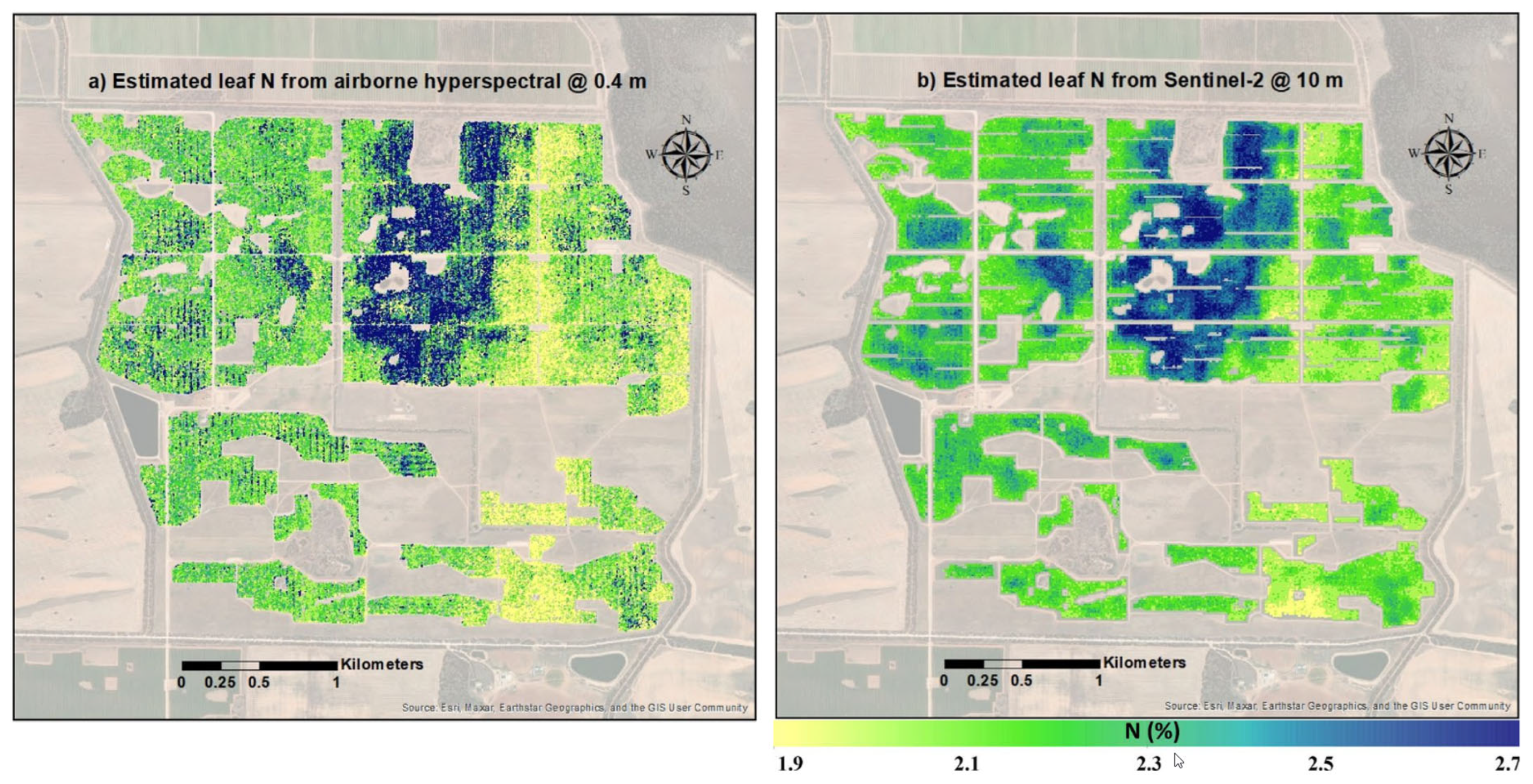
Figure 9.
(a) Location of the study site within the Aak Openings regions in Ohio, USA. (b,c) section of visible image with dull color linear feature interpreted as drainage tile with a parallel network, d) the UAV used to acquire image, (e,f) a section of thermal infrared images of the study site with drainage tile (from Becker et al., [128]).
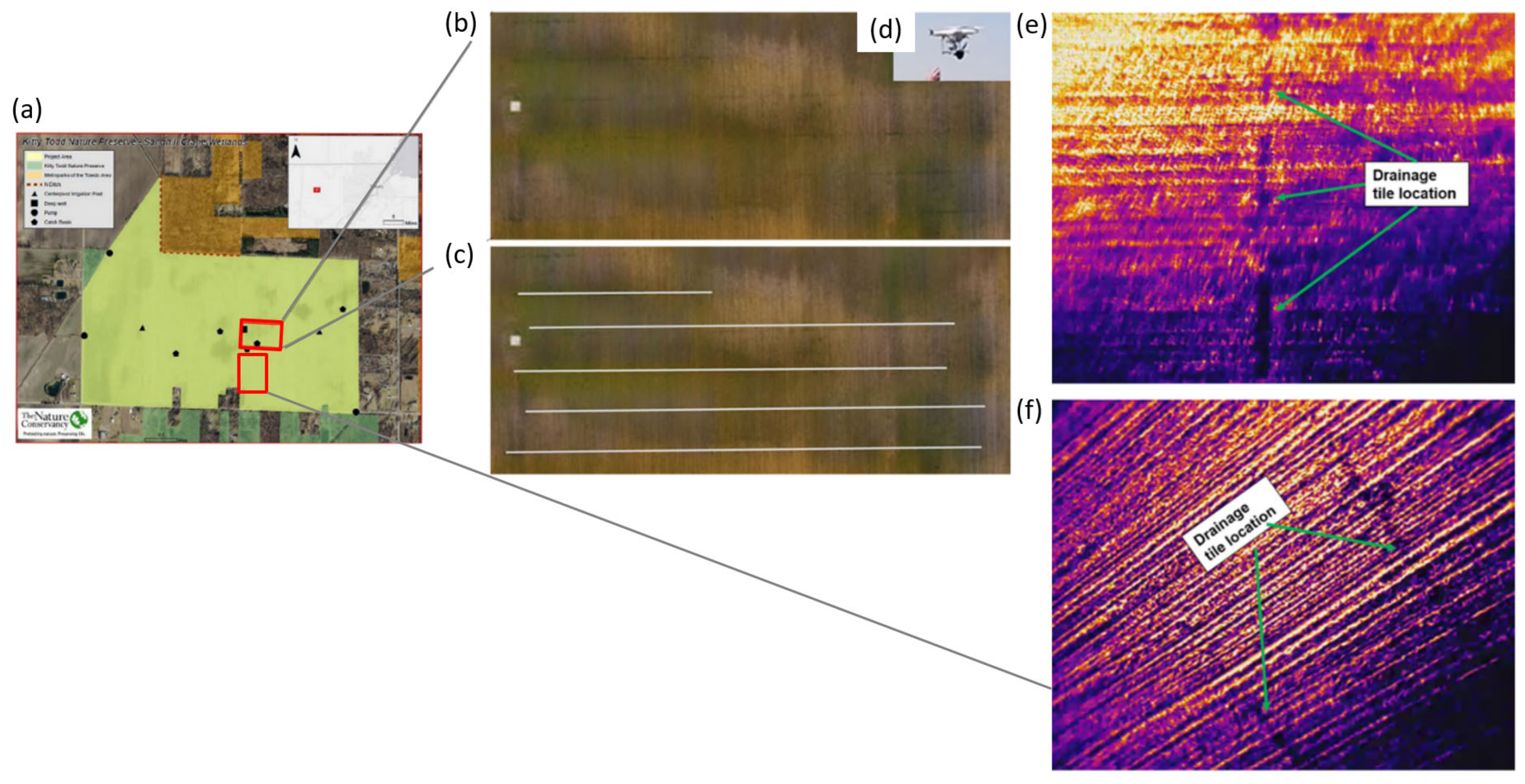
Figure 10.
GF-2 RS Data of fused image and their corresponding labels for detection of terrace. The top row shows the GF-2 RS Dataset of fused images. The bottom row represents the true labels correponding to the GF-2 sample set of fused images (From Yu et al.[131] ).
Figure 10.
GF-2 RS Data of fused image and their corresponding labels for detection of terrace. The top row shows the GF-2 RS Dataset of fused images. The bottom row represents the true labels correponding to the GF-2 sample set of fused images (From Yu et al.[131] ).
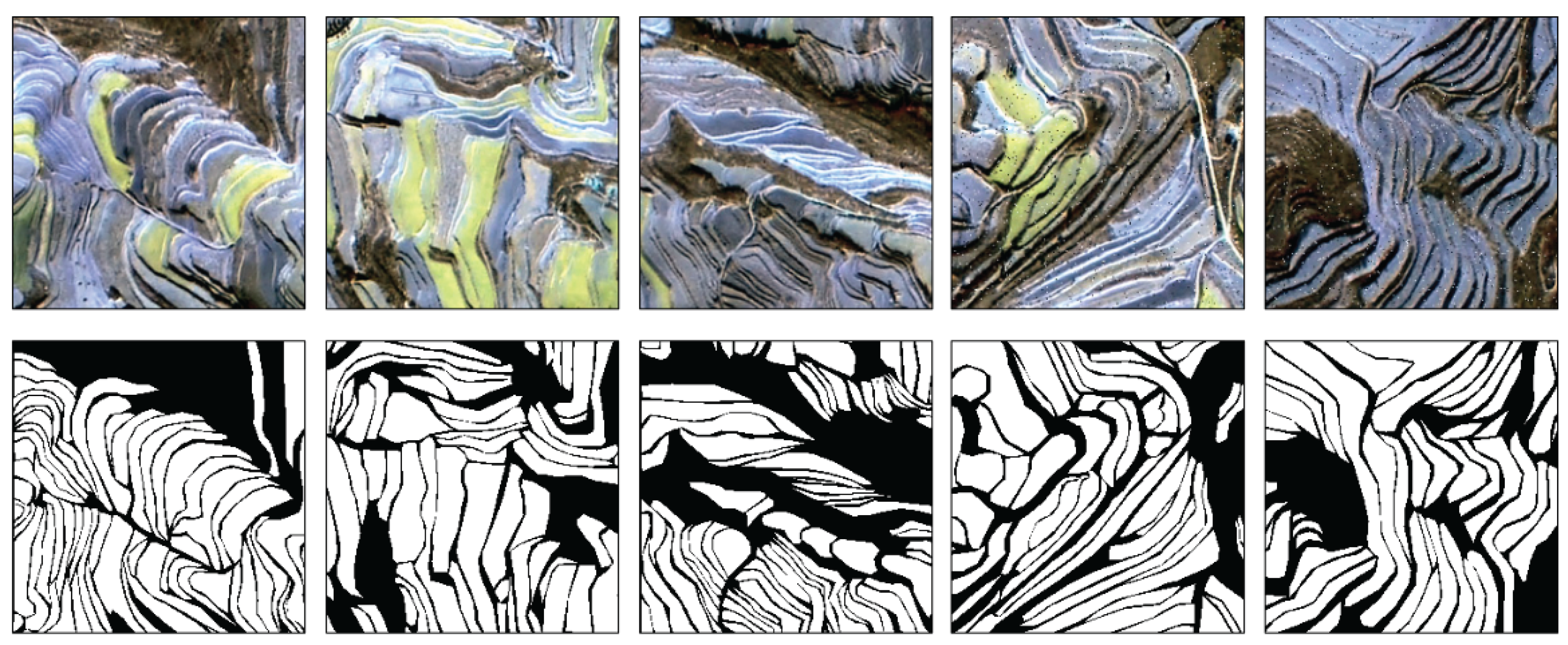
Figure 11.
The deforestation events detected from the time series of photosynthetic vegetation in the Peruvian site. Deforestation is for the period from 2006 to 2016 and it was detected using the mean and standard deviation of RS time series data (Landsat 1990-2016) (from Tarazona et al. [147]).
Figure 11.
The deforestation events detected from the time series of photosynthetic vegetation in the Peruvian site. Deforestation is for the period from 2006 to 2016 and it was detected using the mean and standard deviation of RS time series data (Landsat 1990-2016) (from Tarazona et al. [147]).
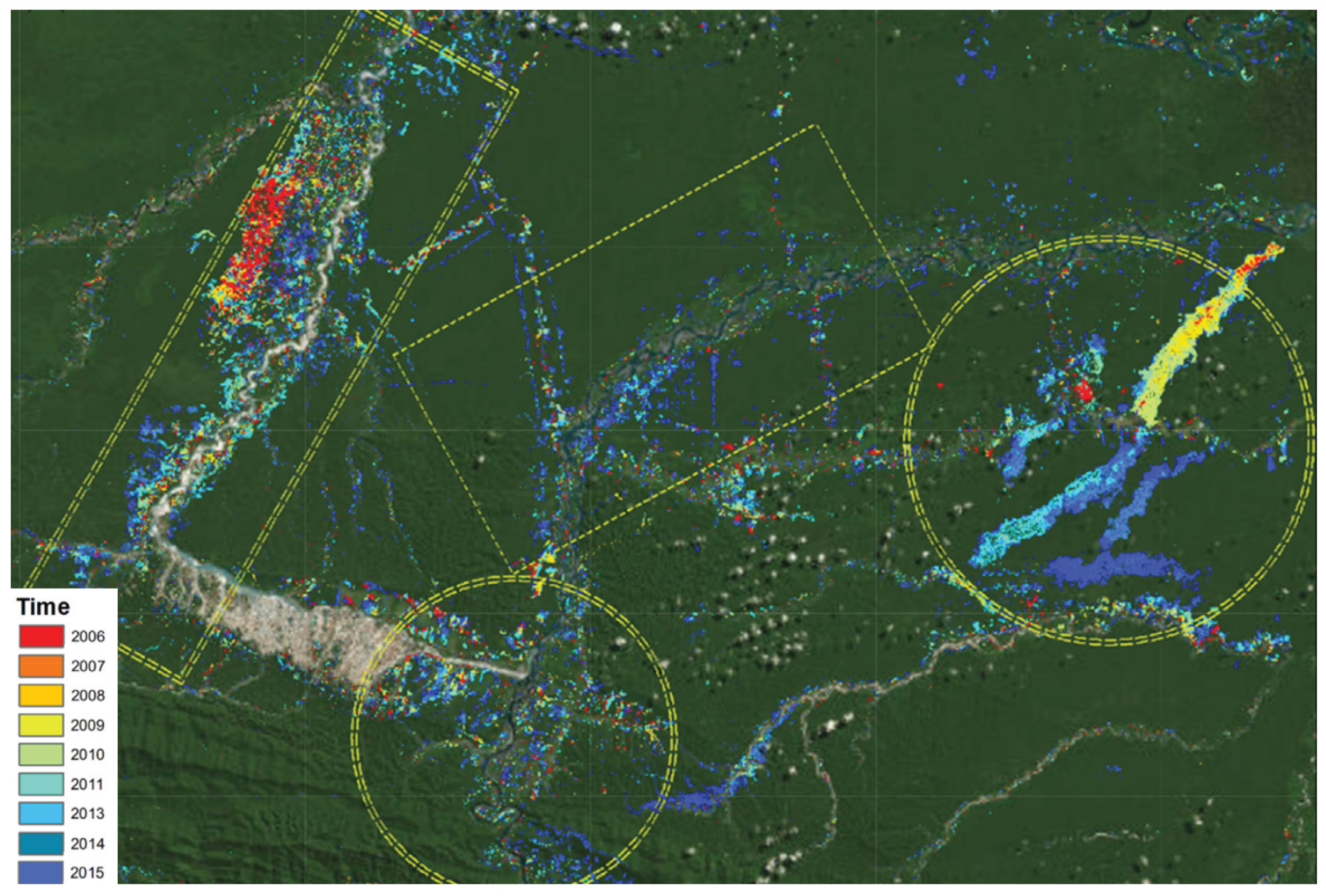
Figure 12.
Different forms of farmland boundaries in RS imagery: (a) threads in farmland imagery, (b) demarcation lines between farmlands, (c) boundary objects between farmlands, (d) perimeter boundaries of farmland blocks, (d) is the the number of the farmland forms of farmland boundaries monitored by RS (from Wang et al. [148]).
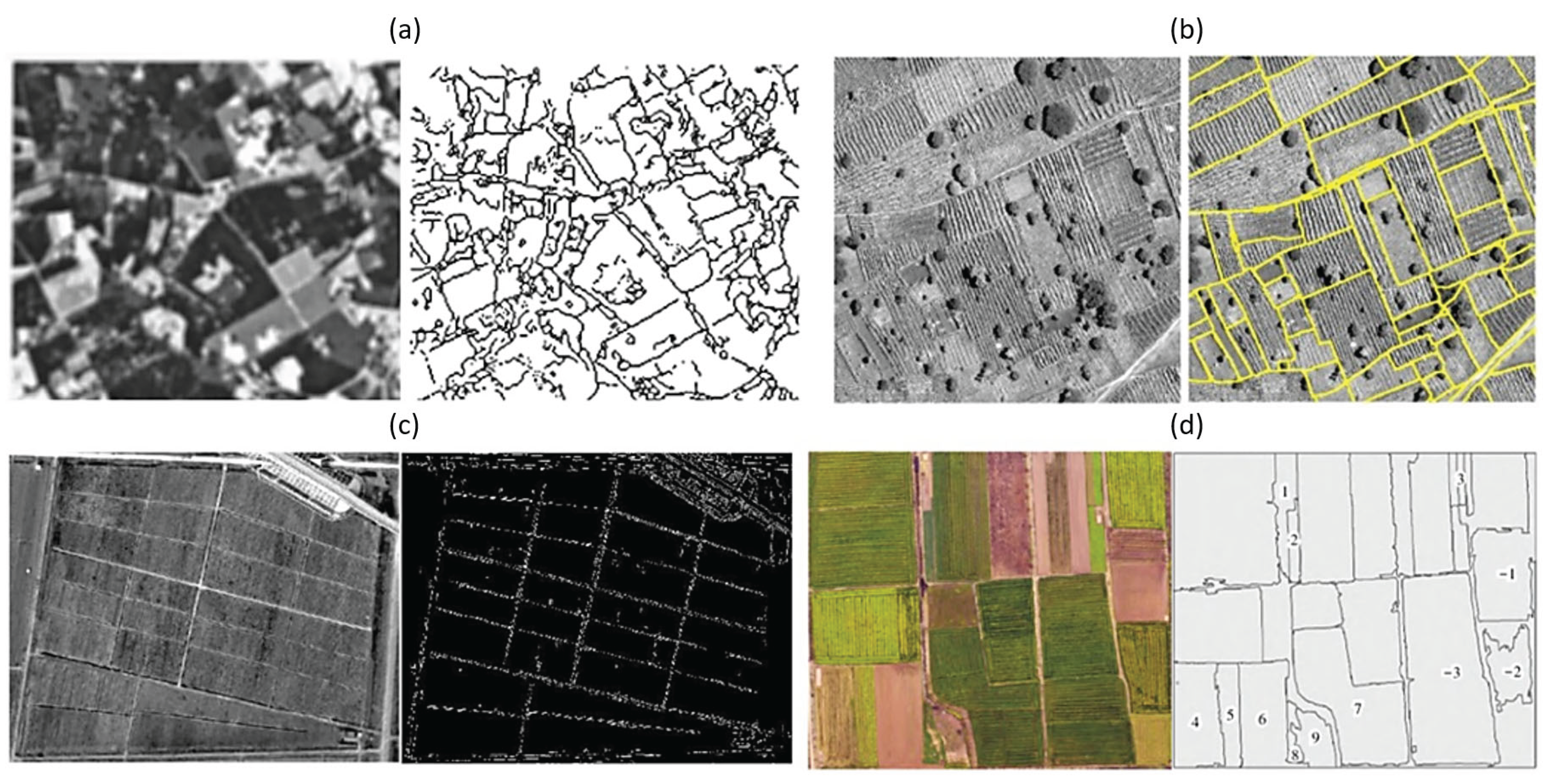
Figure 13.
State border between the former FRG and GDR (different farming practices) after the fall of the Wall is clearly visible due to the shape, size and small-scale nature of the border between Saxony-Anhalt and Lower Saxony north of the Harz Mountains in the 1990s, Germany.
Figure 13.
State border between the former FRG and GDR (different farming practices) after the fall of the Wall is clearly visible due to the shape, size and small-scale nature of the border between Saxony-Anhalt and Lower Saxony north of the Harz Mountains in the 1990s, Germany.
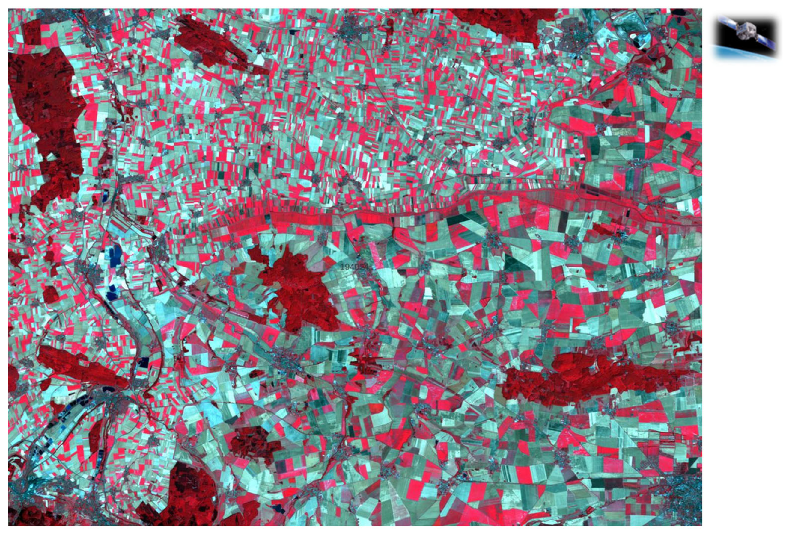
Figure 14.
Normalised termographic reflectivity profile across three fields (corn, wheat and barley) based on RADAR RS data (from Steele-Dunne et al. [162]).
Figure 14.
Normalised termographic reflectivity profile across three fields (corn, wheat and barley) based on RADAR RS data (from Steele-Dunne et al. [162]).
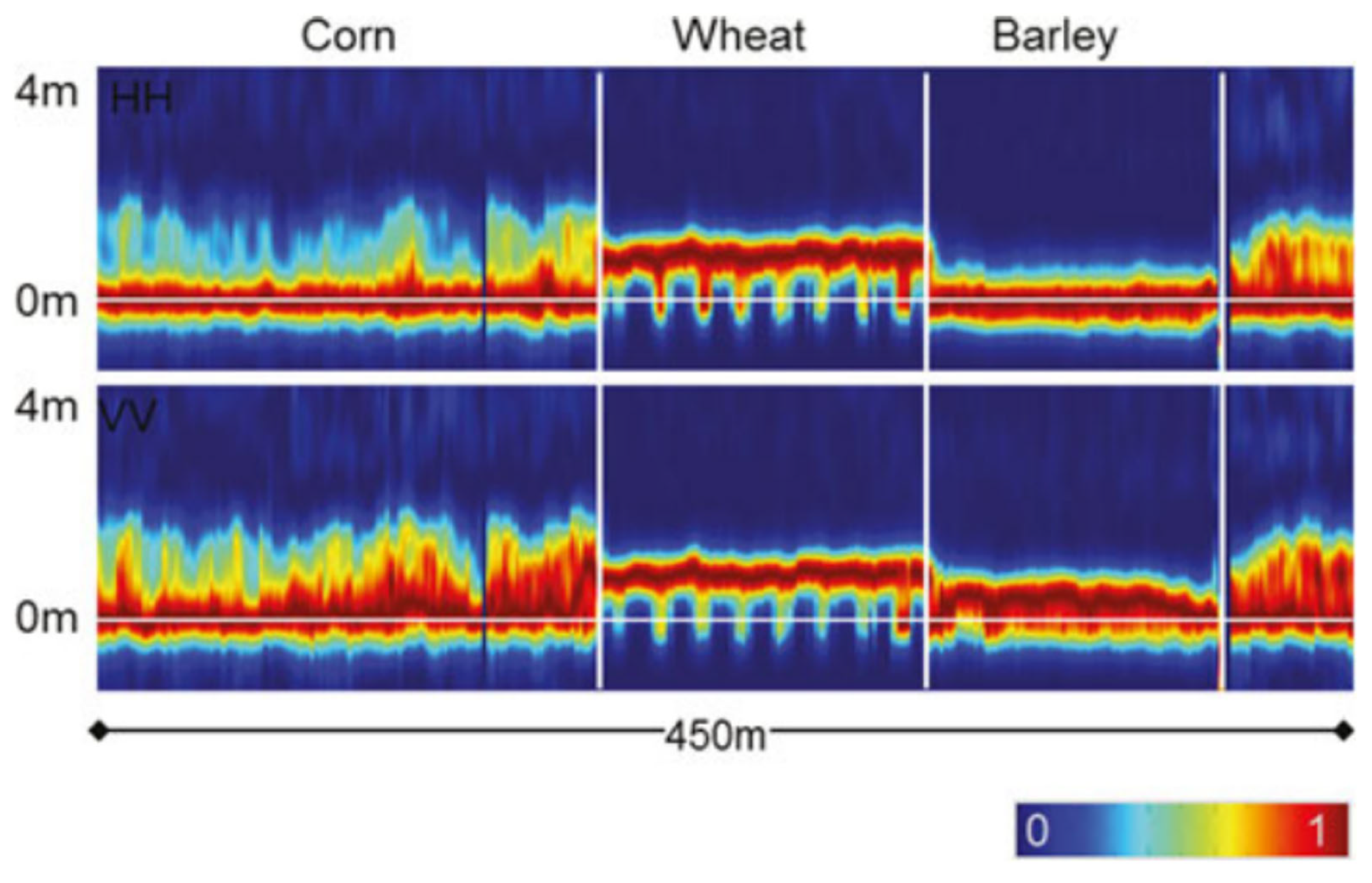
Figure 15.
Field photographs to illustrate the surface roughness conditions in different agricultureal platz on the Kosi Fan. (a) shows the photograph of a stubble field, (b) harrow field, (c) ploughed field, (d) furrow field, (e) surface undulation profile extracted processing the photographs captured for the pin-profile using a digital camera in the field (from Singh et al. [166]).
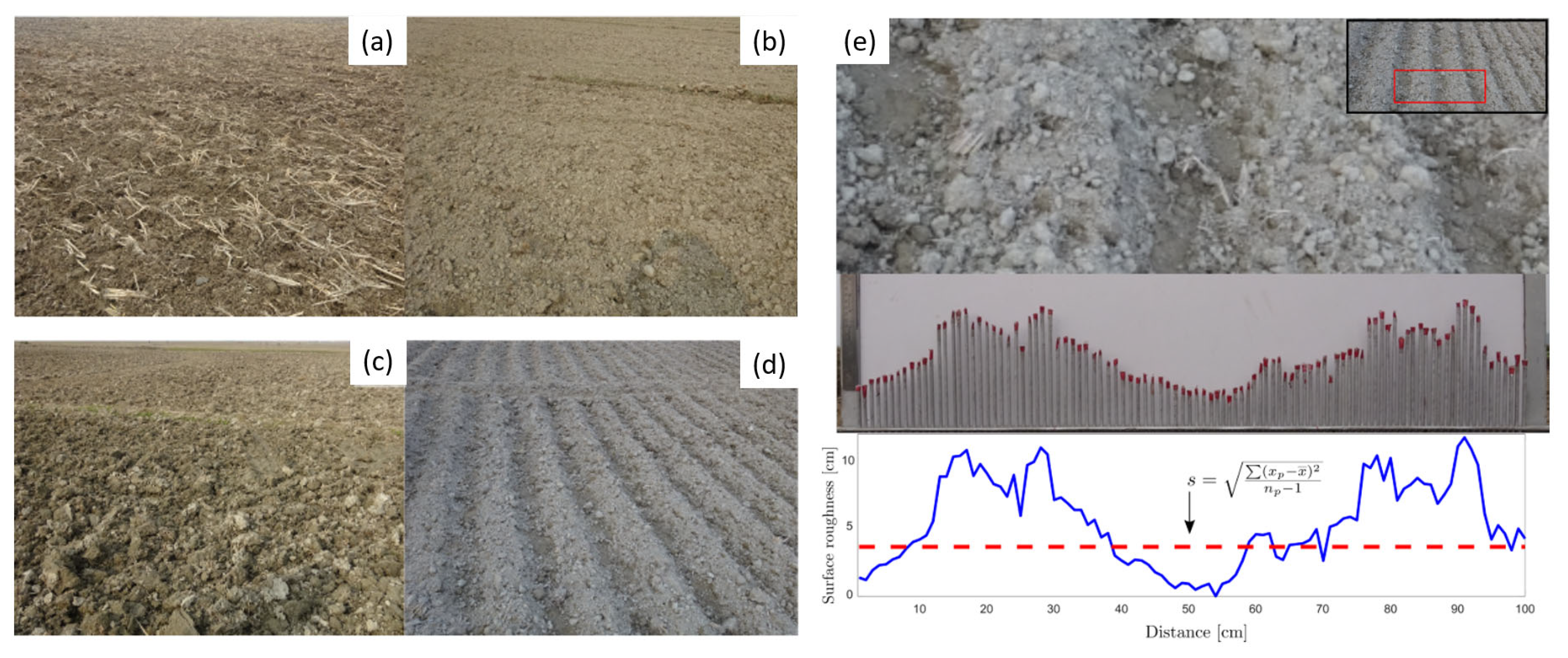
Figure 16.
(a) Image in the top left shows the location of the Kosi megafan in the Himalayan Foreland, (b) spatial distributuion of surface roughness prediction from Sentinel-1, Sentinel-2 and Shuttle RADAR Topographic Mission (SRTM) data. (from Singh et al. [166]).
Figure 16.
(a) Image in the top left shows the location of the Kosi megafan in the Himalayan Foreland, (b) spatial distributuion of surface roughness prediction from Sentinel-1, Sentinel-2 and Shuttle RADAR Topographic Mission (SRTM) data. (from Singh et al. [166]).
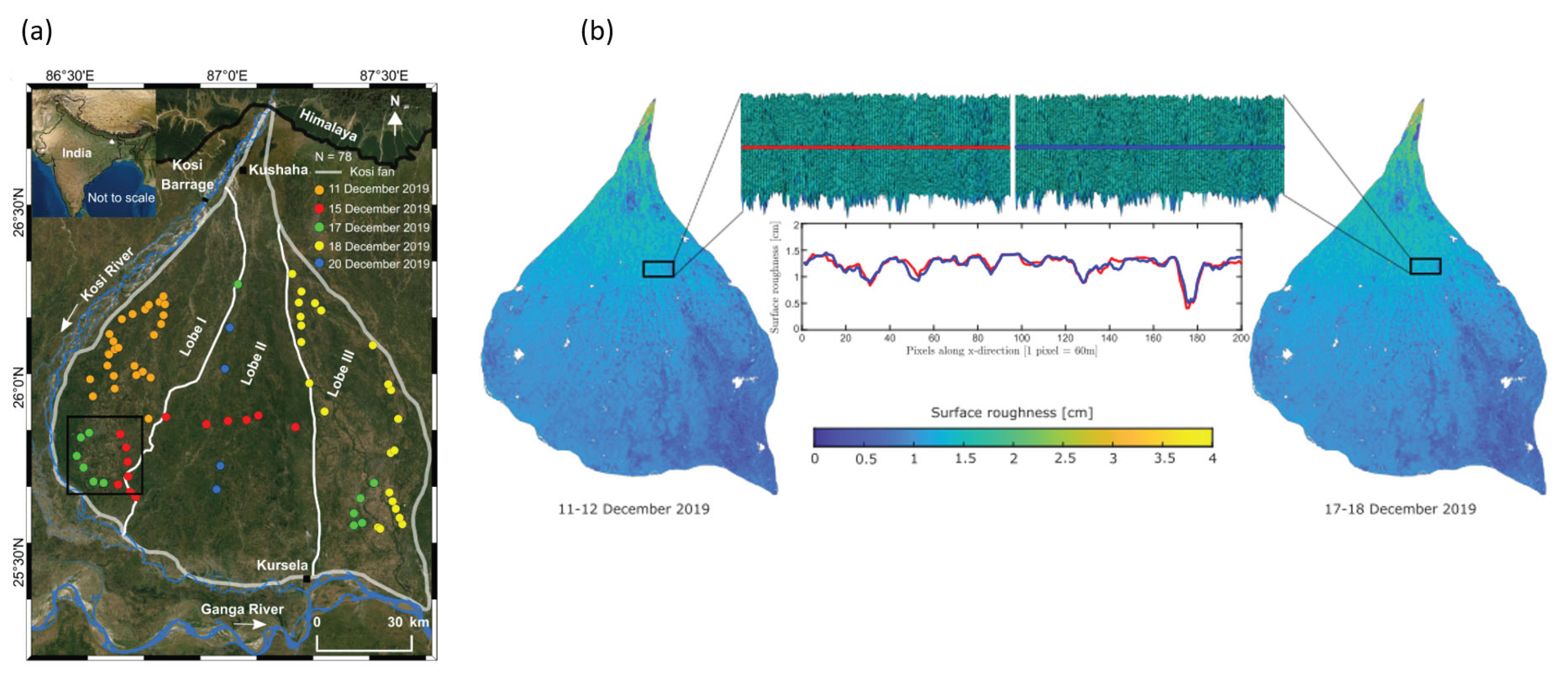
Figure 17.
Results of the wall-to-wall crop type mapping using the bendchmark 10-day interval composite of Landsat and Sentinel-2 time series for Germany (from Griffiths et al. [182]).
Figure 17.
Results of the wall-to-wall crop type mapping using the bendchmark 10-day interval composite of Landsat and Sentinel-2 time series for Germany (from Griffiths et al. [182]).
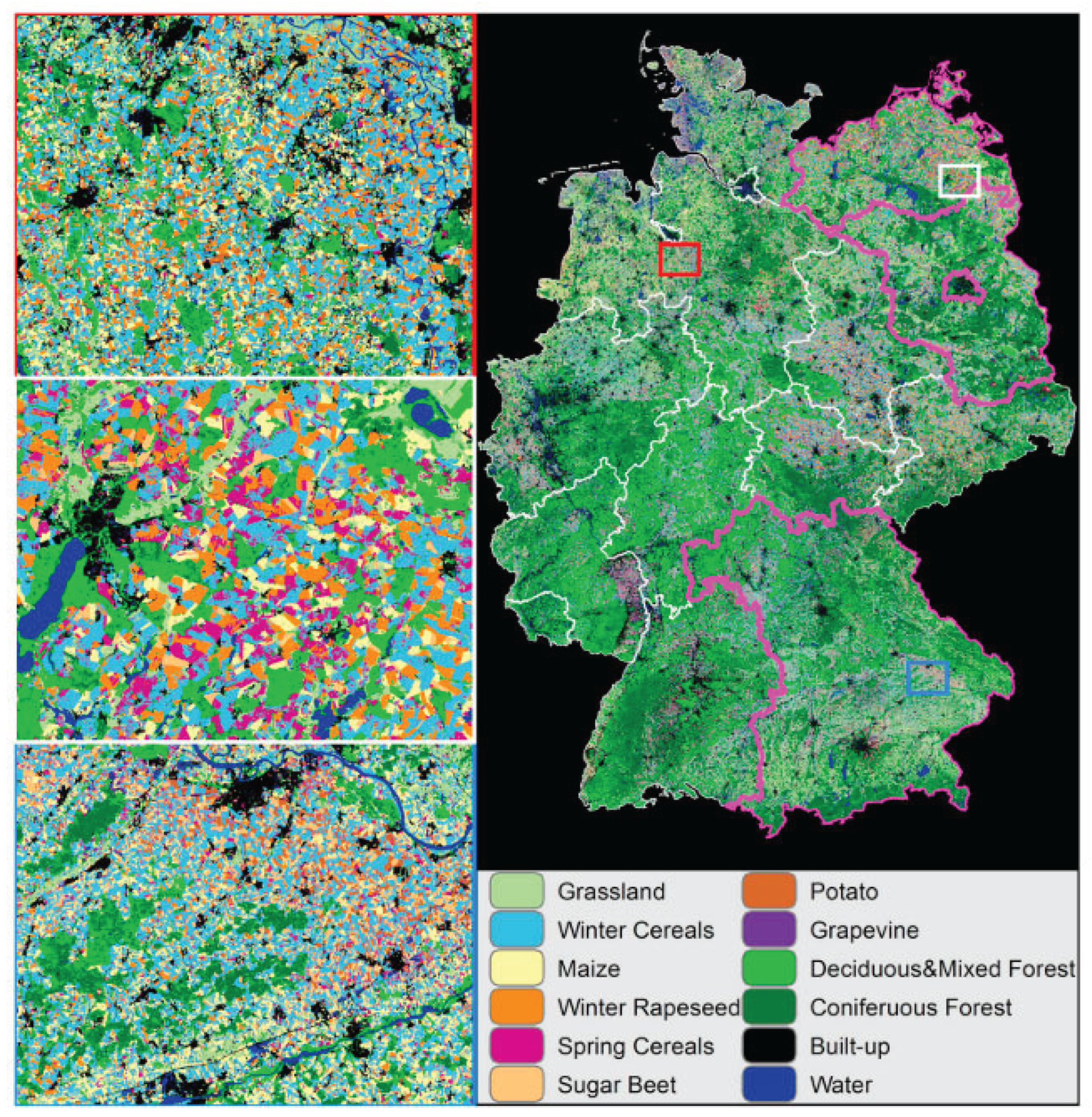
Figure 18.
Types of grassland management intensity at the Podlaskie study sites, (a) extensive, (b) intensive, (c) comparison of spectral curves for intensive and extensive grasslands averaged with the loess algorithm (span = 0.35, confidence interval = 0.95) based on Sentinel-2, (from Bartold et al. [187]).
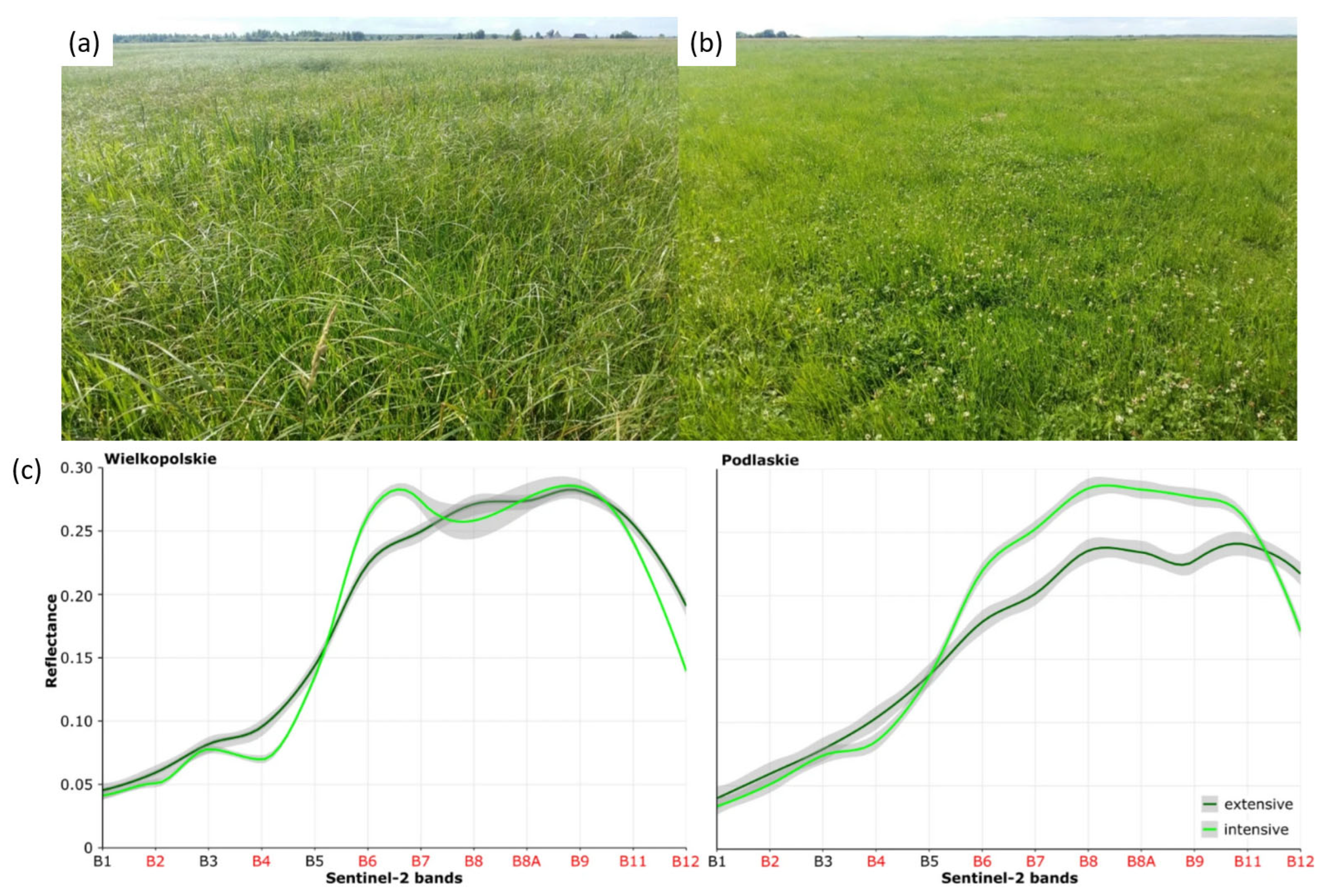
Figure 19.
Difference map of Abovground Biomass (AGB) estimaates of 18. August 2017 and 26. August 2017 derived from PlanetScope (PS) optical, Sentinel-1 Synthetic Aperture RADAR (SAR), and hybrid (optical plus SAR) datasets. Reddish tones indicate AG increase and blue tones indicate AGB decrease. White areas indicate low AGB variation (from Breunig et al. [192]).
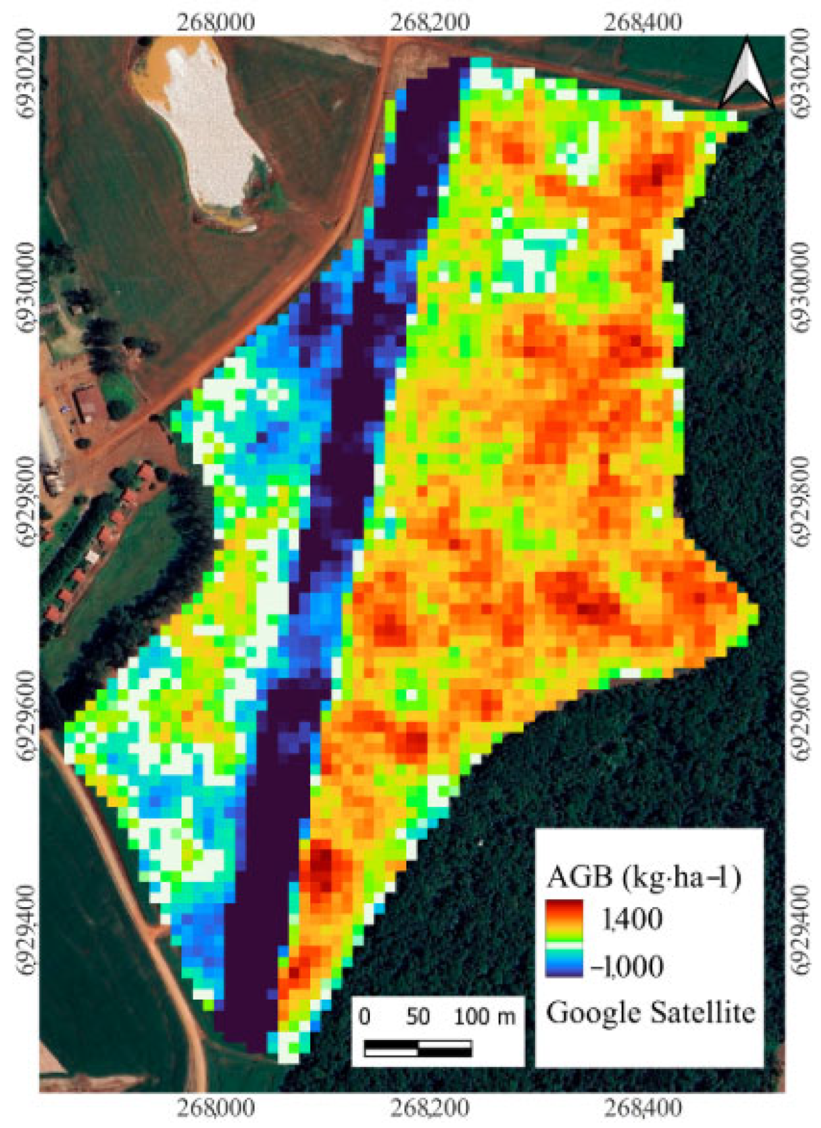
Figure 20.
Exemplary application of SugarViT (Vision Transformer based model for disease severity) for disease severity prediction in sugar beet using UAV multispectral data. Each prediction is completely independent of its surrounding predictions. The model shows a highly consistent prediction behavior (from Günder et al. [202]).
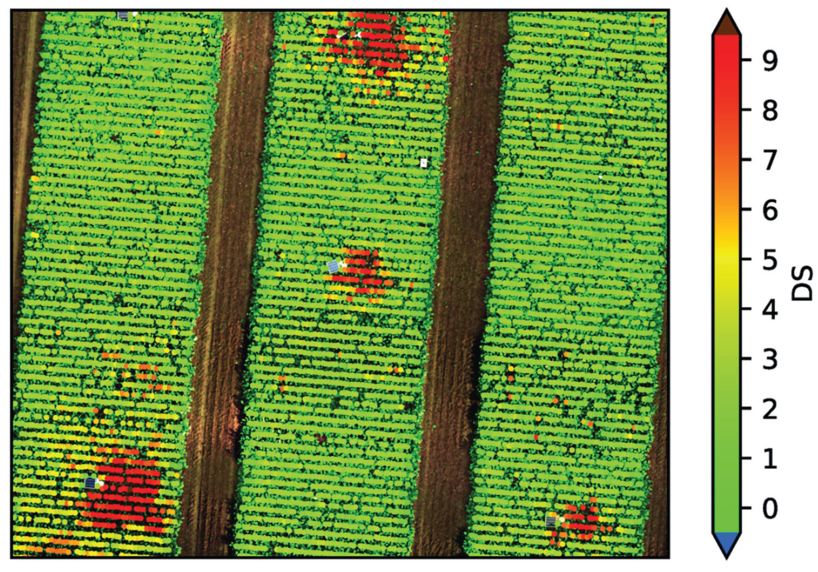
Figure 21.
Mean SOC content and C:N ratio maps predicted by 100 runs of BRT in Model V at a resolution of 100 m and their corresponding standard deviation maps (Model V: all available predictors, Sentinel 1-predictors, Sentinel-2 predictors, Landsat-8 predictors, Climate-predictors, Topography-predictors) (from Zhou et al. [222]).
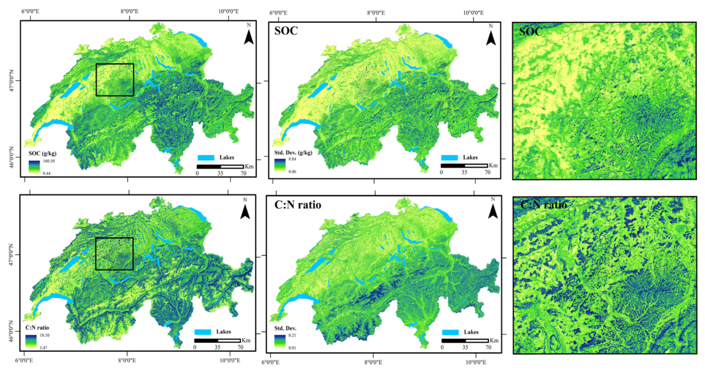
Figure 22.
Semantic data integration for assessing agricultural land use intensity. Integration of diverse data sources (satelite data, soil data, agricultural statistics, research databases, socioeconomic information, model data.
Figure 22.
Semantic data integration for assessing agricultural land use intensity. Integration of diverse data sources (satelite data, soil data, agricultural statistics, research databases, socioeconomic information, model data.
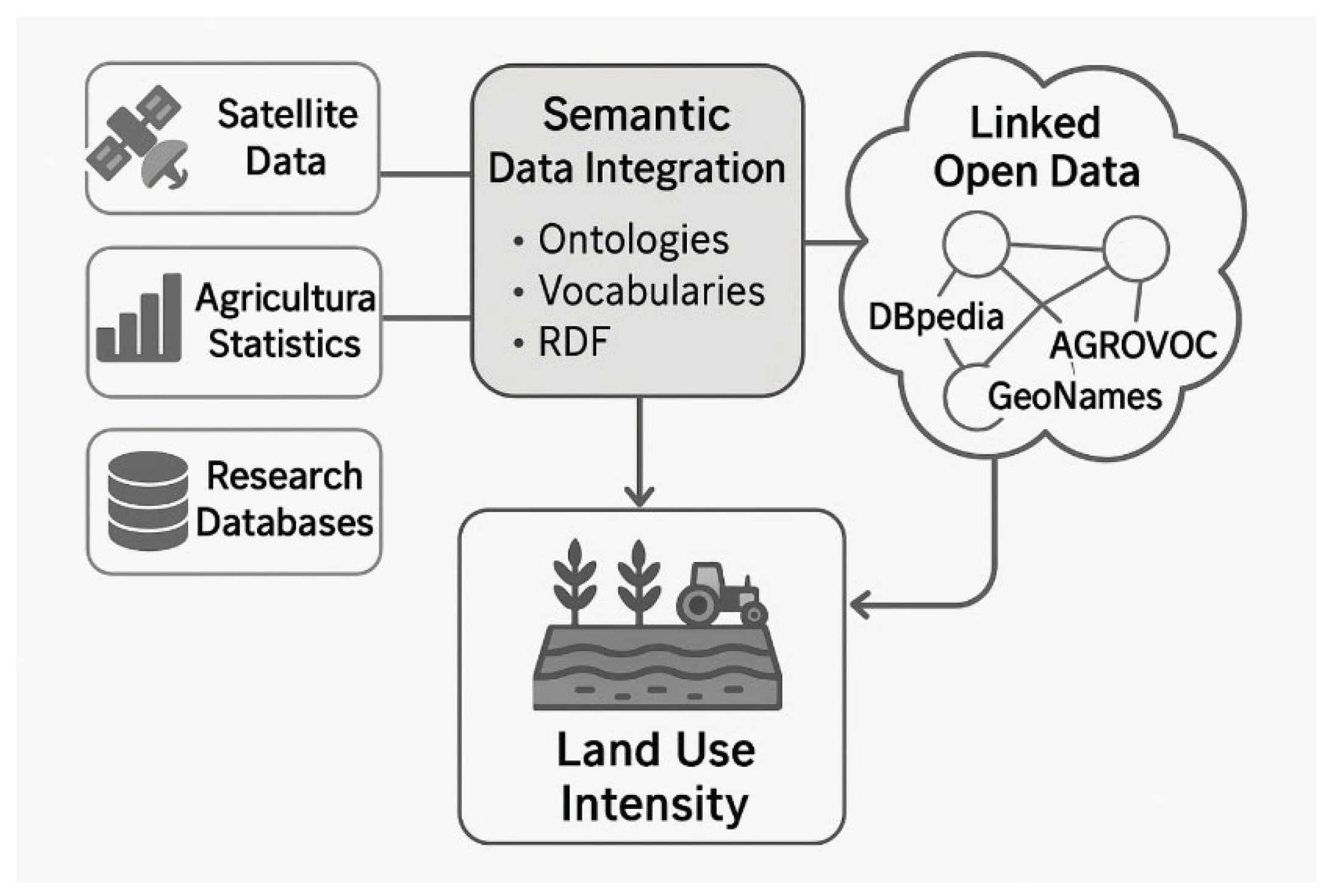
Disclaimer/Publisher’s Note: The statements, opinions and data contained in all publications are solely those of the individual author(s) and contributor(s) and not of MDPI and/or the editor(s). MDPI and/or the editor(s) disclaim responsibility for any injury to people or property resulting from any ideas, methods, instructions or products referred to in the content. |
© 2025 by the authors. Licensee MDPI, Basel, Switzerland. This article is an open access article distributed under the terms and conditions of the Creative Commons Attribution (CC BY) license (http://creativecommons.org/licenses/by/4.0/).
Copyright: This open access article is published under a Creative Commons CC BY 4.0 license, which permit the free download, distribution, and reuse, provided that the author and preprint are cited in any reuse.


